KEK-TH-1960
Gravitino thermal production revisited and a new cosmological scenario of gauge mediation
Hiraku Fukushima1,2 and Ryuichiro Kitano1,3
1KEK Theory Center, Tsukuba, Japan
2Department of Physics, Tohoku University, Sendai, Japan
3The Graduate University for Advanced Studies (Sokendai), Tsukuba, Japan
Abstract
We present a new scenario of gravitino dark matter which is compatible with the thermal leptogenesis. We confirm by an explicit calculation in supergravity that the relic abundance of thermally produced gravitino becomes insensitive to the reheating temperature once the temperature of the Universe exceeds the mass scale of the messenger fields. In such a situation, the correct baryon to dark matter ratio can be obtained by thermal leptogenesis when the reheating temperature after inflation is high enough. We demonstrate in a concrete model of gauge mediation that the correct abundance of gravitino and baryon asymmetry can be reproduced by considering the late-time entropy production from the decay of the SUSY-breaking pseudo-moduli field. The scenario is realized when the gravitino mass is , and the messenger mass scale is .
1 Introduction
The existence of dark matter (DM) is the clearest hint to physics beyond the Standard Model (SM). Among various candidates to explain the unknown component of the Universe, the hypothesis of gravitino dark matter is very attractive as the gravitino always exists in supersymmetric (SUSY) theories and is often the lightest superparticle (LSP) since its mass is suppressed by the Planck scale. The gauge mediated SUSY breaking (GMSB) scenario [1, 2] is an explicit realization of the gravitino LSP while the superpartners of the SM particles can be much heavier due to the SM gauge interactions.
In the GMSB models, gravitinos are produced in the early Universe from the thermal bath of the particles in the minimal supersymmetric standard model (MSSM). The production process is more effective at high temperatures, and thus the relic abundance is proportional to the reheating temperature after inflation [4, 5, 6, 7, 8, 9, 10, 11, 12, 13], . This gives an upper bound on so as not for the gravitino abundance to exceed the observed DM abundance, . The upper bound is for and it becomes more severe for a lighter gravitino. It is, therefore, difficult to realize the gravitino DM compatible with the thermal leptogenesis [14], where the maximal baryon asymmetry is also proportional to . In order to explain the baron asymmetry of the Universe, we need [15, 16, 17, 18]. The ratio is predicted to be too large compared to the observed one, i.e., . The late-time entropy production do not help this situation since both the baryon and DM are diluted while fixing the ratio, .
The production rate of gravitino has been calculated in the literatures by using the supergravity Lagrangian, which should be correct at low energy. However, it has been argued in Ref. [20], those estimates should be modified in GMSB models for a temperature higher than the messenger scale . The authors of Ref. [20] evaluated the gravitino production rate using the Lagrangian of global SUSY, and found that for temperature , the rate is suppressed by compared to the supergravity calculation. If this is the case, the gravitino relic abundance becomes insensitive to for . The calculations in global SUSY should match the supergravity ones for energies higher than the gravitino mass at the leading order in the expansion.
Although the statement in Ref. [20] is clear in terms of global SUSY, it seems somewhat obscure in the supergravity description. In the global SUSY case, the MSSM fields couple to the goldstino (the longitudinal component of the gravitino) only though the loops of the messenger fields. The production rate is, therefore, significantly modified when the energy goes beyond the mass of the messenger fields. On the other hand, in the supergravity Lagrangian, there are contact derivative interactions between the gravitino and the supercurrent made of the MSSM fields, which lead a growth of the amplitude as energy increases. Therefore, in this description, there is no apparent reason for the gravitino production to be suppressed above the messenger scale [21, 22].
In this paper, in order to offer a comprehensive view about the gravitino thermal production, we explicitly calculate a gravitino production process both with a global SUSY Lagrangian and a supergravity Lagrangian, independently. We confirm the suppression of the gravitino production rate both in global SUSY and supergravity for even though there is a contact interaction term in the supergravity Lagrangian. It is found that the loop diagrams involving messenger fields in the supergravity calculation cancel the tree-level amplitude at a high energy region. The result agrees with the intuition from the goldstino equivalence. The results indicate that the relic abundance of the gravitino is proportional to the messenger scale, rather than for . Therefore, in this occasion, there is no reason to abandon thermal leptogenesis. Given that the gravitino abundance does not depend on , the ratio can be fixed to the observed value, , with a suitable .
Although the observed DM-baryon ratio can be explained by the thermal leptogenesis, the scenario requires a late-time entropy production by some mechanism, because the produced amount of gravitino is still larger than the observation, , in order to explain the ratio. Interestingly, we already have a source of the entropy production in GMSB models; there is a pseudo-moduli field in generic low-energy SUSY breaking models, which can supply a large amount of entropy by its decay. We demonstrate the scenario in a simple model of gauge mediation and confirm that the scenario indeed works as the mechanism to produce the right amount of the gravitino DM.
The sketch of the scenario is as follows; the reheating of the Universe occurs at a high so that the gravitino abundance is independent of . With an appropriate reheating temperature, the ratio of energy densities can be fixed at the observed value, , after the reheating process. Later, the SUSY breaking pseudo-moduli starts coherent oscillation about the minimum of the potential, and the oscillation energy eventually dominates the Universe. A sizable amount of entropy is released by the subsequent decay, and the pre-existing gravitinos and baryons are diluted by a same amount to realize the observed values.
Throughout our analysis, the SUSY scale is assumed to be to realize [3] within the MSSM. Although it sounds difficult to confirm the scenario by the LHC experiments, the framework we use predicts a relatively small -term and thus there is a light higgsino with . We explain this point in appendix B. Such a light higgsino may be within the reach of future experiments such as at an International Linear Collider (ILC). Since the life-time of higgsino can be as long as sec, we check the constraints from the Big-Bang nucleosynthesis (BBN) and find that the light higgsino is cosmologically safe if the gravitino mass is less than .
2 Gravitino thermal production in GMSB revisited
The gravitino production rate has been calculated by using the supergravity Lagrangian [4, 5, 6, 7, 8, 9, 10, 11, 12, 13], which leads the result that the abundance is proportional to . In GMSB models, the production is dominated by that of the longitudinal mode which can be evaluated by identifying the longitudinal mode as the goldstino in the global SUSY Lagrangian. Moreover, in GMSB models, one can use a framework of a linearly realized SUSY breaking model with a singlet superfield , whose -component VEV breaks the SUSY.
An explicit calculation of the goldstino production shows that the goldstino relic abundance is not necessarily proportional to [20], which contradicts with the estimation in supergravity. We examine this apparent contradiction by calculating the scattering amplitudes of goldstino/gravitino production process both with a global SUSY Lagrangian and a supergravity Lagrangian. We confirm that the supergravity result should be modified at high energy.
2.1 Gravitino thermal production in GMSB
Calculation in supergravity Lagrangian
Here we briefly review why the gravitino relic abundance is determined by the reheating temperature . Gravitinos are produced from the scattering process of the MSSM fields and the amplitudes are calculated by using the supergravity Lagrangian,
| (1) |
where the gravitino field is denoted by . The gravitino has the tree-level interactions with all the chiral multiplets () or gauge multiplets () in the MSSM and the form of interactions is uniquely fixed by local SUSY.
For the gravitino production, there are ten two-body processes involving left-handed quarks (), squarks (), gauginos () and the gauge bosons (), which are called processes A to J in the literatures [4, 5, 6, 8, 9]. In the literatures the QCD processes are discussed in detail because they are the dominant processes. Here we focus on a particular process (called process I in the literatures) for simplicity. The tree-level diagrams are shown in Fig. 1.


The scattering amplitude is calculated by the supergravity Lagrangian in Eq. (1). Among the polarized amplitudes, the following turns out to have the highest power in the center-of-mass energy, , and thus dominates at high energies,
| (2) |
where arrows in the parenthesis represent the spins of the electron, the positron, the gaugino and the gravitino, respectively. The angle is the production angle in the center-of-mass frame. The gauge coupling of QED is denoted by . Although each of -, - and -channel diagrams has an energy dependence of , they are canceled out when combined, remaining the energy dependence of . The above contribution is from the longitudinal component of the gravitino whose wave function is approximately proportional to with the gravitino mass.
In order to estimate the relic abundance of the gravitino, we should calculate the reaction rate which is proportional to the square of the amplitude,
| (3) |
where the temperature dependence is determined by dimensional analysis. The key is the cubic dependence on . If the reaction rate depends on the temperature with a higher power than the Hubble parameter , the resultant gravitino abundance is fixed at high temperature, . In contrast, if the power is lower than , the yield is fixed by the lowest temperature. If the process is effective and Eq. (3) is valid for an arbitrary temperature, the gravitino abundance is determined by .
Goldstino analysis
In GMSB models, effects of SUSY breaking are transmitted to the MSSM sector through the messenger loop diagrams. A superpotential of the following form is usually assumed,
| (4) |
SUSY is broken by the -component of the singlet superfield . and represent the messenger superfields which have SM gauge charges. If is the only source of the SUSY breaking, the fermion component of (we call it ) is the goldstino , which is absorbed into the longitudinal component of the gravitino. In general, there are additional sources of SUSY breaking from the -components of other chiral multiplets. In that case, the goldstino is composed of the liner combination of the fermions which belong to the multiplets whose -components develop VEVs,
| (5) |
where . Therefore, the amplitude for the goldstino production is given by rescaling that for by a factor . Unlike the gravitino in the supergravity Lagrangian, the goldstino does not couple directly to the MSSM fields. The goldstino is produced through the messenger loop diagrams shown in Fig. 2. We expect that the scattering amplitude of the process coincides that of the gravitino production in Eq. (2).


By explicitly evaluating these diagrams, however, a different result from supergravity estimation comes out. For the same process and the same polarization to Eq. (2), the scattering amplitude is calculated to be
| (6) | ||||
| (7) |
where is the messenger mass scale. We have translated the parameters of global SUSY, and , to the parameters of the supergravity, and by using the formulae in GMSB:
| (8) |
and
| (9) |
The function is the -function defined in Ref. [19],
| (10) |
In a low energy limit, , is approximately given by and reproduces the result of supergravity calculation in Eq. (2). However, for , scales as up to a logarithmic factor.
If the external energies are lower than the messenger mass scale, i.e., for , the reaction rate depends on the temperature as ,
| (11) |
which reproduces the result of the supergravity calculation in Eq. (3). Here we again squared the amplitude and fixed the temperature dependence by dimensional analysis. However, for , the reaction rate is suppressed by compared to Eq. (11), namely
| (12) |
The point is that the temperature dependence of gets suppressed as at high temperatures, which makes the goldstino relic abundance irrelevant to the reheating temperature. Rather, the abundance is determined by the messenger mass scale.
Supergravity calculation in GMSB
We observe a difference between the two amplitudes, Eq. (2) and Eq. (7). One of them should be modified at high energy, , if we believe in the goldstino equivalence.


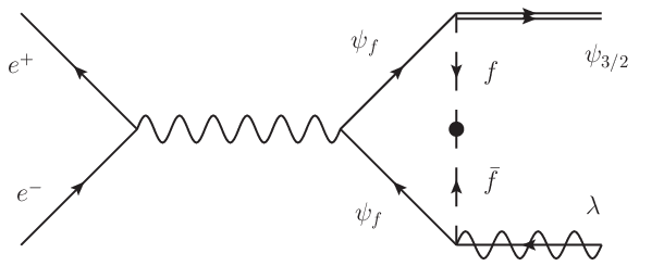

We find that the modification appears in the supergravity calculation. In GMSB models, there are messenger fields, which potentially affect the gravitino production process. In fact, they contribute to the gravitino production process through the one-loop diagrams shown in Fig. 3. Even though they are diagrams at the one-loop level, they cannot be neglected compared to the tree-level ones in Fig. 1 since the gaugino mass in Eq. (2) is at the one-loop order in GMSB models. Note here that the diagrams in Fig. 3 are not the microscopic description of the first diagram in Fig. 1. Both diagrams exist as independent ones in supergravity. The explicit calculation shows
| (13) |
where is again the -function in Eq. (10). The dots in Fig. 3 represent insertions of , and we used Eq. (8) to derive the above formula. A few comments are in order. At a lower energy than the messenger mass scale, the messenger fields can be integrated out and absent in the low energy theory. The gravitino interactions are then completely read off from the supergravity Lagrangian of the MSSM fields (1). The supergravity prediction in Eq. (2), therefore, should not be altered for . The additional contribution (13) indeed respects this consideration. The factor, , in Eq. (13) goes to zero as , and thus the amplitude is accurately represented by Eq. (2) at low energy. However, the one-loop contribution becomes comparable to that of tree-level for since the factor, , approaches to .
Combined with the tree-level contribution (2), we confirmed that the growing amplitude at in supergravity is completely cancelled by the one-loop diagrams, and the total supergravity calculation coincides with the result from global SUSY,
| (14) |
Additional contribution from the tree-level messenger scatterings
For , in addition to the scattering processes of the MSSM particles, the goldstino is also produced by scattering processes where the messenger fields are in the external lines. The reaction rate is calculated to be [20]
| (15) |
As we see from Eq. (12) and Eq. (15), the reaction rate of the messenger particles is larger than that of the MSSM particles by a loop-factor since the messenger fields directly couple to the goldstino through the superpotential interaction.
2.2 The gravitino relic abundance
Summarizing the previous subsection, in GMSB models, the gravitino is produced from the scattering processes of the MSSM fields and the messenger fields. Depending on the value of , the resultant gravitino relic abundance is determined by different values; if , the abundance is fixed by , and if , it is the messenger mass scale to fix the abundance,
| (16) | |||
| (17) |
The abundance in Eq. (17) is not a straightforward replacement of to in Eq. (16) since the production through the messenger fields are not suppressed by a loop factor.

The estimates so far do not include a contribution of the transverse mode of the gravitino. For a very high reheating temperature, the transverse mode becomes relevant,
| (18) |
Including both the longitudinal and the transverse modes, we show the gravitino relic abundance in GMSB with the messenger scale fixed to be in Fig. 4. As we see from the figure, the gravitino relic abundance is predicted to be constant in a wide range of the reheating temperature, but the amount is too large compared to the observed dark matter energy density . The overproduced gravitinos must be diluted by some mechanism. Although the prediction to is too large, the insensitivity to brings us a new scenario of gravitino DM.
3 A new scenario of gravitino dark matter
As we have confirmed in the previous section, the gravitino relic abundance becomes insensitive to once the temperature of the Universe exceeds the messenger mass scale. The results have a crucial impact on the possible mechanism of baryogenesis. In this section, we present a new cosmological scenario of gauge mediation, where gravitino dark matter and thermal leptogenesis are compatible. The scenario requires a late-time entropy release by some mechanism, which is automatically supplied by the decay of the SUSY breaking pseudo-moduli field. We demonstrate the scenario with a simple model of gauge mediation as an example and see that the scenario actually works.
Throughout the analysis, we assume the SUSY scale to be TeV and in particular fix the gluino mass to be TeV to account for the Higgs boson mass of 125 GeV within the MSSM in GMSB [3]. Although most of the SUSY particles are then too heavy to be detected at the LHC experiments, the model predicts higgsino to be as light as . We briefly mention the cosmological constraint on the light higgsino in the last subsection.

3.1 Compatibility with thermal leptogenesis
In a light gravitino scenario, thermal leptogenesis and gravitino DM are thought to be incompatible with each other. The possible maximum amount of baryon asymmetry produced by the thermal leptogenesis is proportional to the reheating temperature [15, 16, 17, 18],
| (19) |
which puts a lower bound on ( to realize the observed value . If the gravitino relic abundance is represented as Eq. (16) for any , the thermal production of gravitino DM and the thermal leptogenesis are incompatible; even if we assume a late-time entropy production to dilute overproduced gravitino to match the abundance to the observation, baryons are also diluted at the same time and the abundance never reproduces the observation. In other words, the ratio is constant as long as the abundances are both proportional to , and always larger than the observed ratio, .
However, in GMSB, if the reheating temperature is higher than the messenger mass scale, the gravitino relic abundance becomes insensitive to . Then, the observed ratio of the energy densities, , can be realized with thermally produced gravitino and the thermal leptogenesis. We plot the prediction for to visualize the situation in Fig. 5. If the gravitino abundance is proportional to for any , the theoretical prediction never reaches the observed value (dotted line). However, if the reheating temperature is higher than the messenger scale, becomes independent of in GMSB, which allows to achieve the observed value.
3.2 Late-time entropy release
The ratio of the energy densities can be realized by thermally produced gravitino and thermal leptogenesis with an appropriate reheating temperature as we saw above. However, as is obvious from Fig. 4, the predicted gravitino abundance is too large compared to the observation, . The overproduced gravitino should be diluted by a late-time entropy release by some mechanism. The required amount of dilution is
| (20) | ||||
| (21) |
where is assumed.
Actually, a source of entropy production is already incorporated in the scenario: the scalar component of the singlet superfield , which is called the pseudo-moduli field. In the early Universe, it is possible that the pseudo-moduli is displaced from the vacuum and starts oscillation around the minimum. Since the pseudo-moduli is massless at tree-level and gets mass only through the quantum effects, it is often much lighter than the SUSY breaking scale, , and is long-lived if there is a weakly coupled description for the SUSY breaking sector. In such a case, the pseudo-moduli can eventually dominate the energy density of the Universe, and a sizable amount of entropy is produced from its decay.
3.3 Demonstration in a simple model of gauge mediation
The model
We study a low-energy effective theory of O’Raifeartaigh type SUSY breaking model coupled with the messenger fields:
| (22) | ||||
| (23) |
where is a gauge singlet superfield called the SUSY breaking pseudo-moduli. The messenger superfields are demoted by and . There is an -symmetry where the charge assignment is and . If the -symmetry is unbroken, is stabilized at where we cannot integrate out the messenger fields. Once we turn on the supergravity effects, however, the -symmetry is explicitly broken by the supergravity correction represented by the constant term , which destabilizes the origin and creates the SUSY breaking vacuum at [23], where is the reduced Planck scale.
Since there is also a SUSY preserving minimum at where the messenger fields condense, the SUSY breaking vacuum is a meta-stable state. For a realistic cosmology, the field should stay away from the SUSY vacuum in the course of cosmological evolution.
Cosmological evolution of
Cosmological evolution of the pseudo-moduli in the model in Eqs. (22) and (23) is examined in detail in Refs. [25, 26, 27, 28, 29]. It has been found that the SUSY breaking minimum is preferred to the SUSY preserving one for a wide region of the parameter space even if the messenger particles enter the thermal equilibrium33 3 The vacuum selection is discussed in the literatures [30, 31, 32, 33, 34, 35, 36, 37, 38, 39]. The present model had been thought to be problematic because the field tends to fall into the SUSY preserving vacuum by a finite temperature potential. . Also, with an appropriate initial condition the pseudo-moduli start oscillation around the SUSY breaking vacuum and the oscillation energy dominates the energy density of the Universe.
We define the dilution factor due to the entropy release from the decay of the pseudo-moduli as
| (24) |
where and represent the entropy densities produced by the decays of the inflaton and , respectively. If , is well approximated by
| (25) |
where is the energy density of and is a decay temperature of the pseudo-moduli, which is defined by
| (26) |
The total decay width of is denoted as . The formulae of and are found in appendix A.
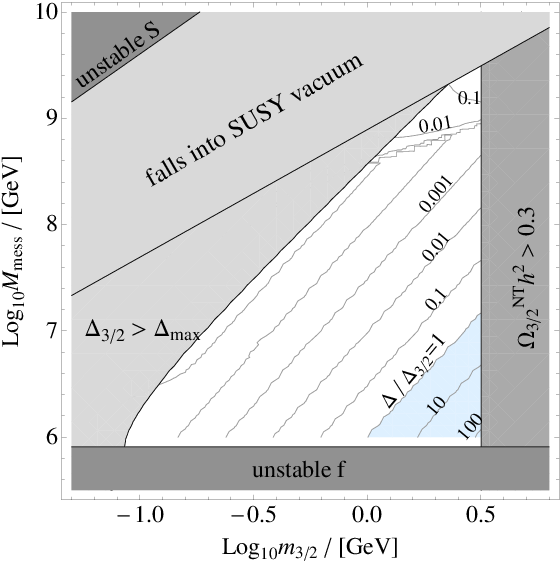
If the magnitude of dilution factor coincides in Eq. (21), the overproduced gravitinos are diluted to realize the observed dark matter abundance, . In order to realize the right amount of baryons, , at the same time, we need an appropriate reheating temperature. Since the baryon asymmetry is also diluted by the entropy production, the reheating temperature should be high enough to produce abundant baryons in advance, namely is required in the scenario. We show the required set of the dilution factor () and the reheating temperature () in vs plane in Fig. 6.
In the present set-up, there exists a parameter region where the dark matter and the baryon asymmetry are explained by thermally produced gravitino and thermal leptogenesis simultaneously (blue and green regions), with an appropriate combination of and .
In order to estimate the magnitude of the dilution factor from the decay, we numerically solved the equation of motion of the pseudo-moduli with the initial condition set at the inflaton dominated era. The results depend on the initial location of the field which can be far away from the origin depending on the inflation model and the coupling between and the inflaton [25, 26]. In this study, we choose the initial position of to be or for illustration. The results are shown in Fig. 7. As we see from the figure, by choosing an appropriate value of the initial condition of from between and , the required amount of entropy can be supplied from the oscillation energy everywhere in the blue and green regions in Fig. 6; we have confirmed that required entropy production can be obtained in this model.
Non-thermal gravitino production
While the dark matter is explained by thermally produced gravitino in the blue and green regions in Fig. 6, gravitinos are also produced non-thermally by the rare decay . We calculate the non-thermally produced gravitino abundance in appendix A and found that the abundance coincides the observed dark matter abundance with . Taking into account possible theoretical errors, we show the parameter region where is predicted as a green band in Fig. 6.


3.4 Comments on a light higgsino
So far we have studied a new cosmological scenario with a high SUSY scale in order to realize a 125 GeV Higgs boson mass. If all the SUSY particles are as heavy as 5 TeV, it is difficult to confirm the scenario by the LHC experiments. However, it is possible that the -parameter in the MSSM is much smaller than other superparticle masses. In the GMSB model we used for the cosmological study there is a natural solution to the -problem (we mention the prescription in appendix B). The model predicts a light higgsino with its mass of . The -term is generated by a direct coupling between SUSY breaking chiral multiplet and Higgs multiplets assumed at the cutoff scale , which results in a relatively small -term compared to Higgs soft mass parameters. For a cosmologically favorable region of the gravitino mass, the lightest higgsino does not decay inside the detector. In that case, searches for mono-jet processes at LHC or mono-photon ones at the ILC will be able to find the light higgsino.
One should check if a light higgsino scenario is compatible with the constraint from the BBN. If the higgsino mass is so small that the life-time becomes as long as sec, the decay may alter the abundance of the light elements. We have checked the BBN constraints in the case of and found that such a light higgsino is cosmologically safe if the gravitino is lighter than MeV. A detailed discussion is given in appendix B.
4 Summary
We re-investigated the thermal production of the gravitino in general framework of gauge mediation. Calculating the gravitino production cross section using both the goldstino Lagrangian and the supergravity one, we confirmed that the relic abundance become insensitive to the reheating temperature if the temperature of the Universe once exceeds the messenger mass scale. Inspired by this property, we presented a new cosmological scenario; the gravitino dark matter and the thermal leptogenesis are compatible, namely the ratio coincides the observation, , with an appropriate value of reheating temperature. To realize the correct absolute value of each quantity, and , a late-time entropy release is required, which is automatically supplied by the oscillation energy of the pseudo-moduli.
To make sure that the scenario actually works, we examined cosmological evolution of the pseudo-moduli field in a concrete model of gauge mediation. With an appropriate initial condition, we showed that the oscillation energy of the pseudo-moduli dominates the energy density of the Universe and a sizable amount of entropy needed to fix the energy densities of gravitino and baryon is released by the subsequent decay. The scenario is realized when the gravitino mass is and the messenger scale is .
Although we have studied the scenario with to account for the 125 GeV Higgs boson, the higgsino can be as light as . Such a light higgsino can be discovered in a future experiments. We have checked that a light higgsino is safe from the BBN constraints if the gravitino mass is smaller than 500 MeV.
Acknowledgments
We would like to thank Fuminobu Takahashi for discussions on gravitino thermal production. RK is supported in part by the Grant-in-Aid for Scientific Research 23740165 of JSPS and 25105011 of MEXT.
Appendix A Pseudo-moduli interactions with the MSSM fields
We summarize the interactions between the pseudo-moduli and the MSSM fields needed to study the decay of . The pseudo-moduli interacts with the MSSM fields through the messenger loop diagrams. The interactions can be read off from the dependence of the low energy parameters [25, 26]. For scalar fields , the effective interaction Lagrangian is written as
| (27) |
The effective mass parameter is a part of the scalar mass that is proportional to . One element of the scalar mass is the contribution from the gauge mediation,
| (28) |
which is induced at the messenger mass scale . If the gauge mediation is the only source of the scalar mass, is identical to their mass. In that case, is the gauge mediation contribution plus the radiative corrections. In appendix B, we consider a direct coupling between the field and the Higgs superfields to solve the -problem. In that case, consists of two sources; one is from the gauge mediation and the other is from the direct coupling. The latter piece does not depend on , and has little effect on the effective coupling constant.
As we evaluate the abundance of non-thermally produced higgsino to check the BBN constraint in appendix B, we list the interaction with higgsino,
| (29) |
The coefficient is again a part of that is proportional to . Actually, as we see in appendix B, -term is generated at the cutoff scale through the Khler potential Eq. (38) and it does not have dependence. The VEV dependence of appears only through the renormalization group running, and the effect is very small for the -term. The effective coupling is suppressed compared to the -term, typically
| (30) |
Among the effective couplings, the Higgs mass parameter is enhanced by the large renormalization group running [26],
| (31) |
with
| (32) |
Decays of the field
The field mainly decays into the MSSM particles. Since the mass parameter is enhanced over other SUSY breaking parameters, the decay rate into the Higgs boson is enhanced. For , the main decay channel turns out to be and , where the gauge bosons are longitudinally polarized [26],
| (33) |
Approximating the total decay width by that of main channel, the decay temperature defined in Eq. (26) is written as
| (34) |
There is also a rare decay mode , which become important if the gravitino mass is larger than . The decay width is calculated to be [25, 26]
| (35) |
If dominates the energy density of the Universe, non-thermal gravitino abundance is calculated to be
| (36) |
where is the critical density divided by the entropy density at present. Approximating the decay temperature as Eq. (34), the non-thermal gravitino is estimated as
| (37) |
We have used the formula in Fig. 6.
Appendix B -problem and a light higgsino
Here we present a possible solution to the -problem. As we see below, the solution predicts a relatively light higgsino compared to . We check whether a light higgsino scenario is allowed by the BBN constraint.
In order to avoid too large -term, we assume an approximate Peccei-Quinn (PQ) U(1) symmetry with a charge assignment . Also, to realize the relation , we assume the following general interactions between and the Higgs superfields at the cutoff scale [24],
| (38) |
where the PQ charge of is fixed as . Once the -component of develops a VEV, -term and the Higgs scalar mass terms emerge at the scale . The relation , which is needed for satisfying the condition of electroweak symmetry breaking without a serious fine-tuning, naturally realizes if the coefficients and are both .
Possible origins of the Khler potential (38) are discussed in Ref. [24] by studying dynamics of UV models above the cutoff scale . There, it is found that the coefficients and tend to have a mild hierarchy, and we typically have . This hierarchy implies that the Higgs scalar mass parameter tends to be above the order of TeV scale for a moderate value of -term, namely for .
We do not regard this small hierarchy as catastrophic; actually, this hierarchy is consistent with the relatively heavy Higgs boson mass. In order for the electroweak symmetry to be broken radiatively, the condition
| (39) |
must be satisfied. is a contribution from the radiative corrections. With positive and , must be negative and large to satisfy the condition (39), which is realized by the contributions from the stop-loop diagrams if the stop mass is large. Large stop mass subsequently induce a large contribution proportional to to the Higgs boson mass again through the stop-loop diagram to realize a relatively heavy Higgs boson. In summary, in this set-up, the -problem is ameliorated by the generalized version of the Giudice-Masiero mechanism with the Khler potential in Eq. (38), which in turn leads the relatively small -term and the relatively heavy Higgs boson mass in accord with .
Although it is difficult to discover a SUSY particles at the LHC experiments when , it predicts a light higgsino with . Therefore, in this scenario, there is a chance to discover a light higgsino in the future experiment.
The light higgsino in GMSB is subject to the constraints from BBN. The constraints on the primordial abundance of the lightest neutralino is studied in Ref. [40]. They analyzed the decay process of the neutralino and presented constraints on , the yield of , in a Bino-like NLSP case. We use the constraints to derive those for the higgsino.
Since the life-time of a neutralino is approximately proportional to , constraints on the primordial abundance are more severe for larger or smaller . We focus on a case that the mass of NLSP (in our case higgsino) is . According to Ref. [40], if the gravitino is heavier than , the stringent bound on the bino abundance comes from the overproduction of the Deuterium. For , the bound is from the overproduction of ,
| (40) | ||||
| (41) |
The bound is much weaker for . We estimate the higgsino abundance in the scenario and check whether a light higgsino is allowed by BBN.
Higgsinos are produced non-thermally from the decay of the pseudo-moduli,
| (42) |
where is the branching ratio of the decay process and the decay temperature is well approximated by Eq. (34). depends on two effective couplings : and defined in appendix A. Remaining these parameters, the higgsino abundance is estimated as
| (43) |
The abundance of the non-thermally produced higgsinos is decreased by the subsequent annihilation process. This effect can be taken into account by solving the Boltzmann equation,
| (44) |
where is the thermal averaged annihilation cross section of higgsino [41] 22 2 We have not included co-annihilation effects to make a conservative estimate. ,
| (45) |
where is Weinberg angle. The solution of the Boltzmann equation (44) is approximated by a simple analytic formula [42, 26]. In terms of the yield value ,
| (46) |
If the initial abundance produced by the decay of is large enough, the resultant abundance for is independent of . In this case, the abundance is estimated by
| (47) |
For higgsino with ,
| (48) |
Compared with Eq. (40) and (41), we see that the higgsino abundance is below the BBN constraint for with the help of the annihilation process.
References
- [1] M. Dine, W. Fischler and M. Srednicki, Nucl. Phys. B 189, 575 (1981); S. Dimopoulos and S. Raby, Nucl. Phys. B 192, 353 (1981); M. Dine and W. Fischler, Phys. Lett. B 110, 227 (1982); Nucl. Phys. B 204, 346 (1982); C. R. Nappi and B. A. Ovrut, Phys. Lett. B 113, 175 (1982); L. Alvarez-Gaume, M. Claudson and M. B. Wise, Nucl. Phys. B 207, 96 (1982); S. Dimopoulos and S. Raby, Nucl. Phys. B 219, 479 (1983).
- [2] M. Dine and A. E. Nelson, Phys. Rev. D 48, 1277 (1993) [hep-ph/9303230]; M. Dine, A. E. Nelson, Y. Nir and Y. Shirman, Phys. Rev. D 53, 2658 (1996) [hep-ph/9507378]; M. Dine, A. E. Nelson and Y. Shirman, Phys. Rev. D 51, 1362 (1995) [hep-ph/9408384].
- [3] P. Draper, P. Meade, M. Reece and D. Shih, Phys. Rev. D 85, 095007 (2012) [arXiv:1112.3068 [hep-ph]].
- [4] T. Moroi, H. Murayama and M. Yamaguchi, Phys. Lett. B 303, 289 (1993).
- [5] M. Kawasaki and T. Moroi, Prog. Theor. Phys. 93, 879 (1995) [hep-ph/9403364, hep-ph/9403061].
- [6] T. Moroi, hep-ph/9503210.
- [7] A. de Gouvea, T. Moroi and H. Murayama, Phys. Rev. D 56, 1281 (1997) [hep-ph/9701244].
- [8] M. Bolz, W. Buchmuller and M. Plumacher, Phys. Lett. B 443, 209 (1998) [hep-ph/9809381].
- [9] M. Bolz, A. Brandenburg and W. Buchmuller, Nucl. Phys. B 606, 518 (2001) [Erratum-ibid. B 790, 336 (2008)] [hep-ph/0012052].
- [10] J. Pradler and F. D. Steffen, Phys. Rev. D 75, 023509 (2007) [hep-ph/0608344].
- [11] J. Pradler and F. D. Steffen, Phys. Lett. B 648, 224 (2007) [hep-ph/0612291].
- [12] V. S. Rychkov and A. Strumia, Phys. Rev. D 75, 075011 (2007) [hep-ph/0701104].
- [13] M. Kawasaki, K. Kohri and T. Moroi, Phys. Rev. D 71, 083502 (2005) [astro-ph/0408426].
- [14] M. Fukugita and T. Yanagida, Phys. Lett. B 174, 45 (1986).
- [15] S. Davidson and A. Ibarra, Phys. Lett. B 535, 25 (2002) [hep-ph/0202239].
- [16] G. F. Giudice, A. Notari, M. Raidal, A. Riotto and A. Strumia, Nucl. Phys. B 685, 89 (2004) [hep-ph/0310123].
- [17] W. Buchmuller, R. D. Peccei and T. Yanagida, Ann. Rev. Nucl. Part. Sci. 55, 311 (2005) [hep-ph/0502169].
- [18] W. Buchmuller, P. Di Bari and M. Plumacher, Annals Phys. 315, 305 (2005) [hep-ph/0401240].
- [19] G. ’t Hooft and M. J. G. Veltman, Nucl. Phys. B 153, 365 (1979).
- [20] K. Choi, K. Hwang, H. B. Kim and T. Lee, Phys. Lett. B 467, 211 (1999) [hep-ph/9902291].
- [21] K. Jedamzik, M. Lemoine and G. Moultaka, Phys. Rev. D 73, 043514 (2006) [hep-ph/0506129].
- [22] I. Dalianis, arXiv:1304.7673 [hep-ph].
- [23] R. Kitano, Phys. Lett. B 641, 203 (2006) [hep-ph/0607090].
- [24] M. Ibe and R. Kitano, JHEP 0708, 016 (2007) [arXiv:0705.3686 [hep-ph]].
- [25] M. Ibe and R. Kitano, Phys. Rev. D 75, 055003 (2007) [hep-ph/0611111].
- [26] K. Hamaguchi, R. Kitano and F. Takahashi, JHEP 0909, 127 (2009) [arXiv:0908.0115 [hep-ph]].
- [27] H. Fukushima, R. Kitano and F. Takahashi, JHEP 1302, 140 (2013) [arXiv:1209.1531 [hep-ph]].
- [28] I. Dalianis and Z. Lalak, JHEP 1012, 045 (2010) [arXiv:1001.4106 [hep-ph]].
- [29] I. Dalianis and Z. Lalak, Phys. Lett. B 697, 385 (2011) [arXiv:1012.3157 [hep-ph]].
- [30] S. A. Abel, C. -S. Chu, J. Jaeckel and V. V. Khoze, JHEP 0701, 089 (2007) [hep-th/0610334].
- [31] N. J. Craig, P. J. Fox and J. G. Wacker, Phys. Rev. D 75, 085006 (2007) [hep-th/0611006].
- [32] W. Fischler, V. Kaplunovsky, C. Krishnan, L. Mannelli and M. A. C. Torres, JHEP 0703, 107 (2007) [hep-th/0611018].
- [33] S. A. Abel, J. Jaeckel and V. V. Khoze, JHEP 0701, 015 (2007) [hep-th/0611130].
- [34] L. Anguelova, R. Ricci and S. Thomas, Phys. Rev. D 77, 025036 (2008) [hep-th/0702168 [HEP-TH]].
- [35] C. Papineau, JHEP 0805, 068 (2008) [arXiv:0802.1861 [hep-th]].
- [36] R. Auzzi, S. Elitzur and A. Giveon, JHEP 1003, 094 (2010) [arXiv:1001.1234 [hep-th]].
- [37] A. Katz, JHEP 0910, 054 (2009) [arXiv:0907.3930 [hep-th]].
- [38] E. F. Moreno and F. A. Schaposnik, JHEP 0910, 007 (2009) [arXiv:0908.2770 [hep-th]].
- [39] A. Ferrantelli and J. McDonald, JCAP 1002, 003 (2010) [arXiv:0909.5108 [hep-ph]].
- [40] M. Kawasaki, K. Kohri, T. Moroi and A. Yotsuyanagi, Phys. Rev. D 78, 065011 (2008) [arXiv:0804.3745 [hep-ph]].
- [41] N. Arkani-Hamed, A. Delgado and G. F. Giudice, Nucl. Phys. B 741, 108 (2006) [hep-ph/0601041].
- [42] M. Fujii and K. Hamaguchi, Phys. Rev. D 66, 083501 (2002) [hep-ph/0205044].