Consensus in continuous-time multi-agent systems under discontinuous nonlinear protocols
Liu Bo, Lu Wenlian and Chen Tianping
School of Mathematical Sciences, Fudan University, Shanghai, 200433, P.R.China.
In this paper, we provide a theoretical analysis for nonlinear discontinuous consensus protocols in networks of multiagents over weighted directed graphs. By integrating the analytic tools from nonsmooth stability analysis and graph theory, we investigate networks with both fixed topology and randomly switching topology. For networks with a fixed topology, we provide a sufficient and necessary condition for asymptotic consensus, and the consensus value can be explicitly calculated. As to networks with switching topologies, we provide a sufficient condition for the network to realize consensus almost surely. Particularly, we consider the case that the switching sequence is independent and identically distributed. As applications of the theoretical results, we introduce a generalized blinking model and show that consensus can be realized almost surely under the proposed protocols. Numerical simulations are also provided to illustrate the theoretical results.
Key words: multiagent systems, consensus, discontinuous, switching, almost sure
1 Introduction
In many applications involving multiagent systems, groups of agents are required to agree upon certain quantities of interest. This is the so-called “consensus problem”. Due to the broad applications of multiagent systems, consensus problem arises in various contexts such as the swarming of honeybees, flocking of birds (Olfati-Saber, 2006), formation control of autonomous vehicles (Fax & Murray, 2004), distributed sensor networks (Cortés & Bullo, 2005) and so on. In the past decades, a considerable research effort has been devoted to this problem. Various consensus algorithms have been proposed and studied. For a review, see the survey Olfati-Saber, Fax & Murray (2007), Ren, Beard, & Atkins (2005) and references therein.
Most existing consensus protocols are continuous protocols, i.e., the protocol are continuous functions of time and the states of the agents. For example, in Olfati-Saber & Murray (2004), the authors studied the following linear consensus protocols:
where is the state of the -th agent at time , and is the set of neighbors of agent . In Liu, Chen, & Lu (2009), the authors studied two types of nonlinear protocols over directed graphs. The first one is as follows:
| (1) |
where are nonlinear functions satisfying the following assumption:
Assumption 1.
- 1.
are locally Lipschitz continuous;
- 2.
if and only if ;
- 3.
, .
They prove that this protocol can realize consensus if and only if the underlying graph has a spanning tree. The second one is as follows:
| (2) |
where is a strictly increasing nonlinear function, and the Laplacian matrix has the form
where , is irreducible, and . They prove that this protocol can realize consensus value which is a convex combination of component states of the initial value.
Previous protocols are for static networks, i.e., networks with fixed topologies. Yet many real world networks are not static. For example, in a network of mobile agents, the topology of the network is dynamical due to limited transmission range and the movement of the agents. In some cases, the network topology changes gradually. In other cases, it changes abruptly, which induces discontinuity in the network topology.
An important class of discontinuous dynamical network topology is the so-called switching topology. Let be a partition of , on each time interval , the network has a fixed topology, while at each time point , the topology switches to another one randomly or according to some given rule. Linear consensus protocols over networks with stochastically switching topologies such as independent and identically distributed switching (Salehi & Jadbabaie, 2007), Markovian switching (Matei, Martins, & Baras, 2008), and adapted stochastic switching (Liu, Lu, & Chen, 2011) have been studied and conditions for almost sure consensus have been obtained, which indicates that a directed spanning tree in the expectation is sufficient for almost sure consensus.
The above mentioned discontinuous consensus protocols are discontinuous in time and continuous in the states of the agents. Besides, there are another important class of discontinuous consensus protocols which are discontinuous in the states of the agents, too. Recently, such protocols have been discussed in several papers. In Cortés (2006), based on normalized and signed gradient dynamical systems associated with the Laplacian potential, the author proposed the following two discontinuous consensus protocols:
| (4) | |||
| (5) |
where is the graph Laplacian of the underlying graph, and . Finite time convergence of both protocols on connected undirected graphs was proved, where the centralized protocol (4) can realize average consensus, while the distributed algorithm (5) can reach average-max-min consensus. In Cortés (2008), the author further considered the following two discontinuous protocols:
| (6) | |||
| (7) |
where if and if , if and if . Both protocols can realize finite time consensus in a strongly connected weighted directed graph, where protocol (6) can reach max consensus, while protocol (7) can reach min consensus. In Hui, et al. (2008), the author studied the stability of consensus under the following discontinuous protocol:
Under the assumption that is symmetric and , they proved finite time convergence for this protocol.
In this paper, we investigate a new type of nonlinear discontinuous protocols, which can be formulated as follows:
where is the underlying graph Laplacian, and is a discontinuous function that will be specified later. First, we consider networks with fixed topology. Compared to existing works which only consider connected undirected graphs or strongly connected directed graphs, we consider more general directed graphs that has spanning trees. We show that a directed spanning tree is sufficient for the network to realize asymptotic consensus. And this condition is not only sufficient but also necessary. This is an important improvement since directional communication is important in practical applications and can be easily incorporated, for example, via broadcasting. Moreover, a lot of important real world networks such as the leader-follower networks are not strongly connected. Then, motivated by the work in synchronization analysis by Lu and Chen (2004), we locate the consensus value based on the left eigenvector corresponding to the zero eigenvalue of the graph Laplacian. Finally, we show that if the consensus value is a discontinuous point of , and the underlying graph is strongly connected, then finite time convergence can be realized.
We also consider the consensus protocol over networks with switching topologies. The time interval between each successive switching is assumed to be an independent and identically distributed random variable. And the network topology is also a random sequence. We prove a sufficient condition for the network to achieve consensus almost surely in terms of the scramblingness of the underlying graph. Based on this result, we study the special case where the switching sequence is independent and identically distributed. We show that if the underlying graph has a positive probability to be scrambling, then the protocol can realize consensus almost surely. Our results indicate that for a network with stochastically switching topology to reach consensus almost surely, the network is unnecessary connected at each time point. This is more general than the work in Hui, et. al.(2008) on network with switching topology.
Finally, as applications of the theoretical results. We study consensus in a general blinking network model under the proposed consensus protocol. Numerical simulations are also provided to illustrate the theoretical results.
This paper is organized as follows. In Section 2, some preliminary definitions and lemmas concerning graph theory, matrix theory nonsmooth analysis, and probability, are provided. Consensus analysis under nonlinear discontinuous protocols with both fixed topology and switching topology, are carried out in Section 3. An application of the theoretical results to a general blinking network model with numerical simulations are given in Section 4. The paper is concluded in Section 5.
2 Preliminaries
In this section, we present some definitions and basic lemmas that will be used later.
2.1 Algebraic graph theory and matrix theory
A weighted directed graph of order is denoted by a triple where is the vertex set and is the edge set, i.e., if there is an edge from to , and , , is the weight matrix which is a nonnegative matrix such that for , if and only if and . For a weighted directed graph of order , the graph Laplacian can be defined from the weight matrix in the following way:
And for a given Laplacian matrix , the weighted directed graph corresponding to is written as .
In this paper, we only consider simple graphes, i.e., there are no self links and multiple edges. A directed path of length from to is an ordered sequence of distinct vertices with and such that . A (directed) spanning tree is a directed graph such that there exists a vertex , called the root vertex, such that for any other vertex , there exists a directed path from to . We say a graph has a spanning tree if a subgraph of that has the same vertex set with is a spanning tree. A graph is strongly connected if for any pair of vertices, say, , , there exist directed paths both from to and from to .
If a graph has spanning trees, then the vertices of the graph can be divided into two disjoint sets: , , where contains the vertices that can be the root of some spanning tree, contains all other vertices. We have the following lemma.
Lemma 1.
If a graph of vertices has spanning trees, let , be defined as above, then
- (i)
The subgraph of induced by is strongly connected.
- (ii)
is strongly connected if and only if .
Proof: (i): First, for any given vertices , since can be the root of some spanning tree, then from definition, there is a directed path from to . On the other hand, can also be the root of some spanning tree, so there also exists a directed path from to . Second, we prove that these two paths contain no vertices outside . Otherwise, there exists a vertex such that is on one of the paths. Suppose is on the path from to , then there is a directed path from to . Since is a root, there exist directed paths from to all other vertices. Thus there are directed paths from to all other vertices, which implies also can be the root of some spanning tree. This contradicts the fact that .
(ii): If , then the subgraph induced by is itself. From (i), is strongly connected. On the other hand, if is strongly connected, from definition, each vertex can be the root of some spanning tree. Thus, .
Remark 1.
It is known that in a leader-follower system, only the leader can influence the follower, but the follower can not influence the leader. So the final state of the system is determined only by the leader. In a strongly connected system, each agent can be seen as a leader. So the final state of the system is determined by all agents. Yet there are also many intermediate cases between these two extremes. In such cases, there are group of leaders, but the whole system is not strongly connected. Lemma 1 unifies these three cases into a general framework.
From the proof of Lemma 1, we can see that there exist no edges from vertices of to vertices of . then after a proper renumbering of its vertices, the graph Laplacian of can be written in the following form:
where the square submatrix corresponds to the vertex set . Since the subgraph induced by is strongly connected, is irreducible. By Perron-Frobenius theory, the left eigenvector of corresponding to the eigenvalue is positive. Thus we can define the following
Definition 1.
(Weighted root average) Let be the graph Laplacian of some weighted directed graph . Suppose that has spanning trees and is of the form (2.1). Let be the positive left eigenvector of corresponding to the eigenvalue such that , where . Given some , the weighted root average of with respect to is defined as:
Remark 2.
In a leader-follower system, the final state of the system is determined by the leader only. In the case that there are group of leaders, the final state of the system is determined by the leader group. The weighted root average is also a generalization from the case of one leader to the case of leader group.
Example 1.
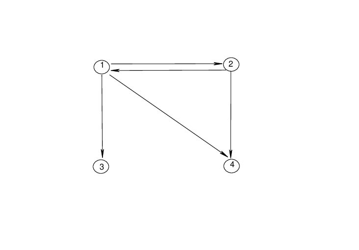
Consider the graph in Fig. 1, it is obvious that , . If we take all the positive weight of the edges to be , then the graph Laplacian is
Here, , and . Thus, for any , .
A Metzler matrix is a matrix that has nonnegative off-diagonal entries. It is clear that is a Metzler matrix with zero row sum. Following Liu and Chen (2008), for a Metzler matrix , we define a function
and we say that is scrambling if . It is obvious that scramblingness is not influenced by the diagonal entries of a Metzler matrix, so is scrambling if and only if is scrambling. On the other hand, since there is a one to one correspondence between each weighted directed graph and its weight matrix (or Laplacian matix ), we also say a graph is scrambling if (or ) is scrambling.
Remark 3.
It can be seen from the definition that if a graph is scrambling, then for each vertex pair , either there exists at least one directed edge between and , or there is another vertex such that there are directed edges from to and to . From this, it can be seen that the graph in Fig. 1 is scrambling. Since there exists directed edges between , , , and . And there exist edges from to , , and edges from to , .
If we incorporate a positive threshold on the graph , then we get the concept of -graph (Moreau, 2004). The -graph of is a graph that has the same vertex set and weight matrix with . Yet for each , , there is a directed edge from to if and only if . We say a graph is -scrambling if its -graph is scrambling.
Remark 4.
It is obvious that if is -scrambling, then .
2.2 Nonsmooth stability analysis
In this subsection, we will provide some concepts and lemmas concerning nonsmooth stability analysis. First, we present some basic concepts and theorems from Filippov theory on differential equations with discontinuous righthand sides. For more details, the readers are referred to Filippov (1988) directly.
Consider the following differential equations:
| (13) |
where , and : is a discontinuous map. Then the Filippov solution of (13) can be defined as:
Definition 2.
An absolutely continuous function : is said to be a Filippov solution to (13) on if it is a solution of the differential inclusion:
| (14) |
where is the closure of the convex hull of , is the open ball centered at with radius , and denote the usual Lebesgue measure in .
For the simplicity of notation, we denote , and (14) can be rewritten as:
| (15) |
A Filippov solution of (15) is a maximum solution if its domain of existence is maximum, i.e., it can not be extended any further. A set is weakly invariant (resp. strongly invariant) with respect to (15) if for each , contains a maximum solution (resp. all maximum solutions) from of (15).
Let : , then the usual one-sided directional derivative of at in direction is defined as:
| (16) |
The generalized directional derivative of at in direction is defined as:
| (17) |
Definition 3.
(Clarke,1983) Let : , is said to be regular at if for all , the usual one-sided directional derivative exists, and .
Following lemma can be used to derive regularity.
Lemma 2.
(Clarke,1983) Let : be Lipschitz near , then
- 1.
If is convex, then is regular at ;
- 2.
A finite linear combination (by nonnegative scalars) of functions regular at is regular at .
From Rademacher’s Theorem (Clarke,1983), we know that locally Lipschitz functions are differentiable almost everywhere.
Definition 4.
(Clarke,1983) Let : be a locally Lipschitz continuous function. Let be the set of points where fails to be differentiable, then the Clarke generalized gradient of at is the set
| (18) |
where can be any set of zero measure. The set-valued Lie derivative of with respect to (15) at is:
| (19) |
The following lemma shows that the evolution of the Filippov solutions can be measured by the Lie derivative.
Lemma 3.
Let : be a Filippov solution of (13). Let : be a locally Lipschitz and regular function. Then, is absolutely continuous, exists a.e. and for a.e. .
In the following we first define a special class of discontinuous functions which will be used throughout this paper.
Definition 5.
(Function class ) A function : belongs to , denoted by , if :
- 1.
is continuous on except for a set with zero measure, and on each finite interval, the number of discontinuous points of is finite.
- 2.
On each interval where is continuous, is strictly increasing;
- 3.
If is a discontinuous point of , let , , then .
Example 2.

Definition 6.
(shrinking condition) An absolutely continuous function : is shrinking if is nonincreasing and is nondecreasing with respect to . Furthermore, is completely shrinking£¬ if is shrinking and
Remark 5.
It is obvious that if is shrinking, then the limits of and exist as .
Definition 7.
(Aubin & Frankowska, 1990) Let , be metric spaces, A map defined on is called a set-valued map, if to each , there corresponds a set . A set-valued map is said to be upper semicontinuous at if for any opening set containing , there exists a neighborhood of such that . is said to have closed (convex, compact) image, if for each , is closed (convex, compact, respectively).
Definition 8.
(Filippov, 1988) A set valued map : is said to satisfy the basic conditions in a domain if for any , is non-empty, bounded, closed and convex, and is upper semicontinuous in .
As to the existence of Filippov solutions, we have the following
Lemma 4.
(Filippov,1988) If a set-valued map satisfies the basic conditions in the domain , then for any point , there exists a solution in of the following differential inclusion:
| (23) |
over an interval for some . Moreover, if satisfies the basic conditions in a closed bounded domain , then each solution of the differential inclusion (23) lying within can be continued either unboundedly as increases (and decreases), i.e., as , or until it reaches the boundary of the domain .
Lemma 5.
(Filippov,1988) Let a set-valued map be upper semicontinuous on a compactum and let for each the set be bounded, then is bounded on .
Remark 6.
It is clear from lemma 5 that if satisfies the basic conditions on some compact set , then is bounded on .
Lemma 6.
(Filippov,1988) If is a bounded closed set and if a function is continuous, then the set is closed. If is convex, , then the set is convex.
Remark 7.
It can be seen from lemma 6 that if a set-valued map satisfies the basic condition, then for any matrix , the set-valued map also satisfies the basic condition.
The following lemma is a generalization of LaSalle invariance principle for discontinuous differential equations.
Lemma 7.
(Cortés, 2006) Let : be a locally Lipschitz and regular function, let where is compact and strongly invariant with respect to (13). Assume that either or for all . Let . Then, any solution starting from converges to the largest invariant set contained in .
2.3 Probability theory
Let denote the probability, and be the mathematical expectation. The following are the second Borel-Cantelli Lemma concerning an independent sequence.
Lemma 8.
(Durrett, 2005) If the events are independent, then implies , where i.o. means infinitely often.
3 Consensus analysis
In this section, we will discuss consensus in a network under nonlinear discontinuous protocols with both fixed topology and switching topologies.
3.1 Consensus in networks with fixed topology.
Consider the following consensus protocol in a network of multiagents with fixed graph topologies:
| (24) |
where and is the graph Laplacian.
Denote with , then we can define a set-valued map , with , where if is continuous at , and otherwise. Since for any , the set is closed and convex, from Lemma 6, is a closed convex set. The Filippov solution to (24) is defined as the following differential inclusion:
| (25) |
First, we have the following lemma which says that all the Filippov solutions of (24) is shrinking.
Lemma 9.
For any initial value , the Filippov solution exists and is shrinking, thus, all the solutions can be extended to .
Proof: It is clear that the set-valued map satisfies the basic conditions on any bounded region of , which implies that for any initial value , the Filippov solution exists on the interval for some .
Denote , . It is easy to see that is locally Lipschitz and convex. In fact, for , , and , we have
and
Therefore, is regular and
where is the set-valued Lie derivative of with respect to .
We will prove that is nonincreasing and is nondecreasing. Here, we only show that is nonincreasing, and a similar argument can apply to .
Now, we will prove that for each , either or . Given , let . We have . If , then there exists some such that for each . Therefore, for .
Noting
for some , if is continuous at , then for , and for . So in this case we have . Otherwise, is discontinuous at . If , then for each , . Let be one index satisfying . Then we obviously have , which is a contradiction. So in this case we also have .
From Lemma 3,
Thus is nonincreasing. A similar argument can show that is nondecreasing. So is shrinking. The second claim then directly follows from Lemma 4.
Theorem 1.
The system (24) will achieve consensus for any initial value if and only if the graph of has spanning trees. And the consensus value is . Furthermore, if the graph of is strongly connected, and is discontinuous at , then finite time convergence can be achieved.
Proof: See Appendix A.
It can be seen that Theorem 1 is quite similar to the result obtained in literature for continuous consensus protocols. So the protocol (24) can be seen as natural extensions of the continuous protocols. Intuitively, if a networks has spanning trees, then the information from the roots can be sent to all other nodes in the network. And the roots can exchange information with each other. So the network can finally reach a consensus. If a network has no spanning trees, from the proof of Theorem 1, there are two possible cases. Case I: there exists an isolated subgraph that has no connection with other parts of the network. In this case the isolated subgraph can not exchange information with other parts of the network, and consensus can not be reached. Case II: there are no isolated subgraphs. In this case, the network has a subgraph that has spanning trees. There are edges from nodes outside this subgraph to nodes of this subgraph which are not roots. Fig. 5 provides an example. In this case, the roots in the subgraph can not exchange information with nodes outside the subgraph, since they can neither send their information to the nodes outside the subgraph, nor receive information from nodes outside the subgraph. As a result, consensus also can not be reached. In the following, we will provide some examples to illustrate the theoretical results.
Example 3.
The graph shown in Fig. 3 may be called a “double-star” graph. It has spanning trees, with being the set of roots. Yet this graph is not strongly connected. If we take the weight of each edge to be , then the graph Laplacian is
with , , and being the identity matrix. For any , . The simulation result is provided in Fig. 4, where is given in Example 2, and the initial value is randomly chosen. The position of is labeled on the right side with a ‘+’. It can be seen that the agents finally reach a consensus on .


Example 4.
Fig. 5 provides an example of a graph that has no spanning trees. This graph has no isolated subgraphs. The subgraph induced by has spanning trees, with being the root set. And there are edges from to . So this graph belongs to the second case discussed above. And it can not reach a consensus for arbitrary initial value. For each edge, we take the weight as . Then the graph Laplacian is
The simulation results are presented in Fig. 6, with being given in Example 2. It can be seen that no consensus is realized.


3.2 Consensus in networks with randomly switching topologies
In this section, we will investigate consensus in networks of multiagents under nonlinear protocols over graphes with randomly switching topologies.
Consider the following dynamical system:
| (28) |
where and is the graph Laplacian for the underlying graph on the time interval . At each time point there is a switching of the network topology. We consider the case that is a random sequence. Denote , in this following, we make
Assumption 2.
- 1.
is independent and identically distributed;
- 2.
the sequence and are independent;
- 3.
is uniformly bounded.
Assumption 3.
There exists such that for any with and is continuous at , , it satisfies that
Remark 8.
It is easy to verify that under Assumption 3, for any with and , , it satisfies that
First, we will prove the following Theorem for almost sure consensus.
Theorem 2.
Proof: See Appendix B.
From Theorem 2, we can have the following corollary concerning switching sequence which is independent and identically distributed.
Corollary 1.
4 Applications to a generalized blinking model
In this section, we will show how the theoretical results can be applied to analyze real world network models. For this purpose, we consider a generalized blinking network model.
The original blinking model was proposed in Belykh, Belykh, & Hasler (2004). It is a kind of small world networks that consists of a regular lattice of cells with constant nearest neighbor couplings and time dependent on-off couplings between any other pair of cells. In each time interval of duration each time dependent coupling is switched on with a probability , and the corresponding switching random variables are independent for different links and for different times. It is a good model for many real-world dynamical networks such as computers networked over the Internet interact by sending packets of information, and neurons in our brain interact by sending short pulses called spikes, etc.
On the other hand, this model is still quite restrictive in several aspects. First, this model is an undirected model. Second, the duration between any two successive switchings may not be identical, nor may it be small sometimes. And it may even be not deterministic, but just a random variable. Finally, the basic regular nearest neighbor coupling lattice may not exist, or we can say in such case.
Based on the above analysis, we make the following generalizations on the original blinking model. First, we assume the model to be a directed graph. For every two vertices , that have random switching links between them, the switching of the edge from to is independent of that from to . Second, we assume the duration between every two successive switchings is a random variable, and each duration is independent of others. Finally, we assume that may be zero in the basic nearest neighbor lattice. That is, no links exist with probability .
It is obvious that in this generalized model, the sequence of the durations are independent and identically distributed. And the underlying graph sequence is also independent and identically distributed. For each , since different links are switched on independently, it is obvious that there is a positive probability that is a complete graph. Since a complete graph is scrambling, if we set the weight of each link to be , then is -scrambling for some with a positive probability. From Corollary 1, we can see that the discontinuous consensus protocol (28) will realize consensus almost surely on a generalized blinking model.
In the simulation, we choose a network with nodes, , , and the weight of each link to be . The duration between every two successive switching is a random variable uniformly distributed on . Let be as given in Example 2. The initial value is chosen randomly. The simulation results are presented in Fig. 7. It can be seen that consensus can be reached almost surely.

5 Conclusion
In this paper, we investigate consensus in networks of multiagents under nonlinear discontinuous protocols. First, we consider networks with fixed topology described by weighted directed graphs. Compared to existing results concerning discontinuous consensus protocols, we do not require the underlying graph to be strongly connected. Instead, we prove that a directed spanning tree is sufficient and necessary to realize consensus. And we can also locate the consensus value. This result can be seen as an extension of continuous protocols if we take continuous protocols as special case of discontinuous ones. Under this viewpoint, we establish a more generalized theoretical framework for consensus analysis. Second, we consider networks with randomly switching topologies. We provide sufficient conditions for the network to achieve consensus almost surely based on the scramblingness of the underlying graphs. Particularly, we consider the case when the switching sequence is independent and identically distributed. Compared to existing results on discontinuous protocols, we do not require the network to be connected at each time point. Finally, as application of the theoretical results, we study a generalized blinking model and show that consensus can be realized almost surely under the proposed discontinuous protocols.
References
-
Aubin, J., Frankowska, H. (1990). Set-valued analysis, Boston: Birkhauser.
-
Belykh, I., Belykh, V., & Hasler, M. (2004). Blinking model and synchronization in small world networks with a time-varying coupling, Physica D, 195, 188-206.
-
Clarke, F. (1983). Optimization and nonsmooth analysis, New York: Wiley.
-
Cortés, J. (2006). Finite-time convergent gradient flows with applications to network consensus, Automatica, 42, 1993-2000.
-
Cortés, J. (2008). Distributed algorithms for reaching consensus on general functions, Automatica, 44, 726-737.
-
Cortés, J., & Bullo, F. (2005). Coordination and geometric optimization via distributed dynamical systems, SIAM Journal on Control and Optimization, 44, 1543-1574.
-
Durrett, R. (2005). Probability: Theory and Examples, 3rd ed. Belmont, CA: Duxbury Press.
-
Fax, A., & Murray, R. (2004). Information flow and cooperative control of hehicle formations, IEEE Transactions on Automatic Control, 49, 1465-1476.
-
Filippov, A. (1988). Differential equations with discontinuous righthand sides, Kluwer.
-
Hui, Q., Haddad, W., & Bhat, S. (2008). Semistability theory for differential inclusions with applications to consensus problems in dynamical networks with switching topology, 2008 American Control Conference, 3981-3986.
-
Liu, B., & Chen, T. (2008). Consensus in networks of multiagents with cooperation and competetion via stochastically switching topoloiges, IEEE Transactions on Neural Networks, 19, 1967-1973.
-
Liu, B., Lu, W., & Chen, T. (2011). Consensus in networks of multiagents with switching topologies modeled as adapted stochastic processes, SIAM Journal on Control and Optimization, 49, 227-253.
-
Liu, X., Chen, T., & Lu, W. (2009). Consensus problem in directed networks of multi-agents via nonlinear protocols, Physics Letters A, 373, 3122-3127.
-
Lu, W., & Chen, T. (2004). Synchronization of coupled connected neural networks with delays, IEEE Transactions on Circuits and Systems-I, 51, 2491-2503.
-
Matei, I., Martins, N., & Baras, J. (2008). Almost sure convergence to consensus in Markovian random graphs, Proceedings of the 47th IEEE Conference on Decision and Control, Cancun, Mexico, 3535-3540.
-
Moreau, L. (2004). Stability of continuous-time distributed consensus algorithms, 43rd IEEE Conference on Decision and Control, 3998-4003.
-
Olfati-Saber, R. (2006). Flocking for multi-agent dynamical systems: Algorithms and theory, IEEE Transactions Automatic Control, 51, 401-420.
-
Olfati-Saber, R., Fax, J., & Murray, R. (2007). Consensus and cooperation in networked multi-agent systems, Proceedings of IEEE, 95, 215-233.
-
Olfati-Saber, R., & Murray, R. (2004). Consensus problems in networks of agents with switching topology and time delays, IEEE Transactions on Automatic Control, 49, 1520-1533.
-
Ren, W., Beard, R., & Atkins, E. (2005). A survey of consensus problems in multi-agent coordination, Proceedings of the American Control Conference, Holland, OR, 1859-1864.
-
Salehi, A. & Jadbabaie, A. (2007). Necessary and sufficient conditions for consensus over random independent and identically distributed switching graphs, Proceedings of the 46th IEEE Conference on Decision and Control, 4209-4214.
Appendix A Proof of Theorem 1
Sufficiency: Let , where and are defined as in lemma 9. Then is locally Lipschitz and regular.
Given any initial value , denote , , and . By lemma 9, is strongly invariant. Let and be the largest weakly invariant set contained in . By Lasalle Invariance Principle (see Lemma 7), we have
where is the positive limit set of .
Let be the consensus manifold, we claim that (.) . Otherwise, there exists such that and
which means that for some with and , and
Let , and . First, from the monotonicity of , we have that and . For , we have
This implies that for all . By induction arguments it can be seen that the root set of the spanning trees is contained in . A similar argument reveals that the root set of spanning trees are contained in . But from the assumption that , we can obviously have that , which is a contradiction.
Based on previous derivation, we proved that . Next, we will show that only contains one point. Otherwise, there exist , , . Assume . Then there exists a sequence as such that . By the fact that is nondecreasing, we have , which implies . A contradiction.
Summing up, we have proved that for some . This completes the proof of the sufficiency.
Necessity: Let be the graph of , if doesn’t have a spanning tree, then there is a subgraph of that is a maximum spanning tree, i.e., if there exists a subgraph of that is a spanning tree and contains , then . Let be the vertex set of , and . Then, . Let be the set of roots of , and let . Obviously, the following properties hold:
- 1.
There are no edges from to .
- 2.
There are no edges from to .
Here, for two vertex sets, an edge from one to the other means an edge from some vertex in the former to some vertex in the latter.
Then there are two cases to be considered. For simplicity, we denote each vertex by index, and the vertex should be renumbered if necessary.
- 1.
.
In this case, after proper renumbering, from the above mentioned two properties, the matrix has the following form: , where , correspond to , , respectively. Let be the dimension of and with , then obviously, is a solution which can not achieve any consensus.
- 2.
.
In this case, after proper renumbering, from the above mentioned two properties, the matrix has the following form: , where , , correspond to , , , respectively, and “*” can be anything. Let be the dimensions of for . Let for some and , then we have for . Therefore, for any solution starting from , it holds that
no consensus will be achieved.
At last, we prove the consensus value is . Suppose that has spanning trees, and is of the following form
where corresponds to the vertex set of all the roots of the spanning trees. In such case, we have that .
Let be the eigenvector corresponding to the zero eigenvalue of . Assume , and let , then for almost all ,
where . This implies that . Since , we have . thus .
At last, we prove finite time convergence when is discontinuous at . Denote , and let . For , define a function
where is the positive left eigenvector corresponding to the zero eigenvalue of such that . Then it is obvious that , if and only if for each . Furthermore, since is strictly increasing, and , , is convex, thus regular. Also, is locally Lipschitz. So from Lemma 3, exists for a.e. , and
Since from definition, , if , then either is continuous at each , or there exists , such that for each satisfying is discontinuous at . Then let be such that , , and for each satisfying is discontinuous at , we have
where , is the second largest eigenvalue of , , and with . The last inequality is due to the fact that largest eigenvalue of is with the coresponding eigenspace being , . Since the graph of is strongly connected, is irreducible, so . Let be the index such that , and be the index such that . In the case that , we have . Otherwise, either or . If , then . If , then . These all contradict the fact that is constant. Thus . On the other hand,
Thus, we have
for . This implies that will converge to zero in finite time upper bounded by . The proof is completed.
Appendix B Proof of Theorem 2
Let , and be defined as in the previous section. Given any initial value and any switching sequence of time points, denoted by , we can construct the solution in the following way. First, with initial value , there exists a Filippov solution on some interval . By similar arguments used in the proof of Lemma 9, we can prove that is shrinking and can be extended to the whole interval . Repeating such arguments, we can show that a solution of (28) can be defined as follows:
where is a Filippov solution successively defined from on such that . It is obvious that is shrinking and absolutely continuous. Let , be the indices satisfying , , respectively. Similar to the arguments in previous section, on each interval , we have
| (33) | |||||
where for each . Therefore, we have
| (34) |
Thus if , then
| (35) |
On the other hand, let denote the space of strictly increasing infinite sequence of the natural numbers, we have
| (36) | |||||
| (37) | |||||
| (38) | |||||
Due to the independence of and from Assumption 2, we can have the equality from (36) to (37). Since is independent and identically distributed, the subsequence is also independent and identically distributed for each . From the strong law of large numbers, we have
almost surely, which implies
This implies
and
because is nonincreasing with respect to , we conclude
Theorem 2 is proved completely.