Relativistic recoil effects to energy levels in a muonic atom: a Grotch-type calculation of the second-order vacuum-polarization contributions

Savely G. Karshenboim Email: savely.karshenboim@mpq.mpg.de Affiliation: Max-Planck-Institut für Quantenoptik, Garching, 85748, Germany Affiliation: Pulkovo Observatory, St.Petersburg, 196140, Russia Evgeny Yu. Korzinin Affiliation: D. I. Mendeleev Institute for Metrology, St.Petersburg, 190005, Russia Vladimir G. Ivanov Affiliation: Pulkovo Observatory, St.Petersburg, 196140, Russia

Abstract

Adjusting a previously developed Grotch-type approach to a perturbative calculation of the electronic vacuum-polarization effects in muonic atoms, we find here the two-loop vacuum polarization relativistic recoil correction of order $\alpha^{2}(Z\alpha)^{4}m^{2}/M$ in light muonic atoms. The result is in perfect agreement with the one previously obtained within the Breit-type approach. We also discuss here simple approximations of the irreducible part of the two-loop vacuum-polarization dispersion density, which are applied to test our calculations and could be useful for other evaluations with an uncertainty better than 1%.

pacs

12.20.-m, 31.30.J-, 36.10.Gv, 32.10.Fn

I Introduction

High-precision tests of any advanced atomic calculations are possible only for few-body systems and their accuracy is going down dramatically when we increase the number of particles involved. The highest accuracy has been achieved for two-body (hydrogen-like) atomic systems. To study such systems not only are binding effects and QED loops important but also recoil effects. While the non-relativistic two-body problem is easily solved by introducing the reduced mass, the relativistic recoil effects are more complicated.

The problem of relativistic recoil effects was resolved for the pure Coulomb two-body system a long time ago. The possible solutions included the Breit equation (see, e.g., [2]) and its expansions as well as the Grotch equation [3]. For non-Coulomb systems only the Breit-type approach has successfully been used to date.

The purpose of this paper is to develop a method suitable for a calculation of a certain class of corrections of order $\alpha^{2}(Z\alpha)^{4}m^{2}/M$ . The approach is applicable to medium- $Z$ muonic and antiprotonic atoms, i.e. to the atoms whose characteristic atomic momentum $Z\alpha m$ is comparable to the electron mass $m_{e}$ . In such atoms the recoil effects are more important than in ordinary (electronic) atoms. Meanwhile the electronic vacuum polarization (eVP) effects are also enhanced. Thus a calculation of relativistic recoil eVP corrections is important. Here we calculate such corrections to the energy levels in the second order of eVP effects, which are of order $\alpha^{2}(Z\alpha)^{4}m^{2}/M$ .

This papers is the third paper of the series [4, 5] devoted to a general approach to calculate relativistic recoil effects and its applications. In these papers, as explained in the first paper of the series [4], we develop an approach which can be applied for a certain class of potentials (or rather to a certain class of corrections to the interaction between the atomic particles). While the expressions are valid for a certain range of atoms for arbitrary states, the practical importance of the corrections depends on the value of the nuclear charge, the atomic weight of the nucleus, the mass of the orbiting particle (which is indeed different for muons and antiprotons) and the transition between what levels are studied and with what accuracy.

At this stage we are interested in deriving the method and its verification, rather than in its application to any particular transition of practical interest. Below we derive the general equations that take into account second-order-eVP relativistic recoil effects. For the verification of the method we choose to calculate the corrections which are known from a calculation with an alternative (Breit-type) technique in our previous paper [6].

Generalizing the method, developed by Grotch and Yennie [3] to evaluate of the relativistic recoil effect in pure Coulomb systems, to effects of eVP in muonic atoms, in [4, 5] we derived the general expression

$\displaystyle E$	$\displaystyle=$	$\displaystyle m+m_{R}(f_{CN}({Z\alpha},Z\alpha m_{R}/m_{e})-1)$	(1)
	$\displaystyle-$	$\displaystyle\frac{m_{R}^{2}}{2M}\left(f_{CN}({Z\alpha},Z\alpha m_{R}/m_{e})-1\right)^{2}$
	$\displaystyle-$	$\displaystyle\frac{m_{R}^{2}}{2M}\frac{\partial}{\partial\ln\kappa}\left(f_{CN}({Z\alpha},\kappa)-1\right)^{2}\Bigg\|_{\kappa=Z\alpha m_{R}/m_{e}}$
	$\displaystyle-$	$\displaystyle\langle\psi_{C}\|\left(\frac{V^{2}}{2M}+\frac{1}{4M}[V,[\mathbf{p}^{2},W]]\right)\|\psi_{C}\rangle\,,$

which is valid for an arbitrary perturbed potential

V=V_{C}+V_{N}\,,

where $V_{C}$ is the Coulomb potential and in a certain sense $V_{N}$ is smaller than $V_{C}$ , i.e. $V_{N}\sim\varepsilon V_{C}$ , $\varepsilon\ll 1$ . It is important that $V_{N}$ is a kind of nonrelativistic potential in the sense that its leading nonrelativistic contribution to the energy is of order $\varepsilon(Z\alpha)^{2}m$ , while the first relativistic correction appears in order $\varepsilon(Z\alpha)^{4}m$ .

Here, $W$ is a specific auxiliary potential, $\psi_{C}$ is the wave function of the Dirac-Coulomb problem with the reduced mass, and

	$\displaystyle f_{CN}({Z\alpha},Z\alpha m_{R}/m_{e})$	$\displaystyle=$	$\displaystyle f_{C}({Z\alpha})$		(2)
		$\displaystyle+$	$\displaystyle\Delta f_{CN}({Z\alpha},Z\alpha m_{R}/m_{e})\;,$		(2)

is the exact dimensionless energy for the Dirac equation with the reduced mass and potential $V$ , and we separate the corrections to it, $\Delta f_{CN}$ , induced by $V_{N}$ .

Expression (1) is valid for non-recoil terms exactly in $Z\alpha$ , for the nonrelativistic problem exactly in $m/M$ and for the leading relativistic recoil correction $(Z\alpha)^{4}m^{2}/M$ . It may be applied to an arbitrary order in $\varepsilon$ . (In principle, it may also be applied for an $\varepsilon$ that is not small, if the appropriate wave functions and energy are found numerically.)

In [5] we describe a method to calculate the recoil correction to the energy of order $\alpha/\pi(Z\alpha)^{4}m^{2}/M$ , and here we aim to obtain the recoil correction of the next order in $\alpha$ . For that we consider a potential of the form

V_{N}=V_{U}+V_{11}+V_{2}\,,

(3)

where

V_{U}=-Z\alpha\int_{0}^{1}dv\,\rho_{1}(v)\frac{e^{-\lambda r}}{r}

is the Uehling potential,

V_{11}=-Z\alpha\int_{0}^{1}dv\,\rho_{11}(v)\frac{e^{-\lambda r}}{r}

corresponds to the reducible two-loop eVP potential (see Fig. 1) and

V_{2}=-Z\alpha\int_{0}^{1}dv\,\rho_{2}(v)\frac{e^{-\lambda r}}{r}

is for its irreducible part (see Fig. 2). The dispersion parameter is

\lambda^{2}=\frac{4m_{e}^{2}}{1-v^{2}}\;,

and the eVP dispersion density functions are defined as [7, 8, 9, 10]

\displaystyle\rho_{1}(v)

\displaystyle=

\displaystyle\left(\frac{\alpha}{\pi}\right)\frac{v^{2}(1-v^{2}/3)}{1-v^{2}}\,,

(4)

	$\displaystyle\rho_{11}(v)$	$\displaystyle=$	$\displaystyle-\frac{1}{9}\left(\frac{\alpha}{\pi}\right)^{2}\,\frac{v^{2}(1-v^{2}/3)}{1-v^{2}}$		(5)
		$\displaystyle\times$	$\displaystyle\left\{16-6v^{2}+3v(3-v^{2})\ln\left(\frac{1-v}{1+v}\right)\right\}\;,$		(5)

$\displaystyle\rho_{2}(v)$	$\displaystyle=$	$\displaystyle\frac{2}{3}\left(\frac{\alpha}{\pi}\right)^{2}\frac{v}{1-v^{2}}\times\biggl\{(3-v^{2})(1+v^{2})$	(6)
		$\displaystyle\left[{\rm Li}_{2}\left(-\frac{1-v}{1+v}\right)+2{\rm Li}_{2}\left(\frac{1-v}{1+v}\right)\right.$
	$\displaystyle+$	$\displaystyle\left.\ln\left(\frac{1+v}{1-v}\right)\left(\frac{3}{2}\ln\left(\frac{1+v}{2}\right)-\ln\left(v\right)\right)\right]$
	$\displaystyle+$	$\displaystyle\left(\frac{11}{16}(3-v^{2})(1+v^{2})+\frac{1}{4}v^{4}\right)\ln\left(\frac{1+v}{1-v}\right)$
	$\displaystyle+$	$\displaystyle\frac{3}{2}v(3-v^{2})\ln\left(\frac{1-v^{2}}{4}\right)-2v(3-v^{2})\ln(v)$
	$\displaystyle+$	$\displaystyle\frac{3}{8}v(5-3v^{2})\biggr\}\,,$

where ${\rm Li}_{2}(z)$ is the Euler dilogarithm [11].

Figure 1: Diagram of the reducible part of the Källen-Sabry potential

V_{11}

Refer to caption — Figure 2: Diagrams of the irreducible part of the Källen-Sabry potential $V_{2}$ .

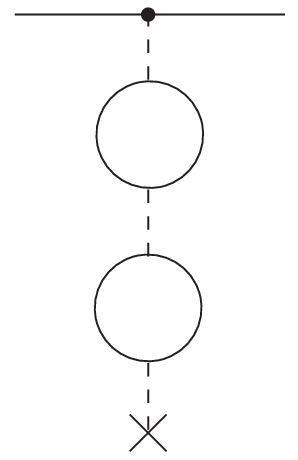
Figure 3: The second-order Uehling contributions to the energy.

It is important that Eq. (1) includes only the first derivative with respect to $\kappa$ . That is because a shift in the effective mass is at most ${\cal O}((Z\alpha)^{2}(m/M)m)$ and terms quadratic in the shift are at most of the order $\varepsilon(Z\alpha)^{6}(m/M)^{2}m$ . To evaluate the derivative we apply the identity

\frac{\partial\left(f_{CN}({Z\alpha},\kappa)-1\right)^{2}}{\partial\ln\kappa}=-\frac{\partial\left(f_{CN}({Z\alpha},Z\alpha m_{R}/m_{e})-1\right)^{2}}{\partial\ln m_{e}}\;,

which allows us to avoid differentiating the $\alpha^{2}$ term in $f_{CN}({Z\alpha},Z\alpha m_{R}/m_{e})$ , found by means of numerical computation, and instead allows to calculate numerically an integral, which contains a derivative of the potential over the parameter $m_{e}$ .

The result for the Dirac equation with the reduced mass and the potential defined in Eq. (3) can be in principle obtained by many means. Recently such a result for low-lying states in light muonic atoms was found by applying a nonrelativistic perturbation theory in [6].

II eVP relativistic recoil corrections to the second order of $\alpha$

Let us expand Eq. (2) in terms of $\varepsilon$ :

	$\displaystyle f_{CN}({Z\alpha},Z\alpha m_{R}/m_{e})$	$\displaystyle=$	$\displaystyle f_{C}({Z\alpha})+f_{N}({Z\alpha},Z\alpha m_{R}/m_{e})$		(7)
			$\displaystyle+f_{NN}({Z\alpha},Z\alpha m_{R}/m_{e})\;,$		(7)

where $f_{N}$ is linear in $\varepsilon$ and $f_{NN}$ is quadratic.

It is convenient to consider different parts of the perturbing potential independently, setting appropriate $\varepsilon$ in different cases.

II.1 The first-order contribution of $V_{11}$ and $V_{2}$

To take into account the contributions of $V_{11}$ and $V_{2}$ , we can set $\varepsilon=(\alpha/\pi)^{2}$ and take the first order of the perturbation theory (in $\varepsilon$ ), which has been already studied in Ref. [5]¹¹ 1 To simplify notation we drop the arguments in terms of Eq. (1).

E_{Nq}^{(1)}=m_{R}f_{Nq}+\Delta E_{q}^{(1)}\,,

(8)

where the index $q$ corresponds to either $V_{11}$ or $V_{2}$ ,

$\displaystyle\Delta E_{q}^{(1)}$	$\displaystyle=$	$\displaystyle-\frac{m_{R}^{2}}{M}\Bigl(f_{C}-1\Bigr)f_{Nq}$	(9)
	$\displaystyle-$	$\displaystyle\frac{m^{2}_{R}}{M}(f_{C}-1)\frac{\partial}{\partial\ln\kappa}f_{Nq}$
	$\displaystyle-$	$\displaystyle\langle\psi_{C}\|\Bigl(\frac{V_{q}V_{C}}{M}+\frac{1}{4M}[V_{C},[\mathbf{p}^{2},W_{q}]]$
		$\displaystyle~~+\frac{1}{4M}[V_{q},[\mathbf{p}^{2},W_{C}]]\Bigr)\|\psi_{C}\rangle\,,$

$|\psi_{C}\rangle$ is the Coulomb wave function and it is sufficient to consider it in the nonrelativistic (NR) approximation (cf. [5]). The related auxiliary potential takes the form (cf. (10) of [5])

	$\displaystyle W_{q}({\mathbf{k}})$	$\displaystyle=$	$\displaystyle 8\pi(Z\alpha)\int_{0}^{1}dv\,\frac{\rho_{q}(v)}{({\mathbf{k}}^{2}+\lambda^{2})^{2}}\,,$
	$\displaystyle W_{q}(r)$	$\displaystyle=$	$\displaystyle{(Z\alpha)}\int_{0}^{1}dv\,\rho_{q}(v)\frac{e^{-\lambda r}}{\lambda}\,.$		(10)

Proceeding in the same way as in [5] (cf. Eq. (32) there), we obtain for these contributions (cf. [12, 13])

$\displaystyle\Delta E_{Nq}^{\rm(NR)}$	$\displaystyle=$	$\displaystyle\frac{(Z\alpha)^{4}}{n^{3}}\frac{m_{R}^{2}}{M}\sum_{i,k=0}^{n-l-1}B_{ik}^{\rm(NR)}$	(11)
	$\displaystyle\times$	$\displaystyle\Biggl[-\frac{1}{2n}K^{(q)}_{2,2l+i+k+2}(\kappa_{n})$
		$\displaystyle\phantom{9}-\frac{2l+i+k+2}{2n\kappa_{n}}K^{(q)}_{3,2l+i+k+3}(\kappa_{n})$
		$\displaystyle\phantom{9}+\frac{1}{\kappa_{n}}K^{(q)}_{3,2l+i+k+2}(\kappa_{n})\Biggr]\,,$

where

	$\displaystyle B_{ik}^{\rm(NR)}$	$\displaystyle=$	$\displaystyle\frac{(-1)^{i+k}(n-l-1)!}{i!(n-l-i-1)!k!(n-l-k-1)!}$		(12)
		$\displaystyle\times$	$\displaystyle\frac{(n+l)!(2l+i+k+1)!}{(2l+i+1)!(2l+k+1)!}$		(12)

and functions

\displaystyle K^{(q)}_{bc}(\kappa)

\displaystyle=

\displaystyle\int_{0}^{1}{dv}\,\frac{\rho_{q}(v)}{(1-v^{2})^{b/2-1}}\,\left(\frac{\kappa\sqrt{1-v^{2}}}{1+\kappa\sqrt{1-v^{2}}}\right)^{c}

(13)

differ from the base integrals $K_{bc}(\kappa)$ [12, 13], introduced earlier and expressed in terms of spectral functions.

For the low-lying states of interest ( $n=1,2$ ) in light muonic atoms the results are

$\displaystyle\Delta E_{q}^{\rm(NR)}(1s)$	$\displaystyle=$	$\displaystyle(Z\alpha)^{4}\,\frac{m_{R}^{2}}{M}\,$
	$\displaystyle\times$	$\displaystyle\frac{1}{\kappa}\biggl[-\frac{\kappa}{2}K^{(q)}_{22}(\kappa)+K^{(q)}_{32}(\kappa)-K^{(q)}_{33}(\kappa)\biggr]\;,$
$\displaystyle\Delta E_{q}^{\rm(NR)}(2s)$	$\displaystyle=$	$\displaystyle(Z\alpha)^{4}\,\frac{m_{R}^{2}}{32M}$
	$\displaystyle\times$	$\displaystyle\Biggl\{-K^{(q)}_{24}(\kappa_{2})+\frac{4}{\kappa_{2}}\Bigl[K^{(q)}_{34}(\kappa_{2})-K^{(q)}_{35}(\kappa_{2})\Bigr]$
	$\displaystyle+$	$\displaystyle\frac{2}{\kappa_{2}^{3}}\Bigl[\kappa_{2}K^{(q)}_{44}(\kappa_{2})+4K^{(q)}_{54}(\kappa_{2})$
		$\displaystyle-4K^{(q)}_{55}(\kappa_{2})\Bigr]\Biggr\}\;,$
$\displaystyle\Delta E_{q}^{\rm(NR)}(2p)$	$\displaystyle=$	$\displaystyle(Z\alpha)^{4}\,\frac{m_{R}^{2}}{M}\,$	(14)
	$\displaystyle\times$	$\displaystyle\frac{1}{\kappa_{2}}\biggl[-\frac{\kappa_{2}}{2}K^{(q)}_{2,4}(\kappa_{2})+2K^{(q)}_{3,4}(\kappa_{2})$
		$\displaystyle-2K^{(q)}_{3,5}(\kappa_{2})\biggr]\,.$

The required integrals $K^{(11)}_{bc}$ and $K^{(2)}_{bc}$ should be calculated numerically. The numerical results are considered in Sec. III.

II.2 The second-order contribution of $V_{U}$

To deal with the second order contributions of $V_{U}$ (see, e.g, Fig. 3) we should address terms in (1) which are the second order in $\varepsilon=\alpha/\pi$ .

For the case of general $V_{N}$ , selecting terms of the corresponding order $\varepsilon^{2}$ in Eq. (1), we arrive at

E^{(2)}_{N}=m_{R}f_{NN}+\Delta E^{(2a)}_{N}+\Delta E^{(2b)}_{N}\,,

(15)

where

	$\displaystyle\Delta E^{(2a)}_{N}=-\frac{m_{R}^{2}}{M}\left(\vphantom{\frac{0}{0}}(f_{C}-1)f_{NN}+\frac{\bigl(f_{N}\bigr)^{2}}{2}\right)$
	$\displaystyle-\frac{m_{R}^{2}}{M}\left((f_{C}-1)\frac{\partial}{\partial\ln\kappa}f_{NN}+f_{N}\frac{\partial}{\partial\ln\kappa}f_{N}\right)\;.$		(16)

Note that in the last expression we need only the leading nonrelativistic contribution to various $f$ , and in particular it is sufficient to write

f_{NN}=\frac{\langle\psi_{C}|V_{N}G^{\prime}_{C}V_{N}|\psi_{C}\rangle}{m_{R}}\;,

(17)

where $G^{\prime}_{C}$ is the reduced Coulomb wave function for the corresponding state.

The second term in (15), $\Delta E^{(2b)}$ , corresponds to the $W$ contribution of the matrix element in (1), which in the second order of $\varepsilon$ provides us with

$\displaystyle\Delta E^{(2b)}_{N}$	$\displaystyle=$	$\displaystyle-\langle\psi_{C}\|\left(\frac{V_{N}^{2}}{2M}+\frac{1}{4M}[V_{N},[\mathbf{p}^{2},W_{N}]]\right)\|\psi_{C}\rangle$	(18)
	$\displaystyle-$	$\displaystyle 2\langle\psi_{C}\|\left(\frac{V_{C}V_{N}}{M}+\frac{1}{4M}[V_{N},[\mathbf{p}^{2},W_{C}]]\right.$
	$\displaystyle+$	$\displaystyle\left.\frac{1}{4M}[V_{C},[\mathbf{p}^{2},W_{N}]]\right)\|\psi_{N}\rangle\,,$

where

|\psi_{N}\rangle=G^{\prime}_{C}V_{N}|\psi_{C}\rangle

(19)

is the correction to the wave function induced by $V_{N}$ .

To calculate the correction to the second order in the Uehling potential we set $V_{N}=V_{U}$ in general expressions (16)–(19).

Equation (15) presents the complete result for the relativistic terms of order $\alpha^{2}(Z\alpha)^{4}m$ and $\alpha^{2}(Z\alpha)^{4}m^{2}/M$ in terms of the sum of the Dirac term with the reduced mass $m_{R}f_{NN}$ and the recoil corrections $\Delta E^{(2a)}_{U}$ and $\Delta E^{(2b)}_{U}$ . Since the expressions for the corrections deal with nonrelativistic wave functions and Green functions, the result for the eVP relativistic recoil correction depends on orbital momentum $l$ and does not depend on total muon angular momentum $j$ , which means that there is no corrections to the fine splitting in this order behind the result of the Dirac equation with the reduced mass.

III Results

The expressions presented above allow us to calculate the recoil correction to the energy of order $(\alpha/\pi)^{2}(Z\alpha)^{4}m_{R}^{2}/M$ . The contributions to the correction for the lowest states of the muonic hydrogen

\Delta E^{\rm(rec-VP2)}=\Delta E^{(1)}_{11}+\Delta E^{(1)}_{2}+\Delta E^{(2a)}_{U}+\Delta E^{(2b)}_{U}

(20)

are listed for muonic hydrogen in Table 1.

	$1s$	$2s$	$2p$
$\Delta E^{(1)}_{11}$	$\phantom{-}0.505$	$\phantom{-}0.0721$	$\phantom{-}0.000133$
$\Delta E^{(1)}_{2}$	$\phantom{-}0.139$	$\phantom{-}0.0576$	$\phantom{-}0.002879$
$\Delta E^{(2a)}_{U}$	$-0.154$	$-0.0024$	$-0.000060$
$\Delta E^{(2b)}_{U}$	$\phantom{-}0.678$	$\phantom{-}0.0685$	$\phantom{-}0.000367$
$\Delta E^{\rm(rec-VP2)}$	$\phantom{-}1.168$	$\phantom{-}0.1958$	$\phantom{-}0.003319$

Table 1: The

\alpha^{2}

eVP relativistic recoil corrections to energies of the muonic hydrogen in units of

(\alpha/\pi)^{2}(Z\alpha)^{4}m_{R}^{2}/M

. See Eq. (20) for notation.

The first order Källen-Sabry potential contributions are calculated numerically in a rather straightforward way. To control the calculation of the irreducible part we have also used various approximate representations for the dispersion function. They are discussed in Appendix A.

The corrections of the second order in the Uehling potential were computed using two different representations of the reduced nonrelativistic Coulomb Green functions, which are summarized in Appendix B. The results produced with two representations are consistent.

The calculations were also performed for various isotopes of muonic hydrogen and helium ion. The results are presented in Table 2.

	$1s$	$2s$	$2p$
H	$1.168$	$0.1958$	$0.003319$
D	$1.192$	$0.2016$	$0.003551$
³He⁺	$1.445$	$0.2867$	$0.006866$
⁴He⁺	$1.447$	$0.2878$	$0.006900$

Table 2: The

\alpha^{2}

relativistic recoil eVP corrections to energies of the light muonic hydrogen-like atoms in units

(\alpha/\pi)^{2}(Z\alpha)^{4}m_{R}^{2}/M

It is interesting to compare results obtained with the Grotch-type calculations in this paper with the Breit-type calculation we perform previously [6].

A comparison of the Grotch-type results with the complete Breit-type ones is summarized in Table 3. The Breit-type results are exact in $m/M$ , while the Grotch-type recoil correction includes only a term linear in $m/M$ . As explained in [5, 6] (see also [14]), one can rearrange the Breit Hamiltonian and separate the linear recoil and higher-order terms. As stated in [6], the linear recoil terms in the Breit-type approach are consistent with the results obtained here; in fact they agree within an uncertainty of numerical integration and, therefore, all digits in the results given for the Grotch-type evaluation in Table 3 are valid.

Atom	$~~1s$	$~~2s$	$~~~2p_{1/2}$	$~~~2p_{3/2}$
H	0.172	0.0288	0.000488	0.000488
	0.155	0.0259	0.000737	0.000289
D	0.0973	0.0165	0.000290	0.000290
	0.0921	0.0156	0.000370	0.000227
³He⁺	1.31	0.259	0.00621	0.00621
	1.26	0.250	0.00810	0.00492
⁴He⁺	1.00	0.200	0.00478	0.00478
	0.97	0.194	0.00590	0.00403

Table 3: The

\alpha^{2}

relativistic recoil eVP corrections to energies of light muonic hydrogen-like atoms in units of

\mu

eV. The eVP2 results of the Grotch-type evaluation of this paper are given in roman type. The complete results of the Breit-type calculations [6] are presented in italics. Note that the complete Breit-type recoil results [6] of order

\alpha^{2}(Z\alpha)^{4}m

are exact in

m/M

, while the Grotch-type recoil contributions include only terms linear in

m_{R}/M

As one can see from Table 3, the higher-order terms in $m/M$ are important for the complete recoil results. For the $s$ states in muonic hydrogen they are about 10% of the linear term. (Here in Table 3 the Darwin-Foldy-type terms are included for all atoms. If, following [15, 16], we exclude them, the results are shifted and become 0.0635 $\mu$ eV ( $1s$ ), 0.0126 $\mu$ eV ( $2s$ ) for muonic deuterium and 0.75 $\mu$ eV ( $1s$ ), 0.172 $\mu$ eV ( $2s$ ) for muonic helium-4). For the $p$ states the $(m/M)^{2}$ contribution is even larger in fractional units, however, the total recoil contribution for the $2p$ state is small in comparison with the related $2s$ contribution and can be neglected for the $2p-2s$ difference, while calculating the Lamb shift. A similar situation actually also takes place for the one-loop eVP contribution [14, 5].

The Breit-type calculations [6] delivered all the contributions within a nonrelativistic perturbation theory (NRPT) with various relativistic perturbations of the Coulomb potential.

Within the Breit-equation approach, the recoil and non-recoil terms of the Breit Hamiltonian are treated in the same way (see, e.g., [2]). As a result, the technique applied in [6] to obtain the relativistic non-recoil term (i.e. the relativistic correction to the one-particle equation with the reduced mass) was the same as for the recoil term. Actually, within the NRPT approach there is no need for a separation between the recoil and non-recoil terms.

Here, the recoil correction is obtained in a quite different way. Thus, we conclude that our NRPT calculation of both the non-recoil and recoil relativistic contributions [6] is correct.

To conclude, the results of this paper include the development of a method to calculate the second-order-eVP relativistic recoil correction for an arbitrary state in an arbitrary hydrogen-like muonic atom. That is a purely theoretical result. As for an application to practically important transitions, we have calculated the relativistic recoil correction of order $\alpha^{2}(Z\alpha)^{4}m^{2}/M$ for the Lamb shift in muonic hydrogen. It is small by itself. As we explain above, such a calculation serves as a confirmation of our eVP results previously obtained by means of NRPT [6]. Because of the way relativistic recoil and non-recoil contributions were treated there, the result of this paper confirms the whole relativistic eVP contribution of [6] and in particular its relativistic non-recoil correction of order $\alpha^{2}(Z\alpha)^{4}m$ . That correction, in contrast to the recoil term, is somewhat smaller than, but still compatible with the uncertainty of actual experiments (see [6] for details).

Acknowledgments

This work was supported in part by DFG under Grant No. GZ: HA 1457/7-2 and RFBR under Grant No. 12-02-31741. Part of the work was done while V.G.I. and E.Y.K. stayed at the Max-Planck-Institut für Quantenoptik, and they are grateful for the warm hospitality they received.

Appendix A Approximation for the irreducible part of the Källen-Sabry dispersion function with an uncertainty better than 1%

The exact expression for the irreducible part of the dispersion weight function of the Källen-Sabry potential [7, 8, 9]

$\displaystyle\rho_{2}(v)$	$\displaystyle=$	$\displaystyle\frac{2}{3}\left(\frac{\alpha}{\pi}\right)^{2}\frac{v}{1-v^{2}}\times\biggl\{(3-v^{2})(1+v^{2})$	(21)
		$\displaystyle\left[{\rm Li}_{2}\left(-\frac{1-v}{1+v}\right)+2{\rm Li}_{2}\left(\frac{1-v}{1+v}\right)\right.$
	$\displaystyle+$	$\displaystyle\left.\ln\left(\frac{1+v}{1-v}\right)\left(\frac{3}{2}\ln\left(\frac{1+v}{2}\right)-\ln\left(v\right)\right)\right]$
	$\displaystyle+$	$\displaystyle\left(\frac{11}{16}(3-v^{2})(1+v^{2})+\frac{1}{4}v^{4}\right)\ln\left(\frac{1+v}{1-v}\right)$
	$\displaystyle+$	$\displaystyle\frac{3}{2}v(3-v^{2})\ln\left(\frac{1-v^{2}}{4}\right)-2v(3-v^{2})\ln(v)$
	$\displaystyle+$	$\displaystyle\frac{3}{8}v(5-3v^{2})\biggr\}$

is somewhat complicated. It does not allow us exact analytic evaluations in muonic atoms. Meanwhile an approximate representation by Schwinger [7]

\rho^{\rm(s)}_{2}(v)=\left(\frac{\alpha}{\pi}\right)^{2}\frac{v^{2}(1-\frac{v^{2}}{3})}{1-v^{2}}\left\{\frac{\pi^{2}}{2v}-\frac{3+v}{4}\left(\frac{\pi^{2}}{2}-\frac{3}{4}\right)\right\}

(22)

is a well-known successful approximation. It allows us to find contributions of the irreducible two-loop vacuum polarization to various values with a high accuracy. Since it reproduces the correct behavior of the dispersion density at $v\simeq 0$ (i.e., for $s\simeq s_{\rm threashold}$ ) and $v\simeq 1$ (i.e.. for $s\to\infty$ ), it may be considered as an extrapolation formula. Because of that it is useful not only to approximately find various numeric contributions, but also to approximate certain asymptotics.

Here, we present a few more extrapolations which in certain respects are more accurate than Schwinger’s [7]. They are

$\displaystyle\rho^{(1)}_{2}(v)$	$\displaystyle=$	$\displaystyle\left(\frac{\alpha}{\pi}\right)^{2}\frac{v}{1-v^{2}}$	(23)
	$\displaystyle\times$	$\displaystyle\biggl\{\frac{1}{2}v^{2}+(1-v^{2})\left(\frac{\pi^{2}}{2}-2.62\,v\right)\biggr\}\;,$	(23)
$\displaystyle\rho^{(2)}_{2}(v)$	$\displaystyle=$	$\displaystyle\left(\frac{\alpha}{\pi}\right)^{2}\frac{v}{1-v^{2}}$	(24)
		$\displaystyle\times\biggl\{\left(\frac{1}{2}+0.288(1-v^{2})\right)v^{2}$
		$\displaystyle+(1-v^{3})\left(\frac{\pi^{2}}{2}-3.695\,v\right)\biggr\}\;,$
$\displaystyle\rho^{(3)}_{2}(v)$	$\displaystyle=$	$\displaystyle\left(\frac{\alpha}{\pi}\right)^{2}\frac{v}{1-v^{2}}$	(25)
		$\displaystyle\times\biggl\{\left(\frac{1}{2}+1.08(1-v^{2})\right)v^{2}$
		$\displaystyle+(1-v^{3})\left(\frac{\pi^{2}}{2}-3.97\,v-0.28\,v^{3}\right)\biggr\}\;.$

The quality of these approximations can be discussed in the following way. We note that the density function is always positive. If we are to calculate a matrix element which does not change sign, such as an average of the irreducible part of the Källen-Sabry potential over a certain state, then the fractional error cannot exceed the maximal fractional error of the approximation of $\rho_{2}(v)$ in (21) by an approximate function. In general, if there are not specific cancelations, the fractional error determines the fractional uncertainty of any integrals.

Such an error

\delta^{\rm approx}(v)=\frac{\rho^{\rm approx}_{2}(v)-\rho_{2}(v)}{\rho_{2}(v)}

is plotted for the considered approximations in Fig. 4 along with the Schwinger approximation. The maximal values $\delta^{\rm max}$ of the fractional deviation are collected in Table 4.

Approximation	$\delta^{\rm max}$
$\rho^{\rm(s)}_{2}(v)$	4%
$\rho^{(1)}_{2}(v)$	2%
$\rho^{(2)}_{2}(v)$	0.55%
$\rho^{(3)}_{2}(v)$	0.3%

Table 4: The maximal values

\delta^{\rm max}

of the fractional deviation

\delta^{\rm approx}(v)

for various approximations.

We note that the accuracy of polynomial approximations for the expression in the large parentheses in Eq. (A1) is limited

We note that the accuracy of polynomial approximation for the expression in curly brackets in Eq. (21) is limited. It is clear that the behavior close to $v=0$ and $v=1$ should include logarithmic factors $\ln(v)$ and $\ln(1-v)$ , respectively. Those cannot be approximated with polynomials. However, approximations of $\rho_{2}(v)$ with uncertainty below 1% are possible.

The application of the approximate formulas to the calculation of the relativistic and relativistic recoil corrections is summarized in Tables 5 and 6. The fractional errors do not exceed the values of $\delta^{\rm max}$ collected in Table 4.

$\rho_{2}(v)$	$1s_{1/2}$	$2s_{1/2}$	$2p_{1/2}$	$2p_{3/2}$
Axact $\rho_{2}(v)$	$-0.5856$	$-0.1026$	$-0.03110$	$-0.003754$
$\rho^{\rm(s)}_{2}(v)$	$-0.5909$	$-0.1035$	$-0.03124$	$-0.003763$
$\rho^{(1)}_{2}(v)$	$-0.5844$	$-0.1024$	$-0.03100$	$-0.003754$
$\rho^{(2)}_{2}(v)$	$-0.5861$	$-0.1027$	$-0.03114$	$-0.003759$
$\rho^{(3)}_{2}(v)$	$-0.5859$	$-0.1027$	$-0.03112$	$-0.003756$

Table 5: The relativistic contribution to the energies for the irreducible part of the Källen-Sabry potential in muonic hydrogen. Units are

(\alpha/\pi)^{2}(Z\alpha)^{4}m_{R}

. The numerical results are for the solution of the Dirac equation with the reduced mass.

$\rho_{2}(v)$	$1s$	$2s$	$2p$
Exact $\rho_{2}(v)$	$0.1390$	$0.05762$	$0.002879$
$\rho^{\rm(s)}_{2}(v)$	$0.1425$	$0.05837$	$0.002895$
$\rho^{(1)}_{2}(v)$	$0.1401$	$0.05765$	$0.002868$
$\rho^{(2)}_{2}(v)$	$0.1392$	$0.05767$	$0.002881$
$\rho^{(3)}_{2}(v)$	$0.1391$	$0.05765$	$0.002880$

Table 6: The relativistic recoil contribution to the energies

\Delta E^{(1)}_{2}

for the irreducible part of the Källen-Sabry potential in muonic hydrogen in units of

(\alpha/\pi)^{2}(Z\alpha)^{4}m_{R}^{2}/M

The application of the approximations could be useful not only for tests but also for approximate analytic expressions (cf. [17, 12, 13, 18]).

Appendix B Representation of the reduced nonrelativistic Coulomb Green function in coordinate space

The nonrelativistic Coulomb Green’s function

G_{E}({\bf r},{\bf r}^{\prime})=\sum\frac{|\lambda\rangle\langle\lambda|}{E-E_{\lambda}}

and its reduced form

G^{\prime}_{E,nlm}({\bf r},{\bf r}^{\prime})={\sum}^{\prime}\frac{|\lambda\rangle\langle\lambda|}{E-E_{\lambda}}\;,

where one has to sum over all intermediate states $\lambda$ for $G_{E}$ and for all but the reference state $nlm$ for the reduced one, have a number of useful representations.

It is helpful to separate the radial and angular parts for the partial contributions in the full Green’s function

	$\displaystyle G_{E}({\bf r},{\bf r}^{\prime})$	$\displaystyle=$	$\displaystyle\sum_{lm}\,{G}_{E,nl}(r,r^{\prime})\,Y_{lm}^{\star}(\Omega)Y_{lm}(\Omega^{\prime})$		(26)
		$\displaystyle=$	$\displaystyle\frac{2l+1}{4\pi}\,{G}_{E,nl}(r,r^{\prime})\,P_{l}(\cos\theta)\,,$		(26)

where $Y_{lm}(\Omega)$ are spherical harmonics, $m$ is the projection of orbital momentum, $\Omega$ is the angular variable, $P_{l}(\cos\theta)$ is the Legendre polynomial and $\theta$ is the angle between ${\bf r}$ and ${\bf r}^{\prime}$ . A similar separation can be also done for the reduced Green functions.

In our calculations we deal with matrix elements as

\langle nlm|AG^{\prime}_{E_{nlm},nlm}B|nlm\rangle\;,

where $A$ and $B$ are for central potentials. In such a case the only partial contribution surviving in the sum over $lm$ in (26) is ${G}_{E,nlm}$ . The result for the matrix element does not depend on $m$ . For further consideration we denote it as ${G}_{E,nl}$ . For the reduced Green function with $E=E_{nl}$ , we denote the surviving term in the partial sum as $G^{\prime}_{nl}$ .

In our paper we apply two representations, which are described below.

B.1 The Hostler presentation

One of the efficient representations of the nonrelativistic Coulomb Green function was derived by Hostler [19]

	$\displaystyle G_{E,nl}({\bf r},{\bf r}^{\prime})$	$\displaystyle=$	$\displaystyle\frac{4Z\alpha\,m_{r}^{2}}{\nu\,z_{>}z_{<}}\frac{\Gamma(1+l-\nu)}{\Gamma(2l+2)}\,$		(27)
		$\displaystyle\times$	$\displaystyle W_{\nu,l+1/2}(z_{>})M_{\nu,l+1/2}(z_{<})\,,$		(27)

where

$\displaystyle\nu$	$\displaystyle=$	$\displaystyle\frac{Z\alpha\,m_{r}}{\sqrt{-2m_{r}E}}\,,$	(28)
$\displaystyle z_{>}$	$\displaystyle=$	$\displaystyle\frac{2Z\alpha\,m_{r}}{\nu}{\rm max}(r,r^{\prime})\,,$	(29)
$\displaystyle z_{<}$	$\displaystyle=$	$\displaystyle\frac{2Z\alpha\,m_{r}}{\nu}{\rm min}(r,r^{\prime})\,,$	(30)

$\Gamma(x)$ is the Gamma function, and $M_{\mu\nu}(x)$ and $W_{\mu\nu}(x)$ are the Whittaker functions [20].

The required radial parts of the reduced Coulomb Green’s functions of the states of interest are [21, 22, 23]

$\displaystyle{G}^{\prime}_{1s}(r,r^{\prime})$	$\displaystyle=$	$\displaystyle 4Z\alpha\,m_{r}^{2}\,\exp{\left(-\frac{z_{>}+z_{<}}{2}\right)}\biggl\{\frac{1}{z_{>}}+\frac{1}{z_{<}}$	(31)
		$\displaystyle+\frac{7}{2}-\frac{z_{>}+z_{<}}{2}+{\rm Ei}(z_{<})-2C$
		$\displaystyle-\ln(z_{>}z_{<})-\frac{e^{z_{<}}}{z_{<}}\biggr\}\,,$

$\displaystyle{G}^{\prime}_{2s}(r,r^{\prime})$	$\displaystyle=$	$\displaystyle Z\alpha\,m_{r}^{2}\frac{\exp\left(-\frac{z_{>}+z_{<}}{2}\right)}{4z_{>}z_{<}}\biggl\{8z_{<}-4z_{<}^{2}+8z_{>}$	(32)
	$\displaystyle+$	$\displaystyle 12z_{>}z_{<}-26z_{>}z_{<}^{2}+2z_{>}z_{<}^{3}-4z_{>}^{2}$
	$\displaystyle-$	$\displaystyle 26z_{>}^{2}z_{<}+23z_{>}^{2}z_{<}^{2}-z_{>}^{2}z_{<}^{3}+2z_{>}^{3}z_{<}$
	$\displaystyle-$	$\displaystyle z_{>}^{3}z_{<}^{2}+4(z_{>}-2)z_{>}(1-z_{<})e^{z_{<}}$
	$\displaystyle+$	$\displaystyle 4(z_{>}-2)z_{>}(z_{<}-2)z_{<}$
	$\displaystyle\times$	$\displaystyle\bigl[-2C+{\rm Ei}(z_{<})-\ln(z_{>}z_{<})\bigr]\biggr\}\,,$

$\displaystyle{G}^{\prime}_{2p}(r,r^{\prime})$	$\displaystyle=$	$\displaystyle Z\alpha\,m_{r}^{2}\frac{\exp\left(-\frac{z_{>}+z_{<}}{2}\right)}{36(z_{>}z_{<})^{2}}\biggl\{24z_{<}^{3}+36z_{>}z_{<}^{3}$	(33)
	$\displaystyle+$	$\displaystyle 36z_{>}^{2}z_{<}^{3}+24z_{>}^{3}+36z_{>}^{3}z_{<}+36z_{>}^{3}z_{<}^{2}$
	$\displaystyle+$	$\displaystyle 49z_{>}^{3}z_{<}^{3}-3z_{>}^{3}z_{<}^{4}-3z_{>}^{4}z_{<}^{3}$
	$\displaystyle-$	$\displaystyle 12z_{>}^{3}(2+z_{<}+z_{<}^{2})e^{z_{<}}+12z_{>}^{3}z_{<}^{3}$
	$\displaystyle\times$	$\displaystyle\bigl[-2C+{\rm Ei}(z_{<})-\ln(z_{>}z_{<})\bigr]\biggr\}\,,$

where $C=0.577\,216\ldots$ is the Euler constant, and

{\rm Ei}(x)=\int\limits_{-\infty}^{x}\frac{e^{t}}{t}dt

is the exponential integral.

B.2 The Sturmian representation

The Sturmian presentation of the nonrelativistic Coulomb Green’s function is a presentation in terms of a basis set which consists of solutions of the related Sturm-Liouville problem.

The basis functions satisfy the equation

{\bf p}^{2}\Phi_{klm}(\nu;\;{\bf r})=2m_{r}\left(\frac{k}{\nu}\,\frac{Z\alpha}{r}+E\right)\Phi_{klm}(\nu;\;{\bf r})\,,

(34)

where

\nu=\sqrt{-\frac{(Z\alpha)^{2}m}{2E}}\,.

They can be presented in the form

\Phi_{klm}(\nu;\;{\bf r})=R_{kl}(\nu;r)Y_{lm}(\Omega)\,,

where

R_{kl}(\nu;\;r)=\left(\frac{k}{\nu}\right)^{3/2}R_{kl}\left(\frac{k}{\nu}\,r\right)\;,

and $R_{kl}(r)$ stands for the radial part of the standard wave function of the nonrelativistic Coulomb problem (see, e.g., [24]).

The radial part of the Coulomb Green’s function is of the form [25]

G_{El}(r;r^{\prime})=\frac{\nu^{2}}{(Z\alpha)^{2}m}\sum_{k=l+1}^{\infty}\frac{k}{k-\nu}R_{kl}\left(\nu;\;r\right)R_{kl}\left(\nu;\;r^{\prime}\right)\,.

(35)

The required radial part of the reduced Coulomb Green’s function (at $E=E_{n}$ ) is of the form [25]

$\displaystyle{G}^{\prime}_{nl}(r,r^{\prime})$	$\displaystyle=$	$\displaystyle\frac{n^{2}}{(Z\alpha)^{2}m_{r}}\Biggl\{\sum_{k=l+1\atop k\neq n}^{\infty}\frac{k}{k-n}R_{kl}(n;r)R_{kl}(n;r^{\prime})$	(36)
	$\displaystyle+$	$\displaystyle\frac{3}{2}R_{nl}(n;r)R_{nl}(n;r^{\prime})$
	$\displaystyle+$	$\displaystyle rR^{\prime}_{nl}(n;r)R_{nl}(n;r^{\prime})$
	$\displaystyle+$	$\displaystyle r^{\prime}R^{\prime}_{nl}(n;r^{\prime})R_{nl}(n;r)\Biggr\}\,,$

where

R^{\prime}_{nl}(n;r)=\frac{\partial}{\partial r}R_{nl}(n;r)\;.

References

[2] V.B. Berestetskii, E.M. Lifshitz, and L.P. Pitaevskii, Quantum Electrodynamics, Pergamon Press, Oxford (1982).
[3] H. Grotch and D.R. Yennie, Z. Phys., 202, 425 (1967).
[4] S.G. Karshenboim, V.G. Ivanov, and E.Yu. Korzinin, Phys. Rev. A 89, 022102 (2014); arXiv:1311.5789.
[5] V.G. Ivanov, E.Yu. Korzinin, and S.G. Karshenboim, Phys. Rev. A 89, 022103 (2014); arXiv:1311.5790;
[6] E.Yu. Korzinin, V.G. Ivanov, and S.G. Karshenboim, Phys. Rev. D 88, 125019 (2013); arXiv:1311.5784.
[7] J. Schwinger. Particles, Sources, and Fields (Perseus, Reading, MA¡ 1998), Vol 2.
[8] G. Källen and A. Sabry, K. Dan. Vidensk. Selsk. Mat.-Fys. Medd., 29 (1955) No.17.
[9] M.I. Eides, S.G. Karshenboim, and V.A. Shelyuto, Phys. Lett., B 229, 285 (1989);
S.G. Karshenboim, V.A. Shelyuto, and M.I. Eides. Yad. Fiz. 50, 1636 (1989) [Sov. J. Nucl. Phys., 50, 1015 (1989)].
[10] S.G. Karshenboim, E.Yu. Korzinin, and V.G. Ivanov, JETP Letters 88, 641 (2008).
[11] L. Lewin. Dilogarithms and Associated Functions (Macdonald, London, 1958).
[12] S.G. Karshenboim, Can. J. Phys. 76, 169 (1998);
Zh. Eksp. Teor. Fiz. 116, 1575 (1999) [Sov. Phys. JETP 89, 850 (1999)].
[13] E.Yu. Korzinin, V.G. Ivanov, and S.G. Karshenboim, Eur. Phys. J. D 41, 1 (2007).
[14] S.G. Karshenboim, V.G. Ivanov, and E.Yu. Korzinin, Phys. Rev. A 85, 032509 (2012).
[15] D. A. Owen, Phys. Rev. D 42, 3534 (1990); D 46, 4782 (E) (1992).
[16] K. Pachucki and S. G. Karshenboim, J. Phys. B 28, L221 (1995).
[17] A.B. Mickelwait and H.C. Corben, Phys. Rev. 96, 1145 (1954);
G.E. Pustovalov, Zh. Eksp. Teor. Fiz. 32, 1519 (1957) [Sov. Phys. JETP 5, 1234 (1957)];
D.D. Ivanenko and G.E. Pustovalov. Usp. Fiz. Nauk 61, 27 (1957) [Adv. Phys. Sci. 61, 1943 (1957)].
[18] S.G. Karshenboim, V.G. Ivanov, and E.Yu. Korzinin, Eur. Phys. J. D 39, 351 (2006).
[19] L. Hostler, J. Math. Phys. 5, 591(1964).
[20] E. T. Whittaker, G. N. Watson (1996) A Course of Modern Analysis, 4th ed. (Cambridge University Press, Cambridge, 1996).
[21] H.F. Hameka, J. Chem. Phys. 47, 2728 (1967); Erratum. 48, 4810 (1968).
[22] L.C. Hostler, Phys. Rev. 178, 126131 (1969).
[23] K. Pachucki, Phys. Rev. A53, 2092 (1996).
[24] L.D. Landau, E.M. Lifshitz. Quantum Mechanics: Non-Relativistic Theory, 3rd ed. (Pergamon Press, Oxford, 1977), Vol. 3.
[25] P.P. Pavinsky and A.I. Sherstyuk, Vest. Len. Gos. Univ. 22, 11 (1968);
L. Hostler, J. Math. Phys. 11, 2966 (1970);
S.V. Khristenko and S.I. Vechnikin, Opt. Spektrosk. 31, 503 (1971);
S.A. Zapryagaev, N.L. Manakov, and L.P. Rapoport, Yad. Fiz. 15, 508 (1972) [Sov. J. Nucl. Phys. 15, 282 (1972)];
S.V. Khristenko, Teor. Mat. Fiz. 22 35 (1975) [Theor. and Math. Phys., 22 21 (1975)].

Relativistic recoil effects to energy levels in a muonic atom: a Grotch-type calculation of the second-order vacuum-polarization contributions

Abstract

pacs

I Introduction

II eVP relativistic recoil corrections to the second order of α\alpha

II.1 The first-order contribution of V11V_{11} and V2V_{2}

II.2 The second-order contribution of VUV_{U}

III Results

Acknowledgments

Appendix A Approximation for the irreducible part of the Källen-Sabry dispersion function with an uncertainty better than 1%

Appendix B Representation of the reduced nonrelativistic Coulomb Green function in coordinate space

B.1 The Hostler presentation

B.2 The Sturmian representation

References

II eVP relativistic recoil corrections to the second order of $\alpha$

II.1 The first-order contribution of $V_{11}$ and $V_{2}$

II.2 The second-order contribution of $V_{U}$