Circular geodesics of naked singularities in the Kehagias-Sfetsos metric of Hořava’s gravity
Abstract
We discuss photon and test-particle orbits in the Kehagias-Sfetsos (KS) metric. For any value of the Hořava parameter , there are values of the gravitational mass for which the metric describes a naked singularity, and this is always accompanied by a vacuum “antigravity sphere” on whose surface a test particle can remain at rest (in a zero angular momentum geodesic), and inside which no circular geodesics exist. The observational appearance of an accreting KS naked singularity in a binary system would be that of a quasi-static spherical fluid shell surrounded by an accretion disk, whose properties depend on the value of , but are always very different from accretion disks familiar from the Kerr-metric solutions. The properties of the corresponding circular orbits are qualitatively similar to those of the Reissner-Nordström naked singularities. When event horizons are present, the orbits outside the Kehagias-Sfetsos black hole are qualitatively similar to those of the Schwarzschild metric.
pacs
04.50.Kd, 04.70.Bw, 04.40.Dg, 95.10.EgI Introduction
Hořava [1] proposed a theory of gravity motivated by a need to include quantum effects in the low-mass limit. Its action allows a spherically symmetric, asymptotically flat solution, which has been found by Kehagias and Sfetsos [2] in a modified version of the theory that is compatible with Minkowski vacuum. The solution involves a parameter, , in addition to the gravitational mass, , and tends to the Schwarzschild solution in the limit of large values of the dimensionless parameter product .
Presumably, is a universal constant, if the solution found in [2] correctly describes gravity. However the properties of the solution depend also on . For large masses, , the Kehagias-Sfetsos solution has event horizons, i.e., it corresponds to a black hole [2]. The current observational (lower) limits on are not particularly stringent [3, 4, 5, 6], and they are all compatible with the existence of stellar-mass naked singularities.
In this paper we discuss the circular geodesics of the KS solution, basing our work on the KS metric [2], Eq. (2), in which the gravitating object is either a black hole or a naked singularity, depending on its gravitational mass (once the Hořava parameter, , is fixed at any value).
Circular time-like geodesics are, of course, of great astronomical interest, predating even the birth of physics. Currently they play a fundamental role not only in investigations of planetary motion, but also in the dynamics of galaxies and of the brightest X-ray sources, such as quasars and X-ray binaries, where the emissions are powered by accretion disks. The properties of accretion disks, such as their luminosity, photon spectrum, time variability and the possible presence of an inner edge of the disk close to the ISCO (innermost stable circular orbit) are all intimately related to the properties of circular orbits of the accreting fluid [7, 8, 9, 10, 11].
The astrophysical information is carried from the disk to the observer by photons travelling through the cosmic vacuum, so null geodesics are of great interest as well. Further, circular photon orbits, present already in the Schwarzschild solution to Einstein’s general relativity (GR), may leave behind an observable time signature [12, 13].
Testing GR and alternative theories of gravity provides an aditional motivation for the current study. Geodesics around KS black holes have already been studied in [14, 15, 16], as well as circular motion and accretion disks in slowly rotating extensions of the KS spacetime in [17]. For any value of , a sufficiently small value will allow the naked singularity KS solution. Differences in the properties of accretion disks around black holes and putative naked singularites have been discussed in a different, GR, context [18]. If the properties of the observed stellar mass black hole candidates turn out to be incompatible with the theoretical properties of the KS naked singularities, this will provide a stringent lower limit to the value of the Hořava parameter [19]. Accordingly, we focus on the orbital properties of the KS spacetime in the naked singularity case. Similar investigations were recently carried out for the Reissner-Nordström metric [20, 21], and a remarkable qualitative similarity between the properties of the circular geodesics of naked singularities in GR and in Hořava’s gravity is one of the conclusions of our paper.

II KS spacetime
The Kehagias-Sfetsos (KS) solution corresponds to a spherically symmetric, static metric
| (1) |
and has the form [2]:
| (2) |
with
| (3) |
The Schwarzschild solution is recovered in the limit of . Further insight into the properties of the metric may be gleaned from embedding diagrams [22].
At first sight there are two parameters in the metric coefficients, and . In fact, the KS metric depends on a single parameter alone, the combination . Indeed, in terms of ,
| (4) |
For convenience, we extend the domain to include , where we take . Note that and is continuous for all . The behavior of can be seen in Fig. 1, for different values of . As here, corresponds to the presence of an event horizon. This occurs [2] for , with two horizons present for all .
For the KS solution has an interesting feature, which distinguishes it from naked singularity solutions in GR: is finite everywhere. The metric coefficients are continuous at , with . However, their radial derivatives are not finite: as , and this leads to a singularity in the curvature [2].
The radial acceleration of a static time-like observer is given by
| (5) |
The general properties of the KS metric imply that this acceleration vanishes at a certain radius in the naked singularity case (). Indeed, since is continuous and , , it follows from the Rolle-Lagrange theorem that there will be a radius at which . Further, as , this radius corresponds to a minimum of (Fig. 1), and this is a stable equilibrium position of any test particle. This radius, , at which , could be termed the “antigravity radius”. Its value is
| (6) |
The angular momentum and frequency of geodesics also vanish at . Below this radius the radial acceleration of a static observer points inwards and therefore there are no circular time-like geodesics, this is the case of repulsive gravity (antigravity). Thus, circular geodesics exist only for , and there are also stable time-like geodesics corresponding to rest at .
III Equatorial geodesic motion
To fix the notation we begin with a brief review of circular motion in a spherically symmetric, static metric, with signature (+ – – – ). For geodesics we have the following constants of motion:
| (7) |
| (8) |
respectively, the energy and angular momentum of a test particle. From these conserved quantities we can construct the specific angular momentum, also conserved,
| (9) |
For circular equatorial geodesics (const, ), we may write the specific angular momentum in terms of its angular velocity :
| (10) |
where (e.g., [10])
| (11) |
and
| (12) |

III.1 Time-like circular geodesics
The radial dependence of time-like equatorial geodesic motion is described by the equation
| (13) |
where the effective potential is defined by
| (14) |
From we obtain the angular momentum of circular geodesics:
| (15) |
This formula was obtained in [23] by a direct analysis of the geodesic equations.
The second derivative of the effective potential is related to the stability of circular motion. Indeed, evaluated at the circular orbit is proportional to the radial epicyclic frequency and hence its sign determines whether or not the Rayleigh criterion is satisfied [10]. This can also be seen from the relation
| (16) |
valid in the equatorial plane circular orbits of any static, axially symmetric spacetime. For time-like circular geodesics, and satisfy a precise relation [23] , and hence and satisfy
| (17) |
Thus, for the sign of is the same as that of and of . As is well known, radial stability corresponds to , or equally to , while radial instability corresponds to , i.e. to . The term between brackets in Eq. (17) is recognized as the particle’s circular velocity measured by a local static observer, .
III.2 Null circular geodesics
The motion of photons in the equatorial plane is described by the equation
| (18) |
with the effective potential
| (19) |
The condition for a circular photon orbit is . Maxima of correspond to radially unstable photon orbits, whereas minima of correspond to stable photon orbits. From (11), (19), and (15) we see that in any static, axially symmetric spacetime as the radius of the circular time-like geodesic approaches that of the photon orbit.

IV Geodesic motion in KS spacetime
| (20) |
| (21) |
| (22) |
| (23) |
| (24) |

The allowed regions for circular time-like motion have qualitatively different properties, depending on the value of , as summarized in Fig. 4. This figure shows the antigravity radius (solid line), the marginally stable orbits (dotted lines) and the photon orbits (dot-dashed lines). We also show the different regions of stability for circular time-like geodesics: stable region (dark gray), unstable region (light gray) and “forbidden” regions where no circular geodesics are allowed (white). There are two such forbidden regions: one between the two photon orbits (at lower values of ) or between the outer horizon and the unstable photon orbit (at higher values of ), and one where static observers suffer an inward radial acceleration (either the region , at lower values of , or the one between the singularity and the inner horizon, at higher values of ). The behavior of is depicted in Fig. 3; note the correspondence of the curves with the stability regions presented in Fig. 4. Since the spacetime is spherically symmetric, all circular time-like geodesics are vertically stable.
The photon radii in KS spacetime are positive solutions of the equation
| (25) |
and the two photon orbits merge at
| (26) |
for . An interesting feature of photon orbits in the KS naked singularity spacetime is that the inner photon orbit is stable. This fact can be seen directly from the behavior of , Eq. (20), and it is illustrated in Fig. 2. Related to this fact is a potentially relevant astrophysical consequence: for values of which admit the stable photon orbit there is also an inner region of stable time-like circular geodesics, as depicted in Fig. 4. This region of stability (with respect to both radial and vertical perturbations) extends from to the inner photon radius.
The point on the - plane at which the stable and unstable circular photon orbits merge into the marginally stable photon orbit, Eq. (26), is also the termination point of the locus of the marginally stable time-like orbits, as can be seen in Fig. 4. For there are no photon orbits.
For , with , there are two marginally stable orbits among the time-like circular geodesics. The inner one, at radius could be termed the OSCO as for all satisfying there are stable circular orbits, while the outer one, at , present for all is the ISCO familiar from the Schwarzschild metric, as there are stable circular orbits for all . Thus, there are two regions of stability of circular test-particle motion for . The OSCO and ISCO coincide for . For all circular orbits are stable down to .
V The effective potential for test particles
In this section, we systematically discuss the behavior of for test-particle motion in terms of .

For the black-hole case () the situation is analogous to the Schwarzschild metric (Fig. 5). For sufficiently high values of angular momentum has a maximum at , corresponding to an unstable circular orbit, and a minimum at , corresponding to a stable circular orbit. At a certain critical value of angular momentum, , the two extrema merge at the radius of the marginally stable circular orbit. The unstable, marginally stable, and stable orbit radii satisfy . Hence, in this case the marginally stable orbit is an ISCO. For no circular orbits are possible.

If the spacetime admits two photon orbits, which correspond to the limit of test-particle orbits (see Figs. 2-4). This is indeed the situation for the first two extrema of (Fig. 6). As increases (without bounds), both the minimum and maximum values of increase (without bounds). The marginally stable orbit appears (at a radius larger than that of the unstable photon orbit) in the minimum of , at . Note that a stable circular orbit is always present between and the stable photon orbit, while the unstable circular orbit and the second (familiar) stable circular orbit (both at radii larger than that of the unstable photon orbit) only for values of .
We note that the behavior of for high angular momentum, as shown in Fig. 6, is not a particular feature of the KS naked-singularity solution, but instead a property of geodesic motion. If there is a local maximum of at for every high value of and if this sequence of radii has a bounded limit as , this limit will correspond to an unstable circular photon orbit. In the same way, if there is a local minimum of at for every high value of and if this sequence of radii has a bounded limit as , this limit will correspond to a stable circular photon orbit.
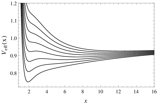

If we now consider there still are two separate regions of stability, but no photon orbit (Fig. 4). We see from Fig. 7 that the inner stable orbit is present for low values of , but as the magnitude of angular momentum is increased a marginally stable orbit is reached (the OSCO, see Fig. 3), and at higher values still of only the familiar outer stable orbits persist. Conversely, the outer stable orbits exist only for values of larger than the value in the ISCO. The unstable circular orbits exist only in a range of values, merging with the outer stable circular orbit at the lower end of the range (corresponding to the ISCO) and with the inner circular orbit at the higher end of the range (corresponding to the OSCO).
The last case is , for which the situation is analogous to ubiquitous motion in Newtonian gravity at . Fig. 8 shows that in this regime there is only one circular orbit for each value of angular momentum, and this orbit is stable. The orbits extend down to , which plays the role of the radius of a Newtonian star, or planet. However, it would be misleading to expect that the properties of the orbits as a function of their radius are the same as that of Keplerian orbits in a Newtonian potential, where the orbital frequency monotonically increases with . This cannot be the case here, as the angular frequency of the orbits goes to zero at both edges of the allowed domain, equally for and , implying that the (positive) angular frequency (squared) has a maximum. This is indeed the case, as can be seen in Fig. 9, which shows .

The profiles of the angular frequency , given by Eq. (24), in the three naked-singularity regimes defined by the values of are all similar. is always a curve with a zero at the gravity radius , it then monotonically increases, passes through a maximum—except for , when there is a region without circular orbits, so the domain of is not simply connected—and decreases monotonically tending to zero at infinity, for . For , a part of the curve corresponds to unstable orbits.
VI Discussion
The KS naked singularity in Hořava’s gravity has properties which distinguish it from those of the familiar Schwarzschild and Kerr solutions of GR. First, since at the singularity has the same value as at infinity, the singularity can be reached by a zero angular momentum test particle dropped from rest at infinity. However, if the particle loses some energy on its inbound trajectory, it will be reflected back and will oscillate between two turning points. If the energy loss continues, the particle will eventually settle at the minimum of the effective potential for radial motion of a test particle (Fig. 1), i.e., at the minimum of .
By the same token, since is finite in the neighbourhood of the singularity, being continuous, with (Eq. [4]), the effective potential for nonradial motion () will always present an infinite centrifugal barrier, so a particle carrying any angular momentum will never reach the singularity unless it manages to lose its angular momentum without losing energy. A more likely outcome is that the particle will lose both angular momentum and kinetic energy, in which case it also can settle at the minimum of . In view of spherical symmetry of the KS metric, this minimum has the form of the surface of a sphere. Inside this “antigravity sphere” static observers suffer an inward radial acceleration (an outward force).
We thus come to a most interesting conclusion. Accretion of matter by the naked KS singularity will result in accumulation of matter on the surface of a vacuum sphere around the naked singularity. Thus, an astrophysically relevant KS naked singularity will present the aspect of a spherical surface at the top of a shell of accumulated matter. For stellar-mass objects, the sphere will have a radius close to that of the gravitational radius of the naked singularity, .
If the naked singularity is in a binary system, it may accrete through a disk. It is thought that viscous dissipation in accretion disks is a result of MRI (the magnetorotational instability) [24], which occurs as long as angular frequency increases outwards, . As we can see in Fig. 9, this would occur only down to the maximum of . The maximum of is rather close to the naked singularity. Indeed, for within an order of magnitude or two of the black hole limit (), the maximum is at .
For the orbits are stable down to the antigravity radius (Figs. 4, 8, 9), so in this case we would have a quasistatic shell of fluid (accreted matter) on the surface of the hollow (vacuum) antigravity sphere concentric with the naked singularity, a cold, possibly opaque disk, abutting the sphere, and a hot accretion disk starting at a few gravitational radii. From the astronomical point of view, this system would present an aspect quite different from a Schwarzschild or Kerr black hole with an accretion disk with a hole in it (close to the ISCO) through which a second order lensed image of the disk can be observed. This suggests that a stringent constraint can be placed on the Hořava parameter through observation of astrophysical black holes ([19]).
VII Conclusions
We discussed photon and test-particle orbits in the Kehagias-Sfetsos metric as a function of the Hořava parameter times mass squared, . For naked singularities there are three different regimes of circular motion, depending on the value of . There is always an “antigravity sphere” on whose surface a test particle can remain at rest (in a zero angular momentum geodesic), and inside which no circular geodesics exist. For low values of the mass, circular motion is possible everywhere outside the antigravity sphere and is always stable. For intermediate mass values, there are two distinct regions of stable circular motion—the inner one terminates in an outer marginally stable circular orbit (OSCO) and the outer one begins in an inner marginally stable circular orbit (ISCO)—the two regions are separated by a region where circular orbits are unstable. For the largest values of compatible with the existence of a naked singularity there is an inner region of stable time-like circular geodesics, terminated by a stable photon orbit, and an outer region of stable circular geodesics beginning with an ISCO. Between the stable photon orbit and the ISCO there are two regions separated by an unstable circular photon orbit: in the inner one no circular orbits are allowed, and in the outer one circular time-like geodesics are unstable. The KS metric is static, and this is the only one we have considered. In GR it is known that the properties of orbits for rotating naked singularities differ from those of the static ones [25].
The properties of circular orbits of the Kehagias-Sfetsos and the Reissner-Nordström naked singularities are qualitatively similar (c.f., this work and [20, 21]), but very different from the black hole ones. When event horizons are present, the orbits outside the black hole are qualitatively similar to those of the Schwarzschild metric. No circular geodesics exist between the singularity and the inner horizon. The differences between the KS naked singularity and GR black hole cases may have astrophysical consequences, which we intend to explore in forthcoming papers. In particular, they may allow placing more stringent limits on the Hořava parameter ([19]).
Acknowledgements.
This work supported in part by Brazilian grant from “Fundação de Amparo à Pesquisa do Estado de São Paulo (FAPESP)”, no. 2013/01001-0, Czech grantCZ.1.07/2.3.00/20.0071 “Synergy” and Polish NCN grants UMO-2013/08/A/ST9/00795, UMO-2011/01/B/ST9/05439.References
- [1] P. Hořava, Phys. Rev. D 79, 084008 (2009).
- [2] A. Kehagias and K. Sfetsos, Phys. Lett. B 678, 123 (2011).
- [3] L. Iorio and M. L. Ruggiero, Int. J. Mod. Phys. A 25, 5399 (2010).
- [4] M. Liu, J. Lu, B. Yu, J. Lu, Gen. Rel. Grav. 43, 1401 (2011).
- [5] T. Harko, Z. Kovács and F. S. N. Lobo, Proc. R. Soc. A 467, 1390 (2011).
- [6] L. Iorio and M. L. Ruggiero, Int. J. Mod. Phys. D 20, 1079 (2011).
- [7] N. I. Shakura and R. A. Sunyaev, Astron. Astrophys. 24, 337 (1973).
- [8] I. D. Novikov and K.S. Thorne, in Black Holes, ed. C.DeWitt and B.S. DeWitt (New York: Gordon & Breach), p. 345 (1973).
- [9] W. Kluźniak, P. Michelson and R.V. Wagoner, Astrophys. J. 358, 538 (1990).
- [10] M. A. Abramowicz and W. Kluźniak, Astrophys. Sp. Sci. 300, 127 (2005).
- [11] A. Sa̧dowski, M. Abramowicz, M. Bursa, W. Kluźniak, J.-P. Lasota and A. Różańska, Astron. Astrophys. 527A, 17 (2011).
- [12] M. Bursa, M. A. Abramowicz, V. Karas and W. Kluźniak and A. Schwarzenberg-Czerny, RAGtime 8/9: Workshops on black holes and neutron stars, S. Hledík and Z. Stuchlík, eds, Silesian University in Opava (2007).
- [13] K. Fukumura, D. Kazanas and G. Stephenson, Astrophys. J. 695, 1199 (2009).
- [14] J. Chen and Y. Wang, Int. J. Mod. Phys. A 25, 1439 (2010).
- [15] A. Abdujabbarov, B. Ahmedov and A. Hakimov, Phys. Rev. D 83, 044053 (2011).
- [16] V. Enolskii, B. Hartmann, V. Kagramanova, J. Kunz, C. Lämmerzahl and P. Sirimachan, Phys. Rev. D 84, 084011 (2011).
- [17] T. Harko, Z. Kovács, and F. S. N. Lobo, Class. Quant. Grav. 28, 165001 (2011).
- [18] Z. Kovács and T. Harko, Phys. Rev. D 82, 124047 (2010).
- [19] M. A. Abramowicz, W. Kluźniak and R. S. S. Vieira, in preparation
- [20] Z. Stuchlík and S. Hledík, Acta Physica Slovaca 52, 363 (2002).
- [21] D. Pugliese, H. Quevedo and R. Ruffini, Phys. Rev. D 83, 024021 (2011).
- [22] K. Goluchová, K.Kulczycki, R. S. S. Vieira, Z. Stuchlìk, W. Kluźniak, M. Abramowicz, 2013, submitted.
- [23] P. S. Letelier, Phys. Rev. D 68, 104002 (2003).
- [24] S. A. Balbus and J. F. Hawley, Rev. Mod. Phys. 70, 1 (1998).
- [25] Z. Stuchlík, Astronomical Institutes of Czechoslovakia, Bulletin, 31, no. 3, p. 129-144 (1980).