跳到论文正文
W Papers独立论文阅读器 arXiv:1311.5648 论文正文 计算阅读时间 · 0%
引用这篇论文根据当前论文元数据生成,正式投稿前建议核对。


License: arXiv.org perpetual non-exclusive license
arXiv:1311.5648v3 [math.AT] 14 Feb 2014

Homological Stability For Moduli Spaces of Odd Dimensional Manifolds

Nathan Perlmutter Address: Department of Mathematics, University of Oregon, Eugene, OR, 97403, USA Email address: nperlmut@uoregon.edu
Abstract.

We prove a homological stability theorem for the moduli spaces of manifolds diffeomorphic to #g​(Sn+1×Sn)\#^{g}(S^{n+1}\times S^{n}), provided n≥4n\geq 4. This is an odd dimensional analogue of a recent homological stability result of S. Galatius and O. Randal-Williams for the moduli spaces of manifolds diffeomorphic to #g​(Sn×Sn)\#^{g}(S^{n}\times S^{n}) for n≥3n\geq 3.

1. Introduction

1.1. Main result

Recently S. Galatius and O. Randal-Williams proved a homological stability theorem for moduli spaces of certain manifolds of dimension 2​n2n where n≥3n\geq 3, see [4]. For a positive integer gg, denote by Vg,1V_{g,1} the connected sum #g​(Sn×Sn)−int(D2​n)\#^{g}(S^{n}\times S^{n})-\Int(D^{2n}) and by Diff(Vg,1)∂\Diff(V_{g,1})^{\partial} the topological group of diffeomorphisms of Vg,1V_{g,1} which fix a neighborhood of the boundary pointwise, equipped with the C∞C^{\infty}-topology. There is a natural map

sg:𝐁​Diff⁡(Vg,1)∂⟶𝐁​Diff⁡(Vg+1,1)∂s_{g}:\BDiff(V_{g,1})^{\partial}\longrightarrow\BDiff(V_{g+1,1})^{\partial}

induced by extending a diffeomorphism identically over an attached handle. S. Galatius and O. Randal-Williams proved that the map on homology induced by sgs_{g}

Hk​(𝐁​Diff⁡(Vg,1)∂,ℤ)⟶Hk​(𝐁​Diff⁡(Vg+1,1)∂,ℤ),H_{k}(\BDiff(V_{g,1})^{\partial};\mathbb{Z})\;\longrightarrow\;H_{k}(\BDiff(V_{g+1,1})^{\partial};\mathbb{Z}),

is an isomorphism provided that k≤12​(g−4)k\leq\frac{1}{2}(g-4), see [4, Theorem 1.2].

In this paper we prove an analogous result for diffeomorphism groups of similar odd-dimensional manifolds of dimension at least nine.

For a positive integer gg, denote by Wg,1W_{g,1} the (2​n+1)(2n+1)-dimensional manifold with boundary #g​(Sn+1×Sn)−int(D2​n+1)\#^{g}(S^{n+1}\times S^{n})-\Int(D^{2n+1}). Like with the case above, there is a natural map

(1) sg:𝐁​Diff⁡(Wg,1)∂⟶𝐁​Diff⁡(Wg+1,1)∂s_{g}:\BDiff(W_{g,1})^{\partial}\longrightarrow\BDiff(W_{g+1,1})^{\partial}

induced by extending a diffeomorphism identically over an attached copy of the cobordism W1,1−int(D2​n+1)W_{1,1}-\Int(D^{2n+1}). This map is defined rigorously in Section 2.1. We can now state our main theorem.

Theorem 1.1.

For n≥4n\geq 4 the map on homology induced by (1)

(sg)∗:Hk​(𝐁​Diff⁡(Wg,1)∂,ℤ)⟶Hk​(𝐁​Diff⁡(Wg+1,1)∂,ℤ),(s_{g})_{*}:H_{k}(\BDiff(W_{g,1})^{\partial};\mathbb{Z})\longrightarrow H_{k}(\BDiff(W_{g+1,1})^{\partial};\mathbb{Z}),

is an isomorphism provided that k≤12​(g−3)k\leq\frac{1}{2}(g-3).

1.2. Ideas behind the proof

Our methods are similar to those used in [4]. Namely, we construct a highly connected semi-simplicial space K∙​(Wg,1)K_{\bullet}(W_{g,1}) which admits a transitive action of the topological group Diff(Wg,1)∂\Diff(W_{g,1})^{\partial}. Roughly, the pp-simplices of K∙​(Wg,1)K_{\bullet}(W_{g,1}) are given by ordered lists of (p+1)(p+1)-many pair-wise disjoint embeddings of W1,1W_{1,1} into Wg,1W_{g,1} with a pre-prescribed boundary condition. This semi-simplicial space is almost identical to the one constructed in [4] and we use many of the same formal results from [4] regarding this semi-simplicial space. For instance, after proving that the geometric realization |K∙​(Wg,1)||K_{\bullet}(W_{g,1})| is highly connected, the proof of Theorem 1.1 goes through similarly to the proof of [4, Theorem 1.2].

However, in the proof of high-connectivity of |K∙​(Wg,1)||K_{\bullet}(W_{g,1})|, our methods differ from those of [4]. Our proof requires much of the theory regarding the diffeomorphism classification of highly connected manifolds developed by C.T.C. Wall in [10] and [11], specialized to the case of (n−1)(n-1)-connected, (2​n+1)(2n+1)-dimensional manifolds.

In more detail, let MM be an (n−1)(n-1)-connected, (2​n+1)(2n+1)-dimensional manifold. The homotopy groups πn​(Wg,1)\pi_{n}(W_{g,1}) and πn+1​(Wg,1)\pi_{n+1}(W_{g,1}) come equipped with the intersection parings

λn,n+1:πn​(M)×πn+1​(M)⟶πn​(Sn),λn+1,n+1:πn+1​(M)×πn+1​(M)⟶πn+1​(Sn),\begin{array}[]{c}\lambda_{n,n+1}:\pi_{n}(M)\times\pi_{n+1}(M)\longrightarrow\pi_{n}(S^{n}),\\ \\ \lambda_{n+1,n+1}:\pi_{n+1}(M)\times\pi_{n+1}(M)\longrightarrow\pi_{n+1}(S^{n}),\end{array}

and maps

αi:πi​(M)⟶πi−1​(S​O2​n+1−i)for i=n,n+1\alpha_{i}:\pi_{i}(M)\longrightarrow\pi_{i-1}(SO_{2n+1-i})\quad\quad\text{for \; $i=n,\;n+1$}

defined by sending a class x∈πi​(M)x\in\pi_{i}(M) to the class in πi−1​(S​O2​n+1−i)\pi_{i-1}(SO_{2n+1-i}) which classifies the normal bundle of an embedding which represents xx. (Indeed, for n≥4n\geq 4, the connectivity assumption on MM implies that all such elements x∈πi​(M)x\in\pi_{i}(M) for i=n,n+1i=n,n+1 are represented by embeddings, see [6]).

C.T.C. Wall shows that λn+1,n+1\lambda_{n+1,n+1} and αn+1\alpha_{n+1} are related by the summation formula,

αn+1​(a+b)=αn+1​(a)+αn+1​(b)+∂(λn+1,n+1​(a,b))for all a,b∈πn+1​(M)\alpha_{n+1}(a+b)\;=\;\alpha_{n+1}(a)\;+\;\alpha_{n+1}(b)\;+\;\partial(\lambda_{n+1,n+1}(a,b))\quad\text{for all $a,b\in\pi_{n+1}(M)$}

where ∂:πn+1​(Sn)→πn​(S​On)\partial:\pi_{n+1}(S^{n})\rightarrow\pi_{n}(SO_{n}) is the boundary map in the long-exact sequence associated to the fibre sequence, S​On→S​On+1→SnSO_{n}\rightarrow SO_{n+1}\rightarrow S^{n}, see [10].

For the case that M=Wg,1M=W_{g,1}, the map αn:πn​(Wg,1)→πn−1​(S​On+1)\alpha_{n}:\pi_{n}(W_{g,1})\rightarrow\pi_{n-1}(SO_{n+1}) is identically zero and the algebraic structure given by

(2) 𝕎g:=(πn​(Wg,1),πn+1​(Wg,1),λn,n+1,λn+1,n+1,αn+1){\mathbb{W}}_{g}:=(\pi_{n}(W_{g,1}),\;\pi_{n+1}(W_{g,1}),\;\lambda_{n,n+1},\;\lambda_{n+1,n+1},\;\alpha_{n+1})

has a particularly nice form. In this case we have isomorphisms

πn​(Wg,1)≅ℤ⊕g,andπn+1​(Wg,1)≅ℤ⊕g⊕(ℤ/2)⊕g.\pi_{n}(W_{g,1})\cong\mathbb{Z}^{\oplus g},\ \ \ \mbox{and}\ \ \ \pi_{n+1}(W_{g,1})\cong\mathbb{Z}^{\oplus g}\oplus(\mathbb{Z}/2)^{\oplus g}.

Furthermore, for the groups πn​(Wg,1)\pi_{n}(W_{g,1}) and πn+1​(Wg,1)\pi_{n+1}(W_{g,1}) there exist bases

(x1,…,xg)and(y1,…,yg,z1,…,zg),(x_{1},\dots,x_{g})\quad\text{and}\quad(y_{1},\dots,y_{g},z_{1},\dots,z_{g}),

with (z1,…,zg)(z_{1},\dots,z_{g}) a basis for the ℤ/2\mathbb{Z}/2-component of πn+1​(Wg,1)\pi_{n+1}(W_{g,1}), such that for i,j∈{1,…,g}i,j\in\{1,\dots,g\},

αn+1​(yi)=αn+1​(zi)=0,λn,n+1​(xi,yj)=δi,j⋅ιn,λn+1,n+1​(yi,zj)=δi,j⋅ρn+1,\alpha_{n+1}(y_{i})=\alpha_{n+1}(z_{i})=0,\quad\lambda_{n,n+1}(x_{i},y_{j})=\delta_{i,j}\cdot\iota_{n},\quad\lambda_{n+1,n+1}(y_{i},z_{j})=\delta_{i,j}\cdot\rho_{n+1},

where ιn∈πn​(Sn)\iota_{n}\in\pi_{n}(S^{n}) and ρn+1∈πn+1​(Sn)\rho_{n+1}\in\pi_{n+1}(S^{n}) are the standard generators. We call the algebraic structure given by the 55-tuple 𝕎g{\mathbb{W}}_{g} from (2) a Wall pairing of rank gg. In order to prove that the space |K∙​(Wg,1)||K_{\bullet}(W_{g,1})| is highly connected we study the action of Diff(Wg,1)∂\Diff(W_{g,1})^{\partial} on the Wall pairing 𝕎g{\mathbb{W}}_{g}.

We construct a simplicial complex Kπ​(Wg,1)K^{\pi}(W_{g,1}) whose pp-simplices are given by sets of (p+1)(p+1)-many pair-wise orthogonal (with respect to both λn,n+1\lambda_{n,n+1} and λn+1,n+1\lambda_{n+1,n+1}) embeddings 𝕎1↪𝕎g{\mathbb{W}}_{1}\hookrightarrow{\mathbb{W}}_{g} of the Wall pairings, mimicking embeddings of the manifolds W1,1↪Wg,1W_{1,1}\hookrightarrow W_{g,1}.

In this sense, the complex Kπ​(Wg,1)K^{\pi}(W_{g,1}) is an algebraic version of the semi-simplicial space K∙​(Wg,1)K_{\bullet}(W_{g,1}). In Section 5 we prove that the geometric realization |Kπ​(Wg,1)||K^{\pi}(W_{g,1})| is 12​(g−3)\frac{1}{2}(g-3)-connected. The connectivity of |Kπ​(Wg,1)||K^{\pi}(W_{g,1})| allows us to establish a lower bound for the connectivity of |K∙​(Wg,1)||K_{\bullet}(W_{g,1})|. At this point we use techniques developed by R. Charney [2, 3] and a theorem of W. Van der Kallen [8], see Theorem 5.5. In particular, the proof that the geometric realization |Kπ​(Wg,1)||K^{\pi}(W_{g,1})| is 12​(g−3)\frac{1}{2}(g-3)-connected is similar to the proof of Theorem 3.2 from [2].

One of the main geometric difficulties encountered is that we must deal with intersections of embedded sub-manifolds above the middle dimension. In the case when n≥4n\geq 4, i.e. when dim(Wg,1)≥9\dim(W_{g,1})\geq 9, we are in the right dimensional and connectivity range to apply Haeffliger’s results from [6] to identify the homotopy group πn+1​(Wg,1)\pi_{n+1}(W_{g,1}) with the set of isotopy classes of embedded spheres. This allows us access to the machinery developed by C.T.C. Wall in [10] to handle these intersections of sub-manifolds above the middle dimension.

For the case n<4n<4 not all classes of πn+1​(Wg,1)\pi_{n+1}(W_{g,1}) are represented by embeddings. More care is required to compute the intersections and self-intersections of the classes of πn+1​(Wg,1)\pi_{n+1}(W_{g,1}). As a result, for n=2,3n=2,3, the relevant complex Kπ​(Wg,1)K^{\pi}(W_{g,1}) has a different structure than what is described and studied in this paper. However, the author believes that Theorem 1.1 holds also if n=2,3n=2,3.

1.3. A Conjecture

The maps λn,n+1\lambda_{n,n+1}, λn+1,n+1\lambda_{n+1,n+1}, αn\alpha_{n}, and αn+1\alpha_{n+1} described in the previous section are defined on the homotopy groups of any (n−1)(n-1)-connected, (2​n+1)(2n+1)-dimensional manifold. It is then natural to use this structure to study the homology of 𝐁​Diff⁡(M)∂\BDiff(M)^{\partial} where MM is an arbitrary (n−1)(n-1)-connected, (2​n+1)(2n+1)-dimensional manifold with boundary diffeomorphic to S2​nS^{2n}. In particular if MM is now a closed, (n−1)(n-1)-connected, (2​n+1)(2n+1)-dimensional manifold, we consider a map

sg:𝐁​Diff⁡(M​#​Wg,1)∂⟶𝐁​Diff⁡(M​#​Wg+1,1)∂s_{g}:\BDiff(M\#W_{g,1})^{\partial}\longrightarrow\BDiff(M\#W_{g+1,1})^{\partial}

defined in a way similar to the map from (1).

Conjecture 1.1.

Let MM be a closed, (n−1)(n-1)-connected, (2​n+1)(2n+1)-dimensional manifold with n≥4n\geq 4. Then the induced map on homology,

(sg)∗:Hk​(𝐁​Diff⁡(M​#​Wg,1)∂,ℤ)⟶Hk​(𝐁​Diff⁡(M​#​Wg+1,1)∂,ℤ)(s_{g})_{*}:H_{k}(\BDiff(M\#W_{g,1})^{\partial};\mathbb{Z})\longrightarrow H_{k}(\BDiff(M\#W_{g+1,1})^{\partial};\mathbb{Z})

is an isomorphism provided that k≤12​(g−3)k\leq\frac{1}{2}(g-3).

1.4. Acknowledgements

The author would like to thank Boris Botvinnik for suggesting this particular problem and for numerous helpful discussions on the subject of this paper.

2. Basic Definitions

2.1. The Moduli Space

Recall from the introduction the manifold

Wg,1:=#g​(Sn+1×Sn)−int(D2​n+1).W_{g,1}:=\#^{g}(S^{n+1}\times S^{n})-\Int(D^{2n+1}).

We construct a model for the classifying space 𝐁​Diff⁡(Wg,1)∂\BDiff(W_{g,1})^{\partial}. Fix a collar embedding,

h:[0,∞)×S2​n⟶Wg,1h:[0,\infty)\times S^{2n}\longrightarrow W_{g,1}

which maps {0}×S2​n\{0\}\times S^{2n} to ∂Wg,1\partial W_{g,1}. We then fix a smooth embedding ϕ:S2​n⟶ℝ∞\phi:S^{2n}\longrightarrow\mathbb{R}^{\infty} and denote by SS the image of ϕ\phi in ℝ∞\mathbb{R}^{\infty}.

Definition 2.1.

Let ℳg\mathcal{M}_{g} denote the set of compact (2​n+1)(2n+1)-dimensional submanifolds

W⊂[0,∞)×ℝ∞W\subset[0,\infty)\times\mathbb{R}^{\infty}

such that ∂W={0}×S\partial W=\{0\}\times S, and [0,ϵ)×S⊂W[0,\epsilon)\times S\subset W for some ϵ>0\epsilon>0, and such that WW is diffeomorphic relative to its boundary to the manifold Wg,1W_{g,1}.

The space ℳg\mathcal{M}_{g} is topologized as a quotient of the space of smooth embeddings

φ:Wg,1⟶[0,∞)×ℝ∞\varphi:W_{g,1}\longrightarrow[0,\infty)\times\mathbb{R}^{\infty}

for which there exists an ϵ>0\epsilon>0 such that

φ⁡(h⁡(t,x))=(t,ϕ⁡(x))for all (t,x)∈[0,ϵ)×S2​n.\varphi(h(t,x))\;=\;(t,\phi(x))\quad\text{for all $(t,x)\in[0,\epsilon)\times S^{2n}$.}

In this quotient, two embeddings are identified if they have the same image.

We denote by Emb(Wg,1,[0,1]×ℝ∞)∂\Emb(W_{g,1},[0,1]\times\mathbb{R}^{\infty})^{\partial} the space of embeddings Wg,1↪[0,∞)×ℝ∞W_{g,1}\hookrightarrow[0,\infty)\times\mathbb{R}^{\infty}, with the boundary behavior described in the previous definition, equipped with the C∞C^{\infty}-topology. The group Diff(Wg,1)∂\Diff(W_{g,1})^{\partial} of diffeomorphisms of Wg,1W_{g,1} which fix a neighborhood of the boundary pointwise, acts freely (and smoothly) on the space Emb(Wg,1,[0,1]×ℝ∞)∂\Emb(W_{g,1},[0,1]\times\mathbb{R}^{\infty})^{\partial} by precomposing embeddings by diffeomorphisms. It is easy to see that the orbit space of this group action is homeomorphic to ℳg\mathcal{M}_{g}. The quotient map

Emb(Wg,1,[0,1]×ℝ∞)∂⟶Emb(Wg,1,[0,1]×ℝ∞)∂Diff(Wg,1)∂≅ℳg\Emb(W_{g,1},[0,1]\times\mathbb{R}^{\infty})^{\partial}\longrightarrow\;\frac{\Emb(W_{g,1},[0,1]\times\mathbb{R}^{\infty})^{\partial}}{\Diff(W_{g,1})^{\partial}}\;\cong\;\mathcal{M}_{g}

is a locally trivial fibre-bundle (see [1]), and since the space Emb(Wg,1,[0,1]×ℝ∞)∂\Emb(W_{g,1},[0,1]\times\mathbb{R}^{\infty})^{\partial} is weakly contractible, it follows that there is a weak homotopy equivalence,

(3) 𝐁​Diff⁡(Wg,1)∂∼ℳg.\BDiff(W_{g,1})^{\partial}\;\sim\;\mathcal{M}_{g}.

The space ℳg\mathcal{M}_{g} is sometimes referred to as the moduli space of manifolds diffeomorphic to Wg,1W_{g,1}.

Denote by W1,2W_{1,2} the manifold obtained by deleting the interior of a (2​n+1)(2n+1)-dimensional disk from the interior of W1,1W_{1,1}, and then denote by S02​nS^{2n}_{0} and S12​nS^{2n}_{1}, the two boundary components of W1,2W_{1,2}, both of which are diffeomorphic to the sphere S2​nS^{2n}. We pick once and for all a collared embedding θ:W1,2↪[0,1]×ℝ∞\theta:W_{1,2}\hookrightarrow[0,1]\times\mathbb{R}^{\infty}, such that

θ⁡(S02​n)={0}×Sandθ⁡(S12​n)={1}×S,\theta(S_{0}^{2n})=\{0\}\times S\quad\text{and}\quad\theta(S_{1}^{2n})=\{1\}\times S,

where S⊂ℝ∞S\subset\mathbb{R}^{\infty} is the submanifold that was used in the definition of ℳg\mathcal{M}_{g}. Using this embedding, we define a map ℳg⟶ℳg+1\mathcal{M}_{g}\longrightarrow\mathcal{M}_{g+1} by the formula,

W↦θ⁡(W1,2)∪(W+e1)for W∈ℳgW\;\mapsto\;\theta(W_{1,2})\cup(W+e_{1})\quad\text{for $W\in\mathcal{M}_{g}$}

where W+e1W+e_{1} denotes translation of the submanifold WW by one unit in the first coordinate. Since the ambient space is infinite dimensional, all such embeddings of W1,2W_{1,2} into [0,1]×ℝ∞[0,1]\times\mathbb{R}^{\infty} are isotopic, thus we have a well defined homotopy class of maps

(4) sg:ℳg⟶ℳg+1.s_{g}:\mathcal{M}_{g}\longrightarrow\mathcal{M}_{g+1}.

Throughout, we will refer to this map as the stabilization map. Using the weak homotopy equivalence from (3), this induces the map

H∗​(𝐁​Diff⁡(Wg,1)∂,ℤ)⟶H∗​(𝐁​Diff⁡(Wg+1,1)∂,ℤ),H_{*}(\BDiff(W_{g,1})^{\partial};\mathbb{Z})\longrightarrow H_{*}(\BDiff(W_{g+1,1})^{\partial};\mathbb{Z}),

from the statement of our main result, Theorem 1.1.
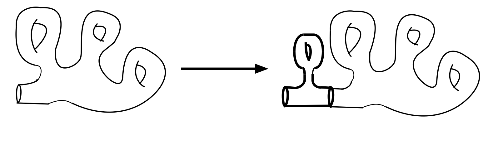
W ∪ θ ( W 1 , 2 ) ( + W e 1 ) Refer to caption
Figure 1. The above figure depicts the stabilization map. The submanifold W⊂[0,∞)×ℝ∞W\subset[0,\infty)\times\mathbb{R}^{\infty} is diffeomorphic to W3,1W_{3,1}. The stabilization map sends WW to the submanifold θ⁡(W1,2)∪(W+e1)⊂[0,∞)×ℝ∞\theta(W_{1,2})\cup(W+e_{1})\;\subset\;[0,\infty)\times\mathbb{R}^{\infty} which is diffeomorphic to W4,1W_{4,1}.

2.2. The Complex of Embedded Handles

We now construct a semi-simplicial space similar to the one constructed in [4, Definition 4.1]. We will need to construct a certain manifold as follows. Fix an oriented embedding

β:{1}×D2​n⟶∂W1,1.\beta:\{1\}\times D^{2n}\longrightarrow\partial W_{1,1}.

We define HH to be the manifold obtained from W1,1W_{1,1} by attaching [0,1]×D2​n[0,1]\times D^{2n} to W1,1W_{1,1} along the embedding β\beta, i.e. H:=W1,1∪βD2​n×[0,1]H:=W_{1,1}\cup_{\beta}D^{2n}\times[0,1].

We construct a core C⊂HC\subset H as follows. Recall that W1,1W_{1,1} is defined to be the manifold with boundary obtained from Sn×Sn+1S^{n}\times S^{n+1} by deleting the interior of an embedded open disk. Choose base points a0∈Sna_{0}\in S^{n} and b0∈Sn+1b_{0}\in S^{n+1} such that,

  1. (a)

    the subspace (Sn×{a0})∪({b0}×Sn+1)⊂Sn×Sn+1(S^{n}\times\{a_{0}\})\cup(\{b_{0}\}\times S^{n+1})\subset S^{n}\times S^{n+1} is contained in W1,1⊂Sn×Sn+1W_{1,1}\subset S^{n}\times S^{n+1},

  2. (b)

    the pair (a0,−b0)∈Sn×Sn+1(a_{0},-b_{0})\in S^{n}\times S^{n+1} is contained in W1,1W_{1,1}.

We then choose an embedded path γ\gamma in H=W1,1∪βD2​n×[0,1]H=W_{1,1}\cup_{\beta}D^{2n}\times[0,1] from the point (a0,−b0)(a_{0},-b_{0}) to (0,0)∈[0,1]×D2​n(0,0)\in[0,1]\times D^{2n} whose interior does not intersect

(Sn×{a0})∪({b0}×Sn+1)(S^{n}\times\{a_{0}\})\cup(\{b_{0}\}\times S^{n+1})

and whose image agrees with [0,1]×{0}⊂[0,1]×D2​n[0,1]\times\{0\}\subset[0,1]\times D^{2n}, inside [0,1]×D2​n[0,1]\times D^{2n}, see Fig. 2.

We then define CC to be the subspace of HH given by

C:=(Sn×{a0})∪({b0}×Sn+1)∪γ⁡([0,1])∪({0}×D2​n)⊂H.C:=(S^{n}\times\{a_{0}\})\cup(\{b_{0}\}\times S^{n+1})\cup\gamma([0,1])\cup(\{0\}\times D^{2n})\;\subset\;H.

It is immediate that CC is homotopy equivalent to to Sn∨Sn+1S^{n}\vee S^{n+1} and that furthermore CC is a deformation retract of HH.

× { 0 } D ⁢ 2 n × { a 0 } S + n 1 × S n { b 0 } γ ( [ 0 , 1 ] ) Refer to caption
Figure 2. Pictured above is the manifold H=[0,1]×D2​n∪βW1,1H=[0,1]\times D^{2n}\cup_{\beta}W_{1,1}. There is an embedding of the core, C=(Sn×{b0})∪({a0}×Sn+1)∪γ⁡([0,1])∪({0}×D2​n)C=(S^{n}\times\{b_{0}\})\cup(\{a_{0}\}\times S^{n+1})\cup\gamma([0,1])\cup(\{0\}\times D^{2n}), which is a deformation retraction of HH.

We choose an isotopy of embeddings

ρt:H⟶H\rho_{t}:H\longrightarrow H

defined for t∈[0,∞)t\in[0,\infty) which satisfies the following conditions:

  1. i.

    ρ0=I​dH\rho_{0}=Id_{H},

  2. ii.

    for any open neighborhood UU containing CC, there exists tU∈[0,∞)t_{U}\in[0,\infty) such that
    ρt​(H)⊂U\rho_{t}(H)\subset U for all t>tUt>t_{U},

  3. iii.

    for each t∈[0,∞)t\in[0,\infty) there is an open neighborhood VtV_{t} of CC such that ρt|Vt=I​dVt\rho_{t}|_{V_{t}}\;=\;Id_{V_{t}}.

Let WW be a compact (2​n+1)(2n+1)-dimensional manifold with ∂W≠∅\partial W\neq\emptyset, equipped with an embedding of a base coordinate patch

a:[0,1)×ℝ2​n⟶Wa:[0,1)\times\mathbb{R}^{2n}\longrightarrow W

such that a−1​(∂W)={0}×ℝ2​na^{-1}(\partial W)=\{0\}\times\mathbb{R}^{2n}. We define two semi-simplicial spaces K∙​(W,a)K_{\bullet}(W,a) and K∙δ​(W,a)K_{\bullet}^{\delta}(W,a) as follows.

Definition 2.2.

Let WW and a:[0,1)×ℝ2​n⟶Wa:[0,1)\times\mathbb{R}^{2n}\longrightarrow W be as above. The spaces of pp-simplices, Kp​(W,a)K_{p}(W,a) and Kpδ​(W,a)K^{\delta}_{p}(W,a) are defined as follows:

  1. (i)

    Let K0​(W,a)K_{0}(W,a) be the space of pairs (t,ϕ)(t,\phi), where t∈ℝt\in\mathbb{R} and ϕ:H⟶W\phi:H\longrightarrow W is an embedding for which there exists ϵ>0\epsilon>0 such that for (s,z)∈[0,ϵ)×D2​n⊂H(s,z)\in[0,\epsilon)\times D^{2n}\;\subset\;H,   ϕ⁡(s,z)=a⁡(s,z+t​e1)\phi(s,z)=a(s,z+te_{1}) where, e1∈ℝ2​ne_{1}\in\mathbb{R}^{2n} denotes the first basis vector.

  2. (ii)

    Let Kp​(W,a)⊂(K0​(W,a))p+1K_{p}(W,a)\subset(K_{0}(W,a))^{p+1} consist of those tuples ((t0,ϕ0),…,(tp,ϕp))((t_{0},\phi_{0}),\dots,(t_{p},\phi_{p})) such that t0<⋯<tpt_{0}<\cdots<t_{p} and the intersections ϕi​(C)∩ϕj​(C)\phi_{i}(C)\cap\phi_{j}(C) are empty for all i,j∈{0,…,p}i,j\in\{0,\dots,p\}.

The spaces Kp​(W,a)⊂(ℝ×Emb(H,W))pK_{p}(W,a)\subset(\mathbb{R}\times\Emb(H,W))^{p} are topologized using the C∞C^{\infty}-topology on the space of embeddings. Then the space Kpδ​(W,a)K^{\delta}_{p}(W,a) is defined so as to have the same underlying set as Kp​(W,a)K_{p}(W,a), but topologized using the discrete topology.

The assignments [p]↦Kp​(W,a)[p]\mapsto K_{p}(W,a) and [p]↦Kpδ​(W,a)[p]\mapsto K_{p}^{\delta}(W,a) define semi-simplicial spaces denoted by K∙​(W,a)K_{\bullet}(W,a) and K∙δ​(W,a)K_{\bullet}^{\delta}(W,a) respectively. Here the face maps di:Kp​(W,a)⟶Kp−1​(W,a)d_{i}:K_{p}(W,a)\longrightarrow K_{p-1}(W,a) for   0≤i≤p0\leq i\leq p are defined by sending a pp-tuple ((t0,ϕ0),…,(tp,ϕp))((t_{0},\phi_{0}),\dots,(t_{p},\phi_{p})) to the (p−1)(p-1)-tuple obtained by deleting the iith entry. The face maps di:Kpδ​(W,a)⟶Kp−1δ​(W,a)d_{i}:K^{\delta}_{p}(W,a)\longrightarrow K^{\delta}_{p-1}(W,a) are defined similarly.

We now define a simplicial complex Kc​(W,a)K^{c}(W,a) related to the semi-siplicial space K∙δ​(W,a)K^{\delta}_{\bullet}(W,a).

Definition 2.3.

Let Kc​(W,a)K^{c}(W,a) be the simplicial complex with the set of vertices identified with K0δ​(W,a)K^{\delta}_{0}(W,a). A set of vertices {(t0,ϕ0),…,(tp,ϕp)}\{(t_{0},\phi_{0}),\dots,(t_{p},\phi_{p})\}, is defined to be a pp-simplex in Kc​(W,a)K^{c}(W,a) if when written with t0≤⋯≤tpt_{0}\leq\cdots\leq t_{p}, the list ((t0,ϕ0),…,(tp,ϕp))((t_{0},\phi_{0}),\dots,(t_{p},\phi_{p})) is an element of Kpδ​(W,a)K^{\delta}_{p}(W,a).

Since a pp-simplex of K∙δ​(W,a)K^{\delta}_{\bullet}(W,a) is determined by its unordered set of vertices, there is a natural homeomorphism of geometric realizations:

(5) |K∙δ​(W,a)|≅|Kc​(W,a)|.|K^{\delta}_{\bullet}(W,a)|\cong|K^{c}(W,a)|.
Remark 2.1.

The semi-simplicial spaces K∙​(W,a)K_{\bullet}(W,a) and K∙δ​(W,a)K_{\bullet}^{\delta}(W,a) depend on the choice of embedding a:[0,1)×ℝ2​n⟶Wa:[0,1)\times\mathbb{R}^{2n}\longrightarrow W. However, it is easy to see that the homeomorphism type of their geometric realizations does not depend on the choice of aa. For the duration of the paper we will suppress aa from the notation and denote

K∙(W):=K∙(W,a),K∙δ(W):=K∙δ(W,a),andKc(W):=Kc(W,a).K_{\bullet}(W):=K_{\bullet}(W,a),\ \ \ K_{\bullet}^{\delta}(W):=K_{\bullet}^{\delta}(W,a),\ \ \ \mbox{and}\ \ \ K^{c}(W):=K^{c}(W,a).

3. The Algebraic Invariants

3.1. Intersection Products and Vector Bundles

In this section we develop in detail the algebraic invariants associated to an (n−1)(n-1)-connected, (2​n+1)(2n+1)-dimensional manifold that were introduced in the introduction. We first state Haefliger’s theorem from [6] which will allow us to identify the homotopy groups πn+1​(Wg,1)\pi_{n+1}(W_{g,1}) with the set of isotopy classes of embeddings of Sn+1S^{n+1} into Wg,1W_{g,1}.

Theorem 3.1.

(Haefliger, [6]) Let VV and MM be smooth manifolds with dim(V)=l\dim(V)=l and dim(M)=m\dim(M)=m. Suppose further that VV is (k−1)(k-1)-connected and that MM is kk-connected for some integer k≥0k\geq 0. Then,

  1. (a)

    Any continuous map of VV to MM is homotopic to a smooth embedding provided that m≥2​l−k+1m\geq 2l-k+1.

  2. (b)

    Any two smooth embeddings of VV into MM which are homotopic as continuous maps are smoothly isotopic provided that m≥2​l−k+2m\geq 2l-k+2.

Setting V=Sn+1V=S^{n+1} and M=Wg,1M=W_{g,1} yields the following corollary:

Corollary 3.2.

Let n≥4n\geq 4. Then πn+1​(Wg,1)\pi_{n+1}(W_{g,1}) and πn​(Wg,1)\pi_{n}(W_{g,1}) are each in bijective correspondence with set of isotopy classes of embeddings of Sn+1S^{n+1} and SnS^{n} into Wg,1W_{g,1} respectively.

Now, let MM be a kk-connected smooth manifold of dimension mm. Let rr and tt be positive integers less than or equal to the number min⁡{12​(m+k−2),m−2}.\min\{\frac{1}{2}(m+k-2),\;m-2\}. We study maps,

(6) λr,t:πr​(M)×πt​(M)⟶πr​(Sm−t)andαr:πr​(M)⟶πr−1​(S​Om−r)\lambda_{r,t}:\pi_{r}(M)\times\pi_{t}(M)\;\longrightarrow\;\pi_{r}(S^{m-t})\quad\text{and}\quad\alpha_{r}:\pi_{r}(M)\;\longrightarrow\;\pi_{r-1}(SO_{m-r})

which were defined by C.T.C. Wall in [10] as follows. For an embedding g:Sr⟶Mg:S^{r}\longrightarrow M (representing an element of πr​(M)\pi_{r}(M)), the class αr​([g])∈πr−1​(S​Om−r)\alpha_{r}([g])\in\pi_{r-1}(SO_{m-r}) is defined to be the element which classifies the normal bundle of gg. This is well defined because of Theorem 3.1; all homotopies of gg can be assumed to be isotopies of smooth embeddings.

Defining λr,t\lambda_{r,t} will take more work. Let

g:Sr⟶Mandf:St⟶Mg:S^{r}\longrightarrow M\quad\text{and}\quad f:S^{t}\longrightarrow M

be embeddings. Let Nf⊂MN_{f}\subset M denote a closed tubular neighborhood of f⁡(St)f(S^{t}) and let π:Nf⟶f⁡(St)\pi:N_{f}\longrightarrow f(S^{t}) denote the bundle projection. Let U⊂StU\subset S^{t} denote a closed neighborhood diffeomorphic to a disk. We set

V0:=π−1​(f⁡(U))andV1:=π−1​[f⁡(St)−int(f⁡(U))].V_{0}:=\pi^{-1}(f(U))\quad\text{and}\quad V_{1}:=\pi^{-1}[f(S^{t})-\Int(f(U))].

We define

Tf:[M−int(V0)]⟶Sm−tT_{f}:[M-\Int(V_{0})]\;\longrightarrow\;S^{m-t}

to be the Pontryagin-Thom map associated to the normal bundle π|V1:V1⟶(St−int(U)CLOSE\pi|_{V_{1}}:V_{1}\longrightarrow(S^{t}-\Int(U)). More precisely, letting φ:V1⟶≅Dt×Dm−t\varphi:V_{1}\stackrel{{\scriptstyle\cong}}{{\longrightarrow}}D^{t}\times D^{m-t} be a trivialization, and identifying Sm−tS^{m-t} with the push-out Dm−t∪c{∞}D^{m-t}\cup_{c}\{\infty\} (with c:Sm−t−1→{∞}c:S^{m-t-1}\rightarrow\{\infty\} the constant map), TfT_{f} is defined by the formula

(7) x↦{projDm−t​(ϕ​(x))if x∈V1∞if x∈[M−int(V0)]−V1.x\mapsto\begin{cases}\text{proj}_{D^{m-t}}(\phi(x))&\text{if $x\in V_{1}$}\\ \infty&\text{if $x\in\;[M-\Int(V_{0})]-V_{1}$.}\end{cases}

Clearly if ff and f′f^{\prime} are isotopic embeddings, then TfT_{f} and Tf′T_{f^{{}^{\prime}}} will be homotopic (the class of TfT_{f} does not depend on the choice of trivialization φ\varphi since the base-space is contractible). Since r≤m−2r\leq m-2 and V0≅DmV_{0}\cong D^{m}, the inclusion map i:M−int(V0)↪Mi:M-\Int(V_{0})\hookrightarrow M induces an isomorphism

i∗:πr​(M−int(V0))⟶≅πr​(M).i_{*}:\pi_{r}(M-\Int(V_{0}))\stackrel{{\scriptstyle\cong}}{{\longrightarrow}}\pi_{r}(M).

Finally, we define

(8) λr,t​([g],[f])=(Tf)∗∘i∗−1​[g].\lambda_{r,t}([g],[f])\;=\;(T_{f})_{*}\circ i_{*}^{-1}[g].

There is one more important map defined by C.T.C Wall in [10] which we need to use in order to compute the value of αr\alpha_{r} on certain isotopy classes. Let 2​m≥3​r+32m\geq 3r+3, m≥2​r−t+3m\geq 2r-t+3, and r≥tr\geq t. Then there is a map,

(9) F:πt−1​(S​Om−t)×πr​(St)⟶πr−1​(S​Om−r)F:\pi_{t-1}(SO_{m-t})\times\pi_{r}(S^{t})\longrightarrow\pi_{r-1}(SO_{m-r})

defined as follows. For (x,y)∈πt−1​(S​Om−t)×πr​(St)(x,y)\in\pi_{t-1}(SO_{m-t})\times\pi_{r}(S^{t}), let E⟶StE\longrightarrow S^{t} be the disk-bundle with fibre-dimension m−tm-t, classified by the element xx. Denote by i0:St→Ei_{0}:S^{t}\rightarrow E the zero section. If f:Sr⟶Stf:S^{r}\longrightarrow S^{t} is a map representing yy, the dimensional assumptions on t,r,t,r, and mm imply that the composition

Sr⟶fSt⟶i0ES^{r}\stackrel{{\scriptstyle f}}{{\longrightarrow}}S^{t}\stackrel{{\scriptstyle i_{0}}}{{\longrightarrow}}E

may be deformed to an embedding, which we denote by f^:Sr⟶E\widehat{f}:S^{r}\longrightarrow E. We then define F⁡(x,y)∈πr−1​(S​Om−r)F(x,y)\in\pi_{r-1}(SO_{m-r}) to be the element which classifies the normal bundle of f^​(Sr)\widehat{f}(S^{r}) in EE.

We will need an important result from [10] regarding this map FF.

Lemma 3.3.

(Wall, [10]) Let y∈πr​(St)y\in\pi_{r}(S^{t}) be in the image of the suspension map S:πr−1​(St−1)⟶πr​(St)S:\pi_{r-1}(S^{t-1})\longrightarrow\pi_{r}(S^{t}). Then the map πt−1​(S​Om−t)⟶πr−1​(S​Om−r)\pi_{t-1}(SO_{m-t})\longrightarrow\pi_{r-1}(SO_{m-r}) given by x↦F⁡(x,y)x\;\mapsto\;F(x,y) is a homomorphism.

The map FF can be used to compute the value of αr\alpha_{r} on homotopy classes of πr​(M)\pi_{r}(M) which can be factored as a composition Sr⟶fSt⟶gM.S^{r}\stackrel{{\scriptstyle f}}{{\longrightarrow}}S^{t}\stackrel{{\scriptstyle g}}{{\longrightarrow}}M. In this case, it follows directly from the definition of FF that

(10) αr​([g∘f])=F⁡(αt​([g]),[f]).\alpha_{r}([g\circ f])\;=\;F(\alpha_{t}([g]),\;[f]).

This formula will prove useful in the next section when computing the value of αn+1\alpha_{n+1} on πn+1​(Wg,1)\pi_{n+1}(W_{g,1}).

We now specialize to our main case of interest where MM is an (n−1)(n-1)-connected, (2​n+1)(2n+1)-manifold with n≥4n\geq 4. The map λn,n+1\lambda_{n,n+1} was defined using the Pontryagin-Thom construction and thus can be interpreted as an intersection invariant. It is easy to deduce:

Proposition 3.4.

For elements x∈πn​(M)x\in\pi_{n}(M) and y∈πn+1​(M)y\in\pi_{n+1}(M), let kx,y∈ℤk_{x,y}\in\mathbb{Z} be the signed intersection number for transversal embeddings which represent elements xx and yy. We have, λn,n+1​(x,y)=kx,y⋅ιn\lambda_{n,n+1}(x,\;y)\;=\;k_{x,y}\cdot\iota_{n} where ιn\iota_{n} is the standard generator of the group πn​(Sn)\pi_{n}(S^{n}).

Let xx and yy be as in the previous proposition and let f:Sn→Mf:S^{n}\rightarrow M and g:Sn+1→Mg:S^{n+1}\rightarrow M be transversal embeddings which represent xx and yy. Then by the Whitney Trick, [9, Theorem 6.6], one can find an isotopy hs:Sn+1⟶Mh_{s}:S^{n+1}\longrightarrow M, defined for s∈[0,1]s\in[0,1] with h0=gh_{0}=g and such that the image of h1h_{1} intersects the image of ff transversally at exactly |kx,y||k_{x,y}|-many points.

Now, let f:Sn+1→Mf:S^{n+1}\rightarrow M and g:Sn+1→Mg:S^{n+1}\rightarrow M be embeddings which intersect transversally. We will need a generalized version of the Whitney Trick that will enable us to construct an isotopy ht:Sn+1→Mh_{t}:S^{n+1}\rightarrow M such that h0=gh_{0}=g and h1​(Sn+1)∩f⁡(Sn+1)=∅h_{1}(S^{n+1})\cap f(S^{n+1})=\emptyset if and only if λn+1,n+1​([f],[g])=0\lambda_{n+1,n+1}([f],[g])=0. In [12] and [7], such generalized versions of the Whitney Trick were developed. We have:

Proposition 3.5.

(Wells, [12]) Let MM be an (n−1)(n-1)-connected, (2​n+1)(2n+1)-dimensional manifold. Let f:Sn+1⟶Mf:S^{n+1}\longrightarrow M and g:Sn+1⟶Mg:S^{n+1}\longrightarrow M be embeddings such that λn+1,n+1​([f],[g])=0\lambda_{n+1,n+1}([f],[g])=0. Then there is exists an isotopy ht:Sn+1→Mh_{t}:S^{n+1}\rightarrow M such that h0=gh_{0}=g and h1​(Sn+1)∩f⁡(Sn+1)=∅.h_{1}(S^{n+1})\cap f(S^{n+1})=\emptyset. Furthermore, if ff and gg are transversal and U⊂Sn+1U\subset S^{n+1} is an open disk containing g−1​(f⁡(Sn+1)∩g⁡(Sn+1))g^{-1}(f(S^{n+1})\cap g(S^{n+1})), then the isotopy hth_{t} may be chosen so that ht​(x)=g​(x)h_{t}(x)=g(x) for all x∈Sn+1∖Ux\in S^{n+1}\setminus U and t∈[0,1]t\in[0,1].

Remark 3.1.

This is a specialization of the main theorem of [12]. In [12] the author associates to sub-manifolds Ar,Bt⊂XmA^{r},B^{t}\subset X^{m} with ∂A,∂B⊂∂X\partial A,\partial B\subset\partial X and (∂A)∩(∂B)=∅(\partial A)\cap(\partial B)=\emptyset, an invariant valued in the stable homotopy group α⁡(A,B,X)∈πr+t−mS\alpha(A,B;X)\in\pi^{S}_{r+t-m} and proves that if certain dimensional and connectivity conditions are met, then there exists an isotopy ht:Ar→Xh_{t}:A^{r}\rightarrow X with h0=iAh_{0}=i_{A} and h1​(A)∩B=∅h_{1}(A)\cap B=\emptyset if and only if α⁡(A,B,X)=0\alpha(A,B;X)=0. Furthermore, it is proven that this isotopy can be chosen so as to be constant on ∂A\partial A. It can be easily checked that by setting A:=g⁡(Sn+1)A:=g(S^{n+1}), B:=f⁡(Sn+1)B:=f(S^{n+1}), and X:=MX:=M, the invariant α⁡(A,B,X)\alpha(A,B;X) is equal to λn+1,n+1​([f],[g])\lambda_{n+1,n+1}([f],[g]) after identifying πn+1​(Sn)\pi_{n+1}(S^{n}) (for OPENn≥4)n\geq 4) with π1S\pi_{1}^{S}.

We emphasize that with n≥4n\geq 4, the dimensional and connectivity conditions from the main theorem of [12] are satisfied. In order to construct such an isotopy hth_{t} that is constant outside of a neighborhood U⊂Sn+1U\subset S^{n+1} of g−1​(f⁡(Sn+1)∩g⁡(Sn+1))g^{-1}(f(S^{n+1})\cap g(S^{n+1})), we set A=g⁡(Sn+1−U)A=g(S^{n+1}-U), B=f⁡(Sn+1)B=f(S^{n+1}), and X=M−N⁡(U)X=M-N(U) where N⁡(U)⊂MN(U)\subset M is a tubular neighborhood of UU in MM. In this case α⁡(A,B,X)\alpha(A,B;X) is still equal to λn+1,n+1​([f],[g])\lambda_{n+1,n+1}([f],[g]), since λn+1,n+1​([f],[g])\lambda_{n+1,n+1}([f],[g]) was defined precisely by deleting such neighborhoods from Sn+1S^{n+1} and MM and then applying the Pontryagin-Thom construction (7).

We now state an important theorem regarding λn+1,n+1\lambda_{n+1,n+1} and αn+1\alpha_{n+1} which was proven in [10]. For what follows, denote by π:S​On+1⟶S​On+1/S​On≅Sn\pi:SO_{n+1}\longrightarrow SO_{n+1}/SO_{n}\cong S^{n} the projection map, denote by ∂:πn+1​(Sn)⟶πn​(S​On)\partial:\pi_{n+1}(S^{n})\longrightarrow\pi_{n}(SO_{n}) the boundary map in the long-exact sequence associated to the fibre-sequence S​On→S​On+1→SnSO_{n}\rightarrow SO_{n+1}\rightarrow S^{n}, and finally denote by S:πn​(Sn−1)→πn+1​(Sn)S:\pi_{n}(S^{n-1})\rightarrow\pi_{n+1}(S^{n}) the suspension map.

Theorem 3.6.

(Wall, [10]) Let MM be an (n−1)(n-1)-connected, (2​n+1)(2n+1)-dimensional manifold with n≥4n\geq 4. Then for x,y∈πn+1​(M)x,y\in\pi_{n+1}(M), we have

λn+1,n+1​(x,x)=S​π​αn+1​(x),\lambda_{n+1,n+1}(x,x)=S\pi\alpha_{n+1}(x),
αn+1​(x+y)=αn+1​(x)+αn+1​(y)+∂(λn+1,n+1​(x,y)).\alpha_{n+1}(x+y)\;=\;\alpha_{n+1}(x)+\alpha_{n+1}(y)+\partial(\lambda_{n+1,n+1}(x,y)).

Furthermore, λn+1,n+1\lambda_{n+1,n+1} is (−1)(n+1)(-1)^{(n+1)}-symmetric bilinear.

Here is one more useful result regarding λn,n+1\lambda_{n,n+1} and λn+1,n+1\lambda_{n+1,n+1} from [10].

Proposition 3.7.

(Wall, [10]) Let MM be an (n−1)(n-1)-connected, (2​n+1)(2n+1)-dimensional manifold with n≥4n\geq 4. Let f:Sn→Mf:S^{n}\rightarrow M and g:Sn+1→Mg:S^{n+1}\rightarrow M be embeddings and let β:Sn+1⟶Sn\beta:S^{n+1}\longrightarrow S^{n} be a map. Then λn+1,n+1​([f∘β],[g])=λn,n+1​([f],[g])∘[β].\lambda_{n+1,n+1}([f\circ\beta],\;[g])\;=\;\lambda_{n,n+1}([f],\;[g])\circ[\beta].

We will use these maps to deduce important information about the structure of HH and Wg,1W_{g,1}.

3.2. Calculations

We now compute the values of λn,n+1\lambda_{n,n+1}, λn+1,n+1\lambda_{n+1,n+1}, αn\alpha_{n}, and αn+1\alpha_{n+1} on the manifolds Wg,1W_{g,1}. Recall from the previous section the space,

H:=W1,1∪β[0,1]×D2​nH:=W_{1,1}\cup_{\beta}[0,1]\times D^{2n}

and the core C⊂HC\subset H used in Definition 2.2.

Denote by ιn\iota_{n} and ιn+1\iota_{n+1} the standard generators of πn​(Sn)\pi_{n}(S^{n}) and πn+1​(Sn+1)\pi_{n+1}(S^{n+1}) respectively. Recall that

πn+1​(Sn)≅{ℤif n=2ℤ/2if n≥3.\pi_{n+1}(S^{n})\cong\begin{cases}\mathbb{Z}&\text{if $n=2$}\\ \mathbb{Z}/2&\text{if $n\geq 3$.}\end{cases}

We then set ρn+1∈πn+1​(Sn)\rho_{n+1}\in\pi_{n+1}(S^{n}) to be the generator represented by the (n−2)(n-2)-fold suspension of the Hopf-Fibration S3→S2S^{3}\rightarrow S^{2}. Letting,

(11) jn:Sn↪C,jn+1:Sn+1↪C,andiC:C↪Hj_{n}:S^{n}\hookrightarrow C,\quad j_{n+1}:S^{n+1}\hookrightarrow C,\quad\text{and}\quad i_{C}:C\hookrightarrow H

denote the inclusions, we set

(12) e:=(iC∘jn)∗(ιn)∈πn(H),η:=(iC∘jn+1)∗(ιn+1)∈πn+1(H),\displaystyle e:=(i_{C}\circ j_{n})_{*}(\iota_{n})\;\in\pi_{n}(H),\quad\eta:=(i_{C}\circ j_{n+1})_{*}(\iota_{n+1})\;\in\pi_{n+1}(H),

and then

(13) μ:=e∘ρn+1∈πn+1​(H)\mu\;:=e\;\circ\rho_{n+1}\in\pi_{n+1}(H)

where, with some abuse of notation, e∘ρn+1e\circ\rho_{n+1} is the homotopy class of the composition of maps representing ee and ρn+1\rho_{n+1}. It is easy to see that

πn​(H)=⟨e⟩≅ℤandπn+1​(H)=⟨η,μ⟩≅ℤ⊕ℤ/2.\pi_{n}(H)=\langle e\rangle\cong\mathbb{Z}\quad\text{and}\quad\pi_{n+1}(H)=\langle\eta,\;\mu\rangle\cong\mathbb{Z}\oplus\mathbb{Z}/2.

We are now in a position to compute the values of λn,n+1\lambda_{n,n+1}, λn+1,n+1\lambda_{n+1,n+1}, αn\alpha_{n}, and αn+1\alpha_{n+1} on the homotopy groups of HH.

Proposition 3.8.

On the homotopy groups of HH, λn,n+1\lambda_{n,n+1}, λn+1,n+1\lambda_{n+1,n+1}, αn\alpha_{n}, and αn+1\alpha_{n+1} take the following values:

(14) αn​(e)=0\textstyle{\alpha_{n}(e)=0}αn+1​(η)=0\textstyle{\alpha_{n+1}(\eta)=0}αn+1​(μ)=0\textstyle{\alpha_{n+1}(\mu)=0}λn,n​(e,e)=0\textstyle{\lambda_{n,n}(e,e)=0}λn+1,n+1​(η,η)=0\textstyle{\lambda_{n+1,n+1}(\eta,\eta)=0}λn+1,n+1​(μ,μ)=0\textstyle{\lambda_{n+1,n+1}(\mu,\mu)=0}λn,n+1​(e,η)=ιn\textstyle{\lambda_{n,n+1}(e,\eta)=\iota_{n}}λn+1,n+1​(η,μ)=ρn+1\textstyle{\lambda_{n+1,n+1}(\eta,\mu)=\rho_{n+1}}λn,n+1​(e,μ)=0.\textstyle{\lambda_{n,n+1}(e,\mu)=0.}
Proof.

The calculations αn​(e)=0\alpha_{n}(e)=0 and αn+1​(η)=0\alpha_{n+1}(\eta)=0 follow from the fact that the embeddings iC∘jei_{C}\circ j_{e} and iC∘jηi_{C}\circ j_{\eta} from (11) which represent the classes ee and η\eta have trivial normal bundles. The calculation λn,n+1​(e,η)=ιn\lambda_{n,n+1}(e,\eta)=\iota_{n} follow from the fact that the embeddings iC∘jei_{C}\circ j_{e} and iC∘jηi_{C}\circ j_{\eta} intersect transversally at exactly one point.

To see that αn+1​(μ)=0\alpha_{n+1}(\mu)=0 we recall that μ\mu is defined by a composition, namely μ=e∘ρn+1\mu=e\circ\rho_{n+1}. From (10) we see that αn+1​(e∘ρn+1)=F⁡(αn​(e),ρn+1)=F⁡(0,ρn+1)\alpha_{n+1}(e\circ\rho_{n+1})=F(\;\alpha_{n}(e)\;,\;\rho_{n+1})=F(0,\;\rho_{n+1}). Since nn is assumed to be greater than or equal to 44, the element ρn+1\rho_{n+1} is a suspension, namely the (n−2)(n-2)-fold suspension of the Hopf fibration. From this, Lemma 3.3 implies that F⁡(⋅,ρn+1)F(\;\cdot\;,\;\rho_{n+1}) is linear in the first variable, hence F⁡(0,ρn+1)=0F(0,\rho_{n+1})=0, and so αn+1​(e∘ρn+1)= 0\alpha_{n+1}(e\circ\rho_{n+1})\;=\;0.

The calculation λn,n​(e,e)=0\lambda_{n,n}(e,e)=0 follows trivially from the fact that πn​(Sn+1)=0\pi_{n}(S^{n+1})=0. The calculation λn+1,n+1​(η,η)=0\lambda_{n+1,n+1}(\eta,\eta)=0 follows from the fact that αn+1​(η)=0\alpha_{n+1}(\eta)=0, using Theorem 3.6. The calculation λn+1,n+1​(μ,μ)=0\lambda_{n+1,n+1}(\mu,\mu)=0 follows from αn+1​(μ)=0\alpha_{n+1}(\mu)=0 using Theorem 3.6 as well.

Finally, to compute λn+1,n+1​(η,μ)\lambda_{n+1,n+1}(\eta,\mu) we use Proposition 3.7 to write,

λn+1,n+1​(η,μ)=λn+1,n+1​(η,e∘ρn+1)=λn+1,n​(η,e)∘ρn+1=ιn∘ρn+1=ρn+1.\lambda_{n+1,n+1}(\eta,\mu)\;=\;\lambda_{n+1,n+1}(\eta,e\circ\rho_{n+1})\;=\;\lambda_{n+1,n}(\eta,e)\circ\rho_{n+1}\;=\;\iota_{n}\circ\rho_{n+1}\;=\;\rho_{n+1}.

∎

We now compute the values of these invariants on πk​(Wg,1)\pi_{k}(W_{g,1}). Since Wg,1W_{g,1} is diffeomorphic to the boundary connect sum of gg-copies of W1,1W_{1,1} (or equivalently HH), we see that

πn​(Wg)≅(ℤ)⊕gandπn+1​(Wg,1)≅ℤ⊕g⊕(ℤ/2)⊕g.\pi_{n}(W_{g})\cong(\mathbb{Z})^{\oplus g}\quad\text{and}\quad\pi_{n+1}(W_{g,1})\;\cong\;\mathbb{Z}^{\oplus g}\oplus(\mathbb{Z}/2)^{\oplus g}.

Fix a (g−1)(g-1) simplex,

(15) {(ψ0,t0),…,(ψg−1,tg−1)}∈Kc​(Wg,1).\{(\psi_{0},t_{0}),\dots,(\psi_{g-1},t_{g-1})\}\in K^{c}(W_{g,1}).

Such a (g−1)(g-1)-simplex exists since the manifold Wg,1W_{g,1} is by construction diffeomorphic to the boundary connected sum of gg-many copies of HH. For i=0,…,g−1i=0,\dots,g-1, we set

ei:=(ψi)∗​(e)∈πn​(Wg,1),ηi:=(ψi)∗​(η)∈πn+1​(Wg,1),μi:=(ψi)∗​(μ)∈πn+1​(Wg,1).e_{i}:=(\psi_{i})_{*}(e)\in\pi_{n}(W_{g,1}),\quad\eta_{i}:=(\psi_{i})_{*}(\eta)\in\pi_{n+1}(W_{g,1}),\quad\mu_{i}:=(\psi_{i})_{*}(\mu)\in\pi_{n+1}(W_{g,1}).
Proposition 3.9.

On the homotopy groups of Wg,1W_{g,1}, the maps λr,t\lambda_{r,t} and αr\alpha_{r} take the following values:

(16) αn​(ei)=0\textstyle{\alpha_{n}(e_{i})=0}αn+1​(ηi)=0\textstyle{\alpha_{n+1}(\eta_{i})=0}αn+1​(μi)=0\textstyle{\alpha_{n+1}(\mu_{i})=0}λn,n+1​(ei,ηj)=δi,j⋅ιn\textstyle{\lambda_{n,n+1}(e_{i},\eta_{j})=\delta_{i,j}\cdot\iota_{n}}λn,n​(ei,ej)=0\textstyle{\lambda_{n,n}(e_{i},e_{j})=0}λn+1,n+1​(ηi,ηj)=0\textstyle{\lambda_{n+1,n+1}(\eta_{i},\eta_{j})=0}λn+1,n+1​(ηj,μi)=δi,j⋅ρn+1\textstyle{\lambda_{n+1,n+1}(\eta_{j},\mu_{i})=\delta_{i,j}\cdot\rho_{n+1}}λn+1,n+1​(μi,μj)=0\textstyle{\lambda_{n+1,n+1}(\mu_{i},\mu_{j})=0}λn,n+1​(ei,μj)=0.\textstyle{\lambda_{n,n+1}(e_{i},\mu_{j})=0.}
Proof.

This follows directly from the previous proposition combined with the fact that the intersection ψi​(C)∩ψj​(C)=∅\psi_{i}(C)\cap\psi_{j}(C)=\emptyset for all i,j∈{0,…​g−1}i,j\in\{0,\dots g-1\}. ∎

3.3. Wall Pairings

We now formalize the algebraic structure given by the 55-tuple,

(πn​(H),πn+1​(H),λn,n+1,λn+1,n+1,αn+1).(\pi_{n}(H),\;\pi_{n+1}(H),\;\lambda_{n,n+1},\;\lambda_{n+1,n+1},\;\alpha_{n+1}).

For an integer g≥0g\geq 0, let XX and YY be ℤ\mathbb{Z}-modules (not necessarily free) of rank gg. Let

λ:X×Y⟶πn​(Sn),q:Y×Y⟶πn+1​(Sn),α:Y⟶πn​(S​On)\lambda:X\times Y\longrightarrow\pi_{n}(S^{n}),\quad q:Y\times Y\longrightarrow\pi_{n+1}(S^{n}),\quad\alpha:Y\longrightarrow\pi_{n}(SO_{n})

be maps such that λ\lambda is bilinear, qq is symmetric bilinear, and α\alpha is a function (not necessarily a homomorphism) that satisfies the relation

(17) α⁡(a+b)=α⁡(a)+α⁡(b)+∂(q⁡(a,b))​for all a,b∈Y.\alpha(a+b)=\alpha(a)+\alpha(b)+\partial(q(a,b))\;\;\text{for all $a,b\in Y$}.

The main example of such maps arise by setting X:=πn​(M)X:=\pi_{n}(M) and Y:=πn+1​(M)Y:=\pi_{n+1}(M) for MM an (n−1)(n-1)-connected, (2​n+1)(2n+1)-dimensional manifold, and setting the maps λ,q,\lambda,q, and α\alpha equal to λn,n+1,λn+1,n+1,\lambda_{n,n+1},\lambda_{n+1,n+1}, and αn+1\alpha_{n+1} as defined in Section 3.1 (we are ignoring αn\alpha_{n} here since in our case of interest it is identically zero). We now impose further conditions on X,Y,λ,q,X,\;Y,\;\lambda,\;q, and α\alpha.

Definition 3.1.

Let X,Y,λ,q,X,\;Y,\;\lambda,\;q, and α\alpha be as defined above with

X≅ℤ⊕gandY≅ℤ⊕g⊕(ℤ/2)⊕g.X\cong\mathbb{Z}^{\oplus g}\quad\text{and}\quad Y\cong\mathbb{Z}^{\oplus g}\oplus(\mathbb{Z}/2)^{\oplus g}.

Suppose further that there exist bases

(x1,…,xg)and(y1,…,yg,z1,…,zg)(x_{1},\dots,x_{g})\quad\text{and}\quad(y_{1},\dots,y_{g},z_{1},\dots,z_{g})

of XX and YY respectively with (z1,…,zg)(z_{1},\dots,z_{g}) a basis for the ℤ/2\mathbb{Z}/2-component of YY, such that for all i,j∈{1,…,g}i,j\in\{1,\dots,g\} the following conditions are satisfied:

  1. i.

    λ⁡(xi,yj)=δi,j⋅ιn\lambda(x_{i},y_{j})=\delta_{i,j}\cdot\iota_{n} and λ⁡(xi,zj)=0\lambda(x_{i},z_{j})=0,

  2. ii.

    q⁡(yi,zj)=q⁡(zj,yi)=δi,j⋅ρn+1q(y_{i},z_{j})=q(z_{j},y_{i})=\delta_{i,j}\cdot\rho_{n+1} and q⁡(yi,yj)=q⁡(zi,zj)=0q(y_{i},y_{j})=q(z_{i},z_{j})=0,

  3. iii.

    α⁡(yi)=α⁡(zi)=0\alpha(y_{i})=\alpha(z_{i})=0.

These conditions determine the values of the functions λ,q\lambda,q, and α\alpha. With these conditions satisfied, the 55-tuple (X,Y,λ,q,α)(X,\;Y,\;\lambda,\;q,\;\alpha) is said to be a Wall pairing of rank gg.

It follows immediately from the calculation of Proposition 3.8 that

(18) (πn​(H),πn+1​(H),λn,n+1,λn+1,n+1,αn+1)(\pi_{n}(H),\;\pi_{n+1}(H),\;\lambda_{n,n+1},\;\lambda_{n+1,n+1},\;\alpha_{n+1})

is a Wall pairing of rank 11. It follows from Proposition 3.8 that the bases (e)(e) and (η,μ)(\eta,\mu), and maps λn,n+1,λn+1,n+1\lambda_{n,n+1},\lambda_{n+1,n+1}, and αn+1\alpha_{n+1}, satisfy of the conditions put forth the Definition 3.1. It then follows from Proposition 3.9 that

(πn​(Wg,1),πn+1​(Wg,1),λn,n+1,λn+1,n+1,αn+1)(\pi_{n}(W_{g,1}),\;\pi_{n+1}(W_{g,1}),\;\lambda_{n,n+1},\;\lambda_{n+1,n+1},\;\alpha_{n+1})

is a Wall pairing of rank gg.

Homorphisms and direct sums of Wall pairings are defined in the obvious way. We state without proof the easy to verify but important proposition:

Proposition 3.10.

Any Wall pairing of rank one is isomorphic to the Wall pairing (18). Furthermore, any Wall pairing of rank gg is isomorphic to the gg-fold direct sum of the Wall pairings (18).

By this proposition we are justified in thinking of a rank gg Wall pairing as an algebraic version of the manifold Wg,1W_{g,1}.

Let (X,Y,λ,q,α)(X,\;Y,\;\lambda,\;q,\;\alpha) be a Wall pairing of rank gg. It follows from Definition 3.1 that λ:X×Y⟶πn​(Sn)\lambda:X\times Y\longrightarrow\pi_{n}(S^{n}) is a perfect pairing , i.e. the map

X⟶Hom(Y,πn​(Sn)),x↦λ⁡(x,⋅)X\longrightarrow\Hom(Y,\pi_{n}(S^{n})),\quad x\mapsto\lambda(x,\;\cdot\;)

is an isomorphism. The bilinear pairing q:Y×Y⟶πn+1​(Sn)q:Y\times Y\longrightarrow\pi_{n+1}(S^{n}) enjoys a similar property.

Proposition 3.11.

Let Y′⊂YY^{\prime}\subset Y be any compliment to Torsion(Y)\Torsion(Y) in YY. Then the map

Torsion(Y)⟶Hom(Y′,πn+1​(Sn)),z↦q⁡(z,⋅)\Torsion(Y)\longrightarrow\Hom(Y^{\prime},\pi_{n+1}(S^{n})),\quad z\mapsto q(z,\;\cdot\;)

is an isomorphism.

Proof.

Let (y1,…,yg,z1,…,zg)(y_{1},\dots,y_{g},z_{1},\dots,z_{g}) be a basis of YY which satisfies conditions i., ii., and iii. in Definition 3.1 and denote by Y′′Y^{\prime\prime} the free sub ℤ\mathbb{Z}-module generated by (y1,…,yg)(y_{1},\dots,y_{g}). Since Torsion​(Y)\text{Torsion}(Y) is generated by (z1,…,zg)(z_{1},\dots,z_{g}), it is immediate from Definition 3.1 that the map

Torsion​(Y)⟶Hom(Y′′,πn+1​(Sn)),z↦q⁡(z,⋅)\text{Torsion}(Y)\longrightarrow\Hom(Y^{\prime\prime},\pi_{n+1}(S^{n})),\quad z\mapsto q(z,\;\cdot\;)

is an isomorphism. Let π:Y⟶Y′\pi:Y\longrightarrow Y^{\prime} be the projection map defined by the direct-sum decomposition, Y′⊕Torsion​(Y)=YY^{\prime}\oplus\text{Torsion}(Y)=Y. For dimensional reasons the restriction map, π|Y′′:Y′′⟶Y′\pi|_{Y^{\prime\prime}}:Y^{\prime\prime}\longrightarrow Y^{\prime} is an isomorphism. Since q⁡(z,z′)=0q(z,z^{\prime})=0 whenever both z,z′z,z^{\prime} are in Torsion​(Y)\text{Torsion}(Y) it follows that

q⁡(z,y)=q⁡(z,π⁡(y))for all z∈Torsion​(Y) and y∈Y′′.q(z,y)\;=\;q(z,\pi(y))\quad\text{for all $z\in\text{Torsion}(Y)$ and $y\in Y^{\prime\prime}$}.

This implies that the diagram

Torsion(Y)\textstyle{\Torsion(Y)\ignorespaces\ignorespaces\ignorespaces\ignorespaces\ignorespaces\ignorespaces\ignorespaces\ignorespaces}≅\scriptstyle{\cong}Hom(Y′′,πn+1​(Sn))\textstyle{\Hom(Y^{\prime\prime},\pi_{n+1}(S^{n}))\ignorespaces\ignorespaces\ignorespaces\ignorespaces}≅\scriptstyle{\cong}(π|Y′)∗\scriptstyle{(\pi|_{Y^{\prime}})^{*}}Hom(Y′,πn+1​(Sn))\textstyle{\Hom(Y^{\prime},\pi_{n+1}(S^{n}))}

commutes. This proves the proposition. ∎

It follows from the previous proposition that if (y1,…,yg)(y_{1},\dots,y_{g}) is a unimodular list of elements in YY spanning a free direct summand of rank gg such that α⁡(yi)=0\alpha(y_{i})=0 for all ii, then there exist unique bases, (x1,…,xg)(x_{1},\dots,x_{g}) and (z1,…,zg)(z_{1},\dots,z_{g}) for XX and Torsion​(Y)\text{Torsion}(Y) respectively such that the lists

(x1,…,xg)and(y1,…,yg,z1,…,zg)(x_{1},\dots,x_{g})\quad\text{and}\quad(y_{1},\dots,y_{g},z_{1},\dots,z_{g})

satisfy conditions i., ii., and iii. in Definition 3.1. This observation leads to the following proposition:

Proposition 3.12.

Let (X,Y,λ,q,α)(X,\;Y,\;\lambda,\;q,\;\alpha) be a Wall pairing of rank gg. There exists a unique map

ρ:X⟶Torsion​(Y)\rho:X\longrightarrow\mbox{{\rm Torsion}}(Y)

that satisfies,

(19) q⁡(ρ⁡(x),y)=λ⁡(x,y)∘ρn+1for all (x,y)∈X×Yq(\rho(x),\;y)\;=\;\lambda(x,y)\circ\rho_{n+1}\quad\text{for all $(x,y)\in X\times Y$}

where ρn+1∈πn+1​(Sn)\rho_{n+1}\in\pi_{n+1}(S^{n}) is the standard generator.

Proof.

Let (y1,…,yg)(y_{1},\dots,y_{g}) be a unimodular list of elements in YY spanning a free direct summand of rank gg such that α⁡(yi)=0\alpha(y_{i})=0 for all ii. Then let (x1,…,xg)(x_{1},\dots,x_{g}) and (z1,…,zg)(z_{1},\dots,z_{g}) be the unique bases of XX and Torsion​(Y)\text{Torsion}(Y) so that

(x1,…,xg)and(y1,…,yg,z1,…,zg)(x_{1},\dots,x_{g})\quad\text{and}\quad(y_{1},\dots,y_{g},z_{1},\dots,z_{g})

satisfy conditions i., ii., and iii. in Definition 3.1. We define ρ:X⟶Y\rho:X\longrightarrow Y to be the homomorphism determined by xi↦zix_{i}\mapsto z_{i} for i=1,…,gi=1,\dots,g. Clearly with this definition ρ\rho satisfies (19). Uniqueness of the map ρ\rho follows from uniqueness of the complimentary bases (x1,…,xg)(x_{1},\dots,x_{g}) and (z1,…,zg)(z_{1},\dots,z_{g}) to the unimodular sequence (y1,…,yg)(y_{1},\dots,y_{g}). ∎

For the Wall pairing (πn​(Wg,1),πn+1​(Wg,1),λn,n+1,λn+1,n+1,αn+1)(\pi_{n}(W_{g,1}),\;\pi_{n+1}(W_{g,1}),\;\lambda_{n,n+1},\;\lambda_{n+1,n+1},\;\alpha_{n+1}), the map ρ\rho is given by the formula, x↦x∘ρn+1x\mapsto x\circ\rho_{n+1} for x∈πn​(Wg,1)x\in\pi_{n}(W_{g,1}). This is indeed a homomorphism since when n≥4n\geq 4, the homotopy group πn+1​(Wg,1)\pi_{n+1}(W_{g,1}) is in the stable range.

This map ρ:X⟶Torsion​(Y)\rho:X\longrightarrow\text{Torsion}(Y) will prove to be useful latter on when working with Wall pairings.

4. High Connectivity of K∙​(Wg,1)K_{\bullet}(W_{g,1})

In this section we prove that the geometric realization |K∙​(Wg,1)||K_{\bullet}(W_{g,1})| is highly connected. We do so by comparing it to a highly connected simplicial complex Kπ​(Wg,1)K^{\pi}(W_{g,1}) modeled on the Wall pairing (πn​(Wg,1),πn+1​(Wg,1),λn,n+1,λn+1,n+1,αn+1)(\pi_{n}(W_{g,1}),\;\pi_{n+1}(W_{g,1}),\;\lambda_{n,n+1},\;\lambda_{n+1,n+1},\;\alpha_{n+1}) described in the previous section.

Definition 4.1.

Let (X,Y,λ,q,α)(X,\;Y,\;\lambda,\;q,\;\alpha) be a Wall pairing. We define K⁡(X,Y,λ,q,α)K(X,\;Y,\;\lambda,\;q,\;\alpha) to be the simplicial complex whose pp-simplices are given by sets of pairs

{(x0,y0),…,(xp,yp)}⊂X×Y\{(x_{0},y_{0}),\dots,(x_{p},y_{p})\}\subset X\times Y

such that for i,j=0,…,pi,j=0,\dots,p the following conditions are satisfied:

  1. i.

    λ⁡(xi,yj)=δi,j⋅ιn\lambda(x_{i},y_{j})=\delta_{i,j}\cdot\iota_{n},

  2. ii.

    q⁡(yi,yj)=0q(y_{i},y_{j})=0,

  3. iii.

    α⁡(yi)=0\alpha(y_{i})=0.

By the above definition, each vertex (x,y)∈K⁡(X,Y,λ,q,α)(x,y)\in K(X,\;Y,\;\lambda,\;q,\;\alpha) determines an embedding of the rank 11 Wall pairing determined by the restrictions of λ,q\lambda,q, and α\alpha to the submodules ⟨x⟩⊂X\langle x\rangle\subset X and ⟨y,ρ⁡(x)⟩⊂Y\langle y,\;\rho(x)\rangle\subset Y. The main Wall pairing that we are interested in is of course

(πn​(Wg,1),πn+1​(Wg,1),λn,n+1,λn+1,n+1,αn+1).(\pi_{n}(W_{g,1}),\;\pi_{n+1}(W_{g,1}),\;\lambda_{n,n+1},\;\lambda_{n+1,n+1},\;\alpha_{n+1}).

In order to save space we will denote,

(20) Kπ​(Wg,1):=K⁡(πn​(Wg,1),πn+1​(Wg,1),λn,n+1,λn+1,n+1,αn+1).K^{\pi}(W_{g,1})\;:=\;K(\pi_{n}(W_{g,1}),\;\pi_{n+1}(W_{g,1}),\;\lambda_{n,n+1},\;\lambda_{n+1,n+1},\;\alpha_{n+1}).

We view the complex Kπ​(Wg,1)K^{\pi}(W_{g,1}) as an algebraic version of the complex Kc​(Wg,1)K^{c}(W_{g,1}).

To prove our main theorem, we will need the complex Kπ​(Wg,1)K^{\pi}(W_{g,1}) to have a certain technical property. Recall the definition from [4]:

Definition 4.2.

A simplicial complex KK is said to be weakly Cohen-Macaulay of dimension nn if it is (n−1)(n-1)-connected and the link of any pp-simplex is (n−p−2)(n-p-2)-connected. In this case, we write ω​C​M​(K)≥n\omega CM(K)\geq n.

There is a general theorem from [4] regarding weakly Cohen-Macaulay complexes which we will need. We state the theorem here.

Theorem 4.1.

(Galatius and Randal-Williams, [4, Theorem 2.4]) Let XX be a simplicial complex and f:∂In⟶|X|f:\partial I^{n}\longrightarrow|X| be a map which is simplicial with respect to some PL triangulation of ∂In\partial I^{n}. Then, if ω​C​M​(X)≥n\omega CM(X)\geq n, the triangulation extends to a PL triangulation of InI^{n}, and ff extends to a simplicial map g:In⟶|X|g:I^{n}\longrightarrow|X| with the property that g⁡(link(v))⊂link(g⁡(v))g(\link(v))\subset\link(g(v)) for each interior vertex v∈In−∂Inv\in I^{n}-\partial I^{n}. In particular, gg is simplexwise injective if ff is.

We now state a theorem whose proof we put off until Section 5.

Theorem 4.2.

For g>3g>3, ω​C​M​(Kπ​(Wg,1))≥12​(g−1)\omega CM(K^{\pi}(W_{g,1}))\geq\frac{1}{2}(g-1).

It follows from this theorem that the geometric realization |Kπ​(Wg,1)||K^{\pi}(W_{g,1})| is 12​(g−3)\frac{1}{2}(g-3)-connected.

Recall from the previous section the elements e∈πn​(H)e\in\pi_{n}(H) and η∈πn+1​(H)\eta\in\pi_{n+1}(H). There is a simplicial map

(21) Kc​(Wg,1)⟶Kπ​(Wg,1),(ϕ,t)↦(ϕ∗​(e),ϕ∗​(η)).K^{c}(W_{g,1})\longrightarrow K^{\pi}(W_{g,1}),\quad(\phi,t)\;\mapsto\;(\phi_{*}(e),\;\phi_{*}(\eta)).

Recall that for any simplex ((ϕ0,t0),…,(ϕp,tp))((\phi_{0},t_{0}),\dots,(\phi_{p},t_{p})) the cores ϕ0​(C),…,ϕp​(C)\phi_{0}(C),\dots,\phi_{p}(C) are disjoint. Thus the above map respects adjacencies and is actually a simplicial map. We will prove that this map is highly connected.

Theorem 4.3.

Let n:=12​[dim(Wg,1)−1]n:=\frac{1}{2}[\dim(W_{g,1})-1] be greater than or equal to 44. Then the map Kc​(Wg,1)⟶Kπ​(Wg,1)K^{c}(W_{g,1})\longrightarrow K^{\pi}(W_{g,1}) from (21) is 12​(g−3)\frac{1}{2}(g-3)-connected.

Proof.

Let k≤12​(g−3)k\leq\frac{1}{2}(g-3) and consider a map f:Sk⟶|Kc​(Wg,1)|f:S^{k}\longrightarrow|K^{c}(W_{g,1})|, which we may assume is simplicial with respect to some PL triangulation of Sk=∂Ik+1S^{k}=\partial I^{k+1}. By Theorem 4.2 the composition ∂Ik+1⟶|Kc​(Wg,1)|⟶|Kπ​(Wg,1)|\partial I^{k+1}\longrightarrow|K^{c}(W_{g,1})|\longrightarrow|K^{\pi}(W_{g,1})| is null homotopic and so extends to a map g:Ik+1⟶|Kπ​(Wg,1)|g:I^{k+1}\longrightarrow|K^{\pi}(W_{g,1})|, which we may suppose is simplicial with respect to a PL triangulation of Ik+1I^{k+1} extending the triangulation of its boundary.

By Lemma 4.2, OPENω​C​M​(Kπ))≥12​(g−1)\omega CM(K^{\pi}))\geq\frac{1}{2}(g-1) and so by Theorem 4.1, as k+1≤12​(g−1)k+1\leq\frac{1}{2}(g-1), we can arrange that gg is simplexwise injective on the interior of Ik+1I^{k+1}. We choose a total order on the interior vertices of Ik+1I^{k+1} and inductively choose lifts of each vertex to Kc​(Wg,1)K^{c}(W_{g,1}) which respect adjacencies.

Let (x,y)(x,y) be a vertex in the image of the interior of Ik+1I^{k+1} under the map gg. We have x∈πn​(Wg,1)x\in\pi_{n}(W_{g,1}) and y∈πn+1​(Wg,1)y\in\pi_{n+1}(W_{g,1}) such that

α(x)=0,α(y)=0,andλn,n+1(x,y)=ιn∈πn(Sn).\alpha(x)=0,\quad\alpha(y)=0,\quad\text{and}\quad\lambda_{n,n+1}(x,y)=\iota_{n}\in\pi_{n}(S^{n}).

Furthermore, the elements xx and yy can be represented by embeddings of spheres, Sn+1S^{n+1} and SnS^{n}, each with trivialized normal bundle. Since λn,n+1​(x,y)=ιn\lambda_{n,n+1}(x,y)=\iota_{n}, application of the Whitney Trick implies that we may assume that these embedded spheres representing xx and yy intersect each other transversally at exactly one point. Using a general position argument, we may then assume that xx and yy are represented by embeddings,

jx:Sn+1×Dn⟶Wg,1andjy:Dn+1×Sn⟶Wg,1j_{x}:S^{n+1}\times D^{n}\longrightarrow W_{g,1}\quad\text{and}\quad j_{y}:D^{n+1}\times S^{n}\longrightarrow W_{g,1}

such that

jx​(Sn+1×Dn)∩jy​(Dn+1×Sn)=U×Vj_{x}(S^{n+1}\times D^{n})\cap j_{y}(D^{n+1}\times S^{n})\;=\;U\times V

where U⊂jx​(Sn+1×{0})U\subset j_{x}(S^{n+1}\times\{0\}) and V⊂jy​({0}×Sn)V\subset j_{y}(\{0\}\times S^{n}) are submanifolds (embedded as closed subsets), diffeomorphic to Dn+1D^{n+1} and DnD^{n} respectively. It can be easily checked that the push-out

(22) Mx,y:=jx​(Sn+1×Dn)​⋃U×Vjy​(Dn+1×Sn)M_{x,y}:=j_{x}(S^{n+1}\times D^{n})\bigcup_{U\times V}j_{y}(D^{n+1}\times S^{n})

is diffeomorphic to W1,1=Sn+1×Sn−int(D2​n+1)W_{1,1}=S^{n+1}\times S^{n}-\Int(D^{2n+1}), after smoothing the corners. The inclusion of Mx,yM_{x,y} from (22) determines an embedding W1,1↪Wg,1W_{1,1}\hookrightarrow W_{g,1}. One then chooses an embedded arc connecting Mx,yM_{x,y} to ∂Wg,1\partial W_{g,1} whose interior has empty intersection with Mx,yM_{x,y} and ∂Wg,1\partial W_{g,1} (this is possible by a general position argument). A thickening of this ark together with the embedding W1,1↪Wg,1W_{1,1}\hookrightarrow W_{g,1} then determines an embedding ϕ:H⟶Wg,1\phi:H\longrightarrow W_{g,1} and thus a lift of the vertex (x,y)(x,y) to a vertex in Kc​(Wg,1)K^{c}(W_{g,1}). This takes care of the zeroth step of the induction.

Now suppose that (x,y)(x,y) is an interior vertex and let (x1,y1),…,(xk,yk)(x_{1},y_{1}),\dots,(x_{k},y_{k}) be the vertices adjacent to (x,y)(x,y) that have already been lifted and denote by (ϕ1,t1),…,(ϕk,tk)(\phi_{1},t_{1}),\dots,(\phi_{k},t_{k}) their lifts. Note that the set {(x1,y1),…,(xk,yk)}\{(x_{1},y_{1}),\dots,(x_{k},y_{k})\} is not necessarily a simplex in Kπ​(Wg,1)K^{\pi}(W_{g,1}). However, {(x,y),(xj,yj)}\{(x,y),(x_{j},y_{j})\} is a 11-simplex in Kπ​(Wg,1)K^{\pi}(W_{g,1}) for j=1,…,kj=1,\dots,k. Now,

λn,n+1(x,yj)=0,λn,n+1(xj,y)=0,andλn+1,n+1(y,yj)=0for j=1,…,k\lambda_{n,n+1}(x,y_{j})=0,\quad\lambda_{n,n+1}(x_{j},y)=0,\quad\text{and}\quad\lambda_{n+1,n+1}(y,y_{j})=0\quad\text{for $j=1,\dots,k$}

and so we may apply the Whitney Trick and its generalization Proposition 3.5 inductively, to choose embeddings

jx:Sn⟶Wg,1andjy:Sn+1⟶Wg,1j_{x}:S^{n}\longrightarrow W_{g,1}\quad\text{and}\quad j_{y}:S^{n+1}\longrightarrow W_{g,1}

representing the classes xx and yy such that jx​(Sn)j_{x}(S^{n}) and jy​(Sn+1)j_{y}(S^{n+1}) are disjoint form the cores ϕj​(C)\phi_{j}(C) (recall Section 2.2), for all j∈{1,…,k}j\in\{1,\dots,k\}. Furthermore, since λn,n+1​(x,y)=ιn\lambda_{n,n+1}(x,y)=\iota_{n}, we may by application of the Whitney Trick assume further that jxj_{x} and jyj_{y} are such that jx​(Sn)j_{x}(S^{n}) and jy​(Sn+1)j_{y}(S^{n+1}) intersect transversally at just one point. We then carry out the plumbing construction employed in the zeroth step of the induction on the embeddings jxj_{x} and jyj_{y} to obtain an embedding ϕ:H⟶Wg,1\phi:H\longrightarrow W_{g,1} such that ϕ⁡(C)∩ϕj​(C)=∅\phi(C)\cap\phi_{j}(C)=\emptyset for all j∈{1,…,k}j\in\{1,\dots,k\}. This completes the induction and proves the theorem. ∎

It follows from the above theorem that |Kc​(Wg,1)||K^{c}(W_{g,1})| is 12​(g−3)\frac{1}{2}(g-3)-connected. Now, since every simplex of the semi-simplicial set K∙δ​(Wg,1)K^{\delta}_{\bullet}(W_{g,1}) is determined entirely by its vertices, there is a homeomorphism |Kc​(Wg,1)|≅|K∙δ​(Wg,1)||K^{c}(W_{g,1})|\cong|K^{\delta}_{\bullet}(W_{g,1})|, and thus |K∙δ​(Wg,1)||K^{\delta}_{\bullet}(W_{g,1})| is 12​(g−3)\frac{1}{2}(g-3)-connected as well.

We now consider the natural map K∙δ​(Wg,1)⟶K∙​(Wg,1)K^{\delta}_{\bullet}(W_{g,1})\longrightarrow K_{\bullet}(W_{g,1}).

Lemma 4.4.

The semi-simplical space K∙​(Wg,1)K_{\bullet}(W_{g,1}) is 12​(g−3)\frac{1}{2}(g-3)-connected.

Proof.

This is proven in exactly the same way as [4, Theorem 4.6]. The theorem is based entirely on simplicial techniques and has no dependence on the structure of the manifolds present. ∎

We now derive two important corollaries of the previous lemma. These are both proven in the same way as [4, Corollary 4.4] and [4, Corollary 4.5].

Corollary 4.5.

(Transitivity). Suppose that g≥3g\geq 3 and let ϕ0,ϕ1:H↪Wg,1\phi_{0},\phi_{1}:H\hookrightarrow W_{g,1} be embeddings. Then there is a diffeomorphism ff of Wg,1W_{g,1} which is isotopic to the identity on the boundary and such that ϕ1=f∘ϕ0\phi_{1}=f\circ\phi_{0}.

Proof.

Suppose first that ϕ0\phi_{0} and ϕ1\phi_{1} are disjoint. Let VV denote the closure of a regular neighborhood of ϕ0​(H)∪ϕ1​(H)∪∂Wg,1\phi_{0}(H)\cup\phi_{1}(H)\cup\partial W_{g,1}. The submanifold VV is abstractly diffeomorphic to W2,2W_{2,2} (which is by definition (#2Sn+1×Sn)−[int(D2​n+1⊔int(D2​n+1)](\#^{2}S^{n+1}\times S^{n})-[\Int(D^{2n+1}\sqcup\Int(D^{2n+1})]) and has two standard copies of HH embedded in it, both connected to the first component of the boundary. With this assumption that ϕ0\phi_{0} and ϕ1\phi_{1} are disjoint, it is enough to find a diffeomorphism of W2,2W_{2,2} which is the identity on the first boundary component, is isotopic to the identity on the second boundary component, and sends the first embedded copy of HH to the second.

We give an explicit construction of such a diffeomorphism. For what follows we use the standard model of S2​n⊂ℝ2​n+1S^{2n}\subset\mathbb{R}^{2n+1} given by

S2​n={(x1,…,x2​n+1)∈ℝ2​n+1|x12+⋯+x2​n+12=1}.S^{2n}=\{(x_{1},\dots,x_{2n+1})\in\mathbb{R}^{2n+1}\;|\;x_{1}^{2}+\cdots+x_{2n+1}^{2}=1\}.

We equip [0,1]×S2​n[0,1]\times S^{2n} with the metric obtained by taking the product of the Euclidean metric on [0,1][0,1], and the metric on S2​nS^{2n} induced from the Euclidean metric on ℝ2​n+1\mathbb{R}^{2n+1}. Now, let Γ∈S​O​(2​n+1)\Gamma\in SO(2n+1) be the diagonal matrix with entries (−1,−1,1,…,1)(-1,-1,1,\dots,1). Let d0:D2​n+1→[0,1]×S2​nd_{0}:D^{2n+1}\rightarrow[0,1]\times S^{2n} be the embedding of a disk of radius 14\frac{1}{4} centered at the point (12,(1,0,…,0))∈[0,1]×S2​n(\tfrac{1}{2},(1,0,\dots,0))\in[0,1]\times S^{2n}. We then set d1:=(I​d[0,1]×Γ)∘d0d_{1}:=(Id_{[0,1]}\times\Gamma)\circ d_{0}. It is immediate that d1d_{1} is an embedding of a disk of radius 14\frac{1}{4} centered at the point (12,(−1,0,…,0))∈[0,1]×S2​n(\tfrac{1}{2},(-1,0,\dots,0))\in[0,1]\times S^{2n}. We form a manifold denoted by M2,2M_{2,2}, by connect summing two copies of Sn×Sn+1S^{n}\times S^{n+1} to [0,1]×S2​n[0,1]\times S^{2n} at the disks d0​(D2​n+1)d_{0}(D^{2n+1}) and d1​(D2​n+1)d_{1}(D^{2n+1}),

M2,2=(Sn×Sn+1)​#d0​([0,1]×S2​n)​#d1​(Sn×Sn+1).M_{2,2}=(S^{n}\times S^{n+1})\#_{d_{0}}([0,1]\times S^{2n})\#_{d_{1}}(S^{n}\times S^{n+1}).

Clearly M2,2M_{2,2} is abstractly diffeomorphic to W2,2W_{2,2}. There is a diffeomorphism φ\varphi of M2,2M_{2,2} which is equal to I​d[0,1]×ΓId_{[0,1]}\times\Gamma on [0,1]×S2​n∖(d0​(D2​n+1)∪d1​(D2​n+1))[0,1]\times S^{2n}\setminus(d_{0}(D^{2n+1})\cup d_{1}(D^{2n+1})), and interchanges the two copies of Sn×Sn+1−int​(D2​n+1)S^{n}\times S^{n+1}-\text{int}(D^{2n+1}). There is an embedded copy of HH given by union the first copy of Sn×Sn+1−int​(D2​n+1)S^{n}\times S^{n+1}-\text{int}(D^{2n+1}) with a thickening of the arc [12,1]×{(1,0,…,0)}[\frac{1}{2},1]\times\{(1,0,\dots,0)\}, and its image under φ\varphi gives another disjoint embedded copy of HH. The diffeomorphism φ\varphi, by construction interchanges the two embedded copies of HH, however φ\varphi is not the identity map on the boundary component {0}×S2​n\{0\}\times S^{2n}. To fix this, we replace I​d[0,1]×ΓId_{[0,1]}\times\Gamma in the above construction with a function of the form

(t,x)↦(t,γ⁡(t)⋅x)for (t,x)∈[0,1]×S2​n(t,x)\;\mapsto\;(t,\gamma(t)\cdot x)\quad\text{for $(t,x)\in[0,1]\times S^{2n}$}

where γ:[0,1]→S​O​(2​n+1)\gamma:[0,1]\rightarrow SO(2n+1) is a path in S​O​(2​n+1)SO(2n+1) which is the identity on [0,ϵ][0,\epsilon] and Γ\Gamma on [2​ϵ,1][2\epsilon,1] for 0<ϵ<180<\epsilon<\frac{1}{8}.

Now suppose that ϕ0\phi_{0} and ϕ1\phi_{1} are not disjoint. We put an equivalence relation on the vertices of Kc​(Wg,1)K^{c}(W_{g,1}). We define two vertices, (ϕ0,t0)(\phi_{0},t_{0}) and (ϕ1,t1)(\phi_{1},t_{1}) to be equivalent if there exists a diffeomorphism ff of Wg,1W_{g,1}, isotopic to the identity on the boundary, such that f∘ϕ0=ϕ1f\circ\phi_{0}=\phi_{1}. The previous paragraph implies that two such vertices are equivalent if ϕ0\phi_{0} and ϕ1\phi_{1} are disjoint, or equivalently if the set {(ϕ0,t0),(ϕ1,t1)}\{(\phi_{0},t_{0}),(\phi_{1},t_{1})\} is a 11-simplex in the complex Kc​(Wg,1)K^{c}(W_{g,1}). If g≥3g\geq 3, Theorem 4.3 implies that |Kc​(Wg,1)||K^{c}(W_{g,1})| is path-connected, hence any two vertices are connected via a zig-zag of 11-simplices. It follows that any two vertices of Kc​(Wg,1)K^{c}(W_{g,1}) are equivalent by our equivalence relation. ∎

Corollary 4.6.

(Cancelation) Let MM be a (2​n+1)(2n+1)-dimensional manifold with boundary parametrized by S2​nS^{2n}, and suppose there is a diffeomorphism

φ:M​#​(Sn×Sn+1)⟶Wg+1,1\varphi:M\#(S^{n}\times S^{n+1})\longrightarrow W_{g+1,1}

which is the identity on the boundary. Then if g≥3g\geq 3 there is a diffeomorphism of MM with Wg,1W_{g,1} which is the identity on the boundary, with respect to the parametrization by S2​nS^{2n}.

Proof.

Recall from Section 2.2 that (H=[0,1]×D2​n)∪βW1,1(H=[0,1]\times D^{2n})\cup_{\beta}W_{1,1} where β:{1}×D2​n→∂W1,1\beta:\{1\}\times D^{2n}\rightarrow\partial W_{1,1} is an embedding. Choose an embedding

γ:H⟶Wg+1,1\gamma:H\longrightarrow W_{g+1,1}

which satisfies γ⁡({0}×D2​n)⊂∂Wg+1,1\gamma(\{0\}\times D^{2n})\subset\partial W_{g+1,1}, and such that there exists a diffeomorphism

Cl​(Wg+1,1−γ⁡(H))≅Wg,1\text{Cl}(W_{g+1,1}-\gamma(H))\cong W_{g,1}

where Cl denotes the closure. Notice that since Wg,1W_{g,1} is diffeomorphic to the boundary-connect-sum of g+1g+1 copies of HH, one can simply choose γ\gamma to be the embedding given by inclusion of the last factor of HH in the boundary-connect-sum decomposition.

From the connect sum M​#​(Sn×Sn+1)M\#(S^{n}\times S^{n+1}), there is a cannonical embedding

j:W1,1↪M​#​(Sn×Sn+1).j:W_{1,1}\hookrightarrow M\#(S^{n}\times S^{n+1}).

By choosing a thickening of an arc which connects j⁡(∂W1,1)j(\partial W_{1,1}) to the boundary of the manifold M​#​(Sn×Sn+1)M\#(S^{n}\times S^{n+1}), we obtain an extension of j:W1,1↪M​#​(Sn×Sn+1)j:W_{1,1}\hookrightarrow M\#(S^{n}\times S^{n+1}) to an embedding

f:H⟶M​#​(Sn+1×Sn)f:H\longrightarrow M\#(S^{n+1}\times S^{n})

with f⁡({0}×D2​n)⊂∂(M​#​(Sn+1×Sn))f(\{0\}\times D^{2n})\subset\partial(M\#(S^{n+1}\times S^{n})). It follows from the construction of ff, together with the fact that the boundary of M​#​(Sn+1×Sn)M\#(S^{n+1}\times S^{n}) is diffeomorphic to S2​nS^{2n}, that there is a diffeomorphism

Cl​(M​#​(Sn×Sn+1)−f⁡(H))≅M−int(D2​n+1).\text{Cl}(M\#(S^{n}\times S^{n+1})-f(H))\;\cong\;M-\Int(D^{2n+1}).

With φ:M​#​(Sn×Sn+1)⟶Wg+1,1\varphi:M\#(S^{n}\times S^{n+1})\longrightarrow W_{g+1,1} the diffeomorphism from the statement of the corollary, we have two embeddings

φ∘f:H⟶Wg+1,1andγ:H⟶Wg+1,1.\varphi\circ f:H\longrightarrow W_{g+1,1}\quad\text{and}\quad\gamma:H\longrightarrow W_{g+1,1}.

By Corollary 4.5 there is a diffeomorphism qq of Wg+1,1W_{g+1,1} isotopic to the identity on the boundary so that γ=q∘φ∘f\gamma=q\circ\varphi\circ f. We then obtain a diffeomorphism

q∘φ:M​#​(Sn×Sn+1)⟶Wg+1,1q\circ\varphi:M\#(S^{n}\times S^{n+1})\;\longrightarrow\;W_{g+1,1}

such that the composition

γ−1∘q∘φ∘f:H⟶H\gamma^{-1}\circ q\circ\varphi\circ f:H\longrightarrow H

is the identity map. In particular, it maps the submanifold W1,1⊂HW_{1,1}\subset H to itself identically. So then, after removing the interiors of f⁡(W1,1)f(W_{1,1}) and γ⁡(W1,1)\gamma(W_{1,1}), the restriction of q∘φq\circ\varphi yields a diffeomorphism,

M−int(D2​n+1)\textstyle{M-\Int(D^{2n+1})\ignorespaces\ignorespaces\ignorespaces\ignorespaces}≅\scriptstyle{\cong}Wg,1−int(D2​n+1)\textstyle{W_{g,1}-\Int(D^{2n+1})}

which is equal to the identity on the new boundary component corresponding to the removed disk, and is isotopic to the identity on the old boundary component (with respect to the parametrization by S2​nS^{2n}). We may then fill in the new boundary component with a disk and use isotopy extension to make the diffeomorphism be the identity, with respect to the parametrization by S2​nS^{2n}, on the remaining boundary component. ∎

In the final section we will need the following modification of K∙​(Wg,1)K_{\bullet}(W_{g,1}).

Definition 4.3.

Let K¯∙​(Wg,1)⊂K∙​(Wg,1)\bar{K}_{\bullet}(W_{g,1})\subset K_{\bullet}(W_{g,1}) be the sub-semi-simplicial space consisting of all simplices ((ϕ0,t0),…,(ϕp,tp))((\phi_{0},t_{0}),\dots,(\phi_{p},t_{p})) such that the intersections ϕi​(H)∩ϕj​(H)\phi_{i}(H)\cap\phi_{j}(H) are empty for all i,j∈{0,…,p}i,j\in\{0,\dots,p\}.

Corollary 4.7.

The space |K¯∙​(Wg,1)||\bar{K}_{\bullet}(W_{g,1})| is 12​(g−3)\frac{1}{2}(g-3)-connected.

Proof.

Precomposing with the isotopy ρt\rho_{t}, any tuple of embeddings with disjoint cores eventually becomes disjoint. It follows that the inclusion K¯∙​(Wg,1)↪K∙​(Wg,1)\bar{K}_{\bullet}(W_{g,1})\hookrightarrow K_{\bullet}(W_{g,1}) is a level-wise weak equivalence. ∎

5. High-Connectivity of the Complex Kπ​(Wg,1)K^{\pi}(W_{g,1})

In this section we prove Theorem 4.2. This theorem is about the simplicial complex Kπ​(Wg,1)K^{\pi}(W_{g,1}). However, it will be convenient for our purposes to work with partially ordered sets instead of simplicial complexes.

We review the relationship between simplicial complexes, semi-simplicial sets, and posets. Let KK be a simplicial complex. Associated to KK is the semi-simplical set K∙K_{\bullet} whose pp-simplices are the injective simplicial maps △p→K\triangle^{p}\rightarrow K, i.e. ordered (p+1)(p+1)-tuples of vertices in KK spanning a pp-simplex. There is a natural surjection |K∙|→|K||K_{\bullet}|\rightarrow|K|, and any choice of total order on the set of vertices of KK induces a section |K|→|K∙||K|\rightarrow|K_{\bullet}|. In particular, |K||K| is at least as connected as |K∙||K_{\bullet}|. Associated to the semi-simplicial set K∙K_{\bullet} is a poset denoted by K^∙\widehat{K}_{\bullet} whose elements are the simplices of K∙K_{\bullet} and the ordering is given by setting σ≤αif di1∘⋯∘dik(α)=σ\sigma\leq\alpha\quad\text{if \; $d_{i_{1}}\circ\cdots\circ d_{i_{k}}(\alpha)\;=\;\sigma$} for some sequence i1,…,iki_{1},\dots,i_{k}, i.e. σ≤α\sigma\leq\alpha if σ\sigma is a face of α\alpha. We must now define the geometric realization of a poset.

Definition 5.1.

Let EE any poset. We define |E||E| to be the geometric realization of the semi-simplicial set whose pp-simplices are the ordered (p+1)(p+1)-tuples x0<x1<⋯<xpx_{0}<x_{1}<\cdots<x_{p} of elements of EE. We will refer to |E||E| as the geometric realization of of the poset EE.

As above, let K^∙\widehat{K}_{\bullet} denote the poset associated to the semi-simplicial space K∙K_{\bullet}. It is easy to check that the geometric realization |K^∙||\widehat{K}_{\bullet}| is the barycentric sub-division of |K∙||K_{\bullet}|. In particular, there is a homotopy equivalence |K^∙|∼|K∙|.|\widehat{K}_{\bullet}|\sim|K_{\bullet}|.

From the above discussion it follows that in order to prove that |Kπ​(Wg,1)||K^{\pi}(W_{g,1})| is 12​(g−3)\frac{1}{2}(g-3)-connected, it will suffice to prove that the geometric realization of the associated poset K^∙π​(Wg,1)\widehat{K}^{\pi}_{\bullet}(W_{g,1}) is 12​(g−3)\frac{1}{2}(g-3)-connected.

Notational Convention 5.1.

If KK is a simplicial complex we will denote by K∙K_{\bullet} the semi-simplicial complex associated to KK and we will denote by K^∙\widehat{K}_{\bullet} the poset associated to K∙K_{\bullet}. For any poset EE we will denote by |E||E| the geometric realization as defined in Definition 5.1.

5.1. Some Basic Results About Posets

We now review from [2] some basic results on posets that we will need in order to prove that the poset K^∙π​(Wg,1)\widehat{K}^{\pi}_{\bullet}(W_{g,1}) is 12​(g−3)\frac{1}{2}(g-3)-connected. We use many of the constructions and results from [2] and use much of the same notation.

For a poset EE and an element x∈Ex\in E, we denote,

E<x:={y∈E|y<x},\displaystyle E_{<x}:=\{y\in E\;|\;y<x\}, E>x:={y∈E|y>x},\displaystyle E_{>x}:=\{y\in E\;|\;y>x\},
E≤x:={y∈E|y≤x},\displaystyle E_{\leq x}:=\{y\in E\;|\;y\leq x\}, E≥x:={y∈E|y≥x}.\displaystyle E_{\geq x}:=\{y\in E\;|\;y\geq x\}.

It is immediate that E<x,E<x,E<xE_{<x},E_{<x},E_{<x}, and E<xE_{<x} are all sub-posets of EE.

For any set XX, we denote by 𝒪⁡(X)\mathcal{O}(X) the poset comprised of non-empty, finite, ordered lists of distinct elements in XX. The partial ordering is given by setting,

(w1,…,wj)≤(v1,…,vk)(w_{1},\dots,w_{j})\leq(v_{1},\dots,v_{k})

if (w1,…,wj)(w_{1},\dots,w_{j}) is an ordered sub-list of (v1,…,vk)(v_{1},\dots,v_{k}). We say that a sub-poset F⊂𝒪⁡(X)F\subset\mathcal{O}(X) satisfies the chain condition if

  1. i.

    v∈Fv\in F implies 𝒪​(X)<v⊂F\mathcal{O}(X)_{<v}\subset F, and

  2. ii

    v∈Fv\in F implies every permutation of the sequence v=(v1,…,vk)v=(v_{1},\dots,v_{k}) is in FF.

If x<wx<w in 𝒪⁡(X)\mathcal{O}(X), let w∖xw\setminus x denote the subsequence of ww complimentary to xx. Let F⊆𝒪⁡(X)F\subseteq\mathcal{O}(X) be a sub-poset and let v:=(v1,…,vk)v:=(v_{1},\dots,v_{k}) be an element of 𝒪⁡(X)\mathcal{O}(X). We define

Fv\displaystyle F_{v} :={(w1,…,wj)∈F|(w1,…,wj,v1,…,vk)∈F}\displaystyle:=\;\{(w_{1},\dots,w_{j})\in F\;|\;(w_{1},\dots,w_{j},v_{1},\dots,v_{k})\in F\}
Zn​F\displaystyle Z^{n}F :={w∈𝒪⁡(X⊔{z1,…,zn})|(z1,…,zn)<w​and​w∖z∈F}.\displaystyle:=\;\{w\in\mathcal{O}(X\sqcup\{z_{1},\dots,z_{n}\})\;|\;(z_{1},\dots,z_{n})<w\;\text{and}\;w\setminus z\in F\}.

The posets FvF_{v} and Zn​FZ^{n}F arrise when studying the link of a vertex in |F||F|. In particular, the link of vv in |F||F| is the geometric realization of the poset

linkF​(v)={w∈F|v<w​or​v>w}=F<v⋆F>v\text{link}_{F}(v)\;=\;\{w\in F\;|\;v<w\;\text{or}\;v>w\}\;=\;F_{<v}\star F_{>v}

where ⋆\star denotes the join. If FF satisfies the chain condition, then |F<v||F_{<v}| is homeomorphic to a (k−2)(k-2)-sphere and F>vF_{>v} is isomorphic to Zk​(Fv)Z^{k}(F_{v}), with isomorphism given by sending viv_{i} to ziz_{i}. Hence there is a homeomorphism of geometric realizations

(23) |linkF​(v)|≅Σk−1​|Zk​Fv|.|\text{link}_{F}(v)|\;\cong\;\Sigma^{k-1}|Z^{k}F_{v}|.

For a non-empty set SS, define

F⁡⟨S⟩={((w1,s1),…,(wj,sj))∈𝒪⁡(X×S)|(w1,…,wj)∈F}.F\langle S\rangle\;=\;\{((w_{1},s_{1}),\dots,(w_{j},s_{j}))\in\mathcal{O}(X\times S)\;|\;(w_{1},\dots,w_{j})\in F\}.

If v=(v1,…,vk)∈𝒪⁡(X)v=(v_{1},\dots,v_{k})\in\mathcal{O}(X), let |v|=k=(length of v).|v|=k=(\text{length of $v$}). We now state several technical lemmas. See [2] and [3] for details. For the following we assume that F⊂𝒪⁡(X)F\subset\mathcal{O}(X) satisfies the chain condition.

Lemma 5.1.

For any v∈Fv\in F, the inclusion |Fv|↪|F||F_{v}|\hookrightarrow|F| is nullhomotopic.

Lemma 5.2.

Suppose dd is an integer such that for any v∈Fv\in F, FvF_{v} is (d−|v|)(d-|v|)-connected and FF is min​(1,d−1)\text{min}(1,d-1)-connected. Let s0∈Ss_{0}\in S. Then the maps,

in:F⟶Zn​F,\displaystyle i_{n}:F\longrightarrow Z^{n}F, (v1,…,vk)↦(v1,…,vk,z1,…,zn),\displaystyle(v_{1},\dots,v_{k})\mapsto(v_{1},\dots,v_{k},z_{1},\dots,z_{n}),
(s0)∗:F⟶F⁡⟨S⟩,\displaystyle(s_{0})_{*}:F\longrightarrow F\langle S\rangle, (v1,…,vk)↦((v1,s0),…,(vk,s0)),\displaystyle(v_{1},\dots,v_{k})\mapsto((v_{1},s_{0}),\dots,(v_{k},s_{0})),
in∘(s0)∗:F⟶Zn​(F⁡⟨S⟩)\displaystyle i_{n}\circ(s_{0})_{*}:F\longrightarrow Z^{n}(F\langle S\rangle)

induce isomorphisms on homotopy groups πj\pi_{j} for j≤dj\leq d.

Lemma 5.3.

Suppose Y⊆XY\subseteq X. If dd is an integer such that F∩𝒪⁡(Y)F\cap\mathcal{O}(Y) is dd-connected and Fv∩𝒪⁡(Y)F_{v}\cap\mathcal{O}(Y) is (d−|v|)(d-|v|)-connected for all v∈Fv\in F, then FF is dd-connected.

5.2. The Main Theorem

Now we proceed to prove Theorem 4.2. The first step here is to construct a poset model for the complex K∙π​(Wg,1)K^{\pi}_{\bullet}(W_{g,1}).

Definition 5.2.

Let (X,Y,λ,q,α)(X,\;Y,\;\lambda,\;q,\;\alpha) be a Wall pairing. We define

L⁡(X,Y,λ,q,α)⊂𝒪⁡(X×Y)L(X,\;Y,\;\lambda,\;q,\;\alpha)\subset\mathcal{O}(X\times Y)

to be the sub-poset of 𝒪⁡(X×Y)\mathcal{O}(X\times Y) consisting of sequences ((x1,y1),…,(xk,yk))((x_{1},y_{1}),\dots,(x_{k},y_{k})) such that for all i,j∈{1,…,k}i,j\in\{1,\dots,k\}:

  1. i.

    λ⁡(xi,yj)=δi,j⋅ιn\lambda(x_{i},y_{j})=\delta_{i,j}\cdot\iota_{n},

  2. ii.

    q⁡(yi,yj)=0q(y_{i},y_{j})=0,

  3. iii.

    α⁡(yi)=0\alpha(y_{i})=0.

When the context is clear we will suppress λ,q,\lambda,q, and α\alpha from the notation and denote

L⁡(X,Y):=L⁡(X,Y,λ,q,α).L(X,\;Y)\;:=\;L(X,\;Y,\;\lambda,\;q,\;\alpha).

By the discussion from the beginning of Section 5 and from the fact that all rank gg Wall pairings are isomorphic, it is clear that if (X,Y,λ,q,α)(X,\;Y,\;\lambda,\;q,\;\alpha) is a rank gg Wall pairing, then the geometric realization |L⁡(X,Y)||L(X,Y)| is homeomorphic to the barycentric subdivision of the space |K∙π​(Wg,1)||K^{\pi}_{\bullet}(W_{g,1})| (recall, K∙π​(Wg,1)K^{\pi}_{\bullet}(W_{g,1}) is the semi-simplicial space determined by the simplicial complex Kπ​(Wg,1)K^{\pi}(W_{g,1})).

The main step in proving Theorem 4.2 will be to prove the following:

Theorem 5.4.

Let (X,Y,λ,q,α)(X,\;Y,\;\lambda,\;q,\;\alpha) be a Wall pairing of rank gg. Then the geometric realization |L⁡(X,Y)||L(X,Y)| is 12​(g−3)\frac{1}{2}(g-3)-connected.

It follows from this theorem that the space |Kπ​(Wg,1)||K^{\pi}(W_{g,1})| is 12​(g−3)\frac{1}{2}(g-3)-connected. We will need some auxiliary constructions.

Definition 5.3.

For any free ℤ\mathbb{Z}-module VV, Let U⁡(V)⊂𝒪⁡(V)U(V)\subset\mathcal{O}(V) denote the poset consisting of sequences (x1,…,xk)(x_{1},\dots,x_{k}) of elements of VV which are unimodular, i.e. the sub ℤ\mathbb{Z}-module spanned by (x1,…,xk)(x_{1},\dots,x_{k}) splits as a direct summand of VV.

We will need to use the following important theorem from [8, Section 2].

Theorem 5.5.

(W. Van der Kallen, [8]) Let VV be a free ℤ\mathbb{Z}-module of rank gg. Then the geometric realization |U⁡(V)||U(V)| is (g−3)(g-3)-connected. Furthermore, if v∈U⁡(V)v\in U(V) then the geometric realization |U​(V)v||U(V)_{v}| is (g−3−|v|)(g-3-|v|)-connected.

This result will play a crucial role in our proof of Theorem 5.4. We now define new poset which will allow us to compare the poset L⁡(X,Y)L(X,Y) to the poset U⁡(X)U(X) for any Wall pairing (X,Y,λ,q,α)(X,Y,\lambda,q,\alpha).

Definition 5.4.

For a Wall-pairing (X,Y,λ,q,α)(X,Y,\lambda,q,\alpha), we define

M⁡(X,Y):=M⁡(X,Y,λ,q,α)M(X,Y):=M(X,Y,\lambda,q,\alpha)

to be the sub-poset of 𝒪⁡(X×Y)\mathcal{O}(X\times Y) consisting of sequences ((x1,y1),…,(xk,yk))((x_{1},y_{1}),\dots,(x_{k},y_{k})) subject to the following conditions:

  1. i.

    the list (x1,…,xk)(x_{1},\dots,x_{k}) is an element of U⁡(X)U(X),

  2. ii.

    α⁡(yi)=0\alpha(y_{i})=0 for all i∈{1,…,k}i\in\{1,\dots,k\},

  3. iii.

    for each ii, either yi=0y_{i}=0 or λ⁡(xj,yi)=δi,j⋅ιn\lambda(x_{j},y_{i})=\delta_{i,j}\cdot\iota_{n} for all j∈{1,…,k}j\in\{1,\dots,k\},

  4. iv.

    q⁡(yi,yj)=0q(y_{i},y_{j})=0 for all i,j∈{1,…,k}i,j\in\{1,\dots,k\}.

We will need to use one more important result about Wall pairings. For a Wall pairing (X,Y,λ,q,α)(X,\;Y,\;\lambda,\;q,\;\alpha) of rank gg, let V⊂XV\subset X and W⊂YW\subset Y be free sub-ℤ\mathbb{Z}-modules of rank k>0k>0 that each split as direct summands of XX and YY, such that the restriction

λ|V×W:V×W⟶πn​(Sn)\lambda|_{V\times W}:V\times W\longrightarrow\pi_{n}(S^{n})

is a perfect pairing. Denote,

(24) V⟂\displaystyle V^{\perp} ={y∈Y|λ⁡(v,y)=0​for all v∈V},\displaystyle=\;\{y\in Y\;|\;\lambda(v,y)=0\;\text{for all $v\in V$}\},
W⟂\displaystyle W^{\perp} ={x∈X|λ⁡(x,w)=0​for all w∈W},\displaystyle=\;\{x\in X\;|\;\lambda(x,w)=0\;\text{for all $w\in W$}\},
W^\displaystyle\widehat{W} ={y∈W|q⁡(y,w)=0​for all w∈W}.\displaystyle=\;\{y\in W\;|\;q(y,w)=0\;\text{for all $w\in W$}\}.

Denote by λ′\lambda^{\prime}, q′q^{\prime}, and α′\alpha^{\prime} the restrictions of the maps λ,q,\lambda,q, and α\alpha to W⟂W^{\perp} and V⟂∩W^V^{\perp}\cap\widehat{W}.

Lemma 5.6.

Let (X,Y,λ,q,α)(X,\;Y,\;\lambda,\;q,\;\alpha), V⊂XV\subset X, and W⊂YW\subset Y be as above. The tuple

(W⟂,V⟂∩W^,λ′,q′,α′)(W^{\perp},\;V^{\perp}\cap\widehat{W},\;\lambda^{\prime},\;q^{\prime},\;\alpha^{\prime})

is a Wall pairing of rank g−kg-k.

Proof.

In order to prove the lemma it will suffice to find a ℤ\mathbb{Z}-basis (x1,…,xg−k)(x_{1},\dots,x_{g-k}) of W⟂W^{\perp} and a unimodular sequence (y1,…,yg−k)(y_{1},\dots,y_{g-k}) of elements of V⟂∩W^V^{\perp}\cap\widehat{W} such that for all i,j∈{1,…,g−k}i,j\in\{1,\dots,g-k\} the following conditions are met:

  1. (a)

    λ⁡(xi,yj)=δi,j⋅ιn\lambda(x_{i},y_{j})\;=\;\delta_{i,j}\cdot\iota_{n},

  2. (b)

    q⁡(yi,yj)=0q(y_{i},y_{j})=0,

  3. (c)

    α⁡(yi)=0\alpha(y_{i})=0,

  4. (d)

    λ⁡(v,yi)=0\lambda(v,y_{i})=0 q⁡(yi,w)=0q(y_{i},w)=0 for all v∈Vv\in V, w∈Ww\in W.

We will then show that,

⟨y1,…,yg−k⟩⊕⟨ρ⁡(x1),…,ρ⁡(xg−k)⟩=(V⟂∩W^),\langle y_{1},\dots,y_{g-k}\rangle\oplus\langle\rho(x_{1}),\dots,\rho(x_{g-k})\rangle\;=\;(V^{\perp}\cap\widehat{W}),

where recall from Proposition 3.12 that ρ:X⟶Torsion​(Y)\rho:X\longrightarrow\text{Torsion}(Y) is the unique homomorphism such that q⁡(ρ⁡(x),y)=λ⁡(x,y)∘ρn+1q(\rho(x),y)\;=\;\lambda(x,y)\circ\rho_{n+1} for all (x,y)∈X×Y(x,y)\in X\times Y. This implies

(x1,…,xg−k)and(y1,…,yg−k,ρ⁡(x1),…,ρ⁡(xg−k))(x_{1},\dots,x_{g-k})\quad\text{and}\quad(y_{1},\dots,y_{g-k},\rho(x_{1}),\dots,\rho(x_{g-k}))

are bases of W⟂W^{\perp} and V⟂∩W^V^{\perp}\cap\widehat{W} which satisfy conditions i., ii., and iii. of Definition 3.1, thus implying that the tuple (W⟂,V⟂∩W^,λ′,q′,α′)(W^{\perp},\;V^{\perp}\cap\widehat{W},\;\lambda^{\prime},\;q^{\prime},\;\alpha^{\prime}) is indeed a Wall pairing.

Since (X,Y,λ,q,α)(X,Y,\lambda,q,\alpha) is a Wall pairing, it follows that there exists a free sub-ℤ\mathbb{Z}-module Y0⊂YY_{0}\subset Y with Y=Y0⊕Torsion​(Y)Y\;=\;Y_{0}\oplus\text{Torsion}(Y), such that

α⁡(Y0)=0andq⁡(Y0×Y0)=0.\alpha(Y_{0})=0\quad\text{and}\quad q(Y_{0}\times Y_{0})=0.

Since λ′:V×W⟶πn​(Sn)\lambda^{\prime}:V\times W\longrightarrow\pi_{n}(S^{n}), the restriction of λ\lambda as above, is by hypothesis a perfect pairing, we can choose ℤ\mathbb{Z}-bases (v1,…,vk)(v_{1},\dots,v_{k}) and (w1,…,wk)(w_{1},\dots,w_{k}) of VV and WW respectively such that λ′​(vi,wj)=δi,j⋅ιn\lambda^{\prime}(v_{i},w_{j})=\delta_{i,j}\cdot\iota_{n} for all i,j∈{1,…,k}i,j\in\{1,\dots,k\}.

Denote by projY0:Y→Y0\text{proj}_{Y_{0}}:Y\rightarrow Y_{0} the projection induced by the splitting Y=Y0⊕Torsion​(Y)Y\;=\;Y_{0}\oplus\text{Torsion}(Y). Now, the restriction of λ\lambda to V×projY0​(W)V\times\text{proj}_{Y_{0}}(W) is a perfect pairing. Since projY0​(W)⟂=W⟂\text{proj}_{Y_{0}}(W)^{\perp}=W^{\perp}, the restriction of λ\lambda to W⟂×projY0​(V⟂)W^{\perp}\times\text{proj}_{Y_{0}}(V^{\perp}) is a perfect pairing as well. So, we can choose ℤ\mathbb{Z}-bases

(x0,…,xg−k)and(y1,…,yg−k),(x_{0},\dots,x_{g-k})\quad\text{and}\quad(y_{1},\dots,y_{g-k}),

of W⟂W^{\perp} and projY0​(V⟂)\text{proj}_{Y_{0}}(V^{\perp}) respectively, such that

λ⁡(xi,yj)=δi,j⋅ιnfor all i,j∈{1,…,g−k}.\lambda(x_{i},y_{j})=\delta_{i,j}\cdot\iota_{n}\quad\text{for all $i,j\in\{1,\dots,g-k\}$}.

Since α⁡(Y0)=0\alpha(Y_{0})=0 and q⁡(Y0×Y0)=0q(Y_{0}\times Y_{0})=0, it follows that   q⁡(yi,yj)=0q(y_{i},y_{j})=0 and α⁡(yi)=0\alpha(y_{i})=0 for all i,j∈{1,…,g−k}i,j\in\{1,\dots,g-k\}. By construction λ⁡(v,yi)=0\lambda(v,y_{i})=0 for all v∈Vv\in V and i∈{1,…,g−k}i\in\{1,\dots,g-k\}. However, it may happen that q⁡(yi,w)=ρn+1∈πn+1​(Sn)q(y_{i},w)=\rho_{n+1}\in\pi_{n+1}(S^{n}) for some ii and w∈Ww\in W and so the elements yiy_{i} may not all be in V⟂∩W^V^{\perp}\cap\widehat{W}, and thus condition (d) is not yet satisfied. So, in order to find a unimodular sequence that satisfies conditions (a), (b), (c), and (d), we must alter the elements yiy_{i}. For i=1,…,g−ki=1,\dots,g-k, set

Ai={j∈{1,…,k}|q⁡(yi,wj)≠0}.A_{i}\;=\;\{j\in\{1,\dots,k\}\;|\;q(y_{i},w_{j})\neq 0\}.

We then set,

y^i:=yi+∑j∈Aiρ⁡(vj).\hat{y}_{i}\;:=\;y_{i}+\sum_{j\in A_{i}}\rho(v_{j}).

Observe that since yi∈projY0​(V⟂)⊂V⟂y_{i}\in\text{proj}_{Y_{0}}(V^{\perp})\subset V^{\perp},

q⁡(yi,ρ⁡(vj))=λ⁡(vi,yj)∘ρn+1= 0for all j∈{1,…,k}.q(y_{i},\rho(v_{j}))\;=\;\lambda(v_{i},y_{j})\circ\rho_{n+1}\;=\;0\quad\text{for all $j\in\{1,\dots,k\}$}.

Then, since α⁡(yi)=0\alpha(y_{i})=0 and α⁡(ρ⁡(vj))=0\alpha(\rho(v_{j}))=0, the summation formula (17) for α\alpha implies that α⁡(y^i)=0\alpha(\hat{y}_{i})=0 for all i∈{1,…,g−k}i\in\{1,\dots,g-k\}. We then compute:

q⁡(y^i,wt)=\displaystyle q(\hat{y}_{i},w_{t})\;= q⁡(yi,wt)+∑j∈Aiq⁡(ρ⁡(vj),wt)=\displaystyle q(y_{i},w_{t})+\sum_{j\in A_{i}}q(\rho(v_{j}),w_{t})=
=q⁡(yi,wt)+∑j∈Aiλ⁡(vj,wt)∘ρn+1=\displaystyle=\;q(y_{i},w_{t})+\sum_{j\in A_{i}}\lambda(v_{j},w_{t})\circ\rho_{n+1}\;= {q⁡(yi,wt)+λ⁡(vt,wt)∘ρn+1if t∈Ai0if t∉Ai\displaystyle\begin{cases}q(y_{i},w_{t})+\lambda(v_{t},w_{t})\circ\rho_{n+1}&\quad\text{if $t\in A_{i}$}\\ 0&\quad\text{if $t\notin A_{i}$}\end{cases}

Here the last equality holds since λ⁡(vj,wt)=δj,t⋅ιn\lambda(v_{j},w_{t})=\delta_{j,t}\cdot\iota_{n}. In both cases, t∈Ait\in A_{i} or t∉Ait\notin A_{i}, we have q⁡(y^i,wt)=0q(\hat{y}_{i},w_{t})=0 since if t∈Ait\in A_{i}, then q⁡(yi,wt)=ρn+1q(y_{i},w_{t})=\rho_{n+1} and q⁡(ρ⁡(vt),wt)=λ⁡(vt,wt)=ρn+1q(\rho(v_{t}),w_{t})=\lambda(v_{t},w_{t})=\rho_{n+1} by definition, and ρn+1\rho_{n+1} is an element of order 22. It is now clear that the sequences (x1,…,xg−k)(x_{1},\dots,x_{g-k}) and (y^1,…,y^g−k)(\hat{y}_{1},\dots,\hat{y}_{g-k}) satisfy conditions (a), (b), (c), and (d).

The Lemma will be proven once we show that

V⟂∩W^=⟨y^1,…,y^g−k⟩⊕⟨ρ⁡(x1),…,ρ⁡(xg−k)⟩.V^{\perp}\cap\widehat{W}=\langle\hat{y}_{1},\dots,\hat{y}_{g-k}\rangle\oplus\langle\rho(x_{1}),\dots,\rho(x_{g-k})\rangle.

Clearly,

⟨y^1,…,y^g−k⟩⊕⟨ρ⁡(x1),…,ρ⁡(xg−k)⟩⊂(V⟂∩W^).\langle\hat{y}_{1},\dots,\hat{y}_{g-k}\rangle\oplus\langle\rho(x_{1}),\dots,\rho(x_{g-k})\rangle\;\subset\;(V^{\perp}\cap\widehat{W}).

Let z∈(V⟂∩W^)z\in\;(V^{\perp}\cap\widehat{W}). It is easy to check that

Y=⟨y^1,…,y^g−k⟩⊕⟨ρ⁡(x1),…,ρ⁡(xg−k)⟩⊕ρ⁡(V)⊕W,Y\;=\;\langle\hat{y}_{1},\dots,\hat{y}_{g-k}\rangle\oplus\langle\rho(x_{1}),\dots,\rho(x_{g-k})\rangle\oplus\rho(V)\oplus W,

and so zz can be written uniquely as z=a+b+c+dz=a+b+c+d with a∈⟨ρ⁡(x1),…,ρ⁡(xr)⟩a\in\langle\rho(x_{1}),\dots,\rho(x_{r})\rangle,   b∈⟨y^1,…,y^r⟩b\in\langle\hat{y}_{1},\dots,\hat{y}_{r}\rangle,   c∈ρ⁡(V)c\in\rho(V), and d∈Wd\in W. However, since

⟨ρ⁡(x1),…,ρ⁡(xg−k)⟩⊕⟨y^1,…,y^g−k⟩⊂V⟂∩W^,\langle\rho(x_{1}),\dots,\rho(x_{g-k})\rangle\oplus\langle\hat{y}_{1},\dots,\hat{y}_{g-k}\rangle\;\subset\;V^{\perp}\cap\widehat{W},

it follows that cc and dd must both be zero and thus, z∈⟨ρ⁡(x1),…,ρ⁡(xg−k)⟩⊕⟨y^1,…,y^g−k⟩z\in\langle\rho(x_{1}),\dots,\rho(x_{g-k})\rangle\oplus\langle\hat{y}_{1},\dots,\hat{y}_{g-k}\rangle. This proves that,

V⟂∩W^⊂⟨ρ⁡(x1),…,ρ⁡(xg−k)⟩⊕⟨y^1,…,y^g−k⟩.V^{\perp}\cap\widehat{W}\;\subset\;\langle\rho(x_{1}),\dots,\rho(x_{g-k})\rangle\oplus\langle\hat{y}_{1},\dots,\hat{y}_{g-k}\rangle.

It follows that (W⟂,V⟂∩W^,λ′,q′,α|W⟂)(W^{\perp},\;V^{\perp}\cap\widehat{W},\;\lambda^{\prime},\;q^{\prime},\;\alpha|_{W^{\perp}}) is a Wall pairing of rank g−kg-k. ∎

Notice that the posets L⁡(X,Y)L(X,Y), M⁡(X,Y)M(X,Y) and U⁡(X)U(X) all satisfy the chain condition (see Section 5.1). Lemma 5.6 will be useful to us in the following way. Let

(v,w):=((v1,w1),…,(vk,wk))(v,w):=((v_{1},w_{1}),\dots,(v_{k},w_{k}))

be an element of K⁡(X,Y)K(X,Y). By definition of K⁡(X,Y)K(X,Y) we have that λ⁡(vi,wj)=δi,j⋅ιn\lambda(v_{i},w_{j})=\delta_{i,j}\cdot\iota_{n} for all i,j∈{1,…​k}i,j\in\{1,\dots k\}. Setting

V:=⟨v1,…,vk⟩andW=⟨w1,…,wk⟩,V:=\langle v_{1},\dots,v_{k}\rangle\quad\text{and}\quad W=\langle w_{1},\dots,w_{k}\rangle,

and using the notation from (24) we have

(25) L​(X,Y)(v,w)=L⁡(W⟂,V⟂∩W^).L(X,Y)_{(v,w)}\;=\;L(W^{\perp},V^{\perp}\cap\widehat{W}).

Notice also that the posets U⁡(X)U(X) and L⁡(X,Y)L(X,Y) both embed in M⁡(X,Y)M(X,Y) as sub-posets. We have,

(26) M⁡(X,Y)∩𝒪⁡(X×{0})\displaystyle M(X,Y)\cap\mathcal{O}(X\times\{0\}) =U(X)and\displaystyle=\;U(X)\quad\text{and}
M⁡(X,Y)∩𝒪⁡(X×(Y∖{0}))\displaystyle M(X,Y)\cap\mathcal{O}(X\times(Y\setminus\{0\})) =L⁡(X,Y).\displaystyle=\;L(X,Y).

These above identifications (26) and (25) will form the basis of the proof of Theorem 5.4 and of the following lemma.

Lemma 5.7.

Let (X,Y,λ,q,α)(X,Y,\lambda,q,\alpha) be a Wall pairing of rank gg. Then |M⁡(X,Y)||M(X,Y)| is (g−3)(g-3)-connected.

Proof.

Let vv be an element of M⁡(X,Y):=M⁡(X,Y,λ,q,α)M(X,Y):=M(X,Y,\lambda,q,\alpha). Re-ordering if necessary, we can write,

v=((v1,0),…,(vi,0),(vi+1,wi+1),…,(vk,wk))v\;=\;((v_{1},0),\dots,(v_{i},0),(v_{i+1},w_{i+1}),\dots,(v_{k},w_{k}))

where wj≠0w_{j}\neq 0 for j=i+1,…,kj=i+1,\dots,k. Set

V=⟨vi+1,…,vk⟩andW=⟨wi+1,…,wk⟩.V=\langle v_{i+1},\dots,v_{k}\rangle\quad\text{and}\quad W=\langle w_{i+1},\dots,w_{k}\rangle.

By Lemma 5.6, (W⟂,V⟂∩W^,λ′,q′,α′)(W^{\perp},\;V^{\perp}\cap\widehat{W},\;\lambda^{\prime},\;q^{\prime},\;\alpha^{\prime}) is a Wall pairing of rank g−k+ig-k+i. It can then be easily checked that,

M​(X,Y)v=M​(W⟂,V⟂∩W^)((v1,0),…,(vi,0)).M(X,Y)_{v}\;=\;M(W^{\perp},V^{\perp}\cap\widehat{W})_{((v_{1},0),\dots,(v_{i},0))}.

From this it follows that

M​(X,Y)v∩𝒪⁡(X×{0})≅U​(W⟂)(v1,…,vi),M(X,Y)_{v}\cap\mathcal{O}(X\times\{0\})\;\cong\;U(W^{\perp})_{(v_{1},\dots,v_{i})},

and thus by Theorem 5.5, |M​(X,Y)v∩𝒪⁡(X×{0})||M(X,Y)_{v}\cap\mathcal{O}(X\times\{0\})| is ((g−k+i)−i−3)((g-k+i)-i-3)-connected. Since vv was arbitrary, it follows from Lemma 5.3 that |M⁡(X,Y)||M(X,Y)| is (g−3)(g-3)-connected. ∎

Proof of Theorem 5.4.

The proof of this theorem is similar to the proof of [2, Theorem 3.2].

We prove this theorem by induction on gg, the rank of the Wall pairing. Let g=1g=1. Proving the theorem in this case amounts to proving that |L⁡(X,Y)||L(X,Y)| is −1-1-connected, i.e. non-empty. This is trivial. In a Wall pairing of rank 11, there always exists, by definition, a pair (x,y)∈X×Y(x,y)\in X\times Y with λ⁡(x,y)=1\lambda(x,y)=1 and α⁡(y)=0\alpha(y)=0 and so the set of zero simplices is non-empty.

Now suppose that the theorem holds for all Wall pairings (X,Y,λ,q,α)(X,Y,\lambda,q,\alpha) of rank less than gg, so that for any such Wall pairing of rank k<gk<g, the associated poset is 12​(k−3)\frac{1}{2}(k-3)-connected. Denote d:=12​(g−3)d:=\frac{1}{2}(g-3). For an element

(v,w)=((v1,w1),…,(vi,wi))∈L⁡(X,Y)(v,w)=((v_{1},w_{1}),\dots,(v_{i},w_{i}))\in L(X,Y)

consider the poset L​(X,Y)(v,w)L(X,Y)_{(v,w)}. Setting V=⟨v1,…,vi⟩V=\langle v_{1},\dots,v_{i}\rangle and W=⟨w1,…,wi⟩W=\langle w_{1},\dots,w_{i}\rangle, Lemma 5.6 implies that (W⟂,V⟂∩W^,λ,q,α)(W^{\perp},\;V^{\perp}\cap\widehat{W},\;\lambda,\;q,\;\alpha) is a Wall pairing of rank g−ig-i (we are using the same notation as in Lemma 5.6). We then have,

L​(X,Y)(v,w)=L⁡(W⟂,V⟂∩W^)L(X,Y)_{(v,w)}\;=L(W^{\perp},V^{\perp}\cap\widehat{W})

and this is (d−12​i)(d-\frac{1}{2}i)-connected by the induction hypothesis, assuming that i≥1i\geq 1. We may repeat this argument to deduce further that L​(W⟂,V⟂∩W^)zL(W^{\perp},V^{\perp}\cap\widehat{W})_{z} is (d−12​i−|z|)(d-\frac{1}{2}i-|z|)-connected for any element z∈L⁡(W⟂,V⟂∩W^)z\in L(W^{\perp},V^{\perp}\cap\widehat{W}).

Recall the construction from Section 5.1: If SS and RR are sets and F⊂𝒪⁡(R)F\subset\mathcal{O}(R) is a sub-poset then F​⟨S⟩F\langle S\rangle is the poset defined by setting

F⟨S⟩:={(r1,s1),…,(rn,sn)∈𝒪(R)×S|(r1,…,rn)∈F}.F\langle S\rangle\;:=\;\{(r_{1},s_{1}),\dots,(r_{n},s_{n})\in\mathcal{O}(R)\times S\;|\;(r_{1},\dots,r_{n})\in F\;\}.

We will need to consider the poset L⁡(W⟂,V⟂∩W^)​⟨V×ρ⁡(V)⟩L(W^{\perp},V^{\perp}\cap\widehat{W})\langle V\times\rho(V)\rangle.

Since L⁡(W⟂,V⟂∩W^)L(W^{\perp},V^{\perp}\cap\widehat{W}) is (d−12​i)(d-\frac{1}{2}i)-connected, and that L​(W⟂,V⟂∩W^)zL(W^{\perp},V^{\perp}\cap\widehat{W})_{z} is (d−12​i−|z|)(d-\frac{1}{2}i-|z|)-connected for any element z∈L⁡(W⟂,V⟂∩W^)z\in L(W^{\perp},V^{\perp}\cap\widehat{W}) as established above, Lemma 5.2 implies that the poset L⁡(W⟂,V⟂∩W^)​⟨V×ρ⁡(V)⟩L(W^{\perp},V^{\perp}\cap\widehat{W})\langle V\times\rho(V)\rangle is (d−12​i)(d-\frac{1}{2}i)-connected as well.

Set v:=((v1,0),…,(vi,0))∈M⁡(X,Y)∩𝒪⁡(X×{0})v:=((v_{1},0),\dots,(v_{i},0))\in M(X,Y)\cap\mathcal{O}(X\times\{0\}). Let V=⟨v1,…,vi⟩V=\langle v_{1},\dots,v_{i}\rangle and W=⟨w1,…,wi⟩W=\langle w_{1},\dots,w_{i}\rangle still be as above. We will need the following proposition.

Proposition 5.8.

With V,WV,\;W, and 𝑂𝑃𝐸𝑁v=(v1,0),…,(vi,0))v=(v_{1},0),\dots,(v_{i},0)) as above, there is an isomorphism of Posets,

(27) L⁡(X,Y)∩M​(X,Y)v≅L⁡(W⟂,V⟂∩W^)​⟨V×ρ⁡(V)⟩.L(X,Y)\cap M(X,Y)_{v}\;\cong\;L(W^{\perp},V^{\perp}\cap\widehat{W})\langle V\times\rho(V)\rangle.

In particular, the geometric realization |L⁡(X,Y)∩M​(X,Y)v||L(X,Y)\cap M(X,Y)_{v}| is (d−12​i)(d-\frac{1}{2}i)-connected.

Proof.

We define a map

(28) L⁡(X,Y)∩M​(X,Y)v⟶L⁡(W⟂,V⟂∩W^)​⟨V×ρ⁡(V)⟩L(X,Y)\cap M(X,Y)_{v}\longrightarrow L(W^{\perp},V^{\perp}\cap\widehat{W})\langle V\times\rho(V)\rangle

as follows. Let ((x1,y1),…,(xk,yk))∈L⁡(X,Y)∩M​(X,Y)v((x_{1},y_{1}),\dots,(x_{k},y_{k}))\in L(X,Y)\cap M(X,Y)_{v}. We have,

X=V⊕W⟂andY=(V⟂∩W^)⊕W⊕ρ⁡(V).X=V\oplus W^{\perp}\quad\text{and}\quad Y=(V^{\perp}\cap\widehat{W})\oplus W\oplus\rho(V).

Then for each jj, xjx_{j} can be written uniquely as the sum,

xj=aj+bjfor aj∈W⟂ and bj∈Vx_{j}=a_{j}+b_{j}\quad\text{for $a_{j}\in W^{\perp}$ and $b_{j}\in V$}

and yjy_{j} can be written uniquely as the sum

yj=cj+dj+ejfor cj∈V⟂∩W^, dj∈W, and ej∈ρ⁡(V).y_{j}\;=\;c_{j}+d_{j}+e_{j}\quad\text{for $c_{j}\in V^{\perp}\cap\widehat{W}$, $d_{j}\in W$, and $e_{j}\in\rho(V)$.}

However, since ((x1,y1),…,(xk,yk))∈L⁡(X,Y)∩M​(X,Y)v((x_{1},y_{1}),\dots,(x_{k},y_{k}))\in L(X,Y)\cap M(X,Y)_{v}, it follows by definition that λ⁡(v,yj)=0\lambda(v,y_{j})=0 for all v∈Vv\in V and i=1,…,ki=1,\dots,k. Thus, since λ⁡(vl,wj)=δl,j⋅ιn\lambda(v_{l},w_{j})=\delta_{l,j}\cdot\iota_{n} for all l,jl,j, it follows that dj=0d_{j}=0 for all j∈{1,…,k}j\in\{1,\dots,k\}. We define the map (28) by the formula,

((x1,y1),…,(xk,yk))↦((a1,c1),…,(ak,ck),(b1,e1),…,(bk,ek)).((x_{1},y_{1}),\dots,(x_{k},y_{k}))\;\mapsto\;((a_{1},c_{1}),\dots,(a_{k},c_{k}),\;(b_{1},e_{1}),\dots,(b_{k},e_{k})).

Given such a sequence

((a1,c1),…,(ak,ck),(b1,e1),…,(bk,ek))∈L⁡(W⟂,V⟂∩W^)​⟨V×ρ⁡(V)⟩,((a_{1},c_{1}),\dots,(a_{k},c_{k}),\;(b_{1},e_{1}),\dots,(b_{k},e_{k}))\in L(W^{\perp},V^{\perp}\cap\widehat{W})\langle V\times\rho(V)\rangle,

it is easy to verify that the sequence

((a1+b1,c1+e1),…,(ak+bk,ck+ek))((a_{1}+b_{1},c_{1}+e_{1}),\dots,(a_{k}+b_{k},c_{k}+e_{k}))

is an element of L⁡(X,Y)∩M​(X,Y)vL(X,Y)\cap M(X,Y)_{v}. We define the inverse map via,

((a1,c1),…,(ak,ck),(b1,e1),…,(bk,ek))↦((a1+b1,c1+e1),…,(ak+bk,ck+ek)).((a_{1},c_{1}),\dots,(a_{k},c_{k}),\;(b_{1},e_{1}),\dots,(b_{k},e_{k}))\;\mapsto\;((a_{1}+b_{1},c_{1}+e_{1}),\dots,(a_{k}+b_{k},c_{k}+e_{k})).

This proves the proposition. ∎

We now denote F:=M⁡(X,Y)F:=M(X,Y) and filter FF by the sub-posets,

F0\displaystyle F_{0} ={((x1,y1),…,(xk,yk))∈M⁡(X,Y)|yj≠0​for some j},\displaystyle=\;\{((x_{1},y_{1}),\dots,(x_{k},y_{k}))\in M(X,Y)\;|\;y_{j}\neq 0\;\text{for some $j$}\},
Fi\displaystyle F_{i} =Fi−1∪{((x1,0),…,(xi,0))∈M(X,Y)∩𝒪(X×{0})}.\displaystyle=\;F_{i-1}\cup\{((x_{1},0),\dots,(x_{i},0))\in M(X,Y)\cap\mathcal{O}(X\times\{0\})\;\}.
Proposition 5.9.

The inclusion map j:L⁡(X,Y)↪F0j:L(X,Y)\hookrightarrow F_{0} induces a homotopy equivalence of the geometric realizations |L⁡(X,Y)||L(X,Y)| and |F0||F_{0}|. Furthermore, the pair (|F0|,|L⁡(X,Y)|)(|F_{0}|,|L(X,Y)|) is a deformation retraction pair.

Proof.

We define a retraction

(29) h:F0⟶L⁡(X,Y)h:F_{0}\longrightarrow L(X,Y)

by setting h⁡((x1,y1),…,(xk,yk))h((x_{1},y_{1}),\dots,(x_{k},y_{k})) equal to the sublist consisting of those (xl,yl)(x_{l},y_{l}) such that yl≠0y_{l}\neq 0. It follows immediately that h∘j=I​dL⁡(X,Y)h\circ j=Id_{L(X,Y)}. Now, notice that for all z∈F0z\in F_{0}, we have j∘h⁡(z)≤zj\circ h(z)\leq z. It follows from this that the induced map |j∘h|:|F0|→|F0||j\circ h|:|F_{0}|\rightarrow|F_{0}| is homotopic to the identity. This proves that |h|:|F0|→|L⁡(X,Y)||h|:|F_{0}|\rightarrow|L(X,Y)| is a deformation-retraction. ∎

To obtain the space |Fi||F_{i}| from |Fi−1||F_{i-1}| we attach a cone to the link (in Fi−1F_{i-1}) of each element of the form v=((v0,0),…,(vi,0))∈Fi∖Fi−1v=((v_{0},0),\dots,(v_{i},0))\in F_{i}\setminus F_{i-1} (all elements of Fi∖Fi−1F_{i}\setminus F_{i-1} are of this form). Now it is easy to see that for any such v∈Fi∖Fi−1v\in F_{i}\setminus F_{i-1},

linkFi−1​(v)=linkFi​(v).\text{link}_{F_{i-1}}(v)\;=\;\text{link}_{F_{i}}(v).

By the results from Section 5.1 we have

|linkFi−1​(v)|=|linkFi​(v)|≅Σi−1​|Zi​(Fi)v|.|\text{link}_{F_{i-1}}(v)|\;=\;|\text{link}_{F_{i}}(v)|\;\cong\;\Sigma^{i-1}|Z^{i}(F_{i})_{v}|.

Now, the poset (Fi)v(F_{i})_{v} is contained in F0F_{0} and the restriction to F0F_{0} of the map h:F0⟶L⁡(X,Y)h:F_{0}\longrightarrow L(X,Y) from the proof of Proposition 5.9, has the sub-poset

(L⁡(X,Y)∩Fv)⊂L⁡(X,Y)(L(X,Y)\cap F_{v})\subset L(X,Y)

as its image. In a way similar to the proof of Proposition 5.9 it can be checked that,

|h|(Fi)v|:|(Fi)v|⟶|L⁡(X,Y)∩Fv||h|_{(F_{i})_{v}}|:|(F_{i})_{v}|\longrightarrow|L(X,Y)\cap F_{v}|

and the induced map,

|Zi​(h|(Fi)v)|:|Zi​(Fi)v|⟶|Zi​(L⁡(X,Y)∩Fv)||Z^{i}(h|_{(F_{i})_{v}})|:|Z^{i}(F_{i})_{v}|\longrightarrow|Z^{i}(L(X,Y)\cap F_{v})|

are deformation retractions. By Proposition 5.8, |L⁡(X,Y)∩Fv||L(X,Y)\cap F_{v}| is (d−12​i)(d-\frac{1}{2}i)-connected. We then apply Lemma 5.2 to get that |Zi​(L⁡(X,Y)∩Fv)||Z^{i}(L(X,Y)\cap F_{v})| is (d−12​i)(d-\frac{1}{2}i)-connected and thus by the above deformation retractions, Σi−1​|Zi​(Fi)v|\Sigma^{i-1}|Z^{i}(F_{i})_{v}| is (d+12​i−1)(d+\frac{1}{2}i-1)-connected. Notice that if i≥2i\geq 2, |Fi||F_{i}| is obtained from |Fi−1||F_{i-1}| by attaching cones to dd-connected spaces. Thus for j≤dj\leq d, an inductive argument using the Mayer-Vietoris sequence and Van-Kampen’s theorem gives,

πj​(F1)=πj​(F2)=⋯=πj​(M⁡(X,Y))=0.\pi_{j}(F_{1})=\pi_{j}(F_{2})=\cdots=\pi_{j}(M(X,Y))=0.

If i=1i=1, the space |linkF1​(v)||\text{link}_{F_{1}}(v)| is only (d−12)(d-\frac{1}{2})-connected. In this case,

πj​(L⁡(X,Y))=πj​(F0)=πj​(F1)=0\pi_{j}(L(X,Y))=\pi_{j}(F_{0})=\pi_{j}(F_{1})=0

provided j<dj<d, but for j=dj=d we only get a surjection

⨁v∈F1∖F0πd​(linkF1​(v))⟶πd​(F0).\bigoplus_{v\in F_{1}\setminus F_{0}}\pi_{d}(\text{link}_{F_{1}}(v))\longrightarrow\pi_{d}(F_{0}).

The surjection here follows from the Mayer-Vietoris sequence (or the van Kampen theorem if d=1d=1) and the fact that πd​(F1)=0\pi_{d}(F_{1})=0.

Now let v^=(v,0)∈F1∖F0\hat{v}=(v,0)\in F_{1}\setminus F_{0}. We can choose w∈Yw\in Y such that (v,w)∈L⁡(X,Y)(v,w)\in L(X,Y) and define a map

Ψ:L​(X,Y)(v,w)⟶linkF1​(v^)\Psi:L(X,Y)_{(v,w)}\longrightarrow\text{link}_{F_{1}}(\hat{v})

by

((x1,yy),…,(xj,yj))↦((x1,y1),…,(xj,yj),(v,0)).((x_{1},y_{y}),\dots,(x_{j},y_{j}))\;\mapsto\;((x_{1},y_{1}),\dots,(x_{j},y_{j}),(v,0)).

We claim that Ψ\Psi induces an isomorphism on πd\pi_{d}. We have a commutative diagram

L​(X,Y)(v,w)\textstyle{L(X,Y)_{(v,w)}\ignorespaces\ignorespaces\ignorespaces\ignorespaces\ignorespaces\ignorespaces\ignorespaces\ignorespaces}Ψ\scriptstyle{\Psi}≅\scriptstyle{\cong}linkF1​(v^)\textstyle{\text{link}_{F_{1}}(\hat{v})\ignorespaces\ignorespaces\ignorespaces\ignorespaces}≅\scriptstyle{\cong}L⁡(W⟂,V⟂∩W^)\textstyle{L(W^{\perp},V^{\perp}\cap\widehat{W})\ignorespaces\ignorespaces\ignorespaces\ignorespaces}l1∘(0)∗\scriptstyle{l_{1}\circ(0)_{*}}Z1​(F1)v^\textstyle{Z^{1}(F_{1})_{\hat{v}}}Z1​(L⁡(W⟂,V⟂∩W^)​⟨V×ρ⁡(V)⟩CLOSE\textstyle{Z^{1}(L(W^{\perp},V^{\perp}\cap\widehat{W})\langle V\times\rho(V)\rangle\ignorespaces\ignorespaces\ignorespaces\ignorespaces}≅\scriptstyle{\cong}Z1​(L⁡(X,Y)∩M​(X,Y)v^)\textstyle{Z^{1}(L(X,Y)\cap M(X,Y)_{\hat{v}})\ignorespaces\ignorespaces\ignorespaces\ignorespaces}≅\scriptstyle{\cong}

where V=⟨v⟩V=\langle v\rangle, W=⟨w⟩W=\langle w\rangle, and l1∘(0)∗l_{1}\circ(0)_{*} is the map defined in Lemma 5.2. The map

l1∘(0)∗:L⁡(W⟂,V⟂∩W^)⟶Z1​(L⁡(W⟂,V⟂∩W^)​⟨V×ρ⁡(V)⟩CLOSEl_{1}\circ(0)_{*}:L(W^{\perp},V^{\perp}\cap\widehat{W})\longrightarrow Z^{1}(L(W^{\perp},V^{\perp}\cap\widehat{W})\langle V\times\rho(V)\rangle

induces an isomorphism on πd\pi_{d} by Lemma 5.2, thus commutativity of the above diagram implies that Ψ\Psi does indeed induce an isomorphism on πd\pi_{d}. Combining these observations, we get a commutative diagram,

⨁v^∈F1∖F0πd​(linkF1​(v^))\textstyle{\bigoplus_{\hat{v}\in F_{1}\setminus F_{0}}\pi_{d}(\text{link}_{F_{1}}(\hat{v}))\ignorespaces\ignorespaces\ignorespaces\ignorespaces}πd​(F0)\textstyle{\pi_{d}(F_{0})}⨁v^∈F1∖F0πd​(L​(X,Y)(v,w))\textstyle{\bigoplus_{\hat{v}\in F_{1}\setminus F_{0}}\pi_{d}(L(X,Y)_{(v,w)})\ignorespaces\ignorespaces\ignorespaces\ignorespaces\ignorespaces\ignorespaces\ignorespaces\ignorespaces}Ψ∗\scriptstyle{\Psi_{*}}≅\scriptstyle{\cong}πd​(L​(X,Y))\textstyle{\pi_{d}(L(X,Y))\ignorespaces\ignorespaces\ignorespaces\ignorespaces}h∗\scriptstyle{h_{*}}≅\scriptstyle{\cong}

where the bottom horizontal map is induced by the inclusion L​(X,Y)(v,w)↪L⁡(X,Y)L(X,Y)_{(v,w)}\hookrightarrow L(X,Y). By Lemma 5.1, this inclusion is nullhomotpic for all (v,w)(v,w). Commutativity of the above diagram then implies that the top-horizontal map is the zero map. However, as established before, this top-horizontal map is a surjection and so the fact that it is also the zero map implies that the group πd​(F0)\pi_{d}(F_{0}) is the zero group. This completes the induction and the proof of the theorem. ∎

We have now established that if (X,Y,λ,q,α)(X,Y,\lambda,q,\alpha) is a Wall pairing of rank gg then |L⁡(X,Y)||L(X,Y)| is 12​(g−3)\frac{1}{2}(g-3)-connected. This implies that the geometric realization of the simplicial complex Kπ​(Wg,1)K^{\pi}(W_{g,1}) is 12​(g−3)\frac{1}{2}(g-3)-connected as well. In order to finish the proof of Theorem 4.2, we need to verify that Kπ​(Wg,1)K^{\pi}(W_{g,1}) satisfies the weak Cohen-Macauley condition from Definition 4.2.

Corollary 5.10.

The complex Kπ​(Wg,1)K^{\pi}(W_{g,1}) is weakly Cohen-Macaulay of dimension 12​(g−1)\frac{1}{2}(g-1).

Proof.

It will suffice to prove that for any pp-simplex v=((v0,w0),…,(vp,wp))v=((v_{0},w_{0}),\dots,(v_{p},w_{p})), the complex, link​(v)\text{link}(v) is (12​(g−1)−p−1)(\frac{1}{2}(g-1)-p-1)-connected. Let V=⟨v0,…,vp⟩⊂πn​(Wg,1)V=\langle v_{0},\dots,v_{p}\rangle\subset\pi_{n}(W_{g,1}) and W=⟨w0,…,wp⟩⊂πn+1​(Wg,1)W=\langle w_{0},\dots,w_{p}\rangle\subset\pi_{n+1}(W_{g,1}). Lemma 5.6 implies that the tuple,

(W⟂,V⟂∩W^,λn,n+1′,λn+1,n+1′,α′)(W^{\perp},V^{\perp}\cap\widehat{W},\lambda^{\prime}_{n,n+1},\lambda_{n+1,n+1}^{\prime},\alpha^{\prime})

is a Wall pairing of rank g−p−1g-p-1, where λn,n+1′,λn+1,n+1′,\lambda^{\prime}_{n,n+1},\lambda_{n+1,n+1}^{\prime}, and α′\alpha^{\prime} denote the restrictions. Now, a simplex {(x0,y0),…,(xk,yk)}∈Kπ​(Wg,1)\{(x_{0},y_{0}),\dots,(x_{k},y_{k})\}\in K^{\pi}(W_{g,1}) is in the sub-complex link​(v)\text{link}(v) if and only if

λn,n+1(vi,yj)=0,λn,n+1(xi,wj)=0,andλn+1,n+1(yi,wi)=0\lambda_{n,n+1}(v_{i},y_{j})=0,\quad\lambda_{n,n+1}(x_{i},w_{j})=0,\quad\text{and}\quad\lambda_{n+1,n+1}(y_{i},w_{i})=0

for all i,ji,j. This implies that {(x0,y0),…,(xk,yk)}\{(x_{0},y_{0}),\dots,(x_{k},y_{k})\} is in link​(v)\text{link}(v) if and only if the sequence ((x0,y0),…,(xk,yk))((x_{0},y_{0}),\dots,(x_{k},y_{k})) (for any ordering of the vertices) it is an element of the poset L⁡(W⟂,V⟂∩W^)L(W^{\perp},V^{\perp}\cap\widehat{W}). From the discussion in the beginning of Section 5, it follows that there is a homeomorphism of geometric realizations,

|link​(v)∙|≅|L⁡(W⟂,V⟂∩W^)||\text{link}(v)_{\bullet}|\;\cong\;|L(W^{\perp},V^{\perp}\cap\widehat{W})|

where link​(v)∙\text{link}(v)_{\bullet} is the semi-simplicial set associated to the complex link​(v)\text{link}(v). The proof of the corollary then follows from Theorem 5.4. ∎

6. Resolutions of Moduli Spaces

6.1. An Augmented Semi-Simplicial Space

We now use the high-connectivity of the geometric realization |K¯∙​(Wg,1)||\bar{K}_{\bullet}(W_{g,1})| (Corollary 4.7) to prove Theorem 1.1. The constructions and proofs of this section go through in exactly same way as in [4, Section 5] and thus are provided for the convenience of the reader.

Recall from Section 2 that the topology of ℳg\mathcal{M}_{g} was defined by the homeomorphism

ℳg≅Emb(Wg,1,[0,∞)×ℝ∞)∂/Diff(Wg,1)∂,\mathcal{M}_{g}\;\cong\;\Emb(W_{g,1},\;[0,\infty)\times\mathbb{R}^{\infty})^{\partial}/\Diff(W_{g,1})^{\partial},

and that the quotient map Emb(Wg,1,[0,∞)×ℝ∞)∂⟶ℳg\Emb(W_{g,1},\;[0,\infty)\times\mathbb{R}^{\infty})^{\partial}\longrightarrow\mathcal{M}_{g} is a locally trivial fibre bundle.

For each non-negative integer pp, the topological group Diff(Wg,1)∂\Diff(W_{g,1})^{\partial} acts on the space K¯p​(Wg,1)\bar{K}_{p}(W_{g,1}) by

(ψ,(ϕ0,t0),…,(ϕp,tp))↦((ψ∘ϕ0,t0),…,(ψ∘ϕp,tp)),(\psi,\;(\phi_{0},t_{0}),\dots,(\phi_{p},t_{p}))\;\mapsto\;((\psi\circ\phi_{0},t_{0}),\dots,(\psi\circ\phi_{p},t_{p})),

where ψ∈Diff(Wg,1)∂\psi\in\Diff(W_{g,1})^{\partial} and (ϕ0,t0),…,(ϕp,tp)∈K¯p​(Wg,1)(\phi_{0},t_{0}),\dots,(\phi_{p},t_{p})\in\bar{K}_{p}(W_{g,1}). Notice that since Diff(Wg,1)∂\Diff(W_{g,1})^{\partial} is defined to be the group of diffeomorphisms of Wg,1W_{g,1} that fix a neighborhood of the boundary ∂Wg,1\partial W_{g,1} pointwise, the pair (ψ∘ϕi,ti)(\psi\circ\phi_{i},t_{i}) still satisfies condition (i.) of Definition 2.2 for i=0,…,pi=0,\dots,p. Thus, this group-action is well defined.

Definition 6.1.

For each integer p≥0p\geq 0, we define Xp​(Wg,1)X_{p}(W_{g,1}) to be the space of pairs (W,ϕ)(W,\phi) where W∈ℳgW\in\mathcal{M}_{g} and ϕ∈K¯p​(Wg,1)\phi\in\bar{K}_{p}(W_{g,1}), topologized as

Xp​(Wg,1)=(Emb(Wg,1,[0,∞)×ℝ∞)∂×K¯p​(Wg,1))/Diff(Wg,1)∂.X_{p}(W_{g,1})=(\Emb(W_{g,1},\;[0,\infty)\times\mathbb{R}^{\infty})^{\partial}\times\bar{K}_{p}(W_{g,1}))/\Diff(W_{g,1})^{\partial}.

This makes X∙X_{\bullet} into a semi-simplicial space augmented over ℳg\mathcal{M}_{g}. By the local triviality of the quotient map defining the topology on ℳg\mathcal{M}_{g}, the augmentation X∙→ℳgX_{\bullet}\rightarrow\mathcal{M}_{g} is locally trivial with fibres K¯∙​(Wg,1)\bar{K}_{\bullet}(W_{g,1}).

Proposition 6.1.

The map |X∙​(Wg,1)|→ℳg|X_{\bullet}(W_{g,1})|\rightarrow\mathcal{M}_{g} induced by the augmentation is 12​(g−3)\frac{1}{2}(g-3)-connected.

Proof.

This is the same as [4, Proposition 5.2]. The map |X∙|→ℳg|X_{\bullet}|\rightarrow\mathcal{M}_{g} is a locally trivial fibre-bundle with fibre |K¯∙​(Wg,1)||\bar{K}_{\bullet}(W_{g,1})| which is 12​(g−3)\frac{1}{2}(g-3)-connected. The claim follows from the long exact sequence in homotopy groups. ∎

We now proceed to construct weak homotopy equivalences ℳg−p∼Xp−1\mathcal{M}_{g-p}\sim X_{p-1}. Consider S2​nS^{2n} as the submanifold of ℝ∞\mathbb{R}^{\infty} given by

{(x1,…,xk,…))∈ℝ∞|x12+⋯+x2​n+12=1;xj=0 if j>2​n+1}\{(x_{1},\dots,x_{k},\dots))\in\mathbb{R}^{\infty}\;|\;x_{1}^{2}+\cdots+x_{2n+1}^{2}=1;\;x_{j}=0\;\text{ if \; $j>2n+1$}\}

and denote by CC the submanifold of [0,1]×ℝ∞[0,1]\times\mathbb{R}^{\infty} given by the product,

[0,1]×S2​n⊂[0,1]×ℝ∞.[0,1]\times S^{2n}\subset[0,1]\times\mathbb{R}^{\infty}.

Let a:[0,1)×ℝ2​n→Ca:[0,1)\times\mathbb{R}^{2n}\rightarrow C be an embedding satisfying a−1​({0}×S2​n)={0}×ℝ2​na^{-1}(\{0\}\times S^{2n})=\{0\}\times\mathbb{R}^{2n}. Let S1⊂[0,1]×ℝ∞S_{1}\subset[0,1]\times\mathbb{R}^{\infty} be the manifold obtained from the cylinder CC by forming the connected sum with an embedded copy of Sn×Sn+1S^{n}\times S^{n+1} in [0,1]×ℝ∞[0,1]\times\mathbb{R}^{\infty}, along a small disk in CC disjoint from the image of the embedding aa. From the connected-sum, S1S_{1} comes with a canonical embedding W1,1↪S1W_{1,1}\hookrightarrow S_{1}, and we pick an extension of this to an embedding ϕ0:H→S1\phi_{0}:H\rightarrow S_{1}, in such a way so that (ϕ0,t0)∈K¯0​(S1,a)(\phi_{0},t_{0})\in\bar{K}_{0}(S_{1},a) for some choice of t0∈ℝt_{0}\in\mathbb{R}, where aa is the embedding chosen above. (From here forward we will again suppress the embedding aa from the notation and write K¯0​(S1):=K¯0​(S1,a)\bar{K}_{0}(S_{1}):=\bar{K}_{0}(S_{1},a).) For jj a positive integer, let Tj:ℝ×ℝ∞→ℝ×ℝ∞T_{j}:\mathbb{R}\times\mathbb{R}^{\infty}\rightarrow\mathbb{R}\times\mathbb{R}^{\infty} be the linear translation given by the formula (t,x)↦(t+j,x)(t,x)\;\mapsto\;(t+j,x). For positive integer pp, we then define Sp⊂[0,p]×ℝ∞S_{p}\subset[0,p]\times\mathbb{R}^{\infty} to be the submanifold given by the pp-fold concatenation,

Sp:=S1∪T1​(S1)∪⋯∪Tp−1​(S1).S_{p}:=S_{1}\cup T_{1}(S_{1})\cup\cdots\cup T_{p-1}(S_{1}).

This submanifold SpS_{p} has pp pairwise disjoint embeddings W1,1→Tj​(S1)↪SpW_{1,1}\rightarrow T_{j}(S_{1})\hookrightarrow S_{p} coming from the connected sums of the copies of Sn×Sn+1S^{n}\times S^{n+1}. As above, we extend each of these to embeddings ϕi:H→Sp\phi_{i}:H\rightarrow S_{p} so that ((ϕ0,t0)​…,(ϕp−1,tp−1))∈K¯p−1​(Sp)((\phi_{0},t_{0})\dots,(\phi_{p-1},t_{p-1}))\in\bar{K}_{p-1}(S_{p}) for some choice of real numbers t0<⋯<tp−1t_{0}<\cdots<t_{p-1}. For any such choices we get a map

(30) ℳg−p⟶Xp−1,\displaystyle\mathcal{M}_{g-p}\;\longrightarrow\;X_{p-1},
W↦(Sp∪(p​e1+W),((ϕ0,t0),…,(ϕp−1,tp−1))).\displaystyle W\;\mapsto\;(S_{p}\cup(pe_{1}+W),\;((\phi_{0},t_{0}),\dots,(\phi_{p-1},t_{p-1}))\;).
Proposition 6.2.

For g−p≥3g-p\geq 3, the map (30)(\ref{eq: stabilizer}) is a weak homotopy equivalence.

Proof.

This is the same as [4, Proposition 5.3]. The proof of Proposition 5.3 in [4] uses analogues of Corollaries 4.5 and 4.6 for the manifolds considered in that paper. Since we have these two results, the proof goes through in exactly the same way. ∎

Recall that the stabilization map sg−1:ℳg−1→ℳgs_{g-1}:\mathcal{M}_{g-1}\rightarrow\mathcal{M}_{g} was defined by a submanifold of [0,1]×ℝ∞[0,1]\times\mathbb{R}^{\infty} diffeomorphic to Sn×Sn+1S^{n}\times S^{n+1} with the interior of two disks cut out. The space of such sub-manifolds is path connected and so the homotopy class of this stabilization map does not depend on the choice of sub-manifold of [0,1]×ℝ∞[0,1]\times\mathbb{R}^{\infty}. To be precise, we use the the submanifold S1⊂[0,1]×ℝ∞S_{1}\subset[0,1]\times\mathbb{R}^{\infty} to define our stabilization map. Together with Proposition 6.2, our next result says that the last face map of X∙X_{\bullet} is a model for the stabilization map.

Proposition 6.3.

The following diagram is commutative for p≥0p\geq 0

ℳg−p−1\textstyle{\mathcal{M}_{g-p-1}\ignorespaces\ignorespaces\ignorespaces\ignorespaces\ignorespaces\ignorespaces\ignorespaces\ignorespaces}sg−p−1\scriptstyle{s_{g-p-1}}ℳg−p\textstyle{\mathcal{M}_{g-p}\ignorespaces\ignorespaces\ignorespaces\ignorespaces}Xp\textstyle{X_{p}\ignorespaces\ignorespaces\ignorespaces\ignorespaces}dp\scriptstyle{d_{p}}Xp−1\textstyle{X_{p-1}}

where the vertical maps are the given by (30)(\ref{eq: stabilizer}) and the top horizontal map is the stabilization map from (4)(\ref{eq: stab map}).

Proof.

Starting with W∈ℳg−p−1W\in\mathcal{M}_{g-p-1}, we have sg−p−1​(W)=S1∪(e1+W)∈ℳg−ps_{g-p-1}(W)=S_{1}\cup(e_{1}+W)\in\mathcal{M}_{g-p}. The image of the S1∪(e1+W)S_{1}\cup(e_{1}+W) under the right-vertical map is

Sp∪(p​e1+(S1∪(e1+W)))=Sp+1∪((p+1)​e1+W)⊂[0,p+1]×ℝ∞S_{p}\cup(pe_{1}+(S_{1}\cup(e_{1}+W)))\;=\;S_{p+1}\cup((p+1)e_{1}+W)\subset[0,p+1]\times\mathbb{R}^{\infty}

equipped with the embeddings (ϕ0,…,ϕp−1)(\phi_{0},\dots,\phi_{p-1}). If instead we map WW down to WpW_{p}, we get the element with the same underlying manifold but equipped with the embeddings (ϕ0,…,ϕp)(\phi_{0},\dots,\phi_{p}), and the face map dp:Xp→Xp−1d_{p}:X_{p}\rightarrow X_{p-1} then forgets the embedding ϕp\phi_{p}. ∎

Finally, we show that all face maps di:Xp→Xp−1d_{i}:X_{p}\rightarrow X_{p-1} are homotopic, i=1,…,pi=1,\dots,p. For this, we need to be more precise about our choices of ((ϕ0,t0),…,(ϕp−1,tp))∈K¯p−1​(Sp)((\phi_{0},t_{0}),\dots,(\phi_{p-1},t_{p}))\in\bar{K}_{p-1}(S_{p}) used in the map from (30). First, the inclusion Sp↪Sp+1S_{p}\hookrightarrow S_{p+1} induces a map K¯∙​(Sp)→K¯∙​(Sp+1)\bar{K}_{\bullet}(S_{p})\rightarrow\bar{K}_{\bullet}(S_{p+1}) which we may assume sends the (ϕi,ti)∈K¯0​(Sp)(\phi_{i},t_{i})\in\bar{K}_{0}(S_{p}) to the vertices in K¯0​(Sp+1)\bar{K}_{0}(S_{p+1}) with the same names. By the proof of Corollary 4.5, we may pick a diffeomorphism ψ:S2⟶≅S2\psi:S_{2}\stackrel{{\scriptstyle\cong}}{{\longrightarrow}}S_{2} which interchanges the two canonical embeddings W1,1↪S2W_{1,1}\hookrightarrow S_{2} while fixing pointwise the image a⁡([0,1)×ℝ2​n)⊂S2a([0,1)\times\mathbb{R}^{2n})\subset S_{2}, and a neighborhood of the boundary ∂S2\partial S_{2} (recall aa was the coordinate patch used in the definition of K¯∙​(S2)\bar{K}_{\bullet}(S_{2})). We now pick (ϕ1,t1)∈K¯0​(S2)(\phi_{1},t_{1})\in\bar{K}_{0}(S_{2}) so that ϕ1\phi_{1} is in the same path component as ψ∘ϕ0\psi\circ\phi_{0}. More generally for p≥2p\geq 2 and 1≤i<p1\leq i<p, we let ψ(i−1,i)\psi_{(i-1,i)} be the diffeomorphism of Sp⊂[0,p]×ℝ∞S_{p}\subset[0,p]\times\mathbb{R}^{\infty} which acts as ψ\psi inside Sp∩([i−1,i+1]×ℝ∞)S_{p}\cap([i-1,i+1]\times\mathbb{R}^{\infty}) and is the identity outside. We may then inductively pick (ϕp,tp)∈K¯0​(Sp+1)(\phi_{p},t_{p})\in\bar{K}_{0}(S_{p+1}) so that ϕp\phi_{p} is in the same path component as ψ(p−1,p)∘ϕp−1\psi_{(p-1,p)}\circ\phi_{p-1} and such that ϕp\phi_{p} is disjoint from the images of ϕi\phi_{i} and the support of ψ(i−1,i)\psi_{(i-1,i)} for i<pi<p.

Proposition 6.4.

For 0≤p≤g−30\leq p\leq g-3, all face maps di:Xp→Xp−1d_{i}:X_{p}\rightarrow X_{p-1} are weakly homotopic to each other.

Proof.

This is the same as the proof of [4, Proposition 5.5]. We focus on the case p=1p=1, the general case is similar. For i=0,1i=0,1, we denote by fif_{i} the composition of di:X1→X0d_{i}:X_{1}\rightarrow X_{0} with the weak equivalence ℳg−2→X1\mathcal{M}_{g-2}\rightarrow X_{1} from Proposition 6.2. We shall construct a homotopy f0∼f1:ℳg−2→X0f_{0}\sim f_{1}:\mathcal{M}_{g-2}\rightarrow X_{0}. These maps are given by the formula

fi​(W)=(S2∪(2​e1+W),(ϕi,ti)).f_{i}(W)\;=\;(S_{2}\cup(2e_{1}+W),(\phi_{i},t_{i})).

The composition of the inclusion i:S2↪[0,2]×ℝ∞i:S_{2}\hookrightarrow[0,2]\times\mathbb{R}^{\infty} with the diffeomorphism ψ:S2⟶≅S2\psi:S_{2}\stackrel{{\scriptstyle\cong}}{{\longrightarrow}}S_{2} is an embedding which agrees with ii near ∂S2\partial S_{2}. The space of all embeddings q:S2→[0,2]×ℝ∞q:S_{2}\rightarrow[0,2]\times\mathbb{R}^{\infty} which satisfy q|∂S2=i|∂S2q|_{\partial S_{2}}=i|_{\partial S_{2}} is path connected. We therefore may choose an isotopy

ht:S2⟶[0,2]×ℝ∞h_{t}:S_{2}\longrightarrow[0,2]\times\mathbb{R}^{\infty}

from ii to i∘ψi\circ\psi, which restricts to the constant isotopy of embeddings on a neighborhood of ∂S2\partial S_{2}. The formula

W↦(ht​(S2)∪(2​e1+W),(ht∘ϕ1,t1))W\;\mapsto\;(h_{t}(S_{2})\cup(2e_{1}+W),(h_{t}\circ\phi_{1},t_{1}))

gives a homotopy of maps ℳg−2→X0\mathcal{M}_{g-2}\rightarrow X_{0} which starts at f1f_{1} and ends at the map h1:W↦(S2∪(2​e1+W),(ψ∘ϕ1,t1))h_{1}:W\mapsto(S_{2}\cup(2e_{1}+W),(\psi\circ\phi_{1},t_{1})). Since ψ∘ϕ1\psi\circ\phi_{1} is in the same path component as ϕ0\phi_{0}, the map h1h_{1} is homotopic to f0f_{0}. ∎

6.2. The Spectral Sequence and Homological Stability

We now prove Theorem 1.1 by induction. We consider the spectral sequence induced by the augmented semi-simplicial space X∙X_{\bullet}, with E1E^{1} term given by Ep,q1=Hq​(Xp)E^{1}_{p,q}\;=\;H_{q}(X_{p}) for p≥−1p\geq-1 and q≥0q\geq 0. The differential is given by d1=∑(−1)i​(di)∗d^{1}=\sum(-1)^{i}(d_{i})_{*}, and the group Ep,q∞E^{\infty}_{p,q} is a sub-quotient of the relative homology Hp+q+1​(X−1,|X∙|)H_{p+q+1}(X_{-1},|X_{\bullet}|). The proofs in this section are exactly the same as [4, Section 5.2]. We repeat them here for the sake of completeness.

Lemma 6.5.

We have isomorphisms Ep,q1≅Hq​(ℳg−p−1)E^{1}_{p,q}\cong H_{q}(\mathcal{M}_{g-p-1}) for −1≤p≤g−3-1\leq p\leq g-3, with respect to which the differential

Hq​(ℳg−p−1)≅Ep,q1⟶d1Ep,q1≅Hq​(ℳg−p)H_{q}(\mathcal{M}_{g-p-1})\cong E^{1}_{p,q}\stackrel{{\scriptstyle d^{1}}}{{\longrightarrow}}E^{1}_{p,q}\cong H_{q}(\mathcal{M}_{g-p})

agrees with the stabilization map for pp even, and is zero otherwise. Furthermore, Ep,q∞=0E^{\infty}_{p,q}=0 for p+q≤12​(g−3)p+q\leq\frac{1}{2}(g-3).

Proof.

Proposition 6.2 identifies Ep,q1=Hq​(Xp)≅Hq​(ℳg−p−1)E^{1}_{p,q}=H_{q}(X_{p})\cong H_{q}(\mathcal{M}_{g-p-1}) and Proposition 6.4 shows that all maps (di)∗:Hq​(Xp)⟶Hq​(Xp−1)(d_{i})_{*}:H_{q}(X_{p})\longrightarrow H_{q}(X_{p-1}) are equal, i=0,…,pi=0,\dots,p. Therefore all terms in the differential d1=∑(−1)i​(di)∗d^{1}=\sum(-1)^{i}(d_{i})_{*} cancel for pp odd, and for pp even (dp)∗(d_{p})_{*} survives and by Proposition 6.3 is identified with the stabilization map.

The group Ep,q∞E^{\infty}_{p,q} is a subquptient of the relative homology Hp+q+1​(X−1,|X∙|)H_{p+q+1}(X_{-1},|X_{\bullet}|), but this vanishes for p+q+1≤12​(g−3)p+q+1\leq\frac{1}{2}(g-3) since the map |X∙|⟶X−1|X_{\bullet}|\longrightarrow X_{-1} is 12​(g−3)\frac{1}{2}(g-3)-connected. ∎

Proof of Theorem 1.1.

Let us write a=12​(g−3)a=\frac{1}{2}(g-3). We will use the spectral sequence above to prove that Hq​(ℳg−1)⟶Hq​(ℳg)H_{q}(\mathcal{M}_{g-1})\longrightarrow H_{q}(\mathcal{M}_{g}) is an isomorphism for q≤aq\leq a, assuming that we know inductively that for j>0j>0 the stabilization maps Hq​(ℳg−2​j−1)⟶Hq​(ℳg−2​j)H_{q}(\mathcal{M}_{g-2j-1})\longrightarrow H_{q}(\mathcal{M}_{g-2j}) are isomorphisms for q≤a−jq\leq a-j. By Lemma 6.5, this implies that the differential d1:E2​j,q1⟶E2​j−1,q1d^{1}:E^{1}_{2j,q}\longrightarrow E^{1}_{2j-1,q} is an isomorphism for 0<p≤2​(a−q)0<p\leq 2(a-q). In particular, the Ep,q2E^{2}_{p,q}-term vanishes in the region given by p≥1,q≤a−1p\geq 1,q\leq a-1 and p+q≤a+1p+q\leq a+1, and thus for r≥2r\geq 2 and q≤aq\leq a it follows that differentials into E−1,qrE^{r}_{-1,q} and E0,qrE^{r}_{0,q} vanish. We deduce that for q≤aq\leq a we have

E0,q∞=E0,q2\displaystyle E^{\infty}_{0,q}=E^{2}_{0,q} =Ker(Hq​(ℳg−1)→Hq​(ℳg))\displaystyle=\Ker(H_{q}(\mathcal{M}_{g-1})\rightarrow H_{q}(\mathcal{M}_{g}))
E−1,q∞=E−1,q2\displaystyle E^{\infty}_{-1,q}=E^{2}_{-1,q} =Coker(Hq​(ℳg−1)→Hq​(ℳg)),\displaystyle=\Coker(H_{q}(\mathcal{M}_{g-1})\rightarrow H_{q}(\mathcal{M}_{g})),

and since the group Ep,q∞E^{\infty}_{p,q} vanishes for p+q≤ap+q\leq a we see that the stabilization map

Hq​(ℳg−1)→Hq​(ℳg)H_{q}(\mathcal{M}_{g-1})\rightarrow H_{q}(\mathcal{M}_{g})

has vanishing kernel and cokernel for q≤aq\leq a, establishing the induction step. The statement is vacuous for g=1g=1 and g=2g=2, which starts the induction. ∎

References

  • [1] E. Binz, H.R. Fischer, The Manifold of Embeddings of a Closed Manifold, Differential Geometric Methods in Mathematical Physics (Pro. Internat. Conf., Tech. Univ. Clauthal, Clausthal-Zellerfeld, 1978), Lecture Notes in Phys., vol. 139, Springer, Berlin, 1981, With an appendix by P. Michor. pp 310- 329.
  • [2] R. Charney, A Generalization of a Theorem of Vogtmann, Journal of Pure and Applied Algebra (1987).
  • [3] R. Charney, On The Problem of Homology Stability for Congruence Subgroups, Comm. in Algebra 12 (47) (1984) 2081-2123.
  • [4] S. Galatius, O. Randal Williams, Homological Stability For Moduli Spaces of High Dimensional Manifolds, arXiv:1203.6830v2 (2012).
  • [5] S. Galatius, O. Randal Williams, Stable Moduli Spaces of High Dimensional Manifolds (2012).
  • [6] A. Haefliger, Plongements differentiables de varietes dans varietes, Commentarii Mathematici Helvetici (1962-62) Volume 37, Issue 1, pp 155-176.
  • [7] A. Hatcher, F. Quinn, Bordism Invariants of Intersections of Submanifolds, Transactions of the American Mathematical Society, Volume 200 (1974)
  • [8] W. van der Kallen, Homology Stability for Linear Groups, Inventiones Math. 60 269-295 (1980).
  • [9] J. Milnor, Lectures on The h-Cobordism Theorem, Princeton University Press (1965).
  • [10] CTC. Wall, Classification Problems in Differential Topology 1, Topology Vol 2, pp 251-261 (1963).
  • [11] CTC. Wall, Classification of (s−1)(s-1)-connected (2​s+1)(2s+1)-Manifolds, Topology Vol. 6 pp 273- 296 (1967).
  • [12] R. Wells, Modifying Intersections, Illinois Journal of Mathematics 11, no. 3, 389–403 (1967).