Bayesian quantum frequency estimation in presence of collective dephasing

Modern atomic clocks allow for time keeping with instability better than $10^{-15}$, and are reaching towards new applications in geodesy [1] and tests of fundamental physics [2]. As of 2013 the best atomic clock have instability $10^{-18}$ after 7 hours of averaging [3]. Crystal oscillators or stabilized lasers have excellent short-time frequency stability but their frequency $\omega_{\mathrm{LO}}(t)$ tends to drift due to variations of temperature or stress and it needs to be locked to a narrow atomic transition $\omega_{0}$, between two atomic levels $|0\rangle$, $|1\rangle$, in order to guarantee long-time stability, see Fig. 1. The resulting stability is limited by local oscillator (LO) noise and the atomic signal to noise ratio. A single estimation strategy have to be used periodically to determine the frequency offset $\omega(t)=\omega_{\mathrm{LO}}(t)-\omega_{0}$. Knowledge of the LO noise and the value of $\omega$ from the previous feedback cycle provides a natural prior, making Bayesian analysis well suited for a study of the optimal estimation protocol.

In a typical Ramsey interferometric scheme $N$ atoms interact with an external electromagnetic field evolving at frequency $\omega$, which for now is a time independent parameter. First, the atoms experience a $\pi/2$-pulse which transforms the ground state $|0\rangle$ of each one into the $(|0\rangle+|1\rangle)/\sqrt{2}$ superposition. After evolving freely for a time $t$, they experience another $\pi/2$-pulse, subsequently being subjected to a measurement determining the number $n_{1}$ of atoms which made a transition to the excited state $|1\rangle$. In the case of perfect synchronization, $\omega_{\mathrm{LO}}=\omega_{0}$, all atoms end up in the $|1\rangle$ state, while in the presence of detuning the average ratio reads $\langle n_{1}\rangle/N=\cos^{2}[\omega t/2]$ [4]. The scheme is identical regardless of whether the $\omega_{0}$ transition is microwave (Cs-fountain clocks) or optical (ion traps, optical lattices). The procedure estimates the frequency difference $\omega$ on the basis of the number of excited atoms detected and performs a feedback on $\omega_{\mathrm{LO}}$, locking it to the atomic frequency $\omega_{0}$. Mathematically, the scheme is equivalent to an $N$-photon Mach-Zehnder interferometric experiment with a relative optical phase delay $\varphi=\omega t$ between the arms, which play the role of the two atomic levels [5]. Just as in the optical interferometry, fluctuation in the number of detected atoms gives rise to the shot noise $1/\sqrt{N}$ scaling of the frequency estimation precision.

Shot noise scaling is a direct consequence of lack of correlations among the atoms. If the atoms were prepared in a correlated quantum state, such as a spin-squeezed or a GHZ state, the $1/\sqrt{N}$ limit could be beaten and the $1/N$ Heisenberg bound approached, at least in idealized decoherence free scenarios [6, 7, 8, 9, 5, 10]. While quantum enhanced sensing ideas have proved useful in a number of practical applications [11, 12, 13, 14], it has been observed that in the presence of losses [15, 16, 17, 18, 19, 20], dephasing [21, 22, 23] or other decoherence processes [24, 25] the maximum achievable quantum enhacement is limited. The ultimate goal of this type of research is to study the performance of optimal strategies in which probe states, measurements and inferring strategies are optimized in a given sensing protocol [26, 27]. The resulting optimal sensing precision may be then regarded as fundamental, i.e. imposed by the laws of nature. Powerful tools are available for the effective identification of these limits [28, 29, 30]. A number of papers have studied the effectiveness of quantum strategies in frequency estimation [21, 23, 31, 32] or, more specifically, in atomic clock performance [33, 34, 35, 36, 37]. These approaches, however, lacked generality. Some ignored the role of prior frequency distribution or the presence of decoherence. Others studied a particular estimation scheme. The aim of this paper is to propose a simple, general and effective Bayesian approach to the study of general quantum enhancement schemes in frequency estimation. We show that finding the optimal estimation scheme in our setting has equivalent complexity as optimizing quantum Fisher Information (QFI) [38, 39] and in the case of Gaussian priors we establish a direct link between these two approaches. We also argue that the Bayesian approach is more fundamental in the study of the limitations on the performance of quantum enhanced atomic clocks - a point of view shared by other authors [33, 36, 40, 41].

In the case of a probe state $\rho_{\omega}$ with an encoded parameter $\omega$ to be estimated, the standard quantum Cramér-Rao bound (CRB) states that, regardless of the measurements and unbiased estimators used, the estimation variance $\Delta^{2}\widetilde{\omega}$ is lower bounded by

where $F$ is the QFI, $\{\,,\}$ is the anticommutator and $L_{\omega}$, implicitly defined above, is the symmetric logarithmic derivative of $\rho_{\omega}$. When estimating frequency the probe state will typically be:

where $\rho$ is the interferometer input state, $t$ is the interrogation time, $H$ is the generator of the unitary evolution encoding $\omega$, while $\Lambda_{t}$ represents decoherence processes. In this case, since $\frac{\mathrm{d}\rho_{\omega}}{\mathrm{d}\omega}=\mathrm{i}t[\rho_{\omega},H]$, $F(\rho_{\omega})$ does not depend on $\omega$ and reads:

where $\lambda_{i}$, $|i\rangle$ are the eigenvalues and the eigenvectors of $\Lambda_{t}(\rho)$ respectively. The optimal strategy is obtained by maximizing $F$ leading to the optimal $\rho$, $t$ and the optimal projective measurement given by the eigenbasis of $L_{\omega}$. Although applied fruitfully in many realistic metrological scenarios, including lossy interferometry [17, 19, 28, 20] and noisy frequency estimation [28, 23, 32, 31], CRB approach suffers from a number of drawbacks. CRB is not saturable in general. It is only guaranteed to be saturable in special cases including Gaussian models, or in a repeated independent experiment framework (for a large number $k$ of experiments it is possible to achieve $\Delta^{2}\widetilde{\omega}\approx\frac{1}{kF}$) [42]. Moreover, since QFI is a local quantity—for a given $\omega$ it only depends on $\rho_{\omega}$ and its first derivative— it completely ignores any possible ambiguities in a reconstruction the frequency value from a phase value that may arise for a sufficiently broad prior parameter distribution.

In frequency estimation the interrogation time $t$ is a controllable parameter subject to optimization. If $t$ is large, even a very narrow prior distribution in $\omega$ may result in a phase $\varphi=\omega t$ distribution outside a local regime, or even broad enough on $[0,2\pi]$ interval for reconstruction ambiguities to become relevant. Validity of the local regime, where CRB based conclusions hold, cannot be a priory assumed. It depends on all the details of estimation scheme, the LO noise, the interrogation time and the initial state. In contrast, the Bayesian approach allows for full control of all the issues raised above, and any optimal scheme derived in these framework can be used as a universal benchmark. In certain parameter regimes the Bayesian approach may produce results compatible with the QFI approach but this is not the case in general. The Bayesian approach has been present in quantum estimation literature from the beginning [38]. Nevertheless, strict Bayesian approach is often computationally challenging and rigorous solutions are scarce and limited to decoherence-free scenarios [9, 43]. In this paper we show that the frequency estimation problem described above is efficiently solvable within the Bayesian framework even in the presence of arbitrarily time-correated collective dephasing processes.

Let $p_{\omega}$ be the prior distribution and $\rho_{\omega}$ the evolved probe state. Without loss of generality we assume $\int\mathrm{d}\omega\,p_{\omega}\omega$=0. The state $\rho_{\omega}$ is subject to a POVM measurement [42] $\{\Pi_{x}\}$, $\Pi_{x}\geq 0$, $\int\mathrm{d}x\Pi_{x}=\openone$ and the parameter $\omega$ is estimated on the basis of a measurement result $x$ using an estimator function $\widetilde{\omega}_{x}$. For the optimal performance the average estimation variance

should be minimized over $\rho$, $\{\Pi_{x}\}$, $\tilde{\omega}_{x}$, as well as, the interrogation time $t$. It was shown [44] (see also [38, Chapter VIII]) that the optimal measurement may be restricted to the class of standard projection von-Neumann measurements $\Pi_{x}=|x\rangle\langle x|$, $\langle x|x^{\prime}\rangle=\delta_{x,x^{\prime}}$ and the full information on the measurement-estimation strategy is contained in a single observable $L=\int\tilde{\omega}_{x}|x\rangle\langle x|\mathrm{d}x$. Optimization of $L$ yields the minimal variance

where $\Delta^{2}\omega$ is the variance of the prior distribution $p_{\omega}$ and the optimal $L$ is implicitly given by Eq. (5), where $\bar{\rho}=\int\mathrm{d}\omega\,p_{\omega}\rho_{\omega}$, $\bar{\rho}^{\prime}=\int\mathrm{d}\omega\,p_{\omega}\rho_{\omega}\omega$. A simple derivation of the above formula, together with a new elementary proof of its optimality, is given in A. The optimal estimator $\widetilde{\omega}(x)$ equals the mean of the updated frequency distribution $\propto p_{\omega}\mathrm{Tr}(\rho_{\omega}\Pi_{x})$, which is the prior for the next experiment.

For a fixed initial state $\rho$ the optimization amounts to solving the anti-commutator Eq. (5) for $L$ and is equivalent in complexity to a computation of QFI for a mixed state. Full optimization requires further optimization of $\Delta^{2}\tilde{\omega}$ over $\rho$ and $t$. Interestingly, we have found that an iterative algorithm analogous to the one proposed in [43] is very effective. We begin with a random input state, and iteratively find the optimal measurements and corresponding states. The procedure converges to optimal solutions and in the cases we have studied outperforms the brute force optimization of the QFI allowing to obtain a solution in the number of particles regime where the brute-force optimization ceases to be practical on a standard PC ($n\gtrsim 50$). The convergence of the procedure has been analyzed in [45], and its efficiency has been additionally corroborated in optimization of phase estimation schemes in presence of local dephasing and loss [46]. See B for details of the implementation of the algorithm.

The similarity between Eqs. (5) and (1) becomes even more evident when considering a gaussian prior distribution $p_{\omega}\propto\exp(-\omega^{2}/2\Delta^{2}\omega)$. In this case $\bar{\rho}^{\prime}=\Delta^{2}\omega\int\mathrm{d}\omega p_{\omega}\frac{\mathrm{d}\rho_{\omega}}{\mathrm{d}\omega}=\mathrm{i}t\Delta^{2}\omega\mathrm{[}\bar{\rho},H]$ and Eq. (5) becomes

with $F(\bar{\rho},Ht)$ defined in Eq. (3). Looking for the optimal probe states in the Bayesian approach is thus equivalent to maximizing QFI for a spread out state $\bar{\rho}$.

Let us first consider an idealized estimation model, in which $N$ two-level atoms are subject to unitary evolution $e^{-\mathrm{i}H\omega t}$ with the generator $H=\sum_{i=1}^{N}|1\rangle\langle 1|^{(i)}$, where $|1\rangle\langle 1|^{(i)}$ is the projector on the excited state of the $i$-th particle. Without loss of optimality we may assume that the input probe state is pure $\rho=|\psi\rangle\langle\psi|$ and is supported on the symmetric subspace [33]. Let $|n\rangle$ denote a symmetric state with $n$ atoms in $|1\rangle$, then $|\psi\rangle=\sum_{n=0}^{N}c_{n}|n\rangle$ and $H=\sum_{n}n|n\rangle\langle n|$. For a Gaussian prior the averaged state $\bar{\rho}$ in the $|n\rangle$ basis reads:

where $\rho_{nm}=\langle n|\rho|m\rangle=c_{n}c_{m}^{*}$. The results of the numerical minimization of $\Delta^{2}\tilde{\omega}$ with respect to $|\psi\rangle$ as a function of interrogation time for different atom numbers are presented in Fig. 2, where we introduced the optimal variance reduction factor as $R(\tau)=\frac{\Delta^{2}\tilde{\omega}(\tau/\sqrt{\Delta^{2}\omega})}{\Delta^{2}\omega}$ with $\tau$ being the dimensionless time parameter.

Minimal estimation variances achievable with non-entangled states are presented for comparison. The variances which correspond to the optimal interrogation times are depicted in the inset as a function of $N$. For the optimal states the curve slowly approaches the $1/N$ Heisenberg scaling, while for product states it is limited by $1/\sqrt{N}$.

For small times, $\tau\ll 1/N$, the GHZ states $|\psi\rangle=(|0\rangle+|N\rangle)/\sqrt{2}$ minimize $R(\tau)$, as the effective prior phase distribution is narrow enough not to suffer from the characteristic GHZ $2\pi/N$ ambiguity. In this regime the exact formula for the minimal variance reads $R(\tau)=1-N^{2}\tau^{2}\exp(-N^{2}\tau^{2})$. For times $\tau\gg 1/N$ the optimal states closely approach the “Sine” states introduced in [47, 9], while in the intermediate regime the optimal states have a structure which interpolates between the GHZ and “Sine” states. Note also that there is no point in increasing the interrogation time too much, $\tau\gtrsim 1$, as inferring a frequency value is becomes ambiguous and thus the overall estimation variance increases. Thanks to Eq. (6) relating the Bayesian cost and the QFI, one can get a detailed insight into the structure of the optimal states by invoking the results presented in [48] where the C-R bound approach in presence of global dephasing has been pursued (see e.g. Fig. 2(i) of [48]). One just needs to identify the collective dephasing parameter $\Gamma_{0}$ from [48] with $\tau^{2}$ in our formulas. We should also add, that instead of using the exact optimal states, which may be difficult to deal with in practice, we have checked numerically that the optimal performance may be closely approached using appropriately prepared one- or two-axis spin squeezed states even though they structure differs significantly from that of the optimal states.s

We now consider a model with time dependent $\omega$ which reflects the relevant aspects of atomic clock operation as depicted in Fig. 1. The dominant decoherence effects is the LO noise [34, 3] and the collective dephasing of atoms [11, 49, 23]. Local dephasing of atoms [21] or loss [50] might also be relevant in certain atomic interferometry setups, but we neglect them here for the clarity of presentation. Let $\omega_{\mathrm{LO}}(t)$ be a stochastic process describing LO noise and $\omega(t)=\omega_{\mathrm{LO}}(t)-\omega_{0}$ the corresponding detuning. $\omega_{\mathrm{LO}}(0)$ represents the LO frequency which stochastically drifted and was corrected during preceding feedback cycles. For a given realization of $\omega(t)$ the output state of the atoms after the interrogation time $t$ is $\rho_{t}=U_{t}\rho U^{\dagger}_{t}$, where $U_{t}=e^{-\mathrm{i}H\int_{0}^{t}\mathrm{d}s(\omega(s)+\Omega(s))}$, and $\Omega(t)$ is the stochastic process representing the non-LO sources of the collective dephasing of the atoms. Measurement of $\rho_{t}$ yields a result $x$ with probability equal to $\mathrm{Tr}(\rho_{t}\Pi_{x})$. The estimator $\tilde{\omega}(x)$ is used to correct the LO frequency. The outcome frequency $\omega(t)-\tilde{\omega}(x)$ has a variance

where $\langle\cdot\rangle$ denotes averaging with respect to the stochastic processes $\omega(t)$ and $\Omega(t)$. Averaging over $\omega(t)$ corresponds to the average over the prior in Eq. (4). The optimal estimation strategy yields the same formula for the minimal variance as in the decoherence-free case above, Eq. (5), but now with $\Delta^{2}\omega(t)=\langle\omega(t)^{2}\rangle$, $\bar{\rho}=\langle\rho_{t}\rangle$ and $\bar{\rho}^{\prime}=\langle\omega(t)\rho_{t}\rangle$.

When $\Omega(t)$, $\omega(t)$ are independent Gaussian processes with zero means, we obtain (see C for the derivation):

where $K^{X}_{2}(t)=\frac{1}{t^{2}}\int_{0}^{t}\int_{0}^{t}\mathrm{d}t_{1}\mathrm{d}t_{2}K^{X}(t_{1},\,t_{2})$, $K_{1}^{X}(t)=\frac{1}{t}\int_{0}^{t}\mathrm{d}t_{1}K^{X}(t_{1},\,t)$ and $K^{X}(t_{1},\,t_{2})=\langle X(t_{1})X(t_{2})\rangle$ is the two point correlation function of the process $X(t)$. Again, making a connection to QFI we have

Calculation of $\bar{\rho}$ can be viewed as averaging $\rho$ with respect to a gaussian “effective prior” with variance

It is clear that the optimal input state for Bayesian frequency estimation in the presence of decoherence is that which maximizes QFI after being spread out with the “effective prior”. This implies that the solution in the presence of decoherence is in our case already contained in the solution of the decoherence-free case and therefore requires no additional numerical optimization. Using the variance reduction factor $R(\tau)$ introduced for the decoherence-free case and depicted in Fig. 2, the formula for the minimal $\Delta^{2}\tilde{\omega}(t)$ in the presence of decoherence reads:

As an example consider $\omega(t)=(\omega_{\mathrm{LO}}(0)-\omega_{0})e^{-\gamma t}+f^{\mathrm{OU}}(t)$. This is the Ornstein-Uhlenbeck (OU) process with the initial value $\omega_{\mathrm{LO}}(0)-\omega_{0}$ and the correlation function of the zero-mean stochastic term $f^{\mathrm{OU}}(t)$ given by $K^{\mathrm{OU}}(t_{1},t_{2})=\alpha[e^{-\gamma|t_{1}-t_{2}|}-e^{-\gamma(t_{1}+t_{2})}]$. We assume that $\omega_{\mathrm{LO}}(0)$ is normally distributed with $\langle\omega_{\mathrm{LO}}(0)\rangle=\omega_{0}$ and is independent from $f^{\mathrm{OU}}(t)$, hence: $\Delta^{2}\omega(t)=K^{\omega}(t,t)=\Delta^{2}\omega(0)e^{-2\gamma t}+\alpha(1-e^{-2\gamma t})$, which for times smaller than the OU correlation time, $t\ll\gamma^{-1}$, yields the diffusive character of frequency distribution broadening $\Delta^{2}\omega(t)\approx\Delta^{2}\omega(0)+2\gamma t[\alpha-\Delta^{2}\omega(0)]$. The OU process is not perfect in representing noise in real LOs such as lasers, where $1/f$ noise for low frequencies and white noise for larger frequencies is typical [51, 34, 52, 53]. It may, however, well approximate the real noise in the low frequency regime, with simple analytic formulas for the relevant quantities: $K^{\omega}_{1}(t)=[\Delta^{2}\omega(0)(1-e^{-\gamma t})+\alpha(1-e^{-\gamma t})^{2}]/(\gamma t)$, $K^{\omega}_{2}(t)=[(\Delta^{2}\omega(0)-\alpha)(e^{-\gamma t}-1)^{2}+2\alpha(\gamma t+e^{-\gamma t}-1)]/(\gamma t)^{2}$. In order to take into account the white noise contribution present in real systems we represent it in the atomic dephasing process $\Omega$ with $K^{\Omega}(t_{1},t_{2})=\beta\delta(t_{1}-t_{2})$, $K_{2}^{\Omega}(t)=\beta/t$. We exclude the white noise part from the LO noise, as this would yield infinite variances $\Delta^{2}\omega(t)$, but take it into account as a factor in atomic decoherence. This is consistent with the fact that high frequency white noise contributes to the tails of atomic Lorenzian line shapes without significantly affecting their full-width at half maximum [54]. Using variance as a measure of the width of the line is justified provided only low frequency noise is taken into account.

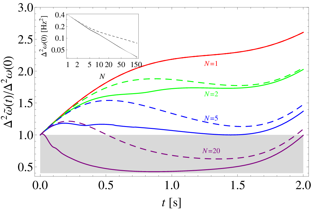
Treating [53] as a guideline we choose $\alpha=1\,\mathrm{Hz}^{2}$, $\gamma=0.2\,\mathrm{Hz}$ so that the OU power spectrum approximates reality for small frequencies $\lesssim 10\mathrm{Hz}$ and set $\beta=10^{-3}\mathrm{Hz}$ to represent the effects of high frequency white noise. The reduction of frequency variance as a function of the interrogation time and the number of atoms used is presented in Fig. 3. We took initial frequency variance $\Delta^{2}\omega(0)=0.167\,\mathrm{Hz}^{2}$ so that the blue solid curve representing the optimal quantum strategy for $N=5$ touches the $\Delta^{2}\omega(t)/\Delta^{2}\omega(0)=1$ line. This indicates that a stationary operation, where the spread due to frequency noise is compensated by estimation feedback, is possible with optimally entangled states of $N=5$ atoms. It is also clear that using product states with the same number of atoms (blue dashed) or a smaller number of entangled atoms does not permit keeping frequency uncertainty at this level. For a given $N$ varying $t$ to minimize $\Delta^{2}\omega(0)$ while keeping the stationary condition fulfilled yields the optimal stationary strategy. The inset depicts the minimal stationary $\Delta^{2}\omega(0)$ as a function of the number of atoms for optimal (solid) and product states (dashed). The clear advantage of quantum over classical strategies is evident. We should also mention that formula (11) allows one to quantify the significance of the prior knowledge in comparison to decoherence effects. Specifically, when $\Delta^{2}\omega(0)\ll\Delta^{2}\omega_{K}(t)$, the prior knowledge is not important and the optimal states are determined solely by the effects of decoherence and will be the same as in the standard QFI approaches [23, 31, 32].

To summarize, we have presented a consistent Bayesian approach to studying the potential quantum enhancement in frequency calibration. The tools presented are general enough to be able to deal with more sophisticated and promising atomic clock setups including many simultaneously evolving atomic ensembles [55, 52]. However, a rigorous connection between our results and the performance of the actual atomic clock, requires the study of the Allan variance, instead of instantaneous variance, as a figure of merit. The Allan variance takes into account the effects of the correlations between subsequent interrogation steps, i.e. $\omega_{LO}(0)$ and $\omega_{LO}(t)-\omega_{LO}(0)$, which is more adequate in the quantification of the performance of atomic clocks but at the same time makes the study of the optimal Bayesian strategies much more involved. We hope to address this problem in the near future. Actually, some work has already been done recently in this direction, using bounds on precision rather than considering optimal estimation strategies [40] or taking a numerical approach based on the semi-definite programming [41].

We thank Wojciech Wasilewski, Jan Kołodyński, Marcin Jarzyna, Andrew Ludlow and Mădălin Guţă for fruitful discussions. This research was supported by the Polish NCBiR under the ERA-NET CHIST-ERA project QUASAR, Foundation for Polish Science TEAM project and the FP7 IP project SIQS co-financed by the Polish Ministry of Science and Higher Education.

References

- [1] Kleppner D 2006 Physics Today 59 10
- [2] Chou C W, Hume D B, Rosenband T and Wineland D J 2010 Science 329 1630–1633
- [3] Hinkley N, Sherman J A, Phillips N B, Schioppo M, Lemke N D, Beloy K, Pizzocaro M, Oates C W and Ludlow A D 2013 Science 341 1215–1218
- [4] Ramsey N F 1980 Physics Today 33 25–30
- [5] Lee H, Kok P and Dowling J P 2002 Journal of Modern Optics 49 2325–2338
- [6] Wineland D J, Bollinger J J, Itano W M, Moore F L and Heinzen D J 1992 Phys. Rev. A 46(11) R6797–R6800
- [7] Holland M J and Burnett K 1993 Phys. Rev. Lett. 71 1355–1358
- [8] Bollinger J J, Itano W M, Wineland D J and Heinzen D J 1996 Phys. Rev. A 54 R4649–R4652
- [9] Berry D W and Wiseman H M 2000 Phys. Rev. Lett. 85 5098–5101
- [10] Giovannetti V, Lloyd S and Maccone L 2006 Phys. Rev. Lett. 96 010401
- [11] Roos C F, Chwalla M, Kim K, Riebe M and Blatt R 2006 Nature 443 316–319
- [12] LIGO Collaboration 2011 Nature Phys. 7 962–965
- [13] Ospelkaus C, Warring U, Colombe Y, Brown K R, Amini J M, Leibfried D and Wineland D J 2011 Nature 476 181–184
- [14] Sewell R J, Koschorreck M, Napolitano M, Dubost B, Behbood N and Mitchell M W 2012 Phys. Rev. Lett. 109(25) 253605
- [15] Caves C M 1981 Phys. Rev. D 23 1693–1708
- [16] Huver S D, Wildfeuer C F and Dowling J P 2008 Phys. Rev. A 78 063828
- [17] Dorner U, Demkowicz-Dobrzański R, Smith B J, Lundeen J S, Wasilewski W, Banaszek K and Walmsley I A 2009 Phys. Rev. Lett. 102 040403
- [18] Demkowicz-Dobrzanski R, Dorner U, Smith B J, Lundeen J S, Wasilewski W, Banaszek K and Walmsley I A 2009 Phys. Rev. A 80(1) 013825
- [19] Knysh S, Smelyanskiy V N and Durkin G A 2011 Phys. Rev. A 83 021804
- [20] Demkowicz-Dobrzański R, Banaszek K and Schnabel R 2013 Phys. Rev. A 88(4) 041802
- [21] Huelga S F, Macchiavello C, Pellizzari T, Ekert A K, Plenio M B and Cirac J I 1997 Phys. Rev. Lett. 79 3865–3868
- [22] Genoni M G, Olivares S and Paris M G A 2011 Phys. Rev. Lett. 106(15) 153603
- [23] Dorner U 2012 New Journal of Physics 14 043011
- [24] Shaji A and Caves C M 2007 Phys. Rev. A 76 032111
- [25] Sarovar M and Milburn G J 2006 J. Phys. A: Math. Gen. 39 8487
- [26] Giovannetti V, Lloyd S and Maccone L 2011 Nature Photon. 5 222–229
- [27] Banaszek K, Demkowicz-Dobrzański R and Walmsley I A 2009 Nature Photon. 3 673–676
- [28] Escher B M, de Matos Filho R L and Davidovich L 2011 Nature Phys. 7 406–411
- [29] Demkowicz-Dobrzański R, Kołodyński J and Guţă M 2012 Nat. Commun. 3 1063
- [30] Kołodyński J and Demkowicz-Dobrzański R 2013 New Journal of Physics 15 073043
- [31] Chin A W, Huelga S F and Plenio M B 2012 Phys. Rev. Lett. 109 233601
- [32] Szankowski P, Chwedenczuk J and Trippenbach M 2012 ArXiv e-prints (Preprint 1212.2528)
- [33] Bužek V, Derka R and Massar S 1999 Phys. Rev. Lett. 82(10) 2207–2210
- [34] André A, Sørensen A S and Lukin M D 2004 Phys. Rev. Lett. 92 230801
- [35] Leibfried D, Barrett M D, Schaetz T, Britton J, Chiaverini J, Itano W M, Jost J D, Langer C and Wineland D J 2004 Science 304 1476–1478
- [36] Mullan M and Knill E 2012 Quantum Info. Comput. 12 553–574 ISSN 1533-7146
- [37] Borregaard J and Sørensen A S 2013 Phys. Rev. Lett. 111(9) 090801
- [38] Helstrom C W 1976 Quantum detection and estimation theory (Academic press)
- [39] Braunstein S L and Caves C M 1994 Phys. Rev. Lett. 72 3439–3443
- [40] Fraas M 2013 ArXiv e-prints (Preprint 1303.6083)
- [41] Mullan M and Knill E 2014 ArXiv e-prints (Preprint 1404.3810)
- [42] Holevo A S 1982 Probabilistic and Statistical Aspects of Quantum Theory (North Holland, Amsterdam)
- [43] Demkowicz-Dobrzański R 2011 Phys. Rev. A 83 061802
- [44] Personick S 1971 Information Theory, IEEE Transactions on 17 240–246 ISSN 0018-9448
- [45] Macieszczak K 2013 ArXiv e-prints (Preprint 1312.1356)
- [46] Jarzyna M and Demkowicz-Dobrzanski R 2014 ArXiv e-prints (Preprint 1407.4805)
- [47] Summy G S and Pegg D T 1990 Opt. Commun. 77 75–79
- [48] Knysh S I, Chen E H and Durkin G A 2014 ArXiv e-prints arXiv:1402.0495
- [49] Monz T, Schindler P, Barreiro J T, Chwalla M, Nigg D, Coish W A, Harlander M, Hänsel W, Hennrich M and Blatt R 2011 Phys. Rev. Lett. 106(13) 130506
- [50] Gross C, Zibold T, Nicklas E, Esteve J and Oberthaler M K 2010 Nature 464 1165–1169
- [51] Numata K, Kemery A and Camp J 2004 Phys. Rev. Lett. 93(25) 250602
- [52] Rosenband T and Leibrandt D R 2013 ArXiv e-prints (Preprint 1303.6357)
- [53] Jiang Y Y, Ludlow A D, Lemke N D, Fox R W, Sherman J A, Ma L S and Oates C W 2011 Nature Photonics 5 158–161
- [54] Domenico G D, Schilt S and Thomann P 2010 Appl. Opt. 49 4801–4807
- [55] Borregaard J and Sørensen A S 2013 ArXiv e-prints (Preprint 1304.5944)
- [56] Hansen F and Pedersen G K 2003 Bulletin of the London Mathematical Society 35 553–564
- [57] Kołodyński J and Demkowicz-Dobrzański R 2010 Phys. Rev. A 82(5) 053804