On stochastic generation of ultrametrics in high-dimensional Euclidean spaces

A set $M=\left\{x\right\}$ is called a metric space if for any pair of elements $x^{a},\,x^{b}\in M$ a distance function $d_{ab}=d(x^{a},x^{b})$ (called a metric) is defined and satisfies the following four axioms for any triplet of points $x^{a},\,x^{b},\,x^{c}$:

A metric $d_{ab}$ satisfying the strong triangle inequality

is called an ultrametric. A space with an ultrametric is called a space with an ultrametric structure or an ultrametric space.

An arbitrary real valued matrix $d=\{d_{ab}\}$ is called a metric matrix if its elements satisfy the conditions (1)–(4), and it is called an ultrametric matrix if its elements satisfy the conditions (1)–(3) and (5).

Classic examples of ultrametric spaces are the field $Q_{p}$ of $p$-adic numbers [1, 2, 3], and the ring $Q_{m}$ of $m$-adic numbers (see, for example, [4]).

Ultrametric spaces had long been used in various fields of natural and social sciences to problems of classification and information processing: optimization theory, taxonomy, cluster and factor analysis, and other [5]. During the last 30 years, the mathematical apparatus of ultrametric analysis was developed by by V.S.Vladimirov and coworkers. This relatively new scientific field of ultrametric mathematical physics is represented by many books and works devoted to development of the $p$-adic analysis, $p$-adic mathematical physics and its application to modeling in various fields of physics, biology, computer science, psychology, sociology, and so on (see [1, 2, 3, 6] and references therein).

In fact a lot of physical, biological or socio-economic systems has intrinsic hierarchical structure [5]. Systems with non–explicit hierarchical structure are of considerable interest to researchers. In such systems the hierarchical structure cannot be observed in the original variables, but it becomes observable after transition to some effective (hidden) variables. Typically the number of these effective variables is essentially smaller than the number of degree of freedom of the whole system. There are reasons to believe that hidden ultrametric structures are present in a number of complex systems (i.e. systems with a large number of heterogeneous interacting objects), which include spin glasses, proteins, nucleic acids, etc. Similar ultrametric models arose in the early eighties last century in statistical physics of spin systems with a disorder [7, 5, 8, 9, 10]. Namely it was found that if the system has large number of "internal contradictions" (frustrations) at different scales, equilibrium of the system can be achieved in hierarchically nested regions of phase space, and number of nesting levels increases with decreasing a temperature. In this case there are relations between phase region scales, that satisfy the strong triangle inequality and thus low-temperature spin states are correlated ultrametrically.

Almost immediately after the appearance of ultrametric spin glass models it has been assumed that the conformational state space of protein molecule has ultrametric structure [11, 12]. In this case states are associated with local minima of the potential energy landscape of a protein molecule, and the energy landscape is represented as a hierarchy of nested basins of free energy local minima. Ultrametric models of conformational dynamics of protein molecules have been developed in a series of papers [13, 14, 15, 16, 17, 18, 19].

There is also some evidence that similar ultrametric structures arise in socio-economic systems [20, 21, 22, 23, 24].

In many cases the idea of application of ultrametric models to complex systems such as proteins came from the theory of spin glasses [11, 12] and there are many arguments in favor of that protein should have the ultrametric structure (see [14] for the discussion of energy landscapes and hierarchical disconnectivity graphs). However, the explanation of the origin of ultrametric structures in spin glasses based on the replica method, which is not quite rigorously justified. Thus it is interesting to discuss alternative approaches to ultrametric structures in complex systems.

In this paper we propose a procedure of generation of ultrametric structure in a metric space. In this procedure we do not assume any ultrametric properties for the initial metric space.

It has been observed in several studies (see, for example, [25, 26]), that the effectiveness of clustering algorithms applied to large data sets significantly increases with increasing the dimension of the array. Moreover it has been observed that the distance between randomly distributed points in multidimensional metric spaces shows ultrametric properties with increasing space dimension. In this paper we give the rigorous proof that any finite ultrametric space can be generated by a special random distribution of points in the $n$-dimensional Euclidean metric space taking the limit $n\rightarrow\infty$. In this case the ultrametric is completely determined by variances of random point coordinates. We present the algorithm for generating such ultrametric spaces. The validity of the algorithm is numerically demonstrated by calculations of distance matrices and ultrametricity indexes for high dimension spaces.

The paper is organized as follows. In Section 2, we present the formulation of our construction. Also in this section we formulate and prove the theorem that is the main result of this article. In Section 3, we describe the algorithm of a stochastic generation of ultrametrics in high-dimensional Euclidean spaces and check the validity of its by numerical simulations.

Let us formulate statements which will be used in our construction.

Let $M=\left\{x^{(a)}\right\},\>a=1,2,\ldots,N$ be a finite ultrametric space with an ultrametric $d\left(x^{(a)},x^{(b)}\right)$. We say that a space $M$ is an isometric space, and an ultrametric $d\left(x^{(a)},x^{(b)}\right)$ is an isometric if for any triplet of points $x^{(a)},\,x^{(b)},\,x^{(c)}$ in $M$ the following condition holds: $d\left(x^{(a)},x^{(b)}\right)=\max\left\{d\left(x^{(a)},x^{(c)}\right),d\left(x^{(b)},x^{(c)}\right)\right\}$, i.e. distances between any two non–coinciding points are equal.

The subset $B_{r}(a)=$ $\left\{x\in M:\>d\left(x,a\right)\leq r\right\}$ is said to be the ball of radius $r$ with the center at the point $a$.

We say that an ultrametric space $M$ is homogeneous, if for any fixed value $r$ of ball radius there is exist the number $m(r)$ such that any ball $B_{r}(a)$ can be represented as a union of $m(r)$ balls of radius $r^{\prime}$, $r^{\prime}<r$.

We say that an ultrametric space $M$ is self-similar, if there exist is the number $m$ such that any ball $B_{r}(a)$ can be represented as a union of $m$ balls of radius $r^{\prime}$, $r^{\prime}<r$.

It is obvious that any self-similar ultrametric space is homogeneous.

A finite self-similar ultrametric space is isomorphic to a boundary of a Cayley tree with a finite number of levels. The distance between points at the boundary of the tree is defined as the weighted length of the path in the tree between these points.

Also we need some statements from probability theory (see, for example, [27, 28, 29]). These results will be used to prove the main result formulated in Theorem 7.

Let $\left\{\Omega,\Sigma,\mathrm{P}\right\}$ be a probability space, where $\left\{\Omega,\Sigma\right\}$ is measurable space, $\mathrm{P}$ is probability measure. Real random variable $X$ is measurable mapping $X:\>\Omega\to R$. For any real random variable $X=X(\omega)$ an interegral $\intop_{A}X\left(\omega\right)d\mathrm{P}\left(\omega\right)$, $A\in\Sigma$ can be defined. An expectation and a variance of $X$ are $\mathsf{E}\left[X\right]=\intop_{\Omega}X\left(\omega\right)d\mathrm{P}\left(\omega\right)$ and $\mathsf{V}\left[X\right]=\mathsf{E}\left[X^{2}\right]-\left(\mathsf{E}\left[X\right]\right)^{2}$ respectively. Let $\Sigma^{(1)}\subset\Sigma$ be a $\sigma$-subalgebra of $\Sigma$, then the conditional expectation $\mathsf{E}\left[X\left|\Sigma^{(1)}\right.\right]$ of real random variable $X$ is a random variable $Y$ that that $Y$ is $\Sigma^{(1)}$ measurable, and for all $A\in\Sigma^{(1)}$ $\intop_{A}X\left(\omega\right)d\mathrm{P}\left(\omega\right)=\intop_{A}Y\left(\omega\right)d\mathrm{P}\left(\omega\right)$, and the conditional variance $\mathsf{V}\left[X\left|\Sigma^{(1)}\right.\right]$ is defined as $\mathsf{V}\left[X\left|\Sigma^{(1)}\right.\right]=\mathsf{E}\left[X^{2}\left|\Sigma^{(1)}\right.\right]-\left(\mathsf{E}\left[X\left|\Sigma^{(1)}\right.\right]\right)^{2}$.

The following theorem is a direct consequence of Theorem 4.

We also have the following theorem.

We state the following generalization of Theorem 6 which can be proved similarly.

The proof Theorem 7 is analogous to the proof of Theorem 6 and is based on the identity

for $k=1,\ldots,N$.

In this section, we describe the procedure for constructing an ultrametric space which is induced by the special random distribution of points in the space $R^{n}$ for high $n$. We restrict ourselves to finite homogeneous ultrametric spaces. Such spaces are equivalent to the boundary of some $N$-level hierarchical tree with fixed numbers of branching $p_{k}$ for every $k$-th level. For $p_{1}=p_{2}=\cdots=p_{N}=p$ the homogeneous ultrametric space is self-similar, and the corresponding hierarchical tree is the $N$-level Cayley tree, with the number of branching equal to $p$. However, following our procedure, one can construct a non–homogeneous finite ultrametric space isomorphic to the boundary of $N$-level hierarchical tree with arbitrary number of branches at each node. The procedure of building such an ultrametric space in accordance with Theorem 7 can be described as follows. We generate $p_{1}$ independent random points $x^{(a_{1})}=\left(x_{1}^{(a_{1})},x_{2}^{(a_{1})},\ldots,x_{n}^{(a_{1})}\right)$ ($a_{1}=1,2,\ldots,p_{1}$ ) in the $n$-dimensional space $R^{n}$ with the normal distribution $\mathcal{N}\left(0,\sigma_{1}\right)$ for each coordinate. Next we generate $p_{1}p_{2}$ independent random points $x^{(a_{1}a_{2})}=\left(x_{1}^{(a_{1}a_{2})},x_{2}^{(a_{1}a_{2})},\ldots,x_{n}^{(a_{1}a_{2})}\right)$ ($a_{1}=1,2,\ldots,p_{1}$, $a_{2}=1,2,\ldots,p_{1}p_{2}$) in $R^{n}$ with normal distribution $\mathcal{N}\left(x_{i}^{(a_{1})},\sigma_{2}\right)$ for $i$-th coordinate. Next we generate $p_{1}p_{2}p_{3}$ independent random points $\left(x_{1}^{(a_{1}a_{2}a_{3})},x_{2}^{(a_{1}a_{2}a_{3})},\right.$$\left.\ldots,x_{n}^{(a_{1}a_{2}a_{3})}\right)$ ($a_{1}=1,2,\ldots,p_{1}$, $a_{2}=1,2,\ldots,p_{1}p_{2}$, $a_{3}=1,2,\ldots,p_{1}p_{2}p_{3}$) in $R^{n}$ with the normal distribution $\mathcal{N}\left(x_{i}^{(a_{1}a_{2})},\sigma_{3}\right)$ for $i$-th coordinate and so on. We repeat this procedure for the generation of random points $N$ times. On the last step we generate $p_{1}p_{2}\cdots p_{N}$ independent random points $x^{(a_{1}a_{2}\cdots a_{N})}=$ $\left(x_{1}^{(a_{1}a_{2}\cdots a_{N})},x_{2}^{(a_{1}a_{2}\cdots a_{N})},\right.$ $\left.\ldots,x_{n}^{(a_{1}a_{2}\cdots a_{N})}\right)$ ($a_{1}=1,2,\ldots,p_{1}$, $a_{2}=1,2,\ldots,p_{1}p_{2}$, $\ldots,$ $a_{N}=1,2,\ldots,p_{1}p_{2}\cdots p_{N}$) in $R^{n}$ with the normal distribution $\mathcal{N}\left(x_{i}^{(a_{1}a_{2}\cdots a_{N-1})},\sigma_{N}\right)$ for $i$-th coordinate. The set of points $M_{n}^{(N)}=\left\{x^{(a_{1}a_{2}\cdots a_{N})}\right\}$ forms the metric space with the metric (10). The metric (10) will converge in probability for $n\to\infty$ to some ultrametric in the sense of Theorem 7.

We introduce some new definitions.

Let $M$ be the finite metric space with elements $x^{(a)}\in R^{n},\>a=1,2,\ldots,N$ and let $d\left(x^{(a)},x^{(b)}\right)$ be the metric on $M$. For for any triplet of points (or for any triangle) $x^{a},\,x^{b},\,x^{c}$ in $M$ we define two functions:

and

where

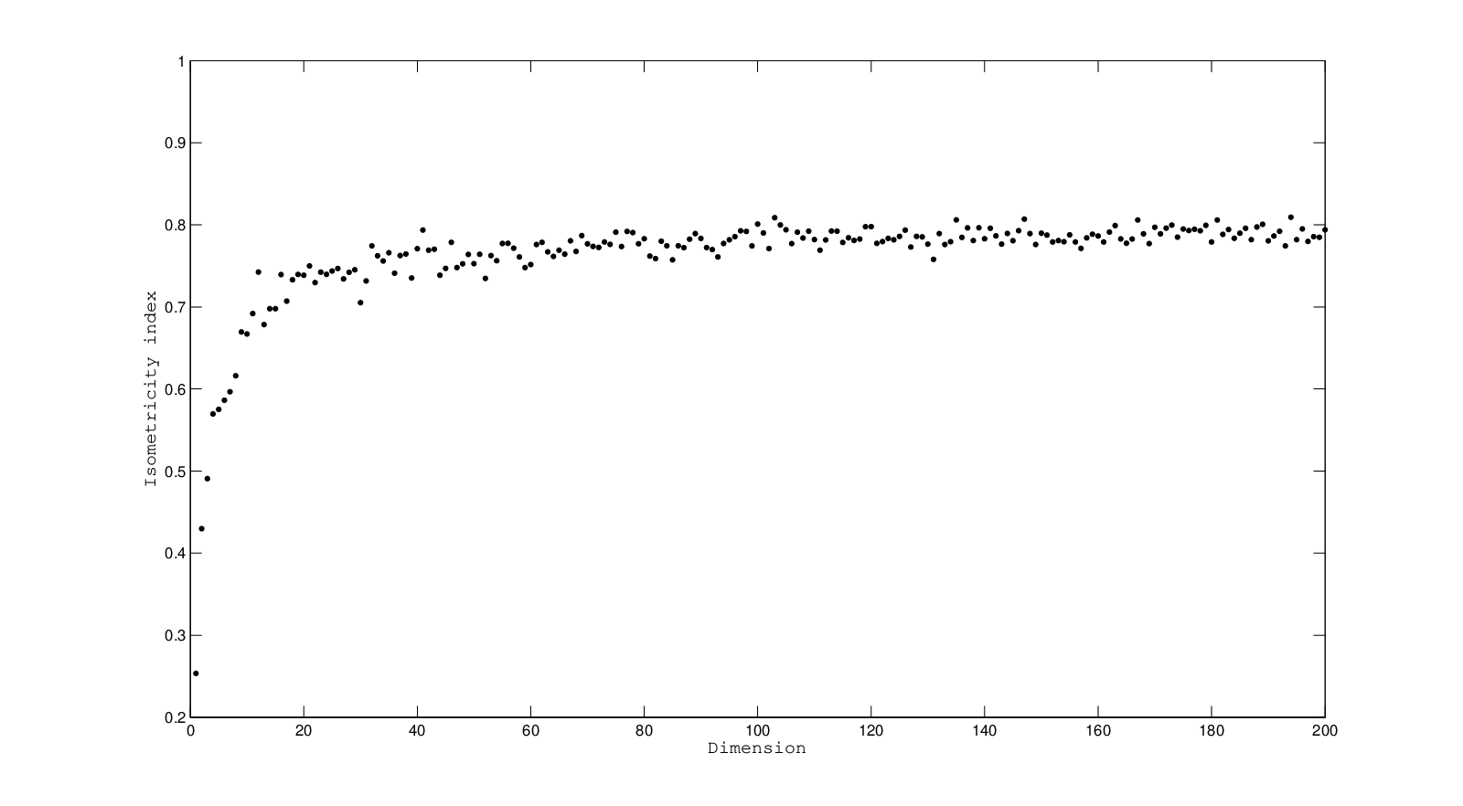
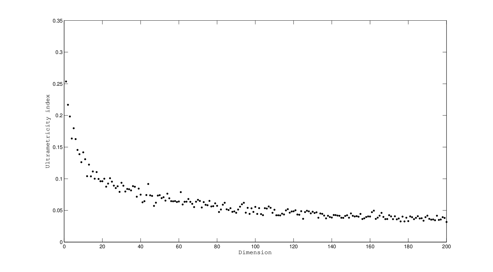
and we call this the middle length of the of the triangle $\left\{x^{(a)},x^{(b)},x^{(c)}\right\}$. We say that $I(a,b,c)$ is the ultrametricity index and $I(a,b,c)$ is the isometricity index of the triangle $\left\{x^{(a)},x^{(b)},x^{(c)}\right\}$.

The ultrametricity index of the metric space $M$ is the number $U\left(M\right)$ defined as the average ultrametricity index of all possible triangles in $M$:

The isometricity index of the metric space $M$ is the number $E\left(M\right)$ defined as the average isometricity index of all possible triangles in $M$:

Note that $0\leq U\left(M\right)\leq\dfrac{1}{2}$, $0\leq E\left(M\right)\leq 1$ and we have $U\left(M\right)=0$ if $M$ is ultrametric and $E\left(M\right)=0$ if $M$ is isometric. It is possible to claim that for metric space $M_{n}^{(N)}$ generated by the procedure described in the previous section

as $n\to\infty$.

Let $d_{n}^{\left(p_{1},p_{2},\dots,p_{N}\right)}\left(N\right)$ be the metric matrix generated numerically according to the above procedure, where $N$ is the number of procedure steps (the level number of the ultrametric tree), $p_{i}$, $i=1,2,\dots,N$ is the numbers of points at the $i$-th step of the procedure. Below we present the metric matrix $d_{n}^{\left(p_{1},p_{2}\right)}\left(2\right)$ and $d_{n}^{\left(p_{1},p_{2},p_{3}\right)}\left(3\right)$. The values of the variances are $\sigma_{1}^{2}=\sigma_{2}^{2}=\sigma_{3}^{2}=1$. The dimension $n$ of the space $R^{n}$ is chosen to be $10^{4}$.

References

• [1] Schikhof W.H. Ultrametric Calculus. An Introduction to pp-adic Analysis, Cambridge Studies in Advanced Mathematics, Cambridge University Press, Cambridge, 1984. viii+306 pp.
• [2] Vladimirov V. S., Volovich I. V., Zelenov E. I., pp-Adic Analysis and Mathematical Physics, Singapure: World Scientific Publishing, 1994, 340 p.
• [3] Albeverio S., Khrennikov A.Yu., Shelkovich V.M., Theory of pp-adic Distributions: Linear and Nonlinear Models, London Mathematical Society Lecture Note Series, 2011, 351 p.
• [4] Dolgopolov M. V., Zubarev A. P., "Some Aspects of mm-Adic Analysis and Its Applications to mm-Adic Stochastic Processes", pp-Adic Numbers, Ultrametric Analysis, and Applications, 3 (2011), N.1, 39–51.
• [5] Rammal R., Toulose G., Virasoro M. A., "Ultrametrisity for physicists", Rev. Mod. Phys., V. 58 (1986), N3., 765–788.
• [6] Dragovich B., Khrennikov A.Yu., Kozyrev S.V., Volovich I.V., "On pp-adic mathematical physics". pp-Adic Numbers, Ultrametric Analysis, and Applications, Vol. 1, No 1, (2009) 1.
• [7] Mezard M., Parisi G., Sourlas N., Toulouse G., Virasoro M.A., "On the nature of the spin-glass phase", Phys. Rev. Lett. 52 (1984) 1156.
• [8] Parisi G., "Infinite number of order parameters for spin-glasses", Phys. Rev. Lett., 43 (1979), 1754–1756.
• [9] Dayson F. J., "Existence of a phase–transition in a one–dimentional Ising ferromagnet", Commun. Math. Phys., 12 (1969), 91–107.
• [10] Dotsenko V, An Introduction to the Spin Glasses and Neural Networks, Singapure: World Scientific, 1994, 159 p.
• [11] Frauenfelder H., "The connection between low-temperature kinetics and life", In Protein Structure, Molecular and Electronic Reactivity, Eds. R. H. Austin et al., Springer, NY, (1987), 245–261.
• [12] Frauenfelder H., "Complexity in proteins", Nature Struct. Biol., V. 2 (1995), 821–823.
• [13] Ogielski A. T., Stein D. L., "Dynamics on ultrametric spaces", Phys. Rev. Lett., V. 55 (1985), 1634–1637.
• [14] Becker O. K., Karplus M., "The topology of multidimentional protein enargy surfaces: theory and application to peptide structure and kinetics", J. Chem. Phys., 106 (1997), 1495–1517.
• [15] Avetisov V. A., Bikulov A. Kh., Kozyrev, S. V., "Application of pp–adic analysis to models of spontaneous breaking of replica symmetry", Journal of Physics A, Vol.32 (1999), 8785–8791.
• [16] Avetisov V. A., Bikulov A. H., Kozyrev S. V, Osipov V. A., "pp-Adic models of ultrametric diffusionh constrained by hierarchical energy landscapes", J. Phys. A: Math. Gen., V. 35 (2002), 177–189.
• [17] Avetisov V. A., Bikulov A. Kh., Osipov V. A., "pp-Adic description of characteristic relaxation in complex systems", J. Phys. A: Math. Gen., 36 (2003), 4239–4246.
• [18] Avetisov, V. A., Bikulov, A. Kh., "Protein ultrametricity and spectral diffusion in deeply frozen proteins", Biophysical Reviews and Letters, 3 (2008) 387–396.
• [19] Avetisov V. A, Bikulov A. H., Zubarev A. P., "First passage time distribution and number of returns for ultrametric random walk", J. Phys. A: Math and Theor., V. 42 (2009), 85005–85021.
• [20] Sornette D., Johansen A., "A hierarchical model of financial crashes", Physica A, V. 261, 1998, P. 581–598.
• [21] Mantenga R.N., Stanley H.E, An Introduction to Econophysics. Correlations and Complexity in Finance, Cambridge Univ. Press, Cambridge, 2000, 147 p.
• [22] Bikulov A.Kh., Zubarev A.P., Kaidalova L.V., "Hierarchic Dynamic Model of Financial Market near Crash Points and pp-adic Mathematical Analysis", Proc. Samara State Tech. Univ., Iss. 42, (2006) 135-141 (in Russian).
• [23] Volov V.T., "Fractal-cluster theory and thermodynamic principles of the control and analysis for the self-organizing systems", arXiv:1309.1415.
• [24] Volov V.T., Zubarev A.P., "Ultrametric dynamics for the closed fractal-cluster resource models", arXiv:1309.4116.
• [25] P. Hall, J.S. Marron and A. Neeman, "Geometric representation of high dimension low sample size data", Journal of the Royal Statistical Society B, 67, 427–444, 2005.
• [26] F. Murtagh, "From data to the physics using ultrametrics: new results in high dimensional data analysis", in B. Dragovich, A. Khrennikov, Z. Rakic and I. Volovich, Eds., Proc. 2nd International Conference on p-Adic Mathematical Physics, American Institute of Physics, 151-161, 2006.
• [27] Durrett R., Probability. Theory and examples, Wadsworth & Brooks/Cole, Pacific Grove, CA, 1991, 453 pp.
• [28] Billingslety P., Probability and measure, New York: Wiley, 1979, xiv+515 pp.
• [29] Shiryaev A.N., Probability, Graduate Texts in Mathematics, 95, Second edition, Springer-Verlag, New York, 1996, xvi+623 pp.
• [30] Slutsky E.E., "Uber Stochastische Asymptoten und Grenzwerte", Metron 5, 1–90.
• [31] Billingsley P., Convergence of Probability Measures, New York, NY: John Wiley & Sons, Inc., 1999, xii+253 pp.