Orthogonal polynomials of equilibrium measures supported on Cantor sets

Iterated Function Systems (IFS) [67, 44, 12, 11, 13, 48] provide a convenient construction of Cantor sets. In the simplest setting, they are collections of contractive maps $\phi_{m}:{\bf R}\rightarrow{\bf R}$, $m=1,\ldots,M$: for any $m$ there exists $\delta_{m}<1$, such that $|\phi_{m}(s)-\phi_{m}(t)|\leq\delta_{m}|s-t|$. There exists a unique set $E$, called the attractor of the IFS, that solves the equation

In the above, we have also defined the operator $\Phi$, acting on the set of compact subsets of ${\bf R}$. This space is complete in the Hausdorff metric, and $\Phi$ is there contractive. Therefore, the attractor $E$ is also the limit of the sequence $\Phi^{n}(E_{0})$, where $E_{0}$ is any non-empty compact set: $E=\lim_{n\to\infty}\Phi^{n}(E_{0}).$

The set of measures supported on $E$ is rich and wide. We will restrict our consideration to two kinds of measures of mathematical and physical significance: equilibrium measures and balanced measures. The former having been defined in the Introduction, let us now describe the latter. They are obtained associating a probability, or weight, $\pi_{m}>0$, $m=1,\ldots,M$, to each IFS map: $\sum_{m}\pi_{m}=1$. For any such choice of weights, a unique positive measure $\mu$ on $E$ satisfies the equation

for any continuous function $f$. For instance, consider the set of one–dimensional affine maps of the form:

where $\delta_{m}$ are real numbers between zero and one, called contraction ratios, and $\gamma_{m}$ are real constants, the fixed points of the maps. Under these conditions, the attractor $E$ is a finite or infinite collection of intervals, or a Cantor set [62, 63].

Equation (8) can be rewritten as $\int fd\mu=\int(Tf)d\mu$, where we have introduced the transfer operator $T$. By going to the dual space of Borel probability measures, ${\cal M}$, this equation is equivalent to $T^{*}\mu=\mu,$ where $T^{*}$ is the adjoint operator of $T$, also known as the Perron–Frobenius operator. This operator is contractive in the Hutchinson–Wesserstein metrics, so that the sequence of discrete measures $\mu_{n}:=(T^{*})^{n}\mu_{0}$, for any $\mu_{0}$, converges in the complete space ${\cal M}$. This permits to define a first sequence of discrete measures. As above, let $D_{x}$ be the Dirac measure located at the point $x$.

A second interesting family of I.F.S. maps consists of the real inverse roots of polynomials in a complex variable.

Observe that the two maps in eq. (11) are the inverse branches of the quadratic transformation $z\rightarrow z^{2}-\lambda$, so that the IFS attractor $E$ is the Julia set of this map. When $\lambda=2$ this set is the interval $[-2,2]$ and the balanced measure is the Chebyshev measure, i.e. the equilibrium measure on $E$: $\mu=\nu_{E}$. This remarkable coincidence is general:

For proof and theory of Julia sets see [49, 30, 19, 17]. Out of this beautiful theory we need to recall a second fact: because of the renormalization relation $p_{2j}(\nu_{E};\phi_{\pm}(x))=p_{j}(\nu_{E};x)$, the Jacobi matrix $J(\nu_{E})$ can be computed via simple recursions [15, 14], $a_{j}=0$ for all $j$, while $b_{1}=\lambda$, $b_{2j}=b_{j}/b_{2j-1}$ and $b_{2j+1}=\lambda-b_{2j}$. We will use these relations in Sect. 7.

The logarithmic capacity of the attractor $E$ of an IFS has been studied in [10, 75, 64]. We now compute numerically its equilibrium measure, following [64]. Let $E_{0}$ be the convex hull of $E$, that can be easily be identified as the interval $E_{0}=[\gamma_{1},\gamma_{M}]$, where we have ordered the IFS maps according to increasing values of their fixed points: $\gamma_{j}<\gamma_{j+1}$, for any $j=1,\ldots,M-1$. The set $E$ is the limit, in the Hausdorff metric, of the sequence of compact sets $E_{n}:=\Phi^{n}(E_{0})$, see eq. (7), each of which the union of $N$ disjoint, closed intervals $E_{n}^{i}$:

The maximum cardinality, $N=M^{n}$, is met in the case of fully disconnected IFS, (i.e. those for which the intervals $\{\phi_{m}(E_{0})\}_{m=1}^{M}$ are pairwise disjoint). We denote the intervals in eq. (12) as $E_{n}^{i}:=[\alpha_{i},\beta_{i}]$, dropping for simplicity the generation index $n$ when confusion cannot occur. The idea of approximating $E$ by the nested sequence of sets $E_{n}$ has proven to be useful also theoretically [4]: thanks to basic properties of the logarithmic potential, capacity and Green’s function can be continuously obtained in the limit $n\rightarrow\infty$. The same holds for equilibrium measures and Jacobi matrices, as we will see momentarily.

The equilibrium problem for a finite union of $N$ intervals $[\alpha_{i},\beta_{i}]$, $i=1,\ldots,N$, has a well known analytical solution [3, 90, 68, 54, 7, 69, 70, 71, 20]: define the polynomial $Y(z)$,

and its square root, $\sqrt{Y(z)}$, as the one which takes real values for $z$ real and large. Also, let the real numbers $\xi_{i}$ belong to the open intervals $(\beta_{i},\alpha_{i+1})$, for $i=1,\ldots,N-1$. Define $Z(\xi;z)$ as the monic polynomial of degree $N-1$ with roots at all $\xi_{i}$’s:

Then, there exists a unique set of values $\{\zeta_{i}\}_{i=1,\ldots,N-1}$ that solve the set of coupled, non–linear equations

A stable technique for the solution of the non-linear equations (15) has been presented in [64]. To reduce its memory and computer time requirements we developed a different technique, that is described in Appendix A, not to interrupt here the natural flow of arguments.

When the solution $\{\zeta_{i}\}_{i=1,\ldots,N-1}$ of equations (15) is known, the equilibrium measure on $E_{n}$, denoted by $\nu_{n}:=\nu_{E_{n}}$, can be computed as the absolutely continuous measure (with respect to the Lebesque measure on $E_{n}$), consisting of the sum of $N$ measures supported on each of the $N$ intervals $E_{n}^{i}$:

The properties of the orthogonal polynomials of $\nu_{n}$, and of the Green’s function of $E_{n}$ have been studied in [3, 90, 68, 7, 69, 70, 36]. In particular, the algebraic approach of [71, 54, 55] can be turned into a symbolic computation of these quantities. In this paper, to the contrary, we adopt a numerical strategy.

In fact, when considering the $i$-th interval composing $E_{n}$, the function $Y(s)$ can be factored as $Y(s)=(s-\alpha_{i})(\beta_{i}-s)\tilde{Y_{i}}(s)$, with obvious meaning of the function $\tilde{Y}_{i}(s)$. Therefore, the measure with density $\frac{|Z(\zeta;s)|}{\pi\sqrt{|Y(s)|}}$ with respect to the Lebesgue measure on $[\alpha_{i},\beta_{i}]$, can also be seen as the absolutely continuous measure, with respect to the Chebyshev measure on the same interval, with density $\frac{|Z(\zeta;s)|}{\sqrt{|\tilde{Y}_{i}(s)|}}$:

This fact enables us to define a second sequence of point measures:

In Figure 1 we plot $\Omega_{n}^{G}(x):=\int_{\alpha_{1}}^{x}d\nu_{n}^{G}$, the distribution function of the discrete measure $\nu_{n}^{G}$, versus $x$, for $n=1,\ldots,5$, when $G$ is kept constant and large, in the case of Example 1. Since $\nu_{n}$ tends to the equilibrium measure $\nu_{E}$ on $E$ when $n$ tends to infinity, it is clear that letting both $n$ and $G$ grow simultaneously²² 2 One can also choose a different number of Gaussian points for each set $E_{n}^{i}$. This is useful when their lengths are vastly different, like in affine IFS with different contraction ratios, or in the Julia set case. we can devise a sequence of discrete measures $\nu_{n}^{G}$ converging to $\nu_{E}$. An efficient procedure to rule their combined increase can be derived by the convergence of the corresponding Jacobi matrix entries, as we will show in Sect. 7.

Finally, observe that the distribution of atoms composing $\nu^{G}_{n}$ is not a proper Gaussian measure associated with $\nu_{n}$ (one that is obtained by diagonalization of a truncation of the Jacobi matrix—see below, in Sect. 4); rather, it is a more easily computable approximation, in the same spirit of near–optimal distributions of Riesz energy points on manifolds [41].

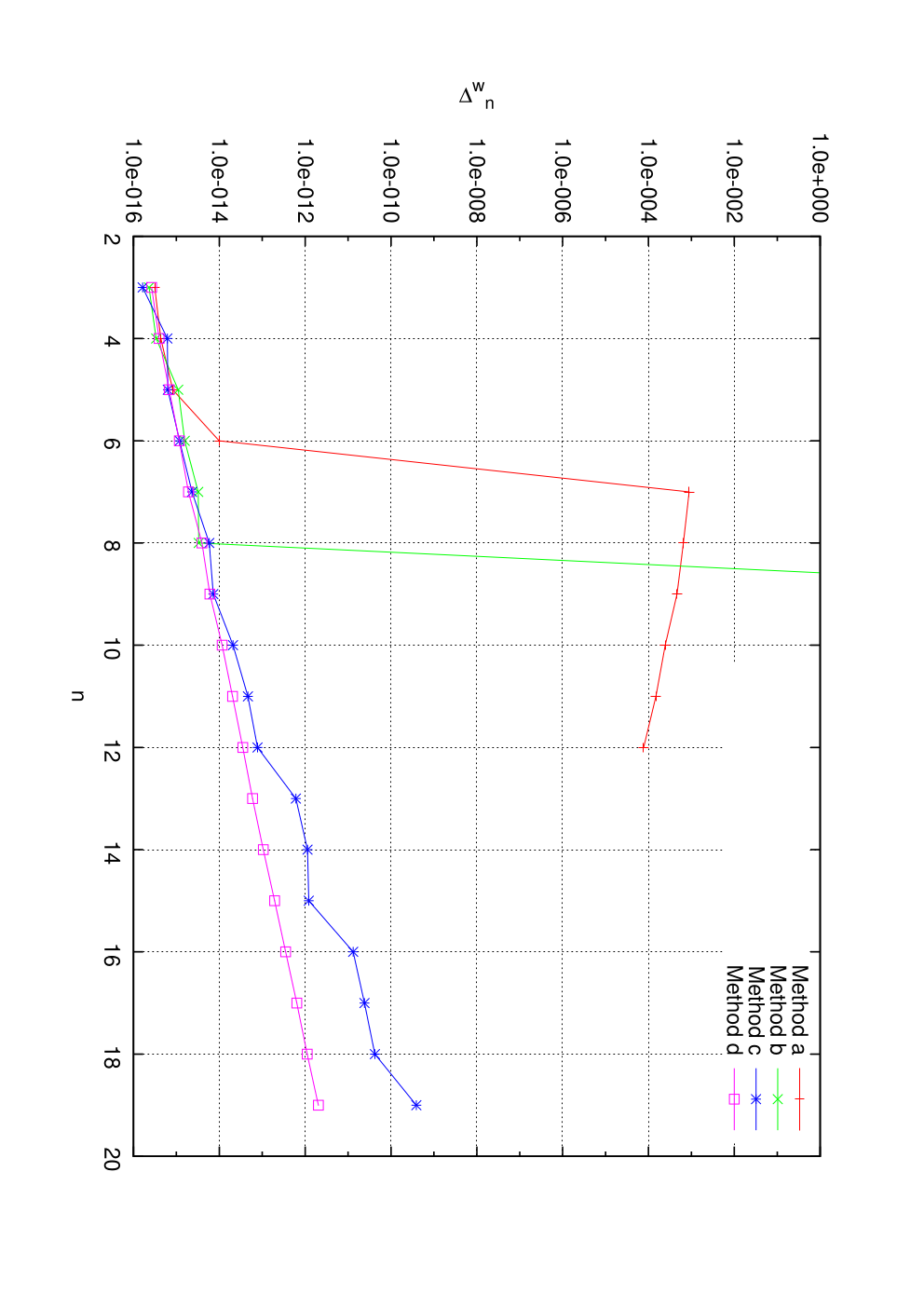
In the previous sections we have described two sequences of discrete measures, $\{\mu_{n}\}_{n\in{\bf N}}$ (eq. 10) and $\{\nu_{n}^{G}\}_{G\in{\bf N}}$ (eq. 18) that converge to $\mu$ and $\nu_{n}$, respectively. Algorithms to compute the Jacobi matrix of discrete measures number in the many. Yet, when applied to sets of atoms of large cardinality, whose locations approach a Cantor set, they may suffer from numerical instabilities. Therefore, in this section we test four algorithms, in search for the best to be applied to our problem. They are: a: an implementation of the Stieltjes/Lanczos technique, where integration is performed by a finite summation; b: Fischer’s approach [32] of adding an atomic measure to a second measure (known via its Jacobi matrix); c: Laurie’s quotient-difference method [52]; d: Gragg and Harrod’s algorithm RKPW [39], based on plane rotations.

Numerical experiment 1. Consider the weakly convergent sequence $\{\mu_{n}\}_{n\in{\bf N}}$, Sequence 1, in the case of Example 1. For each $n$, compute the associated Jacobi matrix $J(\mu_{n})$, of size $N=M^{n}$, (here, $M=2$) via each of the four algorithms above. Next, diagonalize this latter:

to obtain, via the Golub–Welsh algorithm [38], eigenvalues $\lambda_{i}$ and squared first components of the normalized eigenvectors, $v_{i}=(e_{0},{\bf u}_{i})^{2}$, for $i=1,\ldots,N$.

The last set of values should exactly reproduce the points and weights, $x_{i}$ and $w_{i}$, respectively, defining the discrete measure $\mu_{n}$. The $L^{1}$ errors in this reconstruction are $\Delta^{x}_{n}:=1/N\sum_{i}|x_{i}-\lambda_{i}|$ and $\Delta^{w}_{n}:=1/N\sum_{i}|w_{i}-v_{i}|$. In Figure 2 we plot $\Delta^{w}_{n}$ versus $n$, for the four methods listed above. The errors $\Delta^{x}_{n}$ are smaller than $\Delta^{w}_{n}$ and are not plotted. We observe that the Lanczos technique gives fully unreliable results at $n=7$, while Fischer’s method breaks down (negativity of a positive definite quantity) at $n=9$. To the contrary, methods c and d never break down in the range explored. Method d seems to be the best, featuring an error that increases as a power–law in $N$, with exponent smaller than one. Since the results of this experiment are typical, we have adopted Gragg and Harrod’s algorithm (RKPW henceforth) in the computations of this paper. In Appendix B we show that it can be conveniently programmed on a parallel computer, and that its computational complexity can be significantly reduced, when considering finite Jacobi matrices of rank much less than the number of atoms in the associated measure.

In the previous section we have computed the Jacobi matrices of the measures $\{\mu_{n}\}_{n\in{\bf N}}$, that converge to the balanced measure $\mu$ of an IFS. This provides a new algorithm for the difficult numerical problem of computing the Jacobi matrix $J(\mu)$. Since this latter can also be obtained by different, non iterative techniques [31, 56, 65], we can measure the convergence of the matrix entries of $J(\mu_{n})$ as a function of the order $n$, to assess the relative performance the new algorithm. For this, we further analyze the results of Experiment 1.

Because of symmetry, diagonal Jacobi entries are constant and equal within numerical precision for both $\mu$ and $\mu_{n}$, permitting us to focus on outdiagonal ones, denoted by $b_{l}$ and $b^{n}_{l}$, respectively. In Figure 3 we plot $\Delta^{b}_{n,j}$, the average difference between the first $j+1$ entries of $J(\mu)$ and $J(\mu_{n})$:

In the figure, drawn in doubly logarithmic scale, we observe a region where curves are approximately linear and parallel. In this range, at fixed $j$, the difference between the Jacobi matrix entry of $\mu$ and that of $\mu_{n}$ vanishes exponentially fast in $n$, until it attains machine precision. This region extends unlimitedly (within the reach of these experiments) to large values of $j$: this experimental manifestation of stability proves that the procedure of the previous section defines an algorithm to compute the Jacobi matrices of balanced IFS measures.

Let us now examine quantitatively the performance of this algorithm, by considering the absolute error in the computation of $J(\mu)$. Let us fix a threshold $\epsilon$ and let us find the rank of the largest truncation of $J(\mu)$, that is approximated within $\epsilon$ by $J(\mu_{n})$. We call this rank $N_{\epsilon}(n)$. It can be formally defined via a quantity that will be repeatedly used in the following: the $\epsilon$–coincidence range, $\Lambda_{\epsilon}(J,J^{\prime})$, of two Jacobi matrices $J$ (with entries $a_{j},b_{j})$ and $J^{\prime}$ (with entries $a^{\prime}_{j},b^{\prime}_{j})$ is the integer number

Using this quantity, we can write that $N_{\epsilon}(n)=\Lambda_{\epsilon}(J(\mu),J(\mu_{n}))$. Letting the threshold take the value $\epsilon=10^{-8}$ yields the values reported in Table 1. Since the number of atoms in $\mu_{n}$ is $N=2^{n}$, these data can be well described by a power–law of the kind $N_{\epsilon}\sim A(\epsilon)N^{\beta}$, where $\beta$ can be estimated as $\beta\simeq.912$. Let us now go back to Figure 3, where $N_{\epsilon}(n)$ is approximately the abscissa of the intersection of the plotted curves with an horizontal line at ordinate $\epsilon$. In the linear range in Fig. 3, one also finds that $A(\epsilon)\sim C\epsilon^{\eta}$, with $\eta\simeq.286$ and $C$ a quantity independent of $\epsilon$ and $n$. Taking into account that the computational complexity of the revised RKPW algorithm is approximately of $BN_{\epsilon}N$ arithmetical operations (with $B$ a small constant, see Appendix B), we can conclude that estimating the Jacobi matrix of $\mu$ of size $N_{\epsilon}$ within $\epsilon$ via this procedure has a cost that scales roughly as $\epsilon^{-\eta/\beta}N_{\epsilon}^{1+1/\beta}\simeq\epsilon^{-.31}N_{\epsilon}^{2.09}$, that is, slightly more than quadratic in the size $N_{\epsilon}$ and slowly increasing with respect to the precision $1/\epsilon$. Remark that the recursive algorithms for IFS with a finite number of maps [56, 65] require an order of $N_{\epsilon}^{2}$ operations to compute the same matrix, but this computation is exact in principle, in practice affected by a slowly increasing error [65]. The new algorithm ³³ 3 Notice that in this section the computation of the effective size $N_{\epsilon}(n)$ has been effected a posteriori, using an independent knowledge of the Jacobi matrix of $\mu$. A simple technique to overcome this difficulty can be devised, mimicking Algorithm 1 of the next section. To keep the presentation contained, we do not lay down explicitly these steps, that compose Algorithm 0 in this paper. is therefore not optimal for balanced measures, but it can be extended to equilibrium ones, for which no alternative techniques are available, except for an algebraic procedure that can be set up using a Padé scheme [55].

The techniques of the previous two sections can also be applied to the double–index sequence of measures $\nu_{n}^{G}$. When the order $n$ is kept fixed and $G$ tends to infinity, $\nu_{n}^{G}$ tends weakly to $\nu_{n}$, the equilibrium measure on $E_{n}$, and its Jacobi matrix tends to $J(\nu_{n})$: numerically, this problem is interesting in itself, and we want to investigate the nature of this convergence. We set up the following algorithm:

• Algorithm 1. Computing the Jacobi matrix $J(\nu_{n})$.
  Input: The number of Gaussian points $G$, the threshold $\epsilon$, the IFS parameters, the order $n$ of the IFS construction and a small positive integer $g$.
  Output: the (truncated) Jacobi matrix $J(\nu_{n})$, of rank $N_{\epsilon}(n,G)$ and absolute component-wise error less than $\epsilon$.

• 1:

  Compute points and weights for $\nu_{n}^{G}$, eq. (18), solving the non-linear system of eqs. (15), as described in ref. [64] and in Appendix A.

• 2:

  Compute $J(\nu_{n}^{G})$ via the revised RKPW algorithm, Appendix B.

• 3:

  Decrease $G$ by the amount $g$ and redo steps [1] and [2].

• 4:

  Compute $N_{\epsilon}(n,G):=\Lambda_{\epsilon}(J(\nu_{n}^{G}),J(\nu_{n}^{G-g}))$ as in eq. (21).

A few remarks are in order. The above algorithm works for any finite set of intervals, and not only for IFS intervals. The cardinality of the atoms of $\nu^{n}_{G}$ is $G\times M^{n}$: a set of $G$ Gaussian points is used for each interval $E_{n}^{j}$, $j=1,\ldots,M^{n}$. This number is typically much larger than $N_{\epsilon}(n,G)$, so that the improvement of the RKPW algorithm presented in Appendix B becomes crucial. Finally, the quantity $N_{\epsilon}(n,G)$ is a numerical estimate of the true approximation range $\Lambda_{\epsilon}(J(\nu_{n}^{G}),J(\nu_{n}))$. Using this quantity we will say that the Jacobi matrix $J(\nu_{n})$ of size $N_{\epsilon}(n,G)$ has been effectively computed within $\epsilon$. We start now by testing the performance of this algorithm in the Julia set example described above.

Numerical experiment 2. Consider the IFS in Example 2 with $\lambda=2.1$ and apply algorithm 1 with $g=1$.

In Figure 4 we plot the rank of the effectively computed Jacobi matrix, $N_{\epsilon}(n,G)$, as a function of the total number of Gaussian points, $G\times 2^{n}$. Data for $n=3,4,5$ and $\epsilon=10^{-12}$ show a similar linear behavior, $N_{\epsilon}(n,G)\sim A\;G\times 2^{n}$. The slope $A$ of these linear laws varies little from one case to the next, with a slightly decreasing trend. For instance, data for $n=3$ can be fitted by $A\simeq.675$, while the slope for the case $n=5$ is $A\simeq.647$. In addition, in Figure 4 we have also plotted data for $n=3$, $\epsilon=10^{-2}$: they lie approximately on a line of slope $A\simeq.725$.

Consider now a horizontal line in the plot, going from left to right at fixed ordinate, say $N_{\epsilon}=H$. This line encounters the data for $n=3$, $\epsilon=10^{-2}$, at a certain value of the abscissa. This is the number of Gaussian points required to compute the truncated Jacobi matrix $J(\nu_{n})$, of rank $H$, within maximum component-wise error $\epsilon$. Still moving to the right, one rapidly encounters the data for $n=3$, $\epsilon=10^{-12}$, at a new value of the abscissa. In the segment between these two points of intersection the error decreases by orders of magnitude—quickly reaching the maximum precision attainable.

Indeed, in Algorithm 1 we cannot set a threshold $\epsilon$ smaller than what allowed by the algorithm and the machine on which it is implemented. The point at which the algorithm hits the maximum precision can be found by the break-up of the increase of the approximation range, $N_{\epsilon}(n,G)$.

Numerical experiment 3. Compute, in the same case of Experiment 2, the number of Gaussian points $\tilde{G}$ at which a further increase of $G$ does not lead to an increase of the approximation range $N_{\epsilon}(n,G)$.

Using the value $\tilde{G}$ we can find the maximum rank reachable by the algorithm, $N^{up}(\epsilon,n)=N_{\epsilon}(n,\tilde{G})$. In Figure 5 we plot this quantity versus $\epsilon$, for $n=3$ and $n=10$. No effort was made to have particularly clean data, since our goal here is just to estimate the law of error growth. Both sets of data are consistent with a linear dependence of $N^{up}(\epsilon,n)$ with $\epsilon$. This fact can be turned around, to imply that the minimal numerical error in the determination of the $j$-th line of the Jacobi matrix $\{(a_{j}$, $b_{j})\}_{j\in\bf N}$ grows linearly with $j$, when running Algorithm 1. We deem this to be an optimal result.

We are now equipped with the building blocks to compute the Jacobi matrix $J(\nu_{E}$), the main goal of this work. We will combine the theory of Sect. 3 with the numerical techniques of Sect. 4 and 6. Our approach is to increase alternatively the two indices of $\nu_{n}^{G}$. This is implemented in the following algorithm:

• Algorithm 2. Computing the Jacobi matrix $J(\nu_{E})$.
  Input: The IFS parameters, the maximum order $\bar{n}$, the initial number of Gaussian points $G_{0}$, the threshold $\epsilon$, an increase ratio $\eta>1$.
  Output: the (truncated) Jacobi matrix $J(\nu_{E})$, of rank $H(\epsilon,\nu_{E})$ and absolute component-wise error less than $\epsilon$.

• 1:

  Let $n=2$, $G=G_{0}$

• 2:

  Compute the truncated Jacobi matrix $J(\nu_{n-1}^{MG})$ and its effective size at approximation $\epsilon$, $N_{\epsilon}(n-1,MG)$, via Algorithm 1.

• 3:

  Similarly, compute the truncated Jacobi matrix $J(\nu_{n}^{G})$, and $N_{\epsilon}(n,G)$. Let $N=\min(N_{\epsilon}(n-1,MG),N_{\epsilon}(n,G))$.

• 4:

  Compute $H_{\epsilon}(n)=\Lambda_{\epsilon}(J(\nu_{n-1}^{MG}),J(\nu_{n}^{G}))$.

• 6:

  If $H_{\epsilon}(n)$ is equal to $N$, increase $G$ to $\eta G$ (or to $G+1$ when this is larger) and loop back to step 2. Otherwise continue.

• 7:

  If $n$ is smaller than $\bar{n}$ increase $n$ by one and loop back to step 2. Otherwise stop, since the truncated Jacobi matrix $J(\nu_{\bar{n}}^{G})$ of size $H(\epsilon,\nu_{E})=H_{\epsilon}(\bar{n})$ is an $\epsilon$–approximation of $J(\nu_{E})$.

For any $n$, starting from the lowest, this algorithm computes finite truncations of $J(\nu_{n})$ and $J(\nu_{n-1})$, accurate within a threshold $\epsilon$, with $G$ and $MG$ Gaussian points, respectively (recall that $M$ is the number of IFS maps). While comparing these matrices component–wise, it raises $G$ in order to find the maximum rank in which they coincide, again within the threshold $\epsilon$. This rank naturally increases with the order $n$. We now investigate the performance of this algorithm in the two examples described above.

It is well known that balanced and equilibrium measures on the ternary Cantor set $E$, as well as the finite sets of intervals $E_{n}$, are regular, in the sense described in [81]. Let $\sigma$ be any of these measures, and let $\nu$ be the measure $\nu_{E}$ or $\nu_{n}$, accordingly. Since these sets have positive capacity, empty interior and connected complement, regularity means that the limit (3) exists, and is equal to the equilibrium measure on $E$ (regularity of the zero distribution) and that, equivalently, the limit of $\log|p_{j}(\sigma;z)|^{1/j}$ is the Green’s function ${g(E;z)}$, (or ${g(E_{n};z)}$, in the finite $n$ case), defined in eq. (6), locally uniformly outside the convex hull of $E$ (regular $j$-th root asymptotic behavior): see thms 3.1.1 and 3.1.4 in [81]. The last relation involves the modulus of the orthogonal polynomials. It is easy to extend the j-th root behavior to the complex monic⁴⁴ 4 i.e those for which the coefficient of $z^{j}$ is one, used here for simplicity. Recall that these polynomials satisfy the recursion relation $P_{j+1}(\sigma;z)=(z-a_{j})P_{j}(\sigma;z)-b_{j}^{2}P_{j-1}(\sigma;z)$. orthogonal polynomials $P_{j}(\sigma;z)$.

Since $P_{j}(\sigma;z)=\prod_{l=1,\ldots,j}(z-\xi^{j}_{l})$, regularity of the zero distribution implies that the following limit exists:

with the principal determination of the logarithm, when $z$ does not belong to the support of $\sigma$. The integral in the above equation defines the complex potential $\Psi(\nu;z)$. Its real part is the electrostatic potential, $V(\nu;z)$, eq. (4), so that the real part of eq. (22) conveys the conventional meaning of regular root asymptotics. In the finite $n$ case, the function $\Psi(\nu_{n};z)$, is the same as the complex Green’s function of Widom ([90] eq. 14.1), modulo the constant $\log(\mbox{Cap}(E_{n}))$:

Introducing the polynomial ratios $\rho_{j}(\sigma;z):=P_{j}(\sigma;z)/P_{j-1}(\sigma;z)$ in eq. (22) and taking real and imaginary parts leads to:

and

This procedure reveals the nature of a Lyapunov exponent [46, 47] for the real part of the complex potential, eq. (24); it also makes clear that weaker requirements are needed for root asymptotics, with respect to ratio asymptotics—this latter being the existence of the limit of $\rho_{j}$ [81, 53].

Let us now come to the imaginary part, eq. (25). The arguments in this equation are assumed to lie in the interval $(0,2\pi)$. When $z=x+iy$ tends to the real axis from the above, the left hand side of this equation becomes the conventional rotation number of the theory of discrete Sturm–Liouville operators [26, 46]. Coherently, in this limit the right hand side $\Im\Psi(\nu;z)$ tends to $-\pi\nu([x,\infty))$. Therefore, the imaginary part of the complex potential $\Psi(\nu;z)$ extends the rotation number to the complex plane [46] and the left hand side of eq. (25) gives a practical means to compute it.

We want now to investigate the numerical implications of eqs. (24,25). The function $\Psi(\nu;z)$ is an integral with respect to $\nu$, eq. (22), that can be numerically estimated by a limit procedure, quite analogous to that of Sects. 6,7, of the corresponding integrals with the discrete measures $\nu_{n}^{G}$. Moreover, using the Jacobi matrices of $\nu_{n}$ and $\nu_{E}$, we can also compute the left hand side of eqs. (24,25) and verify experimentally the rate at which convergence takes place in root asymptotics.

Numerical experiment 6. In the case of Example 1, Experiment 5, choose $\sigma=\nu_{n}$ and compute the sequence of real parts $g_{n,j}(z):=\log(|P_{j}(\nu_{n};z)|)/{j}$ using the recursion relation $\rho_{i+1}=(z-a_{i})\rho_{i}-b_{i}^{2}/\rho_{i-1}$ for the left hand side of eq. (24). Using the discrete measures $\nu_{n}^{G}$ in the integral (22), also compute the potential $V(\nu_{n};z)$.

References

- [1] N.I. Akhiezer, The Classical Moment Problem, Hafner, New York, NY. (1965).
- [2] N. I. Akhieser, General theory of the P. L. Tchebycheff polynomials. Translated from the 1945 Russian original by B. Bojanov and G. Nikolov, East J. Approx. 12, 211–259 (2006).
- [3] N. I. Akhieser, Orthogonal polynomials on several intervals, Dokl. Akad. Nauk SSSR 134 9–12 (1960) (Russian); translated as Soviet Math. Dokl. 1 989–992 (1960)
- [4] V.V. Andrievskii, Constructive function theory on sets of the complex plane through potential theory and geometric function theory, Surveys in Approximation Theory, 2 1-52 (2006)
- [5] V.V. Andrievskii, On the Green function for a complement of a finite number of real intervals, Constr. Approx. 20 565–583 (2004).
- [6] V.V. Andrievskii, The highest smoothness of the Green function implies the highest density of a set, Ark. Mat. 42 217–238 (2004).
- [7] A.I. Aptekarev, Asymptotic properties of polynomials orthogonal on a system of contours, and periodic motion of Toda lattices, Math. USSR Sb. 53 (1986) 233–260.
- [8] J. Avron, B. Simon, Almost periodic Schrödinger operators. II. The integrated density of states, Duke Math. J. 50 (1983) 369–39.
- [9] G.A. Baker, D. Bessis, P. Moussa, A family of almost periodic Schrödinger operators, Phys. A 124 61–77 (1984).
- [10] L. Baribeau, D. Brunet, T. Ransford and J. Rostand, Iterated function systems, capacity and Green’s functions, Comput. Methods Funct. Theory 4 (2004) 47–58.
- [11] M. F. Barnsley, Fractals Everywhere, Academic Press, New York, NY (1988).
- [12] M. F. Barnsley and S. G. Demko, Iterated function systems and the global construction of fractals, Proc. R. Soc. London A 399 (1985) 243–275.
- [13] M.F. Barnsley, J. Elton, D.P. Hardin, Recurrent iterated function systems. Fractal approximation, Constr. Approx. 5 3–31 (1989).
- [14] M. F. Barnsley, J. S. Geronimo and A. N. Harrington, Almost periodic Jacobi matrices associated with Julia sets for polynomials, Comm. Math. Phys. 99 303–317 (1985).
- [15] J. Bellissard, D. Bessis, and P. Moussa, Chaotic states of almost–periodic Schrödinger operators, Phys. Rev. Lett. 49 701–704 (1982).
- [16] J. Bellissard, R. Lima, D. Testard, Almost periodic Schrödinger operators, in Mathematics + Physics 1, 1–64, World Sci. Publishing, Singapore, (1985).
- [17] D. Bessis, J. Geronimo, and P. Moussa, Mellin transforms associated with Julia sets and physical applications, J. Stat. Phys. 34 75–110 (1983).
- [18] C. Brezinski, M. Redivo Zaglia, Extrapolation Methods: Theory and Practice, North Holland, Amsterdam (1991).
- [19] H. Brolin, Invariant sets under iterations of rational functions, Ark. Mat. 6 103-144 (1965).
- [20] J. S. Christiansen, B. Simon, M. Zinchenko, Finite gap Jacobi matrices, I. The isospectral torus, Constr. Approx. 32, 1–65 (2010).
- [21] J. S. Christiansen, B. Simon, M. Zinchenko, Finite gap Jacobi matrices, III. Beyond the Szegö class, Constr. Approx. 35 259–272 (2012).
- [22] J. S. Christiansen, Szegö’s theorem on Parreau-Widom sets, Adv. Math. 229 1180–1204 (2012).
- [23] H.L. Cycon, R.G. Froese, W. Kirsch, B. Simon, Schrödinger operators with application to quantum mechanics and global geometry, Springer-Verlag, Berlin (1987).
- [24] D. Damanik, A. Gorodetski, Spectral and quantum dynamical properties of the weakly coupled Fibonacci Hamiltonian, Comm. Math. Phys. 305 221–277 (2011).
- [25] D. Damanik, B. Simon, Jost function and Jost solution for Jacobi matrices, I, Invent. Math. 165, 1–50 (2006).
- [26] F. Delyon and B. Souillard, The rotation number for finite difference operators and its properties, Comm. Math. Phys. 89, 415–426 (1983).
- [27] E. Diekema, T.H. Koornwinder, Differentiation by integration using orthogonal polynomials, a survey, J. Approx. Theory 164, 637-667 (2012).
- [28] T.A. Driscoll, L. N. Trefethen, Schwarz-Christoffel mapping, Cambridge Monographs on Applied and Computational Mathematics 8, Cambridge University Press, Cambridge (2002).
- [29] M. Embree and L. N. Trefethen, Green’s Functions for Multiply Connected Domains via Conformal Mapping, SIAM Review 41 745–761 (1999).
- [30] P. Fatou, Sur les équations fonctionelles, Bull. Soc. Math. France 47 161–271 (1919), 48 33–94 (1920), 48 208–314 (1920).
- [31] H.-J. Fischer, Recurrence Coefficients of Orthogonal Polynomials with Respect to Some Self-Similar Singular Distributions, Z. Anal. Anwendungen 14, 141–155 (1995).
- [32] H.-J. Fischer, On generating orthogonal polynomials for discrete measures, Z. Anal. Anwendungen 17, 183– 205 (1998).
- [33] B. S. Garbow, K. E. Hillstrom and J. J. More, Argonne National Laboratory. MINPACK project. March 1980.
- [34] W. Gautschi, Orthogonal polynomials: computation and approximation. Numerical Mathematics and Scientific Computation. Oxford Science Publications. Oxford University Press, New York, (2004)
- [35] J. S. Geronimo, W. Van Assche, Orthogonal polynomials with asymptotically periodic recurrence coefficients, J. Approx. Theory 46, 251–283 (1986).
- [36] J. S. Geronimo, W. Van Assche, Orthogonal polynomials on several intervals via a polynomial mapping, Trans. Amer. Math. Soc. 308, 559–581 (1988).
- [37] Ya. L. Geronimus, On certain asymptotic properties of polynomials. (Russian) Mat. Sbornik N. S. 23 77–88 (1948).
- [38] G. H. Golub and J. H. Welsch, Calculation of Gauss quadrature rules, Math. Comp. 23, 221–230, 1969.
- [39] W. B. Gragg and W. J. Harrod, The numerically stable reconstruction of Jacobi matrices from spectral data, Numer. Math. 44, 317–335 (1984).
- [40] M. H. Gutknecht, Solving Theodorsen’s integral equation for conformal maps with the fast Fourier transform and various nonlinear iterative methods, Numer. Math. 36, 405–429 (1980/81).
- [41] D.P. Hardin, and E. B. Saff, Discretizing manifolds via minimum energy points, Notices Amer. Math. Soc. 51 1186–1194 (2004).
- [42] S. M. Heilman, P. Owrutsky, and R. S. Strichartz, Orthogonal Polynomials with Respect to Self-Similar Measures, Experiment. Math. 20, (2011) 238–259.
- [43] P. Henrici, Applied and computational complex analysis 3, John Wiley (New York) (1986).
- [44] J. Hutchinson, Fractals and self–similarity, Indiana J. Math. 30, (1981) 713–747.
- [45] P. Janardhan, D. Rosenblum and R. S. Strichartz, Numerical experiments in Fourier asymptotics of Cantor measures and wavelets, Experiment. Math. 1, 249–273 (1992).
- [46] R. A. Johnson, A review of recent work on almost periodic differential and difference operators, Acta Appl. Math. 1, 241–261 (1983).
- [47] R. A. Johnson, Cantor spectrum for the quasi-periodic Schrödinger equation, J. Differential Equations 91, 88–110 (1991).
- [48] P. E. T. Jorgensen, K. A. Kornelson and K. L. Shuman, Iterated Function Systems, Moments, and Transformations of Infinite Matrices, Memoirs of the AMS 213 (2011).
- [49] G. Julia, Mémoire sur l’iteration des fonctions rationelles, J. Math. Ser. 7 (Paris) 4, 47–245 (1918).
- [50] Y. Last, Exotic spectra: a review of Barry Simon’s central contributions, in Spectral theory and mathematical physics: a Festschrift in honor of Barry Simon’s 60th birthday, Proc. Sympos. Pure Math. 76, 697–712 (2007), Amer. Math. Soc., Providence, RI.
- [51] Y. Last, Quantum dynamics and decompositions of singular continuous spectra, J. Funct. Anal. 142, 406–445 (1996).
- [52] D. Laurie, Accurate recovery of recursion coefficients from Gaussian quadrature formulae, J. Comp. Appl. Math. 112, 165–180 (1999).
- [53] D. Lubinsky, Asymptotics of orthogonal polynomials: some old, some new, some identities, Acta Appl. Math. 61, 207–256 (2000).
- [54] A. Magnus, Recurrence coefficients for orthogonal polynomials on connected and nonconnected sets, in Padé approximation and its applications (Proc. Conf., Univ. Antwerp, Antwerp, 1979, Lecture Notes in Math. 765, 150–171, Springer, Berlin, (1979).
- [55] A. Magnus, Padé approximation to functions with branch points, Lecture notes 1998-1999, http://perso.uclouvain.be/alphonse.magnus/num3/m3xxx98.ps
- [56] G. Mantica, A Stieltjes Technique for Computing Jacobi Matrices Associated With Singular Measures, Constr. Appr. 12, (1996) 509–530.
- [57] G. Mantica, Quantum intermittency in almost periodic systems derived from their spectral properties, Physica D 103, (1997) 576–589.
- [58] G. Mantica, Wave propagation in almost-periodic structures, Physica D 109, (1997) 113–127.
- [59] G. Mantica, Fourier-Bessel functions of singular continuous measures and their many asymptotics, Electron. Trans. Numer. Anal. (Electronic) 25, (2006) 409–430.
- [60] G. Mantica, S. Vaienti, The asymptotic behaviour of the Fourier transform of orthogonal polynomials I: Mellin transform techniques, Ann. Henri Poincaré 8, (2007) 265–300.
- [61] G. Mantica, D. Guzzetti, The asymptotic behaviour of the Fourier transform of orthogonal polynomials II: Iterated Function Systems and Quantum Mechanics, Ann. Henri Poincaré 8, (2007) 301–336.
- [62] G. Mantica, Dynamical Systems and Numerical Analysis: the Study of Measures generated by Uncountable I.F.S, Num. Alg. 55, (2010) 321–335.
- [63] G. Mantica, On the attractor of one-dimensional infinite iterated function systems, Int. J. Appl. non-linear Sci. 1, 87-99 (2013).
- [64] G. Mantica, Computing the equilibrium measure of a system of intervals converging to a Cantor set, DRNA (Electronic) 6, 51–61 (2013).
- [65] G. Mantica, Direct and inverse computation of Jacobi matrices of infinite IFS, Numerische Math. 125, (2013) 705–731.
- [66] P. Maroni, Une charactérisation des polynômes orthogonaux semiclassiques, C. R. Acad. Sci. Paris Sér. I Math. 301 (1985) 269–272.
- [67] P. A. P. Moran, Additive functions of intervals and Hausdorff measure, Proc. Camb. Phil. Soc. 42, (1946) 15–23.
- [68] J. Nuttall and S. R. Singh, Orthogonal polynomials and Padé approximants associated with a system of arcs, J. Approx. Theory 21, (1977) 1-42.
- [69] F. Peherstorfer, On Bernstein-Szegö orthogonal polynomials on several intervals, SIAM J. Math. Anal. 21, (1990) 461-482.
- [70] F. Peherstorfer, Orthogonal and extremal polynomials on several intervals, J. Comput. Appl. Math. 48 (1993) 187–205.
- [71] F. Peherstorfer, Zeros of polynomials orthogonal on several intervals, Int. Math. Res. Not. 7 (2003) 361–385.
- [72] F. Peherstorfer, P. Yuditskii, Asymptotic behavior of polynomials orthonormal on a homogeneous set, J. Anal. Math. 89 113–154 (2003).
- [73] M. J. D. Powell, On nonlinear optimization since 1959, The birth of numerical analysis, 141–160, World Sci. Publ., Hackensack, NJ, (2010).
- [74] Ch. Pommerenke, Boundary Behaviour of Conformal Maps, Springer-Verlag, Berlin/New York, (1992).
- [75] T. Ransford and J. Rostand, Computation of Capacity, Math. of Comp. 76 (2007) 1499–1520.
- [76] T. Ransford, Potential theory in the complex plane, Cambridge University Press, Cambridge (1995).
- [77] M. Reed, B. Simon, Methods of modern mathematical physics. IV. Analysis of operators. Academic Press, Oxford University Press, New York (2004).
- [78] L. Reichel, On polynomial approximation in the complex plane with application to conformal mapping, Math. Comp. 44 425–433 (1985); A fast method for solving certain integral equations of the first kind with application to conformal mapping, Special issue on numerical conformal mapping, J. Comput. Appl. Math. 14 125–142 (1986).
- [79] E. B. Saff, Logarithmic potential theory with applications to approximation theory, Surveys in Approx. Theory 5 (2010) 165–200.
- [80] J. Shen, G. Strang, A. J. Wathen, The potential theory of several intervals and its applications, Appl. Math. Optim. 44 67–85 (2001).
- [81] H. Stahl, V. Totik, General Orthogonal Polynomials, Cambridge University Press, Cambridge (2010).
- [82] B. Simon, Ratio asymptotics and weak asymptotic measures for orthogonal polynomials on the real line, J. Approx. Theory 126 (2004) 198–217.
- [83] R. S. Strichartz, Analysis on Fractals, Notices of the AMS, 46, number 10, 1199–1208 (1999).
- [84] R. S. Strichartz, Differential Equations on Fractals: A Tutorial, Princeton University Press, (2006).
- [85] A. Süto, Singular continuous spectrum on a Cantor set of zero Lebesgue measure for the Fibonacci Hamiltonian, J. Statist. Phys. 56 525–531 (1989).
- [86] D. J. Thouless, A relation between the density of states and range of localization for one dimensional random systems, J. Phys. C: Solid State Phys., 5, 77–81 (1972).
- [87] S. Tcheremchantsev, Dynamical analysis of Schrödinger operators with growing sparse potentials, Comm. Math. Phys. 253 (2005) 221–252.
- [88] V. Totik, Metric properties of harmonic measures, Mem. Am. Math. Soc. 184 n. 867, (2006)
- [89] W. Van Assche, Asymptotics for orthogonal polynomials and three-term recurrences, in Orthogonal Polynomials; Theory and Practice, NATO-ASI series C 294, 435–462 (1990).
- [90] H. Widom, Extremal polynomials associated with a system of curves in the complex plane, Adv. in Math. 3 (1969) 127–232.