1Introduction

KEK–TH–1682

UT–13–38

IPMU–13–0209

November, 2013

Gauge invariant Barr-Zee type contributions
to fermionic EDMs
in the two-Higgs doublet models

Tomohiro Abe^(a), Junji Hisano^(b,c),
Teppei Kitahara^(d), and Kohsaku Tobioka^(c,d)

^(a)Theory Group, KEK, Tsukuba, 305-0801, Japan

^(b)Department of Physics, Nagoya University, Nagoya 464-8602, Japan

^(c)Kavli IPMU (WPI), University of Tokyo, Kashiwa, Chiba 277–8583, Japan

^(d)Department of Physics, University of Tokyo, Tokyo 113–0033, Japan

We calculate all gauge invariant Barr-Zee type contributions to fermionic electric dipole moments (EDMs) in the two-Higgs doublet models (2HDM) with softly broken $Z_{2}$ symmetry. We start by studying the tensor structure of $h\to VV^{\prime}$ part in the Barr-Zee diagrams, and we calculate the effective couplings in a gauge invariant way by using the pinch technique. Then we calculate all Barr-Zee diagrams relevant for electron and neutron EDMs. We make bounds on the parameter space in type-I, type-II, type-X, and type-Y 2HDMs. The electron and neutron EDMs are complementary to each other in discrimination of the 2HDMs. Type-II and type-X 2HDMs are strongly constrained by recent ACME experiment’s result, and future experiments of electron and neutron EDMs may search ${\cal O}$ (10) TeV physics.

1 Introduction

The standard model (SM) has been worked very well for a long time, and its last missing piece, the Higgs boson, was finally discovered by the Large Hadron Collider (LHC) experiment at CERN [1, 2]. This is a triumph of the SM and a great step to understand physics at the electroweak scale. However, there are many unsolved problems within the SM, for example, the observed dark matter particles and baryon asymmetry in the Universe. From theoretical viewpoint, the gauge hierarchy problem is still in question. Hence, there have been many attempts to solve such problems in frameworks beyond the SM.

In a bottom-up approach towards new physics beyond the SM, an attractive option is to study the two-Higgs doublet models (2HDMs). They are simple and may be low-energy effective theories of various new physics models. Since 2HDMs generally have dangerous flavor changing neutral currents (FCNCs), we particularly consider 2HDMs with softly broken $Z_{2}$ symmetry which suppresses the FCNCs. If two Higgs fields do not distinguish the generations of quarks and leptons, the models are classified, with respect to the Yukawa interactions, into four types: type-I, type-II, type-X, and type-Y. One of the important feature of 2HDMs is that there is a new CP violation source in the Higgs potential.

In general, the powerful tool to seek new physics including 2HDMs is of course the LHC which may directly probe physics up to a few TeV. Another possibility is provided by low energy precision measurements, such as in flavor physics. The remarkable feature is that these measurements have a potential to investigate new physics beyond the LHC reach by orders of magnitude. In particular, the electric dipole moments (EDMs) are interesting because the EDMs are highly sensitive to CP violation in physics beyond the SM. While the SM predictions of EDMs are much lower than the current experimental bounds, assuming the strong CP problem is solved by some mechanism, such as the Peccei-Quinn symmetry [3, 4], new physics around TeV scale would give large values within the reach of the future EDM measurements [5]. In addition, the electroweak baryogenesis (EWBG) [6, 7, 8, 9], which needs a new CP violation source, may lead to larger values of EDMs than the SM predictions.

The EDM measurements, therefore, are concrete tests on 2HDMs containing a new CP phase. In the models, the one-loop contributions to the fermionic EDMs are too small to observed since those contributions are proportional to the third power of small Yukawa couplings. Some two-loop diagrams, called the Barr-Zee diagrams [10], which we show in Fig. 1, may give sizable contributions to the EDMs, since they are suppressed by only one power of small Yukawa couplings. These diagrams contain one-loop effective vertices, $h\gamma\gamma$ , $h\gamma Z$ , and $H^{\mp}W^{\pm}\gamma$ . The Type-II case was evaluated in Refs. [11, 12], but the results in the previous works are not gauge invariant. We improve this point by using the pinch technique [13, 14, 15] and make the Barr-Zee diagrams gauge invariant. We also study EDMs in the other three types as well as the type-II.

Refer to caption — Figure 1: Barr-Zee diagrams, which contribute to fermionic EDMs at two-loop level.

We organize this paper as follows. In Sec. 2, we briefly review the 2HDMs with softly-broken $Z_{2}$ symmetry. In Sec. 3, we study the tensor structure of the effective vertices which are needed to evaluate the Barr-Zee diagrams, and show the gauge invariant tensor structure. After that, we calculate the effective vertices explicitly and show that the diagrams which include the gauge bosons are not gauge invariant. This implies that we need some non-Barr-Zee diagrams to make the effective vertices gauge invariant. We show it by using the pinch technique. The formulae of the gauge invariant Barr-Zee diagrams are given in Sec. 4, and their numerical evaluation is presented in Sec. 5. There we discuss the complementarity between the electron and neutron EDM measurements in discrimination of 2HDMs, and also prospects of future experiments. Sec. 6 is devoted to conclusions and discussion. Notations and details of the calculation are given in the Appendices.

2 Models

We briefly review the models discussed in this paper. We have two Higgs doublets, $H_{1}$ and $H_{2}$ , and they have the vacuum expectation values (VEVs). The Higgs doublets are parametrized as follows,

\displaystyle H_{i}=

\displaystyle\left(\begin{matrix}\pi^{+}_{i}\\ \frac{1}{\sqrt{2}}\left(v_{i}+\sigma_{i}-i\pi_{i}^{3}\right)\end{matrix}\right),\quad\quad(i=1,2).

(2.1)

In order to avoid the dangerous FCNC problems, we introduce the $Z_{2}$ symmetry. The $Z_{2}$ symmetry is assumed to be softly broken so that the domain-wall formation in the early universe is suppressed. Under this symmetry, the Higgs doublets are translated into $H_{1}\to+H_{1}$ and $H_{2}\to-H_{2}$ , and the Higgs potential is given as

$\displaystyle V=$	$\displaystyle m_{1}^{2}H_{1}^{\dagger}H_{1}+m_{2}^{2}H_{2}^{\dagger}H_{2}-\left(\left(\textrm{Re}m_{3}^{2}+i\textrm{Im}m_{3}^{2}\right)H_{1}^{\dagger}H_{2}+(h.c.)\right)$
	$\displaystyle+\frac{1}{2}\lambda_{1}(H_{1}^{\dagger}H_{1})^{2}+\frac{1}{2}\lambda_{2}(H_{2}^{\dagger}H_{2})^{2}+\lambda_{3}(H_{1}^{\dagger}H_{1})(H_{2}^{\dagger}H_{2})+\lambda_{4}(H_{1}^{\dagger}H_{2})(H_{2}^{\dagger}H_{1})$
	$\displaystyle+\left(\lambda_{5}e^{i2\phi}(H_{1}^{\dagger}H_{2})^{2}+(h.c.)\right).$	(2.2)

The third and last terms in this potential contain complex parameters. While one of them can be eliminated by redefinition of Higgs fields, another phase is physical so that CP symmetry is broken. In this paper we take the Higgs VEVs, $v_{1}$ and $v_{2}$ , real using the gauge symmetry and also redefinition of a Higgs field. In this basis, two phases in the potential are related to each others by the stationary condition of the potential, $V^{\prime}=0$ . In this paper we choose $\phi$ as an input parameter for CP violation.

We also use the following variables for convenience in this paper,

		$\displaystyle\cos\beta=\frac{v_{1}}{v},\ \sin\beta=\frac{v_{2}}{v},$		(2.3)
		$\displaystyle M^{2}\equiv\frac{v_{1}^{2}+v_{2}^{2}}{v_{1}v_{2}}\text{Re}m_{3}^{2}.$		(2.4)

and where

\displaystyle v=\sqrt{v_{1}^{2}+v_{2}^{2}}=(\sqrt{2}G_{F})^{-1/2}\simeq 246\text{~GeV}.

(2.5)

$G_{F}$ is the Fermi constant. It is easy to find the charged Higgs boson mass,

\displaystyle m_{H^{\pm}}^{2}=

\displaystyle M^{2}-\frac{1}{2}v^{2}(\lambda_{4}+\lambda_{5}\cos(2\phi)).

(2.6)

On the other hand, since CP symmetry is broken in the Higgs potential, we need to diagonalize a 3 by 3 matrix to find the neutral Higgs masses.

The Yukawa interaction in this model is given by

\displaystyle\mathcal{L}_{\textrm{Yukawa}}=-\overline{q}_{L}\widetilde{H}_{2}y_{u}u_{R}-\overline{q}_{L}H_{i}y_{d}d_{R}-\overline{\ell}_{L}H_{j}y_{e}e_{R}+h.c.,

(2.7)

where $\widetilde{H}_{2}=\epsilon H_{2}^{\ast}$ , and $i,j=1$ or 2, depending on the type of 2HDMs. While up-type quarks couple to only to $H_{2}$ , leptons and down-type quarks couple to either $H_{1}$ or $H_{2}$ due to the $Z_{2}$ symmetry. We summarize which Higgs fields couple to fermions in Table 1.

The detail information of the models, such as mass eigenvalues, mixings, and interactions of the Higgs bosons, are given in Appendix A.

Table 1: Summary of the Higgs fields which couple to quarks and leptons in four types.

Type	I	II	X	Y
$u$	$H_{2}$	$H_{2}$	$H_{2}$	$H_{2}$
$d$	$H_{2}$	$H_{1}$	$H_{2}$	$H_{1}$
$\ell$	$H_{2}$	$H_{1}$	$H_{1}$	$H_{2}$

3 Effective vertices

In this section we calculate effective vertices relevant for the Barr-Zee diagrams in a gauge invariant way. To make our point clear, we start by exploring the relevant form of the effective vertices shown in Fig. 2. Then we calculate effective $h\gamma\gamma$ , $hZ\gamma$ and $H^{\mp}W^{\pm}\gamma$ vertices . We also calculate the pinch terms to make the vertices gauge invariant.

3.1 Tensor structure of the effective vertices

We study the tensor structure of the effective vertices shown in Fig. 2. This part has two Lorentz indices, and does not contain $\gamma$ -matrices. Then it is generally written as

\displaystyle\Gamma^{\mu\nu}=

\displaystyle A_{0}g^{\mu\nu}+A_{1}p_{1}^{\mu}p_{1}^{\nu}+A_{2}p_{2}^{\mu}p_{2}^{\nu}+A_{12}p_{1}^{\mu}p_{2}^{\nu}+A_{21}p_{2}^{\mu}p_{1}^{\nu}+i\Gamma_{5}\epsilon^{\mu\nu\rho\sigma}p_{1\rho}p_{2\sigma},

(3.1)

where $p_{1}^{\mu}$ and $p_{2}^{\nu}$ are the momenta of $V_{1}$ and $V_{2}$ , respectively, and their direction is outgoing. We consider the case that $V_{1}$ is on-shell photon, and thus the terms proportional to $p_{1}^{\mu}$ are dropped. In addition, the gauge symmetry of photon requires $\Gamma^{\mu\nu}p_{1\mu}=0.$ Then, the effective vertex for $h$ - $V_{1}$ - $V_{2}$ in the case that $V_{1}$ is on-shell photon is defined with only two form factors as

\displaystyle\Gamma^{\mu\nu}(p_{1},p_{2})=

\displaystyle\Gamma(p_{1},p_{2})\left(-(p_{1}p_{2})g^{\mu\nu}+p_{2}^{\mu}p_{1}^{\nu}\right)+i\Gamma^{5}(p_{1},p_{2})\epsilon^{\mu\nu\rho\sigma}p_{1\rho}p_{2\sigma}.

(3.2)

Note that this tensor structure is led from the gauge symmetry of on-shell photon. Then all the effective vertices must be this form. We emphasize this point because sometimes this point seems overlooked, for example the tensor structure in Eq. (9) in Ref. [11] is different from Eq. (3.2).

However, in the actual calculation, we would find terms proportional to $p_{2}^{\mu}p_{2}^{\nu}$ and $g^{\mu\nu}$ , which should vanish and do not appear in Eq. (3.2), namely we would find the effective vertices become

\displaystyle\widetilde{\Gamma}^{\mu\nu}(p_{1},p_{2})=

\displaystyle\Gamma^{\mu\nu}(p_{1},p_{2})+\Gamma^{P}(p_{1},p_{2})g^{\mu\nu}+\Gamma^{D}(p_{1},p_{2})p_{2}^{\mu}p_{2}^{\nu},

(3.3)

where $\Gamma^{\mu\nu}(p_{1},p_{2})$ is defined in Eq. (3.2). These extra terms, $\Gamma^{P}$ and $\Gamma^{D}$ , are apparently against the gauge invariance, but, nevertheless, they would appear. See, for example, Eq. (9) in Ref. [11]. As we will see the following sections, we find they disappear if we take on-shell conditions for all the external legs. However, we should keep them off-shell except for a single photon because we use the effective vertices to calculate the Barr-Zee diagrams. Hence we need to consider how to deal with these gauge variant terms.

Fortunately, it is found that the $p_{2}^{\mu}p_{2}^{\nu}$ term does not contribute to the EDMs at two-loop level. If $\Gamma^{\mu\nu}(p_{1},p_{2})$ contains terms proportional to $p_{2}^{\mu}p_{2}^{\nu}$ , the diagrams shown in Fig. 1 contain the following structures,

		$\displaystyle\overline{u}(p+q)\hbox to0.0pt{\hbox to5.00002pt{\hfil$\ell$\hfil}\hss}/\frac{1}{\hbox to0.0pt{\hbox to5.03125pt{\hfil/\hfil}\hss}p+\hbox to0.0pt{\hbox to5.00002pt{\hfil$q$\hfil}\hss}/-\hbox to0.0pt{\hbox to5.00002pt{\hfil$\ell$\hfil}\hss}/-m_{f}}u(p),$		(3.4)
		$\displaystyle\overline{u}(p+q)\frac{1}{\hbox to0.0pt{\hbox to5.03125pt{\hfil/\hfil}\hss}p+\hbox to0.0pt{\hbox to5.00002pt{\hfil$\ell$\hfil}\hss}/-m_{f}}\hbox to0.0pt{\hbox to5.00002pt{\hfil$\ell$\hfil}\hss}/u(p),$		(3.5)

where Eq. (3.4) (Eq. (3.5)) comes from Figs. 1 and 1 (Figs. 1 and 1). If we omit ${\cal O}(y_{f}^{2})$ terms, we can ignore the mass term in the fermion propagator and the mass of the external fermions. Then, by using the equation of motion of the external fermions,

		$\displaystyle\overline{u}(p+q)(\hbox to0.0pt{\hbox to5.00002pt{\hfil$\ell$\hfil}\hss}/-\hbox to0.0pt{\hbox to5.03125pt{\hfil/\hfil}\hss}p-\hbox to0.0pt{\hbox to5.00002pt{\hfil$q$\hfil}\hss}/)\frac{1}{\hbox to0.0pt{\hbox to5.03125pt{\hfil/\hfil}\hss}p+\hbox to0.0pt{\hbox to5.00002pt{\hfil$q$\hfil}\hss}/-\hbox to0.0pt{\hbox to5.00002pt{\hfil$\ell$\hfil}\hss}/}u(p),$		(3.6)
		$\displaystyle\overline{u}(p+q)\frac{1}{\hbox to0.0pt{\hbox to5.03125pt{\hfil/\hfil}\hss}p+\hbox to0.0pt{\hbox to5.00002pt{\hfil$\ell$\hfil}\hss}/}(\hbox to0.0pt{\hbox to5.00002pt{\hfil$\ell$\hfil}\hss}/+\hbox to0.0pt{\hbox to5.03125pt{\hfil/\hfil}\hss}p)u(p).$		(3.7)

Now it is apparent that these terms do not contain $\sigma^{\mu\nu}\gamma^{5}$ structure because all the $\gamma$ -matrices are canceled out. Therefore the terms which are proportional to $p_{2}^{\mu}p_{2}^{\nu}$ in the effective vertices do not contribute to the EDMs. Then we can safely drop the $\Gamma^{D}$ term from Eq. (3.3).

On the other hand, the $\Gamma^{P}$ term in Eq. (3.3) remains as long as we take off-shell conditions. This is nothing strange because the gauge invariance is promised for $S$ -matrix, not for effective coupling. Then the gauge invariance will recover once we calculate non-Barr-Zee diagrams as well as the Barr-Zee diagrams, namely a full two-loop order calculation manifestly gives the gauge invariant results. However, it is very tough work to accomplish it. Instead of the full two-loop order calculation, we make the effective vertex gauge invariant by borrowing some terms from non-Barr-Zee diagrams. This technique is known as the pinch technique, and the borrowed terms are called pinch terms [13, 14, 15]. As we will see in the fallowing section, we find that $\Gamma^{P}$ term in Eq. (3.3) is completely compensate with the pinch terms.

Hereafter we calculate both $-(p_{1}p_{2})g^{\mu\nu}+p_{2}^{\mu}p_{1}^{\nu}$ and $g_{\mu\nu}$ terms, and demonstrate the latter term completely vanishes thanks to the pinch terms.

3.2 Effective $h\gamma\gamma$ and $hZ\gamma$ vertices — $W$ boson loop —

Now we move on to calculate the effective vertices for $h\gamma\gamma$ and $hZ\gamma$ , which appear in Figs. 1 and 1. In the following, $p_{1}$ is the momentum of the external (on-shell) photon where $p_{1}^{2}=0$ , and $p_{2}$ is the momentum of the virtual gauge boson in the Barr-Zee diagram. Note that the diagrams which contain both $W$ and $H^{\pm}$ in the loop are absent in the 2HDM because $g_{\gamma W^{\pm}H^{\mp}}=g_{ZW^{\pm}H^{\mp}}=0$ , where $H^{\pm}$ is a physical charged scalar not a NG boson.

In this subsection, we focus on $W$ boson loops of the $h\gamma\gamma$ and $hZ\gamma$ effective vertices because we find these are not gauge invariant as long as we keep off-shell conditions. We work in ’t Hooft-Feynman gauge and find the $h\gamma\gamma$ and $hZ\gamma$ effective vertices are given by

$\displaystyle\Gamma^{\mu\nu}_{hG\gamma}(p_{1},p_{2})=$	$\displaystyle+\frac{e}{(4\pi)^{2}}\frac{1}{m_{W}^{2}}g_{WWh}g_{WWG}$
	$\displaystyle\quad\times\Biggl[\Gamma^{A}_{hG\gamma}(p_{2}^{\mu}p_{1}^{\nu}-p_{2}p_{1}g^{\mu\nu})+\Gamma^{P}_{hG\gamma}(p_{2}^{2}-m_{G}^{2})g^{\mu\nu}+\Gamma^{B}_{hG\gamma}p_{2}^{\mu}p_{2}^{\nu}\Biggr.$
	$\displaystyle\quad\quad\quad+\Gamma^{C}_{hG\gamma}[(p_{1}+p_{2})^{2}-m_{h}^{2}]g^{\mu\nu}\Biggr].$	(3.8)

where

$\displaystyle\Gamma^{A}_{hG\gamma}=$	$\displaystyle 4\left(-4J_{1}(m_{W}^{2})+6J_{2}(m_{W}^{2})+\frac{m_{G}^{2}}{m_{W}^{2}}(J_{1}(m_{W}^{2})-J_{2}(m_{W}^{2}))+\left(1-\frac{1}{2}\frac{m_{G}^{2}}{m_{W}^{2}}\right)\frac{m_{h}^{2}}{m_{W}^{2}}J_{2}(m_{W}^{2})\right),$	(3.9)
$\displaystyle\Gamma^{P}_{hG\gamma}=$	$\displaystyle+3J_{1}(m_{W}^{2}),$	(3.10)
$\displaystyle\Gamma^{B}_{hG\gamma}=$	$\displaystyle-3J_{1}(m_{W}^{2})+\frac{m_{G}^{2}}{m_{W}^{2}}(J_{1}(m_{W}^{2})-J_{2}(m_{W}^{2}))+\frac{1}{2}\frac{m_{G}^{2}}{p_{2}^{2}}(1-2J_{1}(m_{W}^{2}))$
	$\displaystyle+\frac{m_{G}^{2}}{m_{W}^{2}}\frac{(p_{1}+p_{2})^{2}}{p_{2}^{2}}J_{2}(m_{W}^{2}),$	(3.11)

\displaystyle\Gamma^{C}_{hG\gamma}=

\displaystyle-\left(1-\frac{m_{G}^{2}}{m_{W}^{2}}\right)J_{1}(m_{W}^{2}),\qquad\qquad\qquad\qquad\qquad\qquad\qquad\qquad\qquad\qquad\qquad\qquad\quad

(3.12)

where $G$ stands for $Z$ or $\gamma$ , and where

	$\displaystyle J_{1}(m^{2})=$	$\displaystyle\int_{0}^{1}dx\int_{0}^{1-x}dy\frac{1}{1-\frac{p_{2}^{2}}{m^{2}}x(1-x)-\frac{(p_{1}+p_{2})^{2}-p_{2}^{2}}{m^{2}}xy},$		(3.13)
	$\displaystyle J_{2}(m^{2})=$	$\displaystyle\int_{0}^{1}dx\int_{0}^{1-x}dy\frac{xy}{1-\frac{p_{2}^{2}}{m^{2}}x(1-x)-\frac{(p_{1}+p_{2})^{2}-p_{2}^{2}}{m^{2}}xy}.$		(3.14)

The explicit forms of couplings, such as $g_{WWh}$ and $g_{WWG}$ , are given in Appendix A. This result is consistent with previous works, for example in Eq. (9) in Ref. [11].

Although the gauge invariance requires $\Gamma^{P}=\Gamma^{B}=\Gamma^{C}=0$ as we discussed in Sec. 3, it is not satisfied in Eq. (3.8). So we should consider the gauge invariance for the EDM calculation carefully. As discussed in Ref. [11], the $\Gamma^{C}$ term does not contribute to the EDMs. Because this term is proportional to inverse of neutral Higgs propagator, it can reduce neutral Higgs propagator in Barr-Zee diagram. Then we can apply the vertex relation^#1^#1 #1 We show this vertex relation in Appendix A.3.4. $\sum_{h}g_{\ell\ell h}^{A}g_{WWh}=0$ , where $g_{\ell\ell h}^{A}$ is axial-scalar coupling of external fermion $\ell$ with neutral Higgs bosons $h$ and $\sum_{h}$ is summation for three neutral Higgs bosons. The $\Gamma^{B}$ terms do not contribute to the EDMs neither, because these terms do not keep $\sigma^{\mu\nu}\gamma^{5}$ structure as we discussed in Sec. 3.1. Then only the $\Gamma^{P}$ terms are problematic. Actually the $\Gamma^{P}$ terms vanish once we consider the pinch contributions as will be shown.

There are many two-loop diagrams which contribute to the EDMs, as well as the Barr-Zee diagrams. Once we calculate all the diagrams, the result must be gauge invariant. Therefore the gauge variant terms we discussed above should be canceled out by contributions from non-Barr-Zee diagrams. In order to see this cancellation, we do not need to calculate all the diagrams, but only the pinch contributions. The gauge invariance of Eq. (3.8) would be recovered by borrowing some terms from non-Barr-Zee diagrams.

For this purpose, we calculate the diagrams shown in Fig. 4. These diagrams contain derivative couplings which are contracted with the gamma matrices by the Lorentz index. Then, these terms cancel out internal fermion propagators. We pick up the terms in which the fermion lines with red color in Fig. 4 are canceled out, and they are just the pinch contributions which make Barr-Zee contributions gauge invariant. These terms are schematically shown in Fig. 4.

In ’t Hooft-Feynman gauge^#2^#2 #2 In other gauge, we would need other diagrams as well as shown in Fig. 4., we find

\displaystyle\left.\text{Fig.~\ref{fig:pinch_1}}\right|_{\textrm{pinch}}=

\displaystyle\sum_{h}\int_{\ell}i\tilde{\Gamma}^{\mu\nu}_{hG\gamma}(-q,\ell)\frac{i}{(q-\ell)^{2}-m_{h}^{2}}\frac{-ig_{\nu\rho}}{\ell^{2}-m_{G}^{2}}(-i\gamma^{\rho}g_{G\ell\ell})\frac{i}{\hbox to0.0pt{\hbox to5.03125pt{\hfil/\hfil}\hss}p+\hbox to0.0pt{\hbox to5.00002pt{\hfil$q$\hfil}\hss}/-\hbox to0.0pt{\hbox to5.00002pt{\hfil$\ell$\hfil}\hss}/-m_{f}}(-ig_{\ell\ell h}),

(3.15)

where

\displaystyle\tilde{\Gamma}^{\mu\nu}_{hG\gamma}(p_{1},p_{2})=

\displaystyle-g^{\mu\nu}3\frac{e}{(4\pi)^{2}}\frac{g_{WWh}}{m_{W}^{2}}g_{WWG}(p_{2}^{2}-m_{G}^{2})J_{1}(m_{W}^{2}).

(3.16)

Here, $J_{1}$ is given in Eq. (3.13), $g_{G\ell\ell}$ and $g_{\ell\ell h}$ are couplings of external fermion $\ell$ with gauge and Higgs bosons, respectively, and $\int_{\ell}=\int d^{4}\ell/(2\pi)^{4}$ . Since Fig. 1 with effective $hG\gamma$ vertices is calculated as

\displaystyle\textrm{Fig.~\ref{fig:BZ1}}=

\displaystyle\sum_{h}\int_{\ell}i\Gamma^{\mu\nu}_{hG\gamma}(-q,\ell)\frac{-ig_{\nu\rho}}{\ell^{2}-m_{G}^{2}}\frac{i}{(\ell-q)^{2}-m_{h}^{2}}\left(-i\gamma^{\rho}g_{G\ell\ell}\right)\frac{i}{\hbox to0.0pt{\hbox to5.03125pt{\hfil/\hfil}\hss}p+\hbox to0.0pt{\hbox to5.00002pt{\hfil$q$\hfil}\hss}/-\hbox to0.0pt{\hbox to5.00002pt{\hfil$\ell$\hfil}\hss}/-m_{f}}(-ig_{\ell\ell h}),

(3.17)

we find Eq. (3.16) is nothing but parts of the effective vertices by comparing Eq. (3.17) to Eq. (3.15), and cancels the second term in Eq. (3.8) ( $\Gamma^{P}$ ) which is gauge variant term. In other words, the pinch term certainly cancels the gauge variant term and make the effective coupling gauge invariant.

After adding the pinch terms, we finally find the gauge invariant $W$ loop contributions to the effective $h\gamma\gamma$ and $hZ\gamma$ vertices for the Barr-Zee diagrams,

\displaystyle\Gamma^{\mu\nu}_{hG\gamma}(p_{1},p_{2})=

\displaystyle\frac{e}{(4\pi)^{2}}\frac{1}{m_{W}^{2}}g_{WWh}g_{WWG}\Gamma^{A}_{hG\gamma}\left(-(p_{1}p_{2})g^{\mu\nu}+p_{2}^{\mu}p_{1}^{\nu}\right),

(3.18)

where $\Gamma^{A}_{hG\gamma}$ is given in Eq. (3.9).

3.3 Effective $h\gamma\gamma$ and $hZ\gamma$ vertices — fermion, $H^{\pm}$ loop —

For the Barr-Zee diagram calculation, we need other contributions to effective $h\gamma\gamma$ and $hZ\gamma$ vertices. We calculate the fermion loop contribution to the effective $h\gamma\gamma$ and $hZ\gamma$ vertices. We denote the fermion as $f$ . Note that they are independent from the gauge fixing terms. Hence $\Gamma^{P}$ and $\Gamma^{D}$ in Eq. (3.3) are zero. We find $\Gamma$ and $\Gamma_{5}$ defined in Eq. (3.2) are

	$\displaystyle\Gamma_{hG\gamma}(p_{1},p_{2})=$	$\displaystyle+\frac{N_{c}}{(4\pi)^{2}}2eQ_{f}g_{ffh}^{V}(g_{Gff}^{L}+g_{Gff}^{R})\frac{2}{m_{f}}\left(J_{1}(m_{f}^{2})-4J_{2}(m_{f}^{2})\right),$		(3.19)
	$\displaystyle\Gamma^{5}_{hG\gamma}(p_{1},p_{2})=$	$\displaystyle+\frac{N_{c}}{(4\pi)^{2}}2eQ_{f}(ig_{ffh}^{A})(g_{Gff}^{L}+g_{Gff}^{R})\frac{2}{m_{f}}J_{1}(m_{f}^{2}),$		(3.20)

where $N_{c}$ is the color factor, for example $N_{c}=3$ for the top quark loop, $Q_{f}$ is the QED charge of the fermion in the loop, for example $Q_{f}=2/3$ for the top quark loop.

The diagrams with the charged Higgs boson loop are also independent from the gauge fixing terms. Thus $\Gamma^{P}$ and $\Gamma^{D}$ in Eq. (3.3) are zero. We find $\Gamma$ and $\Gamma_{5}$ defined in Eq. (3.2) are

	$\displaystyle\Gamma_{hG\gamma}(p_{1},p_{2})=$	$\displaystyle-4\frac{1}{(4\pi)^{2}}eg_{H^{+}H^{-}h}g_{GH^{+}H^{-}}\frac{2}{m_{H^{\pm}}^{2}}J_{2}(m_{H^{\pm}}^{2}),$		(3.21)
	$\displaystyle\Gamma^{5}_{hG\gamma}(p_{1},p_{2})=$	$\displaystyle 0.$		(3.22)

3.4 Effective $H^{\mp}W^{\pm}\gamma$ vertices — $W$ , $H^{\pm}$ loop —

The effective vertices for $H^{\mp}W^{\pm}\gamma$ , shown in Figs. 1 and 1, are also necessary to calculate the all the Barr-Zee diagrams. Note that these Barr-Zee contributions have not been studied in the literature yet, and we calculate for the first time them. To find a gauge invariant set for the Barr-Zee diagrams, we need to take into account for the pinch contributions. Calculations are tedious and long, so the details are given in Appendix C. After summing up all terms which are relevant for the EDM calculations, we find the following gauge invariant effective vertex:

$\displaystyle\Gamma^{\mu\nu}_{H^{-}W^{+}\gamma}(p_{1},p_{2})$	$\displaystyle=+\frac{1}{(4\pi)^{2}}\left(p_{2\mu}p_{1\nu}-p_{2}p_{1}g_{\mu\nu}\right)$
	$\displaystyle\times\Biggl(+\sum_{h}eg_{W^{+}H^{-}h}g_{WWh}\int_{0}^{1}\!\!\!dz\int_{0}^{1-z}\!\!\!\!\!\!\!\!dy\ \frac{-2yz-4z+4-\frac{m_{H^{\pm}}^{2}-m_{h}^{2}}{m_{W}^{2}}2yz}{m_{W}^{2}(1-z)+m_{h}^{2}z-p_{2}^{2}z(1-z)-2p_{1}p_{2}yz}$
	$\displaystyle\qquad-\sum_{h}eg_{W^{+}H^{-}h}g_{H^{+}H^{-}h}\int_{0}^{1}\!\!\!dz\int_{0}^{1-z}\!\!\!\!\!\!\!\!dy\ \frac{4yz}{m_{H^{\pm}}^{2}(1-z)+m_{h}^{2}z-p_{2}^{2}z(1-z)-2p_{1}p_{2}yz}\Biggr),$	(3.23)

\displaystyle\Gamma^{\mu\nu}_{H^{+}W^{-}\gamma}(p_{1},p_{2})=

\displaystyle\left(\Gamma^{\mu\nu}_{H^{-}W^{+}\gamma}(p_{1},p_{2})\right)^{*}.

(3.24)

Here we have already omitted the terms which do not contribute to the EDM calculations.^#3^#3 #3 These terms do not contribute to the on-shell $H^{-}\to W^{-}\gamma$ process neither.

There might also be fermion loops in the effective $H^{\mp}W^{\pm}\gamma$ vertices. It is found that the fermion loops in the effective $H^{\mp}W^{\pm}\gamma$ vertices do not contribute to the EDMs if we consider only the CP phase in the Higgs potential in 2HDMs. While another CP phase is present in the Cabibbo-Kobayashi-Maskawa (CKM) matrix, the contributions to the EDMs should be much suppressed due to the GIM mechanism. Then, we do not calculate the fermion loop contributions to the effective $H^{\mp}W^{\pm}\gamma$ vertices in this paper.

4 EDM from Barr-Zee diagram

In this section we calculate diagrams in Fig. 1. The EDM, $d_{\ell}$ , for fermion $\ell$ is defined through

\displaystyle{\cal H}_{\text{eff}}=

\displaystyle i\frac{d_{\ell}}{2}\overline{\psi}_{\ell}\sigma_{\mu\nu}\gamma_{5}\psi_{\ell}F^{\mu\nu},

(4.1)

where

\displaystyle\sigma_{\mu\nu}=

\displaystyle\frac{i}{2}[\gamma_{\mu},\gamma_{\nu}].

(4.2)

Once we get the gauge invariant effective vertex whose tensor structure is given in Eq. (3.2), we find the neutral Higgs boson contributions to $d_{\ell}$ as

\displaystyle\left(d_{\ell}\right)^{\text{Fig.~\ref{fig:BZ1}}}_{+\text{Fig.~\ref{fig:BZ2}}}=

\displaystyle\frac{1}{2}\sum_{G=Z,\gamma}\sum_{h}\left(g_{G\ell\ell}^{L}+g_{G\ell\ell}^{R}\right)\int_{\ell}\left(ig_{\ell\ell h}^{A}\Gamma_{hG\gamma}(0,\ell)+g_{\ell\ell h}^{V}\Gamma^{5}_{hG\gamma}(0,\ell)\right)\frac{1}{\ell^{2}-m_{G}^{2}}\frac{1}{\ell^{2}-m_{h}^{2}}.

(4.3)

where $g^{L(R)}_{G\ell\ell}$ is for couplings of left(right)-handed fermion $\ell$ with gauge boson $G$ , and $g^{V(A)}_{\ell\ell h}$ is for (axial) scalar couplings with scalar boson $h$ . Here we keep only the leading term for $p$ and $q$ , and ignore mass term in the fermion propagator, and we have used a relation, $\epsilon^{\mu\nu\alpha\beta}\gamma_{\alpha}\gamma_{\beta}=-i\gamma^{5}[\gamma^{\mu},\gamma^{\nu}].$

Note that we work in ’t Hooft-Feynman gauge in Eq. (4.3). If we work in other gauge, gauge boson propagators contain the terms that proportional to $\ell_{\nu}$ and contract with the effective vertices. Since $\Gamma^{\mu\nu}(-q,\ell)\ell_{\nu}=0$ , the terms proportional to $\ell_{\nu}$ in the gauge boson propagators always vanish. Therefore the Barr-Zee diagrams are gauge invariant as long as the effective vertices are gauge invariant.

In the similar manner, we find the charged Higgs boson contribution to the leptonic EDMs as

\displaystyle\left(d_{\ell}\right)^{\text{Fig.~\ref{fig:BZ3}}}_{+\text{Fig.~\ref{fig:BZ4}}}=

\displaystyle\frac{1}{2\sqrt{2}}\frac{e}{s}\int_{\ell}\frac{1}{\ell^{2}-m_{W}^{2}}\frac{1}{\ell^{2}-m_{H^{\pm}}^{2}}i{\rm Im}\left(g_{\bar{\nu}eH^{+}}^{R}\Gamma_{H^{-}W^{+}\gamma}(0,\ell)\right).

(4.4)

Here we have used the following relations,

	$\displaystyle g_{\bar{e}\nu H^{-}}^{L}=$	$\displaystyle\left(g_{\bar{\nu}eH^{+}}^{R}\right)^{*},$		(4.5)
	$\displaystyle\Gamma_{H^{+}W^{-}\gamma}(0,\ell)=$	$\displaystyle\left(\Gamma_{H^{-}W^{+}\gamma}(0,\ell)\right)^{*}.$		(4.6)

The charged Higgs contributions to the up-type and down-type quark EDMs are derived by replacing $g_{\bar{\nu}eH^{+}}^{R}\Gamma_{H^{-}W^{+}\gamma}$ in Eq. (4.4) by $g_{\bar{d}uH^{-}}^{R}\Gamma_{H^{+}W^{-}\gamma}$ and $g_{\bar{u}dH^{+}}^{R}\Gamma_{H^{-}W^{+}\gamma}$ , respectively. We denote $s$ and $c$ as sine and cosine of the Weinberg angle, respectively, in the following.

The chromo-EDMs (cEDMs) also contribute to the neutron EDM. Its definition is similar to Eq. (4.1), replace $F_{\mu\nu}$ by $g_{s}G_{\mu\nu}$ ,

\displaystyle{\cal H}_{\text{eff}}=

\displaystyle i\frac{d_{q}^{c}}{2}\overline{q}g_{s}\sigma_{\mu\nu}\gamma_{5}G^{\mu\nu}q,

(4.7)

where $g_{s}$ and $G_{\mu\nu}$ are the QCD coupling and the field strength of the gluon, respectively.

The formulae of EDMs include complicated functions. Here, we show the approximated expressions in the decoupling limit for qualitative discussion, while all plots are drawn by using the exact formulae. The exact formula are given in Appendix B. In the decoupling limit all the non-SM particles are degenerated, heavier than the electroweak scale, and decoupled from the SM sector. We can take such a limit by $M\to\infty$ where $M$ is defined in Eq. (2.4).

Since the results depend on the Yukawa structure, we introduce the following notation to simplify our expressions:

	$\displaystyle{\cal G}^{A}_{x}=$	$\displaystyle\bordermatrix{&\text{Type-I}&\text{Type-II}&\text{Type-X}&\text{Type-Y}\cr u/c/t&1&1&1&1\cr d/s/b&-1&\tan^{2}\beta&-1&\tan^{2}\beta\cr e/\mu/\tau&-1&\tan^{2}\beta&\tan^{2}\beta&-1\cr},$		(4.8)
	$\displaystyle{\cal S}_{x}=$	$\displaystyle\bordermatrix{&\cr u/c/t&-1\cr d/s/b&1\cr e/\mu/\tau&1\cr},$		(4.9)

where index $A$ represents type of the model, and index $x$ is for flavor.

It is found that the EDMs for fermion $\ell$ in the decoupling limit are approximated to be

$\displaystyle\left(\frac{d_{\ell}}{e}\right)_{W}\simeq$	$\displaystyle-X{\cal G}^{A}_{\ell}\times\Biggl(e\left(15+2\ln\left(\frac{M}{{\rm TeV}}\right)\right)\left(g_{\gamma\ell\ell}^{L}+g_{\gamma\ell\ell}^{R}\right)$
	$\displaystyle\quad\quad\quad\quad+g_{WWZ}\left(6.5+0.71\ln\left(\frac{M}{{\rm TeV}}\right)\right)\left(g_{Z\ell\ell}^{L}+g_{Z\ell\ell}^{R}\right)\Biggr),$	(4.10)
$\displaystyle\left(\frac{d_{\ell}}{e}\right)_{\textrm{top}}\simeq$	$\displaystyle+X\times\Biggl(e\left(5.3{\cal G}^{A}_{\ell}+7.6\right)\left(g_{\gamma\ell\ell}^{L}+g_{\gamma\ell\ell}^{R}\right)+e\left(1.4{\cal G}^{A}_{\ell}+2.0\right)\left(g_{Z\ell\ell}^{L}+g_{Z\ell\ell}^{R}\right)\Biggr),$	(4.11)
$\displaystyle\left(\frac{d_{\ell}}{e}\right)_{\textrm{bottom}}\simeq$	$\displaystyle+X\times\Biggl(e\left(0.018{\cal G}^{A}_{\ell}+0.022{\cal G}^{A}_{b}\right)\left(g_{\gamma\ell\ell}^{L}+g_{\gamma\ell\ell}^{R}\right)\Biggr.$
	$\displaystyle\qquad\quad\Biggl.+e\left(0.0075{\cal G}^{A}_{\ell}+0.0087{\cal G}^{A}_{b}\right)\left(g_{Z\ell\ell}^{L}+g_{Z\ell\ell}^{R}\right)\Biggr),$	(4.12)
$\displaystyle\left(\frac{d_{\ell}}{e}\right)_{\textrm{tau}}\simeq$	$\displaystyle+X\times\Biggl(e\left(0.024{\cal G}^{A}_{\ell}+0.029{\cal G}^{A}_{\tau}\right)\left(g_{\gamma\ell\ell}^{L}+g_{\gamma\ell\ell}^{R}\right)\Biggr.$
	$\displaystyle\qquad\quad\Biggl.+e\left(0.00034{\cal G}^{A}_{\ell}+0.00038{\cal G}^{A}_{\tau}\right)\left(g_{Z\ell\ell}^{L}+g_{Z\ell\ell}^{R}\right)\Biggr),$	(4.13)
$\displaystyle\left(\frac{d_{\ell}}{e}\right)_{H^{\pm}}\simeq$	$\displaystyle+X{\cal G}^{A}_{\ell}\times\Biggl(0.34e\left(g_{\gamma\ell\ell}^{L}+g_{\gamma\ell\ell}^{R}\right)+0.34g_{ZH^{+}H^{-}}\left(g_{Z\ell\ell}^{L}+g_{Z\ell\ell}^{R}\right)\Biggr),$	(4.14)
$\displaystyle\left(\frac{d_{\ell}}{e}\right)_{HW\gamma}\simeq$	$\displaystyle-X{\cal G}^{A}_{\ell}{\cal S}_{\ell}\times\left(0.23+0.20\ln\left(\frac{M}{{\rm TeV}}\right)\right),$	(4.15)
$\displaystyle(d^{c}_{q})_{\textrm{top}}\simeq$	$\displaystyle+X\times g_{s}^{2}\left(4.0{\cal G}^{A}_{q}+5.7\right),$	(4.16)
$\displaystyle(d^{c}_{q})_{\textrm{bottom}}\simeq$	$\displaystyle+X\times g_{s}^{2}\left(0.053{\cal G}^{A}_{q}+0.065{\cal G}^{A}_{b}\right),$	(4.17)

where

\displaystyle X=

\displaystyle\frac{1}{(4\pi)^{4}}\frac{m_{\ell}}{M^{2}}\cos^{2}\beta\lambda_{5}\sin 2\phi,

(4.18)

and we use $\overline{MS}$ mass of $M_{Z}$ scale, $m_{e}=0.511$ MeV, $m_{\tau}=1.75$ GeV, $m_{u}=1.40$ MeV, $m_{t}=170.9$ GeV, $m_{d}=2.92$ MeV and $m_{b}=2.94$ GeV. Notice that the EDMs and cEDMs are proportional to $\lambda_{5}\sin 2\phi=\textrm{Im}[\lambda_{5}\exp(i2\phi)]$ , namely the imaginary part of the coupling which is needed for CP violation.

It is found that the $W$ loop contributions are dominant in large parameter region. Among the contributions from fermion loops, only the top quark contributions are relevant in the decoupling limit as long as $\tan\beta\lesssim 10$ . In the similar manner, we can make approximation of cEDMs. The diagrams with charged Higgs boson in $h\gamma\gamma$ , $hZ\gamma$ , and $H^{\mp}W^{\pm}\gamma$ couplings are smaller than the other contributions. Note that the contributions from $Z$ boson exchange diagrams are proportional to $\left(g_{Z\ell\ell}^{L}+g_{Z\ell\ell}^{R}\right)$ . Although this factor is numerically small at electron EDM case, one must not ignore at quark EDM case. Actually, $Z$ boson exchange diagrams occupy $30$ – $50\%$ of all contribution at down quark EDM case.

In the decoupling limit the bottom quark and tau lepton contributions are small because of their small Yukawa couplings. In the non-decoupling region, however, these are not necessarily valid. Their leading contributions are given by diagrams in which heavy Higgs propagate, and their values are approximately ${\cal O}(X{\cal G}^{A}_{\ell}{\cal G}^{A}_{b/\tau}(m_{h_{3}}^{2}-m_{h_{2}}^{2})/M^{2})$ , where $h_{3}$ and $h_{2}$ is the heaviest and the next heaviest Higgs bosons, respectively. These contributions are enhanced by $\tan^{2}\beta$ when $\tan\beta\gg 1$ . Thus, when $\tan\beta$ is large, the contribution may be sizable in the non decoupling region.

5 Numerical results

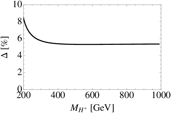
Now we evaluate the EDMs numerically. At first, in Fig. 5, we show the numerical improvement by the pinch contributions. Here we consider the electron EDM in the type-II 2HDM. The vertical axis in the Fig. 5 is difference of the gauge invariant EDM contribution and non-invariant one, $\Delta$ , defined as

\displaystyle\Delta=

\displaystyle\frac{(d_{e})_{\text{gauge non-inv.}}-(d_{e})_{\text{gauge inv.}}}{(d_{e})_{\text{gauge inv.}}},

(5.1)

where the gauge non-invariant EDM contribution $(d_{e})_{\text{gauge non-inv.}}$ is gotten by calculating only Barr-Zee diagrams [11, 12]. The horizontal axis is the mass of charged Higgs boson. We take $\tan\beta=10$ , $\lambda_{1}=\lambda_{3}=\lambda_{4}=\lambda_{5}\sin 2\phi=0.5$ and require the mass of lightest neutral scalar to be 126 GeV, then $\lambda_{2}$ is uniquely determined. We find that the pinch contributions are $5$ – $8$ %. This is not big improvement from the numerical point of view. However, we would like to emphasize that our result is now gauge invariant, which must be satisfied when we discuss observables.

Next, we discuss dependence of the electron EDM on the types of 2HDMs. The contributions from each types of diagrams to the electron EDM for type-I and II cases in Figs. 7 and 7, respectively. Here we take $\tan\beta=3$ or $50$ , and $\lambda_{1}=\lambda_{3}=\lambda_{4}=\lambda_{5}\sin 2\phi=0.5$ as a benchmark. We also require the mass of lightest neutral Higgs to be 126 GeV.

It is found that in the type-I case the $W$ boson contribution to $h\to\gamma\gamma$ is dominant and that all contributions to the electron EDM are proportional to $1/\tan^{2}\beta$ for $\tan\beta\gtrsim 1$ . On the other hand, the electron EDM in the type-II case is qualitatively different from the type-I case. Even when $\tan\beta$ is large, the $W$ boson and top quark contributions are not suppressed and the bottom quark and tau lepton contributions also become dominant due to the non-decoupling effect. Since the signs of the bottom quark and tau lepton contributions are opposite to that of the $W$ boson, the accidental cancellation occurs in some parameter region. Thus, the $\tan\beta$ dependence is non-trivial in the type-II case.

In Figs. 8, the electron EDM is shown in four types of 2HDMs as functions of $\tan\beta$ and charged Higgs boson mass. We take $\lambda_{1}=\lambda_{3}=\lambda_{4}=\lambda_{5}\sin 2\phi=0.5$ and $\lambda_{2}=0.25$ . The regions filled with red color in the figures show the excluded regions by the latest upper bound on electron EDM, which is derived by the ACME experiment,

\displaystyle|d_{e}|<

\displaystyle 8.7\times 10^{-29}e\text{ cm }(90\%~\text{CL \cite[cite]{[\@@bibref{}{Baron:2013eja}{}{}]}}).

(5.2)

The blue dashed lines are the future prospects given in Table 2.

experiments	sensitivities on $d_{e}$
Fr [16]	$1\times 10^{-29}e$ cm
YbF molecule [17]	$1\times 10^{-30}e$ cm
WN ion [18]	$1\times 10^{-30}e$ cm

Table 2: Future prospects on electron EDM.

The electron EDM in the type-X and Y models has similar behavior to the type-II and I ones, respectively, because leptons couple to $H_{2}$ in type-I and Y models, and to $H_{1}$ in type-II and X models. We find that type-II and type-X 2HDMs are strongly constrained by the recent ACME experimental result, except for regions where the cancellation among diagrams occurs, as shown in Fig. 8. Furthermore, the future experiments could cover wide parameter regions with charged Higgs mass smaller than 1 TeV even in type-I and Y cases.

Next let us consider the neutron EDM. Even when the Peccei-Quinn mechanism [19] is operative, the neutron EDM is generated by higher-dimensional CP-violating operators in QCD, such as quark EDMs and also cEDMs with mass dimension up to 5. The neutron EDM is evaluated from the up and down quarks EDM and cEDM with the QCD sum rules [20, 21, 22]. The evaluation still ${\cal O}(1)$ uncertainties from the excited state contribution to the correlation function [20], and also from input parameters [21]. In this paper we use the result in Ref. [22] since it gives more conservative prediction for the neutron EDM,

\displaystyle d_{n}=

\displaystyle 0.79d_{d}-0.20d_{u}+e(0.59d_{d}^{c}+0.30d_{u}^{c}).

(5.3)

Here, the Peccei-Quinn mechanism is assumed.

Before going to evaluate the neutron EDM, we discuss behaviors of the quark EDMs and cEDMs in the 2HDMs. We plot the contributions from each types of diagrams to the down and up quark EDMs and cEDMs in the type-I case in Figs. 10 and 10. The input parameters are the same as in Fig 7. We see that the $W$ boson and top quark contributions give the dominant contributions to the EDMs and cEDMs, respectively, and the $\tan\beta$ dependence is $1/\tan^{2}\beta$ , as expected from Eq. (4.18). It is found that the sizes of cEDMs and EDMs are comparable to each others so that both contributions have to be included in evaluation of the neutron EDM.

In Figs. 12 and 12, the contributions from each types of diagrams to the down and up quark EDMs and cEDMs in the type-II case are also shown. The EDMs and cEDMs have qualitatively different behaviors from the type-I case. We find that the largest contribution to the neutron EDM comes from down quark cEDM. The top quark loop dominates in the down quark cEDM (and also the up quark cEDM) for small $\tan\beta$ , while the bottom quark one quickly dominates it when $\tan\beta$ is large. The later comes from the non-decoupling effect. Thus, the neutron EDM would be enhanced when $\tan\beta$ is large. It is also found that the down quark EDM has similar behavior to the electron EDM in the type-II case, though it is smaller than the down quark cEDM in the neutron EDM.

Here, we ignore the QCD corrections to the quark EDMs and cEDMs. The QCD corrections may change them up to ${\cal O}(10)$ % [23, 24], while the neutron EDM evaluation from the quark EDMs and cEDMs may have larger uncertainties. See Ref. [24] for evaluation for the QCD corrections to the Barr-Zee diagrams.

Now we show the neutron EDM in four types of 2HDMs in Fig. 13. The regions filled with red color in Fig. 13 show the excluded region by the current neutron EDM data,

\displaystyle|d_{n}|<

\displaystyle 2.9\times 10^{-26}e\text{ cm }(90\%~\text{CL \cite[cite]{[\@@bibref{}{Baker:2006ts}{}{}]}}).

(5.4)

The blue dashed lines are the future prospects given in Table 3.

Table 3: Future prospects for neutron EDM

experiments	sensitivities on $\|d_{n}\|$
cyro EDM [25]	$1.7\times 10^{-28}e$ cm
PSI (Phase II) [26]	$5\times 10^{-28}e$ cm

It is found that the neutron EDM in the type-X case has similar behavior to the type-I in low $\tan\beta$ region because the down quark Yukawa couplings in these two types are the same. The difference in high $\tan\beta$ region between Figs. 13 and 13 is due to the large $\tan\beta$ enhancement of the tau lepton Yukawa coupling. The behavior of the neutron EDM in the type-Y case is quite similar to the type-II case. This is because the cEDM contribution is dominant in both cases.

It is found in comparison of Fig. 8 with Fig. 13 that both measurements of the electron and neutron EDMs are complementary to each others in order to discriminate the 2HDMs. We may choose one from the four models in future.

Before closing this section, we would like to give a comment on the constraints on the parameter space. We have shown that some parameter regions are constrained by EDMs in Figs. 8 and 13. The constrained regions have an overlap with other constraints, such as flavor physics [27, 28] or direct search of heavy Higgs bosons [29]. Note that it is known that the custodial $SU(2)$ symmetry is broken in the Higgs potential in 2HDMs with the CP violation, and $\rho$ parameter might deviate from one at the one loop level [30]. However, if heavy Higgs boson mass scale $M$ is large or if coupling $\lambda_{1}-\lambda_{5}$ are not large, this contribution is small. We checked that this contribution does not conflict with the current bound in all figure of this paper.

6 Conclusions and discussion

In this paper, we evaluated fermionic EDMs in 2HDMs with softly broken $Z_{2}$ symmetry. We started by calculating the Barr-Zee diagrams in a gauge invariant way by using the pinch technique. The modification by the gauge invariant calculation is $5$ – $8$ % numerically. This does not change the previous result drastically, but important because physical quantities must be calculated in a gauge invariant way. We evaluated the electron and neutron EDMs in all four types in the 2HDMs. We find that type-II and type-X 2HDMs are strongly constrained by the latest ACME experiment bound on the electron EDM. The electron and neutron EDM measurements will improve in the future experiments. They are possible to seek physics at ${\cal O}$ (10) TeV scale (Fig. 14). The electron and neutron EDMs have different sensitivities on the 2HDMs, and they are complementary to each other in discrimination of the type of 2HDMs.

We have not addressed that the contributions from non-Barr-Zee type diagrams in this paper. Although they are naively expected to be smaller than the contributions from the Barr-Zee diagrams, they would become important once experiments find the EDMs and start precise measurements. To evaluate them, we need to calculate all diagrams at two-loop level. This issue may be discussed elsewhere.

It is worth referring to relation between EWBG and EDMs. In the 2HDMs, it is known that EWBG may occur through a strongly first order electroweak phase transition [31, 32, 33, 34, 35, 36]. For example, Ref. [35] numerically showed that the 2HDMs with softly-broken $Z_{2}$ symmetry may accommodate a strongly first order phase transition when the lightest neutral Higgs boson is around 125 GeV. In order to achieve the EWBG, one needs some CP violation phases in Higgs potential. The EDM searches could indirectly constrain parameter space which achieve the EWBG. In this paper, we find that low $\tan\beta$ regions in 2HDMs are disfavored by electron EDM. On the other hand, in fact, a strongly first order phase transition, which is needed for EWBG, prefers low $\tan\beta$ region [35]. Therefore there is a tension between EWBG and current bound on the EDM.

Acknowledgments

The authors thank the Yukawa Institute for Theoretical Physics at Kyoto University, where this work was initiated during the YITP workshop on “LHC vs. Beyond the Standard Model (YITP-W-12-21)”, March 19-25, 2013, and also acknowledge the participants of the workshop for very active discussions. They would also like to thank Koji Tsumura, Eibun Senaha, Ryosuke Sato, Yasuhiro Yamamoto, and Motoi Endo for useful discussions and comments. The work of J.H. is supported by Grant-in-Aid for Scientific research from the Ministry of Education, Science, Sports, and Culture (MEXT), Japan, No. 24340047, No. 23104011 and No. 22244021, and also by World Premier International Research Center Initiative (WPI Initiative), MEXT, Japan. The figures for this paper were drawn using Feynmf [37].

Appendix A 2HDMs

In this appendix, we present mass spectrum and also interactions in 2HDMs, which are used in text.

A.1 Relations between mass and gauge eigenstates

While eight scalar fields are present in 2HDMs,

\displaystyle\sigma_{1,2},\ \pi_{1,2}^{\pm},\ \pi_{1,2}^{3},

as in Eq. (2.1), those states are not mass eigenstates, namely their mass matrices are not diagonalized. We call them the gauge eigenstates. Corresponding to them, there are eight mass eigenstates, which we denote them as

\displaystyle\begin{matrix}h_{1,2,3}&\text{(neutral Higgs bosons)},\\ H^{\pm}&\text{(charged Higgs bosons)},\\ \pi_{Z,W^{\pm}}&\text{(would-be NG bosons)}.\end{matrix}

These two-types of states are related with orthogonal or unitary matrices which diagonalize the mass matrices. For the fields which include would-be NG bosons the matrices are given as

	$\displaystyle\left(\begin{matrix}\pi_{Z}\\ \pi_{A}\\ \end{matrix}\right)=$	$\displaystyle\left(\begin{matrix}\cos\beta&\sin\beta\\ -\sin\beta&\cos\beta\end{matrix}\right)\left(\begin{matrix}\pi_{1}^{3}\\ \pi_{2}^{3}\end{matrix}\right),$
	$\displaystyle\left(\begin{matrix}\pi_{W^{\pm}}\\ H^{\pm}\\ \end{matrix}\right)=$	$\displaystyle\left(\begin{matrix}\cos\beta&\sin\beta\\ -\sin\beta&\cos\beta\end{matrix}\right)\left(\begin{matrix}\pi_{1}^{\pm}\\ \pi_{2}^{\pm}\end{matrix}\right).$		(A.1)

The matrix $U$ for physical neutral Higgs bosons is given by a 3 by 3 matrix as

\displaystyle\left(\begin{matrix}h_{1}\\ h_{2}\\ h_{3}\\ \end{matrix}\right)=

\displaystyle U^{T}\left(\begin{matrix}\sigma_{1}\\ \sigma_{2}\\ \pi_{A}\\ \end{matrix}\right)=\left(\begin{matrix}\omega_{h1}^{\sigma_{1}}&\omega_{h1}^{\sigma_{2}}&\omega_{h1}^{\pi_{A}}\\ \omega_{h2}^{\sigma_{1}}&\omega_{h2}^{\sigma_{2}}&\omega_{h2}^{\pi_{A}}\\ \omega_{h3}^{\sigma_{1}}&\omega_{h3}^{\sigma_{2}}&\omega_{h3}^{\pi_{A}}\end{matrix}\right)\left(\begin{matrix}\sigma_{1}\\ \sigma_{2}\\ \pi_{A}\end{matrix}\right)

(A.2)

where

\displaystyle\sum_{X}\omega_{i}^{X}\omega_{j}^{X}=\delta_{ij},\,\quad\sum_{i}\omega_{i}^{X}\omega_{i}^{Y}=\delta^{XY}.

(A.3)

These relations are useful to find relations among some couplings.

A.2 Higgs masses in 2HDMs

The mass terms for the neutral physical Higgs bosons are given by

\displaystyle{\cal L}\supset-\frac{1}{2}\left(\begin{matrix}\sigma_{1}&\sigma_{2}&\pi_{A}\end{matrix}\right){\cal\widetilde{M}}^{2}_{\text{N}}\left(\begin{matrix}\sigma_{1}\\ \sigma_{2}\\ \pi_{A}\end{matrix}\right),

(A.4)

where

$\displaystyle\left({\cal\widetilde{M}}^{2}_{\text{N}}\right)_{11}=$	$\displaystyle v_{1}^{2}\lambda_{1}+M^{2}\sin^{2}\beta,$
$\displaystyle\left({\cal\widetilde{M}}^{2}_{\text{N}}\right)_{22}=$	$\displaystyle v_{2}^{2}\lambda_{2}+M^{2}\cos^{2}\beta,$
$\displaystyle\left({\cal\widetilde{M}}^{2}_{\text{N}}\right)_{33}=$	$\displaystyle M^{2}-v^{2}\lambda_{5}\cos(2\phi),$
$\displaystyle\left({\cal\widetilde{M}}^{2}_{\text{N}}\right)_{21}=\left({\cal\widetilde{M}}^{2}_{\text{N}}\right)_{12}=$	$\displaystyle\left(v^{2}\lambda_{345}-M^{2}\right)\sin\beta\cos\beta,$
$\displaystyle\left({\cal\widetilde{M}}^{2}_{\text{N}}\right)_{31}=\left({\cal\widetilde{M}}^{2}_{\text{N}}\right)_{13}=$	$\displaystyle\frac{1}{2}v^{2}\lambda_{5}\sin(2\phi)\sin\beta,$
$\displaystyle\left({\cal\widetilde{M}}^{2}_{\text{N}}\right)_{32}=\left({\cal\widetilde{M}}^{2}_{\text{N}}\right)_{23}=$	$\displaystyle\frac{1}{2}v^{2}\lambda_{5}\sin(2\phi)\cos\beta,$	(A.5)

where

\displaystyle\lambda_{345}=

\displaystyle\lambda_{3}+\lambda_{4}+\lambda_{5}\cos(2\phi),

(A.6)

and $M^{2}$ is defined in Eq. (2.4). This mass matrix satisfies

\displaystyle{\cal\widetilde{M}}^{2}_{\text{N}}=

\displaystyle U\left(\begin{matrix}m_{h_{1}}^{2}&&\\ &m_{h_{2}}^{2}&\\ &&m_{h_{3}}^{2}\end{matrix}\right)U^{T}.

(A.7)

In large $M$ limit, we find the following expressions for mass and mixing angles.

	$\displaystyle m_{h_{1}}^{2}=$	$\displaystyle\frac{v_{1}^{4}\lambda_{1}+v_{2}^{4}\lambda_{2}+2v_{1}^{2}v_{2}^{2}\lambda_{345}}{v^{2}}+{\cal O}(M^{-2}),$
	$\displaystyle m_{h_{2}}^{2}=$	$\displaystyle M^{2}\left(1+{\cal O}(M^{-2})\right),$
	$\displaystyle m_{h_{3}}^{2}=$	$\displaystyle M^{2}\left(1+{\cal O}(M^{-2})\right).$

$\displaystyle\left(\begin{matrix}\omega^{\sigma_{1}}_{h_{1}}\\ \omega^{\sigma_{2}}_{h_{1}}\\ \omega^{\pi_{A}}_{h_{1}}\end{matrix}\right)=$	$\displaystyle\left(\begin{matrix}\cos\beta\left(1-X\sin^{2}\beta\right)\\ \sin\beta\left(1+X\cos^{2}\beta\right)\\ -\frac{v_{1}v_{2}\lambda_{5}\sin(2\phi)}{M^{2}}\end{matrix}\right)+{\cal O}(M^{-4}),$
$\displaystyle\left(\begin{matrix}\omega^{\sigma_{1}}_{h_{2}}\\ \omega^{\sigma_{2}}_{h_{2}}\\ \omega^{\pi_{A}}_{h_{2}}\end{matrix}\right)=$	$\displaystyle\left(\begin{matrix}-\sin\beta\sin\theta\\ \cos\beta\sin\theta\\ \cos\theta\end{matrix}\right)+{\cal O}(M^{-2}),$
$\displaystyle\left(\begin{matrix}\omega^{\sigma_{1}}_{h_{3}}\\ \omega^{\sigma_{2}}_{h_{3}}\\ \omega^{\pi_{A}}_{h_{3}}\end{matrix}\right)=$	$\displaystyle\left(\begin{matrix}-\sin\beta\cos\theta\\ \cos\beta\cos\theta\\ -\sin\theta\end{matrix}\right)+{\cal O}(M^{-2}),$	(A.8)

where

	$\displaystyle\tan(2\theta)=$	$\displaystyle\frac{-(\cos^{2}\beta-\sin^{2}\beta)}{\sin^{2}\beta\cos^{2}\beta\left(\lambda_{1}+\lambda_{2}-2\lambda_{345}\right)+\lambda_{5}\cos 2\phi}\lambda_{5}\sin(2\phi),$
	$\displaystyle X=$	$\displaystyle\frac{v_{1}^{2}\lambda_{1}-v_{2}^{2}\lambda_{2}-(v_{1}^{2}-v_{2}^{2})\lambda_{345}}{M^{2}}.$		(A.9)

A.3 Interactions in 2HDMs

Couplings which are relevant to calculation for the gauge invariant Barr-Zee contributions are written in this subsection. Our convention of the sign in covariant derivative is

\displaystyle D_{\mu}=

\displaystyle\partial_{\mu}+igV_{\mu}.

(A.10)

A.3.1 $V$ - $\bar{f}$ - $f$ couplings

These couplings are the same as the SM case, but we show them here to establish our conventions. For neutral gauge bosons,

\displaystyle{\cal L}\supset

\displaystyle-\sum_{G=\gamma,Z}\overline{f}\gamma^{\mu}g_{Gff}fG_{\mu},

(A.11)

where $g_{Gff}$ contains chirality structure,

\displaystyle g_{Gff}=g_{Gff}^{L}P_{L}+g_{Gff}^{R}P_{R},

(A.12)

where

$\displaystyle g_{\gamma ff}^{L}=$	$\displaystyle eQ,$
$\displaystyle g_{\gamma ff}^{R}=$	$\displaystyle eQ,$
$\displaystyle g_{Zff}^{L}=$	$\displaystyle\frac{e}{sc}\left(T^{3}-s^{2}Q\right),$
$\displaystyle g_{Zff}^{R}=$	$\displaystyle\frac{e}{sc}\left(-s^{2}Q\right).$	(A.13)

For $W$ boson,

\displaystyle{\cal L}\supset

\displaystyle-\frac{1}{\sqrt{2}}\overline{u}\gamma^{\mu}g_{Wud}dW^{+}_{\mu}+h.c.,

(A.14)

where

\displaystyle g_{Wud}=

\displaystyle V_{\text{CKM}}\frac{e}{s}P_{L},

(A.15)

where $V_{\text{CKM}}$ is for the CKM matrix.

A.3.2 Yukawa couplings

The Yukawa interaction terms are described as

\displaystyle-\left(\begin{matrix}\overline{u}&\overline{d}\end{matrix}\right)\left(\begin{matrix}m_{u}^{\text{diag.}}+\sum_{s}g_{uus}s&\sum_{s}g_{\overline{u}ds^{+}}s^{+}\\ \sum_{s}g_{\overline{d}us^{-}}s^{-}&m_{d}^{\text{diag.}}+\sum_{s}g_{dds}s\end{matrix}\right)\left(\begin{matrix}u\\ d\end{matrix}\right),

(A.16)

where $s={h_{1},h_{2},h_{3},\pi_{Z}}$ , and $s^{\pm}={H^{\pm},\pi_{W^{\pm}}}$ . We define $g^{V}$ and $g^{A}$ as

\displaystyle g=

\displaystyle g^{V}+i\gamma^{5}g^{A}.

(A.17)

Finally we find explicit expressions of the couplings. For the neutral Higgs bosons,

$\displaystyle g_{uuh}^{V}=$	$\displaystyle\frac{m_{u}^{\text{diag.}}}{v}\frac{1}{\sin\beta}\omega_{h}^{\sigma_{2}},$
$\displaystyle g_{uuh}^{A}=$	$\displaystyle\frac{m_{u}^{\text{diag.}}}{v}\frac{1}{\tan\beta}\omega_{h}^{\pi_{A}},$
$\displaystyle g_{ddh}^{V}=$	$\displaystyle\begin{cases}\frac{m_{d}^{\text{diag.}}}{v}\frac{1}{\cos\beta}\omega_{h}^{\sigma_{1}}&(i=1)\\ \frac{m_{d}^{\text{diag.}}}{v}\frac{1}{\sin\beta}\omega_{h}^{\sigma_{2}}&(i=2)\end{cases},$
$\displaystyle g_{ddh}^{A}=$	$\displaystyle\begin{cases}\frac{m_{d}^{\text{diag.}}}{v}\tan\beta\omega_{h}^{\pi_{A}}&(i=1)\\ -\frac{m_{d}^{\text{diag.}}}{v}\frac{1}{\tan\beta}\omega_{h}^{\pi_{A}}&(i=2)\end{cases}.$	(A.18)

Here, $i$ corresponds to the same suffix of $H_{i}$ which couples to down-type quarks.

For the physical charged Higgs boson,

$\displaystyle g_{\overline{u}dH^{+}}^{V}$	$\displaystyle=\frac{1}{\sqrt{2}}\left(V_{\text{CKM}}\frac{m_{d}^{\text{diag.}}}{v_{i}}\left(-\delta_{1i}\sin\beta+\delta_{2i}\cos\beta\right)-\frac{m_{u}^{\text{diag.}}}{v_{2}}V_{\text{CKM}}\cos\beta\right),$
$\displaystyle g_{\overline{u}dH^{+}}^{A}$	$\displaystyle=-\frac{i}{\sqrt{2}}\left(V_{\text{CKM}}\frac{m_{d}^{\text{diag.}}}{v_{i}}\left(-\delta_{1i}\sin\beta+\delta_{2i}\cos\beta\right)+\frac{m_{u}^{\text{diag.}}}{v_{2}}V_{\text{CKM}}\cos\beta\right),$
$\displaystyle g_{\overline{d}uH^{-}}^{V}$	$\displaystyle=-\frac{1}{\sqrt{2}}\left(V_{\text{CKM}}^{\dagger}\frac{m_{u}^{\text{diag.}}}{v_{2}}\cos\beta-\frac{m_{d}^{\text{diag.}}}{v_{i}}V_{\text{CKM}}^{\dagger}\left(-\delta_{1i}\sin\beta+\delta_{2i}\cos\beta\right)\right),$
$\displaystyle g_{\overline{d}uH^{-}}^{A}$	$\displaystyle=\frac{i}{\sqrt{2}}\left(V_{\text{CKM}}^{\dagger}\frac{m_{u}^{\text{diag.}}}{v_{2}}\cos\beta+\frac{m_{d}^{\text{diag.}}}{v_{i}}V_{\text{CKM}}^{\dagger}\left(-\delta_{1i}\sin\beta+\delta_{2i}\cos\beta\right)\right),$	(A.19)

where $i$ in the suffix is again the same suffix of $H_{i}$ which couples to down-type quarks. Sometime the followings are useful:

$\displaystyle g_{\overline{u}dH^{+}}$	$\displaystyle=g_{\overline{u}dH^{+}}^{L}P_{L}+g_{\overline{u}dH^{+}}^{R}P_{R}$
	$\displaystyle=+\sqrt{2}\left[\left(-\frac{m_{u}^{\text{diag.}}}{v}V_{\text{CKM}}\frac{1}{\tan\beta}\right)P_{L}+\left(V_{\text{CKM}}\frac{m_{d}^{\text{diag.}}}{v}\left(-\delta_{1i}\tan\beta+\delta_{2i}\frac{1}{\tan\beta}\right)\right)P_{R}\right],$
$\displaystyle g_{\overline{d}uH^{-}}$	$\displaystyle=g_{\overline{d}uH^{-}}^{L}P_{L}+g_{\overline{d}uH^{-}}^{R}P_{R}$
	$\displaystyle=-\sqrt{2}\left[\left(-\frac{m_{d}^{\text{diag.}}}{v}V_{\text{CKM}}^{\dagger}\left(-\delta_{1i}\tan\beta+\delta_{2i}\frac{1}{\tan\beta}\right)\right)P_{L}+\left(V_{\text{CKM}}^{\dagger}\frac{m_{u}^{\text{diag.}}}{v}\frac{1}{\tan\beta}\right)P_{R}\right].$	(A.20)

A.3.3 ${\cal L}_{\mbox{\scriptsize WWW}}$

These couplings are the same as the SM case, but we show them here to establish our conventions.

$\displaystyle{\cal L}\supset$	$\displaystyle-\sum_{G=\gamma,Z}ig_{WWG}\biggl\{(\partial^{\alpha}W^{+\beta})W^{-\mu}G^{\nu}(g_{\alpha\mu}g_{\beta\nu}-g_{\alpha\nu}g_{\beta\mu})$
	$\displaystyle\hskip 85.35826pt+W^{+\beta}(\partial^{\alpha}W^{-\mu})G^{\nu}(g_{\alpha\nu}g_{\beta\mu}-g_{\alpha\beta}g_{\mu\nu})$
	$\displaystyle\hskip 85.35826pt+W^{+\beta}W^{-\mu}(\partial^{\alpha}G^{\nu})(g_{\alpha\beta}g_{\mu\nu}-g_{\alpha\mu}g_{\beta\nu})\biggr\},$	(A.21)

where

	$\displaystyle g_{WW\gamma}=$	$\displaystyle e,$
	$\displaystyle g_{WWZ}=$	$\displaystyle\frac{e}{s}c.$		(A.22)

A.3.4 $W$ - $W$ - $h$ couplings

\displaystyle{\cal L}\supset

\displaystyle\sum_{h}g_{WWh}W^{+}_{\mu}W^{-\mu}h+\frac{1}{2}g_{ZZh}Z_{\mu}Z^{\mu}h,

(A.23)

where

	$\displaystyle g_{WWh}=$	$\displaystyle 2\frac{m_{W}^{2}}{v}\left[\cos\beta\omega^{\sigma_{1}}_{h}+\sin\beta\omega^{\sigma_{2}}_{h}\right],$
	$\displaystyle g_{ZZh}=$	$\displaystyle 2\frac{m_{Z}^{2}}{v}\left[\cos\beta\omega^{\sigma_{1}}_{h}+\sin\beta\omega^{\sigma_{2}}_{h}\right].$		(A.24)

By using Eq. (A.3), we find that

\displaystyle\sum_{h}g_{\ell\ell h}^{A}g_{WWh}=0.

(A.25)

A.3.5 $V$ - $H^{+}$ - $H^{-}$ couplings

\displaystyle{\cal L}\supset

\displaystyle+i\left(H^{+}\partial_{\mu}H^{-}-H^{-}\partial_{\mu}H^{+}\right)\left(g_{\gamma H^{+}H^{-}}A^{\mu}+g_{ZH^{+}H^{-}}Z^{\mu}\right),

(A.26)

where

	$\displaystyle g_{\gamma H^{+}H^{-}}=$	$\displaystyle e,$
	$\displaystyle g_{ZH^{+}H^{-}}=$	$\displaystyle\frac{1}{2}\frac{e}{sc}(c^{2}-s^{2}).$		(A.27)

A.3.6 $W^{\pm}$ - $H^{\mp}$ - $h$ couplings

	$\displaystyle{\cal L}\supset$	$\displaystyle+ig_{W^{-}H^{+}h}\left(h\partial_{\mu}H^{+}-H^{+}\partial_{\mu}h\right)W^{-\mu}$
		$\displaystyle+ig_{W^{+}H^{-}h}\left(h\partial_{\mu}H^{-}-H^{-}\partial_{\mu}h\right)W^{+\mu},$		(A.28)

where

\displaystyle g_{W^{\pm}H^{\mp}h}=

\displaystyle\pm\frac{1}{2}\frac{e}{s}\left(-\sin\beta\omega^{\sigma_{1}}_{h}+\cos\beta\omega^{\sigma_{2}}_{h}\mp i\omega^{\pi_{A}}_{h}\right).

(A.29)

By using Eq. (A.3), we find that

\displaystyle\sum_{h}g_{W^{+}H^{-}h}g_{WWh}=0.

(A.30)

A.3.7 $s^{+}$ - $s^{-}$ - $h$ couplings

$\displaystyle{\cal L}\supset$	$\displaystyle+g_{H^{+}H^{-}h}H^{+}H^{-}h$
	$\displaystyle+g_{\pi_{W^{+}}\pi_{W^{-}}h}\pi_{W^{+}}\pi_{W^{-}}h$
	$\displaystyle+g_{\pi_{W^{+}}H^{-}h}\pi_{W^{+}}H^{-}h+g_{H^{+}\pi_{W^{-}}h}H^{+}\pi_{W^{-}}h$
	$\displaystyle+\frac{1}{2}g_{\pi_{Z}\pi_{Z}h}\pi_{Z}\pi_{Z}h,$	(A.31)

where

$\displaystyle g_{H^{+}H^{-}h}=$	$\displaystyle+\frac{v_{1}}{v^{2}}\left(-v_{1}^{2}\lambda_{3}+v_{2}^{2}(-\lambda_{1}+\lambda_{4}+\lambda_{5}\cos(2\phi))\right)\omega^{\sigma_{1}}_{h}$
	$\displaystyle+\frac{v_{2}}{v^{2}}\left(-v_{2}^{2}\lambda_{3}+v_{1}^{2}(-\lambda_{2}+\lambda_{4}+\lambda_{5}\cos(2\phi))\right)\omega^{\sigma_{2}}_{h}$
	$\displaystyle+\frac{v_{1}v_{2}}{v}\lambda_{5}\sin(2\phi)\omega^{\pi_{A}}_{h},$
$\displaystyle g_{\pi_{W^{+}}\pi_{W^{-}}h}=$	$\displaystyle-\frac{m_{h}^{2}}{2m_{W}^{2}}g_{WWh},$
$\displaystyle g_{\pi_{W^{+}}H^{-}h}=$	$\displaystyle-\frac{m_{H^{\pm}}^{2}-m_{h}^{2}}{m_{W}}g_{W^{+}H^{-}h},$
$\displaystyle g_{H^{+}\pi_{W^{-}}h}=$	$\displaystyle+\frac{m_{H^{\pm}}^{2}-m_{h}^{2}}{m_{W}}g_{W^{-}H^{+}h},$
$\displaystyle g_{\pi_{Z}\pi_{Z}h}=$	$\displaystyle-\frac{m_{h}^{2}}{2m_{Z}^{2}}g_{ZZh}.$	(A.32)

A.3.8 $W^{\pm}$ - $\pi^{\mp}$ - $h$ couplings

	$\displaystyle{\cal L}\supset$	$\displaystyle+ig_{W^{-}\pi^{+}h}\left(h\partial_{\mu}\pi^{+}-\pi^{+}\partial_{\mu}h\right)W^{-\mu}$
		$\displaystyle+ig_{W^{+}\pi^{-}h}\left(h\partial_{\mu}\pi^{-}-\pi^{-}\partial_{\mu}h\right)W^{+\mu},$		(A.33)

where

\displaystyle g_{W^{\pm}\pi^{\mp}h}=

\displaystyle\pm\frac{1}{2m_{W}}g_{WWh}.

(A.34)

A.3.9 $V$ - $W^{\pm}$ - $\pi^{\mp}$ couplings

\displaystyle{\cal L}\supset

\displaystyle+\sum_{G=\gamma,Z}\left(g_{GW^{-}\pi^{+}}G_{\mu}W^{-\mu}\pi^{+}+g_{GW^{+}\pi^{-}}G_{\mu}W^{+\mu}\pi^{-}\right),

(A.35)

where

	$\displaystyle g_{\gamma W^{\mp}\pi^{\pm}}$	$\displaystyle=+em_{W},$
	$\displaystyle g_{ZW^{\mp}\pi^{\pm}}$	$\displaystyle=-esm_{Z}.$		(A.36)

A.3.10 Some four-point couplings

$\displaystyle{\cal L}\supset$	$\displaystyle+g_{H^{-}\pi_{W^{+}}\pi_{W^{-}}\pi_{W^{+}}}H^{-}\pi_{W^{+}}\pi_{W^{-}}\pi_{W^{+}}$
	$\displaystyle+\frac{1}{2}g_{H^{-}\pi_{W^{+}}\pi_{Z}\pi_{Z}}H^{-}\pi_{W^{+}}\pi_{Z}\pi_{Z}$
	$\displaystyle+g_{H^{-}\pi_{W^{+}}H^{-}H^{+}}H^{-}\pi_{W^{+}}H^{-}H^{+},$	(A.37)

where

$\displaystyle g_{H^{-}\pi_{W^{+}}\pi_{W^{-}}\pi_{W^{+}}}=$	$\displaystyle\sum_{h}\frac{1}{m_{W}}g_{W^{+}H^{-}h}g_{\pi_{W^{+}}\pi_{W^{-}}h},$
$\displaystyle g_{H^{-}\pi_{W^{+}}\pi_{Z}\pi_{Z}}=$	$\displaystyle\sum_{h}\frac{1}{m_{W}}g_{W^{+}H^{-}h}g_{\pi_{Z}\pi_{Z}h},$
$\displaystyle g_{H^{-}\pi_{W^{+}}H^{-}H^{+}}=$	$\displaystyle\sum_{h}\frac{1}{m_{W}}g_{W^{+}H^{-}h}g_{H^{+}H^{-}h}.$	(A.38)

Appendix B EDM formula details

In this section we present formulae for the Barr-Zee contributions to fermionic EDMs and cEDMs.

B.1 Fermion loops ( $h\gamma\gamma$ and $hZ\gamma$ )

After substituting Eqs. (3.19) and (3.20) for Eq. (4.3), we find the fermion loop contributions to the EDMs for fermion $\ell$ are

	$\displaystyle\left(\frac{d_{\ell}}{e}\right)_{\text{fermion}}$	$\displaystyle=-\frac{m_{\ell}}{(4\pi)^{4}}\sqrt{2}G_{F}\sum_{f}\sum_{h}\sum_{G=\gamma,Z}N_{c}Q_{f}\left(g_{G\ell\ell}^{L}+g_{G\ell\ell}^{R}\right)$
		$\displaystyle\quad\quad\quad\times\Biggl[\frac{g_{\ell\ell h}^{A}}{m_{\ell}/v}\frac{g_{ffh}^{V}}{m_{f}/v}{\cal I}_{1}^{G}(m_{f},m_{h})+\frac{g_{\ell\ell h}^{V}}{m_{\ell}/v}\frac{g_{ffh}^{A}}{m_{f}/v}{\cal I}_{2}^{G}(m_{f},m_{h})\Biggr],$		(B.1)

where

	$\displaystyle{\cal I}^{G}_{1}(m_{f},m_{h})=$	$\displaystyle\left(g_{Gff}^{L}+g_{Gff}^{R}\right)\frac{m_{f}^{2}}{m_{h}^{2}-m_{G}^{2}}\left(I_{1}(m_{f},m_{G})-I_{1}(m_{f},m_{h})\right),$
	$\displaystyle{\cal I}^{G}_{2}(m_{f},m_{h})=$	$\displaystyle\left(g_{Gff}^{L}+g_{Gff}^{R}\right)\frac{m_{f}^{2}}{m_{h}^{2}-m_{G}^{2}}\left(I_{2}(m_{f},m_{G})-I_{2}(m_{f},m_{h})\right),$		(B.2)

and where^#4^#4 #4 The functions $f(z)$ and $g(z)$ in Refs. [10, 11] are related to $I_{1}$ and $I_{2}$ as follows: $\displaystyle I_{1}(m_{1},m_{2})=-2\frac{m_{2}^{2}}{m_{1}^{2}}f\left(\frac{m_{1}^{2}}{m_{2}^{2}}\right),\quad I_{2}(m_{1},m_{2})=-2\frac{m_{2}^{2}}{m_{1}^{2}}g\left(\frac{m_{1}^{2}}{m_{2}^{2}}\right).$ (B.3)

	$\displaystyle I_{1}(m_{1},m_{2})=$	$\displaystyle\int_{0}^{1}dz\left(1-2z(1-z)\right)\frac{m_{2}^{2}}{m_{1}^{2}-m_{2}^{2}z(1-z)}\ln\frac{m_{2}^{2}z(1-z)}{m_{1}^{2}},$
	$\displaystyle I_{2}(m_{1},m_{2})=$	$\displaystyle\int_{0}^{1}dz\frac{m_{2}^{2}}{m_{1}^{2}-m_{2}^{2}z(1-z)}\ln\frac{m_{2}^{2}z(1-z)}{m_{1}^{2}}.$		(B.4)

B.2 Charged Higgs loops ( $h\gamma\gamma$ and $hZ\gamma$ )

By substituting the result in Eq. (3.21) into Eq. (4.3), we find the charged Higgs contribution to the EDMs,

\displaystyle\left(\frac{d_{\ell}}{e}\right)_{\text{scalar}}=+\frac{m_{\ell}}{(4\pi)^{4}}\sqrt{2}G_{F}\sum_{h}\sum_{G=\gamma,Z}

\displaystyle\left(g_{G\ell\ell}^{L}+g_{G\ell\ell}^{R}\right)\frac{g_{\ell\ell h}^{A}}{m_{\ell}/v}\frac{g_{H^{+}H^{-}h}}{v}{\cal I}^{G}_{3}(m_{H^{\pm}},m_{h}),

(B.5)

where

	$\displaystyle{\cal I}^{G}_{3}(m_{H^{\pm}},m_{h})=$	$\displaystyle-\frac{1}{2}g_{GH^{+}H^{-}}\frac{v^{2}}{m_{h}^{2}-m_{G}^{2}}$
		$\displaystyle\quad\quad\times\Biggl[\left(I_{1}(m_{H^{\pm}},m_{G})-I_{1}(m_{H^{\pm}},m_{h})\right)-\left(I_{2}(m_{H^{\pm}},m_{G})-I_{2}(m_{H^{\pm}},m_{h})\right)\Biggr].$		(B.6)

B.3 $W$ loops ( $h\gamma\gamma$ and $hZ\gamma$ )

The EDM contributions from $W$ boson loops are

\displaystyle\left(\frac{d_{\ell}}{e}\right)_{W}=

\displaystyle+\frac{m_{\ell}}{(4\pi)^{4}}\sqrt{2}G_{F}\sum_{h}\sum_{G=\gamma,Z}\left(g_{G\ell\ell}^{L}+g_{G\ell\ell}^{R}\right)\frac{g_{\ell\ell h}^{A}}{m_{\ell}/v}\frac{g_{WWh}}{2m_{W}^{2}/v}{\cal I}^{G}_{W}(m_{h}),

(B.7)

where

$\displaystyle{\cal I}^{G}_{W}(m_{h})$	$\displaystyle=g_{WWG}\frac{2m_{W}^{2}}{m_{h}^{2}-m_{G}^{2}}$
	$\displaystyle\times\Biggl[-\frac{1}{4}\left\{\left(6-\frac{m_{G}^{2}}{m_{W}^{2}}\right)+\left(1-\frac{m_{G}^{2}}{2m_{W}^{2}}\right)\frac{m_{h}^{2}}{m_{W}^{2}}\right\}\bigl[I_{1}(m_{W},m_{h})-I_{1}(m_{W},m_{G})\bigr]$
	$\displaystyle+\left\{\left(-4+\frac{m_{G}^{2}}{m_{W}^{2}}\right)+\frac{1}{4}\left(6-\frac{m_{G}^{2}}{m_{W}^{2}}+\left(1-\frac{m_{G}^{2}}{2m_{W}^{2}}\right)\frac{m_{h}^{2}}{m_{W}^{2}}\right)\right\}\bigl[I_{2}(m_{W},m_{h})-I_{2}(m_{W},m_{G})\bigr]\Biggr].$	(B.8)

We note that when one chooses $G=\gamma$ in Eq. (B.7) and drops $m_{h}^{2}/m_{W}^{2}$ terms in Eq. (B.8), the EDM contribution from $W$ boson loops becomes consistent with original result of Barr and Zee [10], where they ignored diagrams which contain only NG boson in the loop in Fig. 1 for simplicity and Higgs-NG bosons interaction is proportional to $m_{h}^{2}/m_{W}^{2}$ (see Eq. (A.32)).

B.4 $H^{\mp}W^{\pm}\gamma$

In this paper we compute for the first time the EDM contributions from $H^{\mp}W^{\pm}\gamma$ vertices which are generated by $W$ and charged Higgs boson loops. The detail of this derivation is given in Appendix C. The contributions to the EDMs are

\displaystyle\frac{d_{\ell}}{e}=

\displaystyle-\frac{m_{\ell}}{(4\pi)^{4}}\sqrt{2}G_{F}{\cal S}_{\ell}\sum_{h}\left(\frac{g_{\ell\ell h}^{A}}{m_{\ell}/v}\frac{g_{WWh}}{2m_{W}^{2}/v}\frac{e^{2}}{2s^{2}}{\cal I}_{4}(m_{h},m_{H^{\pm}})+\frac{g_{\ell\ell h}^{A}}{m_{\ell}/v}\frac{g_{H^{+}H^{-}h}}{v}{\cal I}_{5}(m_{h},m_{H^{\pm}})\right),

(B.9)

where

	$\displaystyle{\cal I}_{4}(m_{h},m_{H^{\pm}})=$	$\displaystyle\frac{m_{W}^{2}}{m_{H^{\pm}}^{2}-m_{W}^{2}}\left(I_{4}(m_{W},m_{h})-I_{4}(m_{H^{\pm}},m_{h})\right),$
	$\displaystyle{\cal I}_{5}(m_{h},m_{H^{\pm}})=$	$\displaystyle\frac{m_{W}^{2}}{m_{H^{\pm}}^{2}-m_{W}^{2}}\left(I_{5}(m_{W},m_{h})-I_{5}(m_{H^{\pm}},m_{h})\right),$		(B.10)

and where

$\displaystyle I_{4}(m_{1},m_{h})=$	$\displaystyle\int_{0}^{1}dz\left(z(1-z)^{2}-4(1-z)^{2}+\frac{m_{H^{\pm}}^{2}-m_{h}^{2}}{m_{W}^{2}}z(1-z)^{2}\right)$
	$\displaystyle\qquad\qquad\times\frac{m_{1}^{2}}{m_{W}^{2}(1-z)+m_{h}^{2}z-m_{1}^{2}z(1-z)}\ln\left(\frac{m_{W}^{2}(1-z)+m_{h}^{2}z}{m_{1}^{2}z(1-z)}\right),$
$\displaystyle I_{5}(m_{1},m_{h})=$	$\displaystyle 2\int_{0}^{1}dz\frac{m_{1}^{2}z(1-z)^{2}}{m_{H^{\pm}}^{2}(1-z)+m_{h}^{2}z-m_{1}^{2}z(1-z)}\ln\left(\frac{m_{H^{\pm}}^{2}(1-z)+m_{h}^{2}z}{m_{1}^{2}z(1-z)}\right).$	(B.11)

Here we have used the following relations among the coupling,

$\displaystyle\text{Im}\left(\frac{g_{\bar{\nu}eH^{+}}^{R}}{\sqrt{2}m_{e}/v}\frac{g_{W^{+}H^{-}h}}{e/(2s)}\right)=$	$\displaystyle\frac{g_{eeh}^{A}}{m_{e}/v},$
$\displaystyle\text{Im}\left(\frac{g_{\bar{u}dH^{+}}^{R}}{\sqrt{2}m_{d}/v}\frac{g_{W^{+}H^{-}h}}{e/(2s)}\right)=$	$\displaystyle\frac{g_{ddh}^{A}}{m_{d}/v},$
$\displaystyle\text{Im}\left(\frac{g_{\bar{d}uH^{-}}^{R}}{\sqrt{2}m_{u}/v}\frac{g_{W^{-}H^{+}h}}{e/(2s)}\right)=$	$\displaystyle\frac{g_{uuh}^{A}}{m_{u}/v}.$	(B.12)

B.5 CEDMs

The effective Hamiltonian for the cEDM is defined as Eq. (4.7). We find

\displaystyle d_{q}^{c}

\displaystyle=+\frac{m_{q}}{(4\pi)^{4}}\sqrt{2}G_{F}\sum_{f}\sum_{h}2g_{s}^{2}\frac{m_{f}^{2}}{m_{h}^{2}}\Biggl[\frac{g_{qqh}^{A}}{m_{q}/v}\frac{g_{ffh}^{V}}{m_{f}/v}I_{1}(m_{f},m_{h})+\frac{g_{qqh}^{V}}{m_{q}/v}\frac{g_{ffh}^{A}}{m_{f}/v}I_{2}(m_{f},m_{h})\Biggr].

(B.13)

Appendix C Derivation for effective $H^{-}W^{+}\gamma$ vertex

In this appendix, we present explicit derivation of the effective $H^{-}W^{+}\gamma$ vertex, which is generated from bosonic loop diagrams, in 2HDMs.

There are two types of loop diagrams; vertex corrections (Fig. 15) and wave function corrections (Fig. 16). The diagrams in Fig. 16 give nothing because of $C$ -invariance. The contributions from Fig. 16 is always proportional to $p_{2}^{\nu}$ . Thus they do not contribute to the on-shell amplitude of $H^{\mp}\to W^{\mp}\gamma$ nor the EDM at two-loop level by the same discussion in Sec. 3. Hence what we need to calculate are only the diagrams in Figs. 15, 16, and 16. In this section, we calculate these diagrams in ’t Hooft-Feynman gauge.

First, let us consider the diagrams in Figs. 15–15. These diagrams depend on the gauge fixing parameter of $W$ boson. We find

	$\displaystyle\sum\text{{\small Figs.~\ref{fig:a1}-\ref{fig:a6}}}$	$\displaystyle=+\frac{i}{(4\pi)^{D/2}}\Gamma(3-D/2)\left(p_{2\mu}p_{1\nu}-p_{2}p_{1}g_{\mu\nu}\right)\sum_{h}eg_{W^{+}H^{-}h}g_{WWh}$
		$\displaystyle\quad\times\int_{x+y+z=1}\frac{-2yz-4z+4-\frac{m_{H^{\pm}}^{2}-m_{h}^{2}}{m_{W}^{2}}2yz}{\left[m_{W}^{2}(1-z)+m_{h}^{2}z-p_{2}^{2}z(1-z)-2p_{1}p_{2}yz\right]^{3-D/2}}$
		$\displaystyle+\frac{i}{(4\pi)^{D/2}}g_{\mu\nu}\sum_{h}eg_{W^{+}H^{-}h}g_{WWh}$
		$\displaystyle\quad\times\Biggl[\Gamma(2-D/2)\int_{0}^{1}dz\frac{-(1+z)}{\left[m_{W}^{2}z+m_{h}^{2}(1-z)-p_{H}^{2}z(1-z)\right]^{2-D/2}}$
		$\displaystyle\quad-\frac{m_{H^{\pm}}^{2}-m_{h}^{2}}{m_{W}^{2}}\Gamma(2-D/2)\int_{0}^{1}dz\frac{\frac{1}{2}(-1+2z)}{\left[m_{W}^{2}z+m_{h}^{2}(1-z)-p_{H}^{2}z(1-z)\right]^{2-D/2}}$

		$\displaystyle\quad+\left(p_{H}^{2}-m_{H^{\pm}}^{2}\right)\Gamma(3-D/2)$
		$\displaystyle\quad\quad\quad\Biggl.\times\int_{x+y+z=1}\frac{1}{\left[m_{W}^{2}(1-z)+m_{h}^{2}z-p_{2}^{2}z(1-z)-2p_{1}p_{2}yz\right]^{3-D/2}}\Biggr],$		(C.1)

where $p_{H}^{2}=(p_{1}+p_{2})^{2}$ . We find $g_{\mu\nu}$ terms, which are not gauge invariant. We will show these terms are canceled with other diagrams, that is, the pinch contributions.

The diagrams in Figs. 15 and 15 are independent from the gauge fixing parameter.

$\displaystyle\text{Fig.~\ref{fig:b1} + Fig.~\ref{fig:b2}}=$	$\displaystyle-\frac{i}{(4\pi)^{D/2}}\Gamma(3-D/2)\left(p_{2\mu}p_{1\nu}-p_{2}p_{1}g_{\mu\nu}\right)\sum_{h}eg_{W^{+}H^{-}h}g_{H^{+}H^{-}h}$
	$\displaystyle\qquad\times\int_{x+y+z=1}\frac{4yz}{\left[m_{H^{\pm}}^{2}(1-z)+m_{h}^{2}z-p_{2}^{2}z(1-z)-2p_{1}p_{2}yz\right]^{3-D/2}}$
	$\displaystyle-\frac{i}{(4\pi)^{D/2}}\Gamma(2-D/2)g_{\mu\nu}\sum_{h}eg_{W^{+}H^{-}h}g_{H^{+}H^{-}h}$
	$\displaystyle\qquad\times\int_{0}^{1}dz\frac{-1+2z}{\left[m_{H^{\pm}}^{2}z+m_{h}^{2}(1-z)-p_{H}^{2}z(1-z)\right]^{2-D/2}}.$	(C.2)

Next we calculate the diagrams in Figs. 16 and 16. First we define the following notation for self-energies:

		$\displaystyle=i\Pi^{\mu}_{H^{-}W^{+}}(p)=ip^{\mu}\Pi_{H^{-}W^{+}}(p^{2}),$		(C.3)
		$\displaystyle=i\Pi_{H^{-}\pi_{W^{+}}}(p^{2}).$		(C.4)

The direction of the momentum of $\Pi_{H^{-}W^{+}}^{\mu}$ is shown in the figure. Using this notation, we find

	$\displaystyle\text{Fig.~\ref{fig:wavefunction_HW} + Fig.~\ref{fig:wavefunction_Hpi}}=$	$\displaystyle\frac{-ig_{\mu\nu}}{p_{H}^{2}-m_{W}^{2}}\left(-em_{W}i\Pi_{H^{-}\pi_{W^{+}}}(p_{H}^{2})-em_{W}^{2}\Pi_{H^{-}W^{+}}(p_{H}^{2})\right)$
		$\displaystyle+\left(p_{2}^{2}-m_{W}^{2}\right)\frac{-ig_{\mu\nu}}{p_{H}^{2}-m_{W}^{2}}\left(-e\Pi_{H^{-}W^{+}}(p_{H}^{2})\right).$		(C.5)

Here we ignored $p_{2}^{\mu}p_{2}^{\nu}$ terms because they do not contribute to the EDMs as we discussed in Sec. 3. Note that the $\left(p_{2}^{2}-m_{W}^{2}\right)$ term does not also contribute to the on-shell amplitudes nor the EDMs at two-loop level. If we calculate the EDMs with this term, we immediately see that $q^{2}$ dependence completely canceled out. Thus, we only need the first term in Eq. (C.5).

Fig. 17 shows the diagrams for $\Pi_{H^{-}W^{+}}(p^{2})$ . We find

	$\displaystyle i\Pi_{H^{-}W^{+}}(p^{2})=$	$\displaystyle+\frac{i}{(4\pi)^{D/2}}\Gamma(2-D/2)g_{WWh}g_{W^{+}H^{-}h}\int_{0}^{1}dx\frac{-(2-x)+\frac{m_{H^{\pm}}^{2}-m_{h}^{2}}{m_{W}^{2}}(x-\frac{1}{2})}{\left[m_{W}^{2}(1-x)+m_{h}^{2}x-p^{2}x(1-x)\right]^{2-D/2}}$
		$\displaystyle+\frac{i}{(4\pi)^{D/2}}\Gamma(2-D/2)g_{H^{+}H^{-}h}g_{W^{+}H^{-}h}\int_{0}^{1}dx\frac{1-2x}{\left[m_{H^{\pm}}^{2}x+m_{h}^{2}(1-x)-p^{2}x(1-x)\right]^{2-D/2}}.$		(C.6)

Fig. 18 shows the diagrams for $\Pi_{H^{-}\pi_{W^{+}}}(p^{2})$ . We find Figs. 18–18 are canceled by Fig. 18, so we do not calculate them. Fig. 18 is the counter term for $H$ – $\pi_{W}$ mixing, and it is also related with the counter terms for the Higgs tadpoles (Fig. 19),

\displaystyle\delta_{H^{-}\pi_{W^{+}}}=

\displaystyle\sum_{h}\frac{1}{m_{W}}g_{W^{+}H^{-}h}\delta_{h},

(C.7)

where $\delta$ ’s are defined through

\displaystyle{\cal L}\supset

\displaystyle-\delta_{H^{-}\pi_{W^{+}}}H^{-}\pi_{W^{+}}+\sum_{h}\delta_{h}h.

(C.8)

It is easy to find this relation by analyzing the Higgs potential. We take renormalization conditions in which all tadpole diagrams are completely canceled by their counter terms. Then $\delta_{H^{-}\pi_{W^{+}}}$ is not arbitrary but should be calculated from the tadpole diagrams and Eq. (C.8). We show the tadpole diagrams in Fig. 19.

After calculating tadpole diagrams, using Eq. (C.7), we find

$\displaystyle\text{Fig.~\ref{fig:ct_Hpi}}=$	$\displaystyle-\left(\text{Fig.~\ref{fig:g1}}+\text{Fig.~\ref{fig:g2}}+\text{Fig.~\ref{fig:g3}}+\text{Fig.~\ref{fig:g4}}\right)$
	$\displaystyle+i\sum_{h}\left(\frac{m_{H^{\pm}}^{2}-m_{h}^{2}}{2m_{W}^{3}}g_{WWh}g_{W^{+}H^{-}h}+\frac{g_{H^{+}H^{-}h}g_{W^{+}H^{-}h}}{m_{W}}\right)\int_{\ell}\frac{1}{\ell^{2}-m_{h}^{2}}$
	$\displaystyle-i\sum_{h}\frac{g_{H^{+}H^{-}h}g_{W^{+}H^{-}h}}{m_{W}}\int_{\ell}\frac{1}{\ell^{2}-m_{H^{\pm}}^{2}}$
	$\displaystyle+i\sum_{h}\frac{m_{h}^{2}}{2m_{W}^{3}}g_{H^{+}H^{-}h}g_{W^{+}H^{-}h}\int_{\ell}\frac{1}{\ell^{2}-m_{W}^{2}}.$	(C.9)

Now we have calculated all the diagrams shown in Fig. 18, and we find

$\displaystyle i\Pi_{H^{-}\pi_{W^{+}}}=$	$\displaystyle+\frac{\Gamma(2-D/2)}{(4\pi)^{D/2}}\frac{1}{2m_{W}}g_{WWh}g_{W^{+}H^{-}h}$
	$\displaystyle\quad\times\int_{0}^{1}dx\Biggl[\frac{p^{2}(1+2x)+m_{h}^{2}}{\left[m_{W}^{2}x+m_{h}^{2}(1-x)-p^{2}x(1-x)\right]^{2-D/2}}\Biggr.$
	$\displaystyle\qquad\qquad\Biggl.+\frac{m_{H^{\pm}}^{2}-m_{h}^{2}}{m_{W}^{2}}\frac{m_{W}^{2}-p^{2}(1-2x)}{\left[m_{W}^{2}x+m_{h}^{2}(1-x)-p^{2}x(1-x)\right]^{2-D/2}}\Biggr]$
	$\displaystyle-\frac{\Gamma(2-D/2)}{(4\pi)^{D/2}}\frac{1}{m_{W}}g_{H^{+}H^{-}h}g_{W^{+}H^{-}h}p^{2}\int_{0}^{1}dx\frac{1-2x}{\left[m_{H^{\pm}}^{2}x+m_{h}^{2}(1-x)-p^{2}x(1-x)\right]^{2-D/2}}.$	(C.10)

We have finished preparing to calculate Fig. 16 + Fig. 16. Substituting Eqs. (C.6) and (C.10) into the first term in Eq. (C.5), then we find

$\displaystyle\text{Fig.~\ref{fig:wavefunction_HW} + Fig.~\ref{fig:wavefunction_Hpi}}=$	$\displaystyle-ig_{\mu\nu}\frac{1}{(4\pi)^{D/2}}\Gamma(2-D/2)eg_{W^{+}H^{-}h}$
	$\displaystyle\times\Biggl[g_{WWh}\int_{0}^{1}dx\frac{-(1+x)+\frac{m_{H^{\pm}}^{2}-m_{h}^{2}}{2m_{W}^{2}}(1-2x)}{\left[m_{W}^{2}x+m_{h}^{2}(1-x)-p_{H}^{2}x(1-x)\right]^{2-D/2}}$
	$\displaystyle\quad+g_{WWh}\frac{p_{H}^{2}-m_{H^{\pm}}^{2}}{2(p_{H}^{2}-m_{W}^{2})}\int_{0}^{1}dx\frac{1}{\left[m_{W}^{2}x+m_{h}^{2}(1-x)-p_{H}^{2}x(1-x)\right]^{2-D/2}}$
	$\displaystyle\quad+g_{H^{+}H^{-}h}\int_{0}^{1}dx\frac{1-2x}{\left[m_{H^{\pm}}^{2}x+m_{h}^{2}(1-x)-p_{H}^{2}x(1-x)\right]^{2-D/2}}\Biggr].$	(C.11)

Here we dropped the $(p_{2}^{2}-m_{W}^{2})g_{\mu\nu}$ term because it does not contribute to what we are interested in. Note that the first term in the bracket in Eq. (C.11) is canceled with Eq. (C.1), and the second term is canceled with Eq. (C.2).

So far we have calculated many diagrams, vertex corrections and wave function corrections. The corrections are not so simple and some of them canceled out, so we give a short summary so far here. After summing up all the correction we have calculated so far, we find

		$\displaystyle+\frac{i}{(4\pi)^{D/2}}\Gamma(3-D/2)\left(p_{2\mu}p_{1\nu}-p_{2}p_{1}g_{\mu\nu}\right)$
		$\displaystyle\qquad\qquad\times\Biggl(+\sum_{h}eg_{W^{+}H^{-}h}g_{WWh}\int_{x+y+z=1}\frac{-2yz-4z+4-\frac{m_{H^{\pm}}^{2}-m_{h}^{2}}{m_{W}^{2}}2yz}{\left[m_{W}^{2}(1-z)+m_{h}^{2}z-p_{2}^{2}z(1-z)-2p_{1}p_{2}yz\right]^{3-D/2}}$
		$\displaystyle\qquad\qquad\qquad-\sum_{h}eg_{W^{+}H^{-}h}g_{H^{+}H^{-}h}\int_{x+y+z=1}\frac{4yz}{\left[m_{H^{\pm}}^{2}(1-z)+m_{h}^{2}z-p_{2}^{2}z(1-z)-2p_{1}p_{2}yz\right]^{3-D/2}}\Biggr)$
		$\displaystyle+\frac{i}{(4\pi)^{D/2}}g_{\mu\nu}\left(p_{H}^{2}-m_{H^{\pm}}^{2}\right)\sum_{h}eg_{W^{+}H^{-}h}g_{WWh}$
		$\displaystyle\qquad\qquad\times\Biggl[+\Gamma(3-D/2)\int_{x+y+z=1}\frac{1}{\left[m_{W}^{2}(1-z)+m_{h}^{2}z-p_{2}^{2}z(1-z)-2p_{1}p_{2}yz\right]^{3-D/2}}$
		$\displaystyle\qquad\qquad\qquad-\Gamma(2-D/2)\frac{1}{2(p_{H}^{2}-m_{W}^{2})}\int_{0}^{1}dx\frac{1}{\left[m_{W}^{2}x+m_{h}^{2}(1-x)-p_{H}^{2}x(1-x)\right]^{2-D/2}}\Biggr].$		(C.12)

Note that the last two terms are not gauge invariant in the sense that we discussed in Sec. 3. Since they are proportional to $p_{H}^{2}-m_{H^{\pm}}^{2}$ , if we take the charged Higgs boson on-shell, they are dropped and the result becomes gauge invariant. However, now we need to take the charged Higgs boson off-shell, so we still need some other terms to cancel them.

To find a gauge invariant set for the Barr-Zee diagrams, we need to take into account for the pinch contributions shown in Fig. 20. After pinching the fermion propagators with red color in Figs. 20 and 20, the pinch contributions for $H^{-}W^{+}\gamma$ effective vertex for the Barr-Zee diagrams arise. They are schematically shown in Figs. 20 and 20. We denote their contributions as $\Gamma^{\mu\nu}_{\text{P}}$ and $i\Pi_{\text{P}}$ , respectively. Then we find

	$\displaystyle i\Gamma_{\text{P}}^{\mu\nu}(p_{1},p_{2})=$	$\displaystyle-i\frac{\Gamma(3-D/2)}{(4\pi)^{D/2}}eg_{W^{+}H^{-}h}g_{WWh}g^{\mu\nu}$
		$\displaystyle\quad\times\left(p_{H}^{2}-m_{H^{\pm}}^{2}\right)\int_{x+y+z=1}\frac{1}{\left[m_{W}^{2}(1-z)+m_{h}^{2}z-p_{2}^{2}z(1-z)-2p_{1}p_{2}yz)\right]^{3-D/2}},$		(C.13)

	$\displaystyle i\Pi_{\text{P}}(p_{H}^{2})=$	$\displaystyle+\frac{\Gamma(2-D/2)}{(4\pi)^{2-D/2}}\frac{1}{2m_{W}}g_{W^{+}H^{-}h}g_{WWh}\left(p_{H}^{2}-m_{H^{\pm}}^{2}\right)$
		$\displaystyle\quad\times\int_{0}^{1}dx\frac{1}{\left[m_{W}^{2}x+m_{h}^{2}(1-x)-p_{H}^{2}x(1-x)\right]^{2-D/2}}.$		(C.14)

Using Eq. (C.5), we find that $\Gamma^{\mu\nu}_{\text{P}}$ and $i\Pi_{\text{P}}$ completely cancel the second term in Eq. (C.12), namely these pinch contributions really make the effective vertex correction gauge invariant.

References

[1] G. Aad et al. [ATLAS Collaboration], Phys. Lett. B 716, 1 (2012) [arXiv:1207.7214 [hep-ex]].
[2] S. Chatrchyan et al. [CMS Collaboration], Phys. Lett. B 716, 30 (2012) [arXiv:1207.7235 [hep-ex]].
[3] J. Baron et al. [ ACME Collaboration], arXiv:1310.7534 [physics.atom-ph].
[4] C. A. Baker, D. D. Doyle, P. Geltenbort, K. Green, M. G. D. van der Grinten, P. G. Harris, P. Iaydjiev and S. N. Ivanov et al., Phys. Rev. Lett. 97, 131801 (2006) [hep-ex/0602020].
[5] For reviews, M. Pospelov and A. Ritz, Annals Phys. 318, 119 (2005) [hep-ph/0504231];
M. Raidal, A. van der Schaaf, I. Bigi, M. L. Mangano, Y. K. Semertzidis, S. Abel, S. Albino and S. Antusch et al., Eur. Phys. J. C 57, 13 (2008) [arXiv:0801.1826 [hep-ph]];
T. Fukuyama, Int. J. Mod. Phys. A 27, 1230015 (2012) [arXiv:1201.4252 [hep-ph]].
[6] V. A. Kuzmin, V. A. Rubakov and M. E. Shaposhnikov, Phys. Lett. B 155, 36 (1985).
[7] A. G. Cohen, D. B. Kaplan and A. E. Nelson, Ann. Rev. Nucl. Part. Sci. 43, 27 (1993) [hep-ph/9302210].
[8] V. A. Rubakov and M. E. Shaposhnikov, Usp. Fiz. Nauk 166, 493 (1996) [Phys. Usp. 39, 461 (1996)] [hep-ph/9603208].
[9] M. Trodden, Rev. Mod. Phys. 71, 1463 (1999) [hep-ph/9803479].
[10] S. M. Barr and A. Zee, Phys. Rev. Lett. 65, 21 (1990) [Erratum-ibid. 65, 2920 (1990)].
[11] R. G. Leigh, S. Paban and R. M. Xu, Nucl. Phys. B 352, 45 (1991).
[12] D. Chang, W. -Y. Keung and T. C. Yuan, Phys. Rev. D 43, 14 (1991).
[13] G. Degrassi and A. Sirlin, Phys. Rev. D 46, 3104 (1992).
[14] G. Degrassi and A. Sirlin, Nucl. Phys. B 383, 73 (1992).
[15] A. Denner, Fortsch. Phys. 41, 307 (1993) [arXiv:0709.1075 [hep-ph]].
[16] Y. Sakemi, K. Harada, T. Hayamizu, M. Itoh, H. Kawamura, S. Liu, H. S. Nataraj and A. Oikawa et al., J. Phys. Conf. Ser. 302, 012051 (2011).
[17] D. M. Kara, I. J. Smallman, J. J. Hudson, B. E. Sauer, M. R. Tarbutt and E. A. Hinds, New J. Phys. 14, 103051 (2012) [arXiv:1208.4507 [physics.atom-ph]].
[18] D. Kawall, J. Phys. Conf. Ser. 295, 012031 (2011).
[19] R. D. Peccei and H. R. Quinn, Phys. Rev. Lett. 38, 1440 (1977).
[20] M. Pospelov and A. Ritz, Phys. Rev. D 63, 073015 (2001) [hep-ph/0010037].
[21] J. Hisano, J. Y. Lee, N. Nagata and Y. Shimizu, Phys. Rev. D 85, 114044 (2012) [arXiv:1204.2653 [hep-ph]].
[22] K. Fuyuto, J. Hisano, N. Nagata and K. Tsumura, arXiv:1308.6493 [hep-ph].
[23] G. Degrassi, E. Franco, S. Marchetti and L. Silvestrini, JHEP 0511, 044 (2005) [hep-ph/0510137].
[24] J. Hisano, K. Tsumura and M. J. S. Yang, Phys. Lett. B 713, 473 (2012) [arXiv:1205.2212 [hep-ph]].
[25] S. N. Balashov, K. Green, M. G. D. van der Grinten, P. G. Harris, H. Kraus, J. M. Pendlebury, D. B. Shiers and M. A. H. Tucker et al., arXiv:0709.2428 [hep-ex].
[26] K. Kirch, http://vmsstreamer1.fnal.gov/Lectures/Colloquium/presentations/130213Kirch.pdf
[27] U. Haisch, arXiv:0805.2141 [hep-ph].
[28] F. Mahmoudi and O. Stal, Phys. Rev. D 81, 035016 (2010) [arXiv:0907.1791 [hep-ph]].
[29] [CMS Collaboration], CMS-PAS-HIG-12-050.
[30] A. Pomarol and R. Vega, Nucl. Phys. B 413, 3 (1994) [hep-ph/9305272].
[31] N. Turok and J. Zadrozny, Nucl. Phys. B 358, 471 (1991).
[32] A. G. Cohen, D. B. Kaplan and A. E. Nelson, Phys. Lett. B 263, 86 (1991).
[33] J. M. Cline and P. -A. Lemieux, Phys. Rev. D 55, 3873 (1997) [hep-ph/9609240].
[34] L. Fromme, S. J. Huber and M. Seniuch, JHEP 0611, 038 (2006) [hep-ph/0605242].
[35] G. C. Dorsch, S. J. Huber and J. M. No, JHEP 1310, 029 (2013) [arXiv:1305.6610 [hep-ph]].
[36] J. M. Cline, K. Kainulainen and M. Trott, JHEP 1111, 089 (2011) [arXiv:1107.3559 [hep-ph]].
[37] T. Ohl, Comput. Phys. Commun. 90, 340 (1995) [hep-ph/9505351].

1 Introduction

2 Models

3 Effective vertices

3.1 Tensor structure of the effective vertices

3.2 Effective h​γ​γh\gamma\gamma and h​Z​γhZ\gamma vertices — WW boson loop —

3.3 Effective h​γ​γh\gamma\gamma and h​Z​γhZ\gamma vertices — fermion, H±H^{\pm} loop —

3.4 Effective H∓​W±​γH^{\mp}W^{\pm}\gamma vertices — WW, H±H^{\pm} loop —

4 EDM from Barr-Zee diagram

5 Numerical results

6 Conclusions and discussion

Acknowledgments

Appendix A 2HDMs

A.1 Relations between mass and gauge eigenstates

A.2 Higgs masses in 2HDMs

A.3 Interactions in 2HDMs

A.3.1 VV-f¯\bar{f}-ff couplings

A.3.2 Yukawa couplings

A.3.3 ℒWWW{\cal L}_{\mbox{\scriptsize WWW}}

A.3.4 WW-WW-hh couplings

A.3.5 VV-H+H^{+}-H−H^{-} couplings

A.3.6 W±W^{\pm}-H∓H^{\mp}-hh couplings

A.3.7 s+s^{+}-s−s^{-}-hh couplings

A.3.8 W±W^{\pm}-π∓\pi^{\mp}-hh couplings

A.3.9 VV-W±W^{\pm}-π∓\pi^{\mp} couplings

A.3.10 Some four-point couplings

Appendix B EDM formula details

B.1 Fermion loops (h​γ​γh\gamma\gamma and h​Z​γhZ\gamma)

B.2 Charged Higgs loops (h​γ​γh\gamma\gamma and h​Z​γhZ\gamma)

B.3 WW loops (h​γ​γh\gamma\gamma and h​Z​γhZ\gamma)

B.4 H∓​W±​γH^{\mp}W^{\pm}\gamma

B.5 CEDMs

Appendix C Derivation for effective H−​W+​γH^{-}W^{+}\gamma vertex

References

3.2 Effective $h\gamma\gamma$ and $hZ\gamma$ vertices — $W$ boson loop —

3.3 Effective $h\gamma\gamma$ and $hZ\gamma$ vertices — fermion, $H^{\pm}$ loop —

3.4 Effective $H^{\mp}W^{\pm}\gamma$ vertices — $W$ , $H^{\pm}$ loop —

A.3.1 $V$ - $\bar{f}$ - $f$ couplings

A.3.3 ${\cal L}_{\mbox{\scriptsize WWW}}$

A.3.4 $W$ - $W$ - $h$ couplings

A.3.5 $V$ - $H^{+}$ - $H^{-}$ couplings

A.3.6 $W^{\pm}$ - $H^{\mp}$ - $h$ couplings

A.3.7 $s^{+}$ - $s^{-}$ - $h$ couplings

A.3.8 $W^{\pm}$ - $\pi^{\mp}$ - $h$ couplings

A.3.9 $V$ - $W^{\pm}$ - $\pi^{\mp}$ couplings

B.1 Fermion loops ( $h\gamma\gamma$ and $hZ\gamma$ )

B.2 Charged Higgs loops ( $h\gamma\gamma$ and $hZ\gamma$ )

B.3 $W$ loops ( $h\gamma\gamma$ and $hZ\gamma$ )

B.4 $H^{\mp}W^{\pm}\gamma$

Appendix C Derivation for effective $H^{-}W^{+}\gamma$ vertex