跳到论文正文
W Papers独立论文阅读器 arXiv:1311.4696 论文正文 计算阅读时间 · 0%
引用这篇论文根据当前论文元数据生成,正式投稿前建议核对。


License: arXiv.org perpetual non-exclusive license
arXiv:1311.4696v1 [hep-th] 19 Nov 2013

KUNS-2467

A deformation of quantum affine algebra
in squashed WZNW models

Io Kawaguchi** * E-mail: io_\_at_\_gauge.scphys.kyoto-u.ac.jp and Kentaroh Yoshida†† † E-mail: kyoshida_\_at_\_gauge.scphys.kyoto-u.ac.jp

Department of Physics, Kyoto University
Kyoto 606-8502, Japan

Abstract

We proceed to study infinite-dimensional symmetries in two-dimensional squashed Wess-Zumino-Novikov-Witten (WZNW) models at the classical level. The target space is given by squashed S3 and the isometry is S​U​(2)L×U​(1)RSU(2)_{\rm L}\times U(1)_{\rm R} . It is known that S​U​(2)LSU(2)_{\rm L} is enhanced to a couple of Yangians. We reveal here that an infinite-dimensional extension of U​(1)RU(1)_{\rm R} is a deformation of quantum affine algebra, where a new deformation parameter is provided with the coefficient of the Wess-Zumino term. Then we consider the relation between the deformed quantum affine algebra and the pair of Yangians from the viewpoint of the left-right duality of monodromy matrices. The integrable structure is also discussed by computing the rr/ss-matrices that satisfy the extended classical Yang-Baxter equation. Finally two degenerate limits are discussed.

1 Introduction

The AdS/CFT correspondence [1, 2, 3] has been a fascinating topic in the study of string theory over the decade after Maldacena’s proposal. A tremendous amount of works have been devoted to test and generalize it. Nowadays, the research area covers diverse subjects. A great achievement in the recent progress is the discovery of the integrable structure behind the AdS/CFT correspondence (For a comprehensive review on this subject, see [4]).

In the string-theory side, the integrable structure of two-dimensional string sigma-models with target spacetime AdS5×{}_{5}\timesS5 plays an important role [5]. It is closely related to the fact that AdS5×{}_{5}\timesS5 is described as a symmetric coset. It leads to an infinite number of the conserved charges constructed, for example, by following the pioneering works [6, 7, 8, 9, 10] (For a comprehensive textbook see [11]). The symmetric cosets that potentially may lead to a holographic interpretation are classified, including spacetime fermions [12].

The next interesting issue is to consider integrable deformations of the AdS/CFT correspondence. There are two approaches. The one is an algebraic approach based on qq-deformations of the world-sheet S-matrix [13, 14, 15, 16, 17]. The deformed S-matrices are explicitly constructed, while the target-space geometry is unclear. The other is a geometric approach based on deformations of target spaces of the sigma models. It seems likely that the deformed geometries are represented by non-symmetric cosets [18] in comparison to AdS5×{}_{5}\timesS5 and hence the prescription for symmetric cosets is not available any more. It is necessary to develop a new method to argue the integrability.

In the latter approach, there is a long history (For classic papers see [19, 20, 21]). Motivated by integrable deformations of AdS/CFT, a series of works have been done on squashed S3 and warped AdS3 [22, 24, 25, 28, 26, 27, 29, 23, 30]. Some specific higher-dimensional cases are discussed in [31]. Remarkably, the classical integrable structure of deformed sigma models was recently shown for arbitrary compact Lie groups and the coset cousins by Delduc, Magro and Vicedo [32]. Then, they successively presented a qq-deformation of the AdS5×{}_{5}\timesS5 superstring [33].

Based on the latter approach, we are here concerned with the classical integrable structure of two-dimensional Wess-Zumino-Novikov-Witten (WZNW) models with the target space squashed S3 . The isometry is given by S​U​(2)L×U​(1)RSU(2)_{\rm L}\times U(1)_{\rm R} . It is partly explained in [24] that there exist a couple of Yangian algebras based on S​U​(2)LSU(2)_{\rm L} by explicit constructions of non-local conserved charges and direct computations of the Poisson brackets of the charges.

In this paper we consider an infinite-dimensional extension of U​(1)RU(1)_{\rm R} . In the case without the Wess-Zumino term, it is just a classical analogue of a quantum affine algebra [26]. When the Wess-Zumino term is added, an additional constant parameter is introduced as its coefficient. A natural question is what happens to the quantum affine algebra. As one may easily guess, a new kind of deformation is induced by the presence of the Wess-Zumino term. The resulting algebra is a classical analogue of the deformed quantum affine algebra. So far, it is not clear what is the mathematical formulation of the deformed quantum affine algebra, though it seems likely to be a two-parameter quantum toroidal algebra [34]. In order to answer the question, it is necessary to see the first realization of the two-parameter quantum toroidal algebra.

This paper is organized as follows. In section 2 the classical action of the squashed WZNW models is introduced. In section 3 we consider the classical integrable structure based on S​U​(2)LSU(2)_{\rm L} . This is called the left description. We present a couple of Lax pairs and the associated monodromy matrices. The classical rr/ss-matrices are shown to satisfy the extended classical Yang-Baxter equation. The infinite-dimensional extensions of S​U​(2)LSU(2)_{\rm L} are Yangians. In section 4 we argue the classical integrable structure based on U​(1)RU(1)_{\rm R} . This is called the right description. A Lax pair and the associated monodromy matrix are presented. The classical rr/ss-matrices satisfy the extended classical Yang-Baxter equation. Remarkably, an infinite-dimensional extension of U​(1)RU(1)_{\rm R} is shown to be a deformation of quantum affine algebra, where a new deformation parameter is provided by the coefficient of the Wess-Zumino term. In section 5 the gauge equivalence between the left and right descriptions is proven. Under an identification between the spectral parameters, the left Lax pair is related to the right Lax pair via a gauge transformation. In section 6 we argue two degenerate limits in the right description. At some special points in the parameter space, the deformed quantum affine algebra degenerates to a Yangian, according to the enhancement of U​(1)RU(1)_{\rm R} to S​U​(2)RSU(2)_{\rm R} . Section 7 is devoted to conclusion and discussion.

In Appendix A, we explain the computation of the current algebra in detail. Appendix B provides a prescription to treat non-ultra local terms in computing of the Poisson brackets of the conserved charges.

2 Preliminary

Let us begin with the setup to fix our notation and convention. The metric of squashed S3 is first provided in terms of an S​U​(2)SU(2) group element. Then the classical action of the squashed WZNW models is introduced. For later convenience, the equations of motion are explicitly written down.

2.1 Squashed S3

The metric of round S3 can be described as a U⁡(1)U(1) fibration over S2 . The squashing is one-parameter deformations of the U⁡(1)U(1) direction. The metric of squashed S3 is given by

d​s2=L24​[d​θ2+sin2⁡θ​d​ϕ2+(1+C)​(d​ψ+cosh⁡θ​d​ϕ)2].\displaystyle ds^{2}=\frac{L^{2}}{4}\left[d\theta^{2}+\sin^{2}\theta d\phi^{2}+(1+C)\left(d\psi+\cosh\theta d\phi\right)^{2}\right]\,. (2.1)

When C=0C=0 , the metric is reduced to that of S3 with radius LL and the isometry is S​U​(2)L×S​U​(2)RSU(2)_{\rm L}\times SU(2)_{\rm R} . When C≠0C\neq 0 , the isometry is reduced to S​U​(2)L×U​(1)RSU(2)_{\rm L}\times U(1)_{\rm R} .

In order to rewrite the metric (2.1) , let us introduce an S​U​(2)SU(2) group element gg like

g\displaystyle g =\displaystyle= eT3​ϕ​eT2​θ​eT3​ψ∈S​U​(2).\displaystyle{\rm e}^{T^{3}\phi}{\rm e}^{T^{2}\theta}{\rm e}^{T^{3}\psi}\in SU(2)\,. (2.2)

Here the s​u​(2)su(2) generators TaT^{a} (a=1,2,3)(a=1,2,3) satisfy the following relations

[Ta,Tb]=εca​b​Tc,\displaystyle\left[T^{a},T^{b}\right]=\varepsilon^{ab}_{~~c}T^{c}\,, (2.3)

and normalized as

Tr⁡(Ta​Tb)=−12​δa​b.\displaystyle{\rm Tr}\left(T^{a}T^{b}\right)=-\frac{1}{2}\delta^{ab}\,. (2.4)

Note that εca​b\varepsilon^{ab}_{~~c} is the totally anti-symmetric tensor normalized as ε123=+1\varepsilon_{123}=+1 . The s​u​(2)su(2) indices are raised and lowered by δa​b\delta^{ab} and its inverse, respectively.

It is useful to define T±T^{\pm} as

T±≡12​(T1±i​T2).\displaystyle T^{\pm}\equiv\frac{1}{\sqrt{2}}\left(T^{1}\pm iT^{2}\right)\,. (2.5)

Then the commutation relations in (2.3) are rewritten as

[T±,T∓]=∓i​T3,[T±,T3]=±i​T±,\displaystyle\left[T^{\pm},T^{\mp}\right]=\mp iT^{3}\,,\qquad\left[T^{\pm},T^{3}\right]=\pm iT^{\pm}\,, (2.6)

and the normalization of the generators in (2.4) is given by

Tr⁡(T±​T∓)=Tr⁡(T3​T3)=−12.\displaystyle{\rm Tr}\left(T^{\pm}T^{\mp}\right)={\rm Tr}\left(T^{3}T^{3}\right)=-\frac{1}{2}\,. (2.7)

Then the metric (2.1) is rewritten in terms of the S​U​(2)SU(2) group element as

d​s2=−L22​[Tr⁡(J2)−2​C​(Tr⁡[T3​J])2],\displaystyle ds^{2}=-\frac{L^{2}}{2}\left[{\rm Tr}\left(J^{2}\right)-2C\left({\rm Tr}\left[T^{3}J\right]\right)^{2}\right]\,, (2.8)

where we have introduced the left-invariant one-form

J≡g−1​d​g.\displaystyle J\equiv g^{-1}dg\,. (2.9)

Note that JJ can be represented by the angle variables (θ,ϕ,ψ)(\theta,\phi,\psi) as follows:

J\displaystyle J =\displaystyle= T1​(sin⁡ψ​d​θ−cos⁡ψ​sin⁡θ​d​ϕ)+T2​(cos⁡ψ​d​θ+sin⁡ψ​sin⁡θ​d​ϕ)+T3​(d​ψ+cos⁡θ​d​ϕ)\displaystyle T^{1}\left(\sin\psi d\theta-\cos\psi\sin\theta d\phi\right)+T^{2}\left(\cos\psi d\theta+\sin\psi\sin\theta d\phi\right)+T^{3}\left(d\psi+\cos\theta d\phi\right)
=\displaystyle= T+​12​ei​ψ​(−i​d​θ−sin⁡θ​d​ϕ)+T−​12​e−i​ψ​(i​d​θ−sin⁡θ​d​ϕ)+T3​(d​ψ+cos⁡θ​d​ϕ).\displaystyle T^{+}\frac{1}{\sqrt{2}}{\rm e}^{i\psi}\left(-id\theta-\sin\theta d\phi\right)+T^{-}\frac{1}{\sqrt{2}}{\rm e}^{-i\psi}\left(id\theta-\sin\theta d\phi\right)+T^{3}\left(d\psi+\cos\theta d\phi\right)\,.

With the metric (2.8) , it is easy to see the invariance under S​U​(2)L×U​(1)RSU(2)_{\rm L}\times U(1)_{\rm R} . The S​U​(2)LSU(2)_{\rm L} and U​(1)RU(1)_{\rm R} transformations are the left- and right- multiplications,

g→eβa​Ta⋅g⋅e−α​T3.\displaystyle g\to{\rm e}^{\beta_{a}T^{a}}\cdot g\cdot{\rm e}^{-\alpha T^{3}}\,. (2.10)

Here βa\beta_{a} and α\alpha are real parameters.

2.2 The classical action of the squashed WZNW models

First of all, let us introduce two-dimensional non-linear sigma models whose target space is given by squashed S3 . The classical action is

Sσ​M=1λ2​∫−∞∞d​t​∫−∞∞d​x​ημ​ν​[tr⁡(Jμ​Jν)−2​C​tr​(T3​Jμ)​tr​(T3​Jν)],\displaystyle S_{\sigma M}=\frac{1}{\lambda^{2}}\int^{\infty}_{-\infty}\!\!\!dt\!\int^{\infty}_{-\infty}\!\!\!dx~\eta^{\mu\nu}\left[{\rm tr}\left(J_{\mu}J_{\nu}\right)-2C{\rm tr}\left(T^{3}J_{\mu}\right){\rm tr}\left(T^{3}J_{\nu}\right)\right]\,, (2.11)

where the parameter λ\lambda is the coupling constant and the base space is a two-dimensional Minkowski spacetime with the coordinates tt (time) and xx (space) and the metric

−ηt​t=ηx​x=+1.\displaystyle-\eta_{tt}=\eta_{xx}=+1\,. (2.12)

Note that the region of the parameter CC is restricted C>−1C>-1 so that the positivity of the kinetic term is ensured.

The next is to introduce the Wess-Zumino term on squashed S3 ,

SW​Z=n12​π​∫01d​s​∫−∞∞d​t​∫−∞∞d​x​ϵμ^​ν^​ρ^​tr​(J~μ^​J~ν^​J~ρ^),J~≡g~−1​𝑑g~,\displaystyle S_{WZ}=\frac{n}{12\pi}\int^{1}_{0}\!\!\!ds\int^{\infty}_{-\infty}\!\!\!dt\int^{\infty}_{-\infty}\!\!\!dx~\epsilon^{\hat{\mu}\hat{\nu}\hat{\rho}}{\rm tr}\left(\widetilde{J}_{\hat{\mu}}\widetilde{J}_{\hat{\nu}}\widetilde{J}_{\hat{\rho}}\right)\,,\qquad\widetilde{J}\equiv\widetilde{g}^{-1}d\widetilde{g}\,, (2.13)

where nn is an integer. Note that the above integral is performed on a three-dimensional base manifold spanned by (t,x,s)(t,x,s) . The totally anti-symmetric tensor ϵμ^​ν^​ρ^\epsilon_{\hat{\mu}\hat{\nu}\hat{\rho}} is normalized as

ϵt​x​s=+1.\displaystyle\epsilon_{txs}=+1\,. (2.14)

The S​U​(2)SU(2) element g~\widetilde{g} is defined on this three-dimensional manifold. It interporates between a constant element at s=0s=0 and g⁡(t,x)g(t,x) at s=1s=1 :

g~​(t,x,s=0)=g0:const.,g~​(t,x,s=1)=g⁡(t,x).\displaystyle\widetilde{g}(t,x,s=0)=g_{0}~:\mbox{const.}\,,\qquad\widetilde{g}(t,x,s=1)=g(t,x)\,. (2.15)

Note that the Wess-Zumino term (2.13) is the same as in the case of round S3 and hence it is invariant under the S​U​(2)L×U​(1)RSU(2)_{\rm L}\times U(1)_{\rm R} symmetry of the sigma model action (2.11) .

Let us consider the Wess-Zumino-Novikov-Witten models defined on squashed S3 , which henceforth are called “squashed WZNW models”. The action is given by the sum of Sσ​MS_{\sigma M} in (2.11) and SW​ZS_{WZ} in (2.13) :

S\displaystyle S =\displaystyle= Sσ​M+SW​Z.\displaystyle S_{\sigma M}+S_{WZ}\,. (2.16)

The action (2.16) is also S​U​(2)L×U​(1)RSU(2)_{\rm L}\times U(1)_{\rm R}-invariant.

From the action (2.16) , the equations of motion are obtained,

∂μJμ−2​C​tr​(T3​∂μJμ)​T3−2​C​tr​(T3​Jμ)​[Jμ,T3]+K​ϵμ​ν​∂μJν=0,\displaystyle\partial^{\mu}J_{\mu}-2C{\rm tr}\left(T^{3}\partial^{\mu}J_{\mu}\right)T^{3}-2C{\rm tr}\left(T^{3}J_{\mu}\right)\left[J^{\mu},T^{3}\right]+K\epsilon^{\mu\nu}\partial_{\mu}J_{\nu}=0\,, (2.17)

where the new constant KK is defined as

K≡n​λ28​π,\displaystyle K\equiv\frac{n\lambda^{2}}{8\pi}\,, (2.18)

and the totally anti-symmetric tensor ϵμ​ν\epsilon_{\mu\nu} is normalized as

ϵt​x=+1.\displaystyle\epsilon_{tx}=+1\,. (2.19)

The s​u​(2)su(2) components of the left-invariant one-form JaJ^{a} are defined as

Ja≡−2​T​r​(Ta​J),\displaystyle J^{a}\equiv-2{\rm Tr}(T^{a}J)\,, (2.20)

or equivalently

J=T+​J−+T−​J++T3​J3.\displaystyle J=T^{+}J^{-}+T^{-}J^{+}+T^{3}J^{3}\,. (2.21)

In terms of JaJ^{a} , the equations of motion are rewritten as

(1+C)​∂μJμ3+K​ϵμ​ν​∂μJν3=0,\displaystyle(1+C)\partial^{\mu}J^{3}_{\mu}+K\epsilon^{\mu\nu}\partial_{\mu}J^{3}_{\nu}=0\,, (2.22)
∂μJμ±∓i​C​Jμ3​J±,μ+K​ϵμ​ν​∂μJν±=0.\displaystyle\partial^{\mu}J^{\pm}_{\mu}\mp iCJ^{3}_{\mu}J^{\pm,\mu}+K\epsilon^{\mu\nu}\partial_{\mu}J^{\pm}_{\nu}=0\,.

By definition, the left-invariant one-form JJ satisfies the flatness condition:

ϵμ​ν​(∂μJν+Jμ​Jν)=0.\displaystyle\epsilon^{\mu\nu}\left(\partial_{\mu}J_{\nu}+J_{\mu}J_{\nu}\right)=0\,. (2.23)

This condition can also be rewritten in terms of the components JaJ^{a} as

ϵμ​ν​(∂μJν3+i​Jμ+​Jν−)=0,\displaystyle\epsilon^{\mu\nu}\left(\partial_{\mu}J^{3}_{\nu}+iJ^{+}_{\mu}J^{-}_{\nu}\right)=0\,, (2.24)
ϵμ​ν​(∂μJν±±i​Jμ3​Jν±)=0.\displaystyle\epsilon^{\mu\nu}\left(\partial_{\mu}J^{\pm}_{\nu}\pm iJ^{3}_{\mu}J^{\pm}_{\nu}\right)=0\,.

The flatness condition (2.24) enables us to rewrite the equations of motion (2.22) as

(1+C)​∂μJμ3−i​K​ϵμ​ν​Jμ+​Jν−=0,\displaystyle(1+C)\partial^{\mu}J^{3}_{\mu}-iK\epsilon^{\mu\nu}J^{+}_{\mu}J^{-}_{\nu}=0\,, (2.25)
∂μJμ±∓i​C​Jμ3​J±,μ∓i​K​ϵμ​ν​Jμ3​Jν±=0.\displaystyle\partial^{\mu}J^{\pm}_{\mu}\mp iCJ^{3}_{\mu}J^{\pm,\mu}\mp iK\epsilon^{\mu\nu}J^{3}_{\mu}J^{\pm}_{\nu}=0\,.

The expressions in (2.25) play an important role in our later discussion.

3 The left description

In this section, we discuss the classical integrable structure of squashed WZNW models based on the S​U​(2)LSU(2)_{\rm L} symmetry. We call it left description. This part contains a short review of the previous work [24].

First of all, we construct an S​U​(2)LSU(2)_{\rm L} conserved current which satisfies the flatness condition. With the flat and conserved current, we obtain a Lax pair and the corresponding monodromy matrix. Then we compute the classical rr/ss-matrices for the Lax pair. Finally, we show that the S​U​(2)LSU(2)_{\rm L} symmetry is enhanced to the Yangian algebra 𝒴⁡(s​u​(2)L){\mathcal{Y}}(su(2)_{\rm L}) .

3.1 Lax pairs

The classical action (2.16) has the S​U​(2)LSU(2)_{\rm L} symmetry and the associated conserved current is given by

jμL=g​Jμ​g−1−2​C​tr​(T3​Jμ)​g​T3​g−1−K​ϵμ​ν​g​Jν​g−1.\displaystyle j^{L}_{\mu}=gJ_{\mu}g^{-1}-2C{\rm tr}\left(T^{3}J_{\mu}\right)gT^{3}g^{-1}-K\epsilon_{\mu\nu}gJ^{\nu}g^{-1}\,. (3.1)

The conservation law of this current is equivalent to the equations of motion in (2.17) like

∂μjμL\displaystyle\partial^{\mu}j^{L}_{\mu} =\displaystyle= g⁡[∂μJμ−2​C​tr​(T3​∂μJμ)​T3−2​C​tr​(T3​Jμ)​[Jμ,T3]+K​ϵμ​ν​∂μJν]​g−1\displaystyle g\left[\partial^{\mu}J_{\mu}-2C{\rm tr}\left(T^{3}\partial^{\mu}J_{\mu}\right)T^{3}-2C{\rm tr}\left(T^{3}J_{\mu}\right)\left[J^{\mu},T^{3}\right]+K\epsilon^{\mu\nu}\partial_{\mu}J_{\nu}\right]g^{-1} (3.2)
=\displaystyle= 0.\displaystyle 0\,.

Note that jμLj_{\mu}^{L} does not satisfy the flatness condition due to the deformation.

One may consider to improve jμLj_{\mu}^{L} so as to satisfy the flatness condition. This requirement leaves two improved currents [24],

jμL±\displaystyle j^{L_{\pm}}_{\mu} =\displaystyle= g​Jμ​g−1−2​C​tr​(T3​Jμ)​g​T3​g−1−K​ϵμ​ν​g​Jν​g−1∓A​ϵμ​ν​∂ν(g​T3​g−1),\displaystyle gJ_{\mu}g^{-1}-2C{\rm tr}\left(T^{3}J_{\mu}\right)gT^{3}g^{-1}-K\epsilon_{\mu\nu}gJ^{\nu}g^{-1}\mp A\epsilon_{\mu\nu}\partial^{\nu}\left(gT^{3}g^{-1}\right)\,,

with the coefficient AA represented by

A=C⁡(1−K21+C).\displaystyle A=\sqrt{C\left(1-\frac{K^{2}}{1+C}\right)}\,. (3.3)

The subscripts ±\pm denote the degeneracy of the improved currents. The improved currents satisfy the following flatness condition,

ϵμ​ν​(∂μjνL±−jμL±​jνL±)=0.\displaystyle\epsilon^{\mu\nu}\left(\partial_{\mu}j^{L_{\pm}}_{\nu}-j^{L_{\pm}}_{\mu}j^{L_{\pm}}_{\nu}\right)=0\,. (3.4)

When K=0K=0 , A=CA=\sqrt{C} and the improved currents constructed in [22] are reproduced.

With the flat S​U​(2)LSU(2)_{\rm L} currents, two Lax pairs are constructed as

LtL±​(x,λL±)=12​[L+L±​(x,λL±)+L−L±​(x,λL±)],\displaystyle L^{L_{\pm}}_{t}(x;\lambda_{L_{\pm}})=\frac{1}{2}\left[L^{L_{\pm}}_{+}(x;\lambda_{L_{\pm}})+L^{L_{\pm}}_{-}(x;\lambda_{L_{\pm}})\right]\,, (3.5)
LxL±​(x,λL±)=12​[L+L±​(x,λL±)−L−L±​(x,λL±)],\displaystyle L^{L_{\pm}}_{x}(x;\lambda_{L_{\pm}})=\frac{1}{2}\left[L^{L_{\pm}}_{+}(x;\lambda_{L_{\pm}})-L^{L_{\pm}}_{-}(x;\lambda_{L_{\pm}})\right]\,,
L+L±​(x,λL±)=11+λL±​j+L±,L−L±​(x,λL±)=11−λL±​j−L±.\displaystyle L^{L_{\pm}}_{+}(x;\lambda_{L_{\pm}})=\frac{1}{1+\lambda_{L_{\pm}}}j^{L_{\pm}}_{+}\,,\qquad L^{L_{\pm}}_{-}(x;\lambda_{L_{\pm}})=\frac{1}{1-\lambda_{L_{\pm}}}j^{L_{\pm}}_{-}\,.

Here λL±\lambda_{L_{\pm}} are spectral parameters and j+L±j^{L_{\pm}}_{+} and j−L±j^{L_{\pm}}_{-} are defined as

j+L±≡jtL±+jxL±,j−L±≡jtL±−jxL±.\displaystyle j^{L_{\pm}}_{+}\equiv j^{L_{\pm}}_{t}+j^{L_{\pm}}_{x}\,,\qquad j^{L_{\pm}}_{-}\equiv j^{L_{\pm}}_{t}-j^{L_{\pm}}_{x}\,. (3.6)

The following commutation relation

[∂t−LtL±(x;λL±),∂x−LxL±(x;λL±)]=0.\displaystyle\left[\partial_{t}-L^{L_{\pm}}_{t}(x;\lambda_{L_{\pm}}),\partial_{x}-L^{L_{\pm}}_{x}(x;\lambda_{L_{\pm}})\right]=0\,. (3.7)

gives rise to the conservation law of the flat S​U​(2)LSU(2)_{\rm L} current (equivalently, the equations of motion) and the flatness condition.

Then the monodromy matrices are defined as

UL±​(λL±)≡P​exp⁡[∫−∞∞d​x​LxL±​(x,λL±)].\displaystyle U^{L_{\pm}}(\lambda_{L_{\pm}})\equiv{\rm P}\exp\left[\int^{\infty}_{-\infty}\!\!\!dx~L^{L_{\pm}}_{x}(x;\lambda_{L_{\pm}})\right]\,. (3.8)

The symbol P denotes the path ordering. Due to the flatness of the Lax pairs in (3.7) , the monodromy matrices are conserved,

dd​t​UL±​(λL±)=0.\displaystyle\frac{d}{dt}U^{L_{\pm}}(\lambda_{L_{\pm}})=0\,. (3.9)

Thus an infinite set of conserved charges can be obtained by expanding the monodromy matrices with respect to λL±\lambda_{L_{\pm}} around appropriate points. For example, the monodromy matrices can be expanded around λL±=∞\lambda_{L_{\pm}}=\infty as

UL±​(λL±)=exp⁡[∑n=0∞λL±−n−1​Q(n)L±].\displaystyle U^{L_{\pm}}(\lambda_{L_{\pm}})=\exp\left[\sum_{n=0}^{\infty}\lambda_{L_{\pm}}^{-n-1}Q^{L_{\pm}}_{(n)}\right]\,. (3.10)

In the next subsection, we will discuss the algebra generated by Q(n)L±Q^{L_{\pm}}_{(n)} .

Before closing this subsection, let us discuss the rr/ss-matrices computed from the Lax pairs in (3.5) by following the Maillet formalism [35]. One can read off them from the Poisson brackets between the spatial components of the Lax pairs,

{LxL±(x;λL±),⊗LxL±(y;μL±)}P\displaystyle\Bigl\{L^{L_{\pm}}_{x}(x;\lambda_{L_{\pm}})\stackrel{{\scriptstyle\otimes}}{{,}}L^{L_{\pm}}_{x}(y;\mu_{L_{\pm}})\Bigr\}_{\rm P} (3.11)
=\displaystyle= [rL±​(λL±,μL±),LxL±​(x,λL±)⊗1+1⊗LxL±​(y,μL±)]​δ​(x−y)\displaystyle\Bigl[r^{L_{\pm}}(\lambda_{L_{\pm}},\mu_{L_{\pm}}),L^{L_{\pm}}_{x}(x;\lambda_{L_{\pm}})\otimes 1+1\otimes L^{L_{\pm}}_{x}(y;\mu_{L_{\pm}})\Bigr]\delta(x-y)
−[sL±​(λL±,μL±),LxL±​(x,λL±)⊗1−1⊗LxL±​(y,μL±)]​δ​(x−y)\displaystyle-\Bigl[s^{L_{\pm}}(\lambda_{L_{\pm}},\mu_{L_{\pm}}),L^{L_{\pm}}_{x}(x;\lambda_{L_{\pm}})\otimes 1-1\otimes L^{L_{\pm}}_{x}(y;\mu_{L_{\pm}})\Bigr]\delta(x-y)
−2sL±(λL±,μL±)∂xδ(x−y).\displaystyle-2s^{L_{\pm}}(\lambda_{L_{\pm}},\mu_{L_{\pm}})\partial_{x}\delta(x-y)\,.

To compute the above Poisson bracket, we have to use the current algebra for jμL±j^{L_{\pm}}_{\mu} ,

{jtL±,a​(x),jtL±,b​(y)}P\displaystyle\Bigl\{j^{L_{\pm},a}_{t}(x),j^{L_{\pm},b}_{t}(y)\Bigr\}_{\rm P} =\displaystyle= εca​b​jtL±,c​(x)​δ​(x−y)−2​K​δa​b​∂xδ⁡(x−y),\displaystyle\varepsilon^{ab}_{~~c}j^{L_{\pm},c}_{t}(x)\delta(x-y)-2K\delta^{ab}\partial_{x}\delta(x-y)\,, (3.12)
{jtL±,a​(x),jxL±,b​(y)}P\displaystyle\Bigl\{j^{L_{\pm},a}_{t}(x),j^{L_{\pm},b}_{x}(y)\Bigr\}_{\rm P} =\displaystyle= εca​b​jxL±,c​(x)​δ​(x−y)+(1+K2+A2)​δa​b​∂xδ⁡(x−y),\displaystyle\varepsilon^{ab}_{~~c}j^{L_{\pm},c}_{x}(x)\delta(x-y)+\left(1+K^{2}+A^{2}\right)\delta^{ab}\partial_{x}\delta(x-y)\,,
{jxL±,a​(x),jxL±,b​(y)}P\displaystyle\Bigl\{j^{L_{\pm},a}_{x}(x),j^{L_{\pm},b}_{x}(y)\Bigr\}_{\rm P} =\displaystyle= −(K2+A2)​εca​b​jtL±,c​(x)​δ​(x−y)\displaystyle-\left(K^{2}+A^{2}\right)\varepsilon^{ab}_{~~c}j^{L_{\pm},c}_{t}(x)\delta(x-y)
−2​K​εca​b​jxL±,c​(x)​δ​(x−y)−2​K​δa​b​∂xδ⁡(x−y).\displaystyle-2K\varepsilon^{ab}_{~~c}j^{L_{\pm},c}_{x}(x)\delta(x-y)-2K\delta^{ab}\partial_{x}\delta(x-y)\,.

The explicit expressions of rr/ss-matrices are given by

rL±​(λ±,μ±)\displaystyle r^{L_{\pm}}(\lambda_{\pm},\mu_{\pm}) =\displaystyle= hC,KL​(λ±)+hC,KL​(μ±)2​(λ±−μ±)​[T−⊗T++T+⊗T−+T3⊗T3],\displaystyle\frac{h^{L}_{C,K}(\lambda_{\pm})+h^{L}_{C,K}(\mu_{\pm})}{2(\lambda_{\pm}-\mu_{\pm})}\left[T^{-}\otimes T^{+}+T^{+}\otimes T^{-}+T^{3}\otimes T^{3}\right]\,, (3.13)
sL±​(λ±,μ±)\displaystyle s^{L_{\pm}}(\lambda_{\pm},\mu_{\pm}) =\displaystyle= hC,KL​(λ±)−hC,KL​(μ±)2​(λ±−μ±)​[T−⊗T++T+⊗T−+T3⊗T3],\displaystyle\frac{h^{L}_{C,K}(\lambda_{\pm})-h^{L}_{C,K}(\mu_{\pm})}{2(\lambda_{\pm}-\mu_{\pm})}\left[T^{-}\otimes T^{+}+T^{+}\otimes T^{-}+T^{3}\otimes T^{3}\right]\,,

where a scalar function hC,KL​(λ)h^{L}_{C,K}(\lambda) is defined as

hC,KL​(λ)≡A2+(λ+K)21−λ2.\displaystyle h^{L}_{C,K}(\lambda)\equiv\frac{A^{2}+(\lambda+K)^{2}}{1-\lambda^{2}}\,.

The rr/ss-matrices satisfy the extended classical Yang-Baxter equation** * The rr/ss-matrices depend on λL±\lambda_{L_{\pm}} and μL±\mu_{L_{\pm}} individually (not only λL±−μL±\lambda_{L_{\pm}}-\mu_{L_{\pm}} ) and they satisfy the extended classical Yang-Baxter equation. Thus the classification of the rr/ss-matrice are subtle.,

[(r−s)12L±​(λL±,μL±),(r+s)13L±​(λL±,νL±)]\displaystyle\left[\left(r-s\right)^{L_{\pm}}_{12}(\lambda_{L_{\pm}},\mu_{L_{\pm}}),\left(r+s\right)^{L_{\pm}}_{13}(\lambda_{L_{\pm}},\nu_{L_{\pm}})\right] (3.14)
+\displaystyle+ [(r+s)12L±​(λL±,μL±),(r+s)23L±​(μL±,νL±)]\displaystyle\left[\left(r+s\right)^{L_{\pm}}_{12}(\lambda_{L_{\pm}},\mu_{L_{\pm}}),\left(r+s\right)^{L_{\pm}}_{23}(\mu_{L_{\pm}},\nu_{L_{\pm}})\right]
+\displaystyle+ [(r+s)13L±​(λL±,νL±),(r+s)23L±​(μL±,νL±)]=0.\displaystyle\left[\left(r+s\right)^{L_{\pm}}_{13}(\lambda_{L_{\pm}},\nu_{L_{\pm}}),\left(r+s\right)^{L_{\pm}}_{23}(\mu_{L_{\pm}},\nu_{L_{\pm}})\right]=0\,.

It should be noted that, when K=0K=0 , the function lC,KL​(λ)l^{L}_{C,K}(\lambda) is reduced to

hC,0L​(λ)≡C+λ21−λ2.\displaystyle h^{L}_{C,0}(\lambda)\equiv\frac{C+\lambda^{2}}{1-\lambda^{2}}\,.

Thus the rr/ss-matrices in (3.13) reproduce the results without the Wess-Zumino term [25] .

3.2 Yangians

So far, the monodromy matrices UL±​(λL±)U^{L_{\pm}}(\lambda_{L_{\pm}}) have been introduced and an infinite number of the conserved charges Q(n)L±Q^{L_{\pm}}_{(n)} are obtained by expanding them with respect to λL±\lambda_{L_{\pm}} .

For the first three levels, the explicit expressions of Q(n)L±Q^{L_{\pm}}_{(n)} are given by

Q(0)L±,a\displaystyle Q^{L_{\pm},a}_{(0)} =\displaystyle= ∫−∞∞d​x​jtL±,a​(x),\displaystyle\int^{\infty}_{-\infty}\!\!\!dx~j^{L_{\pm},a}_{t}(x)\,, (3.15)
Q(1)L±,a\displaystyle Q^{L_{\pm},a}_{(1)} =\displaystyle= 14​∫−∞∞d​x​∫−∞∞d​y​ϵ​(x−y)​εb​ca​jtL±,b​(x)​jtL±,c​(y)−∫−∞∞jxL±,a​(x),\displaystyle\frac{1}{4}\int^{\infty}_{-\infty}\!\!\!dx\int^{\infty}_{-\infty}\!\!\!dy~\epsilon(x-y)\varepsilon^{a}_{~bc}j^{L_{\pm},b}_{t}(x)j^{L_{\pm},c}_{t}(y)-\int^{\infty}_{-\infty}\!\!\!~j^{L_{\pm},a}_{x}(x)\,,
Q(2)L±,a\displaystyle Q^{L_{\pm},a}_{(2)} =\displaystyle= 112​∫−∞∞d​x​∫−∞∞d​y​∫−∞∞d​z​ϵ​(x−y)​ϵ​(x−z)​δb​c\displaystyle\frac{1}{12}\int^{\infty}_{-\infty}\!\!\!dx\int^{\infty}_{-\infty}\!\!\!dy\int^{\infty}_{-\infty}\!\!\!dz~\epsilon(x-y)\epsilon(x-z)\delta_{bc}
×[jtL±,b​(x)​jtL±,a​(y)​jtL±,c​(z)−jtL±,a​(x)​jtL±,b​(y)​jtL±,c​(z)]\displaystyle\hskip 42.67912pt\times\left[j^{L_{\pm},b}_{t}(x)j^{L_{\pm},a}_{t}(y)j^{L_{\pm},c}_{t}(z)-j^{L_{\pm},a}_{t}(x)j^{L_{\pm},b}_{t}(y)j^{L_{\pm},c}_{t}(z)\right]
−12∫−∞∞dx∫−∞∞dyϵ(x−y)εb​cajtL±,b(x)jxL±,c(y)+∫−∞∞dxjtL±,a(x).\displaystyle-\frac{1}{2}\int^{\infty}_{-\infty}\!\!\!dx\int^{\infty}_{-\infty}\!\!\!dy~\epsilon(x-y)\varepsilon^{a}_{~bc}j^{L_{\pm},b}_{t}(x)j^{L_{\pm},c}_{x}(y)+\int^{\infty}_{-\infty}\!\!\!dx~j^{L_{\pm},a}_{t}(x)\,.

Note that these charges can be directly constructed from the flat S​U​(2)LSU(2)_{\rm L} currents jμL±​(x)j^{L_{\pm}}_{\mu}(x) recursively by following the BIZZ construction [8] .

The next task is to show that the conserved charges satisfy the defining relations of Yangian 𝒴⁡(s​u​(2)L){\mathcal{Y}}(su(2)_{\rm L}) . The Poisson brackets of the first two levels are given by [24]

{Q(0)L±,a,Q(0)L±,b}P\displaystyle\Bigl\{Q^{L_{\pm},a}_{(0)},Q^{L_{\pm},b}_{(0)}\Bigr\}_{\rm P} =\displaystyle= εca​b​Q(0)L±,c,\displaystyle\varepsilon^{ab}_{~~c}Q^{L_{\pm},c}_{(0)}\,, (3.16)
{Q(1)L±,a,Q(0)L±,b}P\displaystyle\Bigl\{Q^{L_{\pm},a}_{(1)},Q^{L_{\pm},b}_{(0)}\Bigr\}_{\rm P} =\displaystyle= εca​b​Q(1)L±,c,\displaystyle\varepsilon^{ab}_{~~c}Q^{L_{\pm},c}_{(1)}\,,
{Q(1)L±,a,Q(1)L±,b}P\displaystyle\Bigl\{Q^{L_{\pm},a}_{(1)},Q^{L_{\pm},b}_{(1)}\Bigr\}_{\rm P} =\displaystyle= εca​b​[Q(2)L±,c+112​(Q(0)L±)2​Q(0)L±,c+2​K​Q(1)L±,c].\displaystyle\varepsilon^{ab}_{~~c}\left[Q^{L_{\pm},c}_{(2)}+\frac{1}{12}\left(Q^{L_{\pm}}_{(0)}\right)^{2}Q^{L_{\pm},c}_{(0)}+2KQ^{L_{\pm},c}_{(1)}\right]\,.

The Serre relations are shown as

{Q(1)L±,3,{Q(1)L±,+,Q(1)L±,−}P}P=14​Q(0)L±,3​(Q(0)L±,+​Q(1)L±,−−Q(0)L±,−​Q(1)L±,+),\displaystyle\Bigl\{Q^{L_{\pm},3}_{(1)},\Bigl\{Q^{L_{\pm},+}_{(1)},Q^{L_{\pm},-}_{(1)}\Bigr\}_{\rm P}\Bigr\}_{\rm P}=\frac{1}{4}Q^{L_{\pm},3}_{(0)}\left(Q^{L_{\pm},+}_{(0)}Q^{L_{\pm},-}_{(1)}-Q^{L_{\pm},-}_{(0)}Q^{L_{\pm},+}_{(1)}\right)\,, (3.17)
{Q(1)L±,±,{Q(1)L±,±,Q(1)L±,∓}P}P−{Q(1)L±,3,{Q(1)L±,±,Q(1)L±,3}P}P\displaystyle\Bigl\{Q^{L_{\pm},\pm}_{(1)},\Bigl\{Q^{L_{\pm},\pm}_{(1)},Q^{L_{\pm},\mp}_{(1)}\Bigr\}_{\rm P}\Bigr\}_{\rm P}-\Bigl\{Q^{L_{\pm},3}_{(1)},\Bigl\{Q^{L_{\pm},\pm}_{(1)},Q^{L_{\pm},3}_{(1)}\Bigr\}_{\rm P}\Bigr\}_{\rm P}
=14​Q(0)L±,±​(Q(0)L±,±​Q(1)L±,∓−Q(0)L±,∓​Q(1)L±,±)−14​Q(0)L±,3​(Q(0)L±,±​Q(1)L±,3−Q(0)L±,3​Q(1)L±,±),\displaystyle=\frac{1}{4}Q^{L_{\pm},\pm}_{(0)}\!\left(Q^{L_{\pm},\pm}_{(0)}Q^{L_{\pm},\mp}_{(1)}\!-Q^{L_{\pm},\mp}_{(0)}Q^{L_{\pm},\pm}_{(1)}\right)-\frac{1}{4}Q^{L_{\pm},3}_{(0)}\!\left(Q^{L_{\pm},\pm}_{(0)}Q^{L_{\pm},3}_{(1)}\!-Q^{L_{\pm},3}_{(0)}Q^{L_{\pm},\pm}_{(1)}\right)\,,
{Q(1)L±,±,{Q(1)L±,±,Q(1)L±,3}P}P=14​Q(0)L±,±​(Q(0)L±,±​Q(1)L±,3−Q(0)L±,3​Q(1)L±,±).\displaystyle\Bigl\{Q^{L_{\pm},\pm}_{(1)},\Bigl\{Q^{L_{\pm},\pm}_{(1)},Q^{L_{\pm},3}_{(1)}\Bigr\}_{\rm P}\Bigr\}_{\rm P}=\frac{1}{4}Q^{L_{\pm},\pm}_{(0)}\left(Q^{L_{\pm},\pm}_{(0)}Q^{L_{\pm},3}_{(1)}-Q^{L_{\pm},3}_{(0)}Q^{L_{\pm},\pm}_{(1)}\right)\,.

Thus the defining relations of Yangian 𝒴⁡(s​u​(2)L){\mathcal{Y}}(su(2)_{\rm L}) at the classical level are satisfied in the sense of Drinfeld’s first realization [36, 37].

Here we should comment on the treatment of non-ultra local terms contained in the current algebra of jμL±​(x)j^{L_{\pm}}_{\mu}(x) . They develop ambiguities in computing the Poisson brackets of the conserved charges and there might be the possibility that the defining relations of 𝒴⁡(s​u​(2)L){\mathcal{Y}}(su(2)_{\rm L}) are spoiled. In the present case, the presence of the Wess-Zumino term make the situation worse. It develops non-ultra local terms even in the Poisson brackets of jtL±​(x)j^{L_{\pm}}_{t}(x) and hence cause ambiguities in computing the usual S​U​(2)LSU(2)_{\rm L} Lie algebra part. The treatment of the non-ultra local terms is argued in Appendix B in detail.

4 The right description

The classical integrable structure of the squashed WZNW models can also be described based on U​(1)RU(1)_{\rm R} as another description. This description is called right description. A Lax pair and the associated monodromy matrix are presented. Then an infinite-dimensional extension of U​(1)RU(1)_{\rm R} is argued. The resulting algebra is a deformation of the standard quantum affine algebra. In the right description, the rr/ss-matrices are deformed by an additional term, in comparison to the case without the Wess-Zumino term.

4.1 Lax pair

A Lax pair which respects U​(1)RU(1)_{\rm R} is given by†† † The anisotropic Lax pair with K=0K=0 is constructed originally by Cherednik [19]. See also [20].

LtR​(x,λR)=12​[L+R​(x,λR)+L−R​(x,λR)],\displaystyle L^{R}_{t}(x;\lambda_{R})=\frac{1}{2}\left[L^{R}_{+}(x;\lambda_{R})+L^{R}_{-}(x;\lambda_{R})\right]\,, (4.1)
LxR​(x,λR)=12​[L+R​(x,λR)−L−R​(x,λR)],\displaystyle L^{R}_{x}(x;\lambda_{R})=\frac{1}{2}\left[L^{R}_{+}(x;\lambda_{R})-L^{R}_{-}(x;\lambda_{R})\right]\,,
L±R​(x,λR)=−sinh⁡(α±β)sinh⁡[α±(β+λR)]​[T+​J±−+T−​J±++cosh⁡(α±λR)cosh⁡α​T3​J±3].\displaystyle L^{R}_{\pm}(x;\lambda_{R})=-\frac{\sinh\left(\alpha\pm\beta\right)}{\sinh\left[\alpha\pm(\beta+\lambda_{R})\right]}\left[T^{+}J^{-}_{\pm}+T^{-}J^{+}_{\pm}+\frac{\cosh\left(\alpha\pm\lambda_{R}\right)}{\cosh\alpha}T^{3}J^{3}_{\pm}\right]\,.

New constants α\alpha and β\beta are related to CC and KK like

tanh⁡α=i​CA,tanh⁡β=i​C​KA⁡(1+C).\displaystyle\tanh\alpha=\frac{iC}{A}\,,\qquad\tanh\beta=\frac{iCK}{A(1+C)}\,. (4.2)

Note that α\alpha and β\beta have the periodicities,

α∼α+π​i,β∼β+π​i.\displaystyle\alpha\sim\alpha+\pi i\,,\qquad\beta\sim\beta+\pi i\,. (4.3)

In the Lax pair (4.1), a spectral parameter λR\lambda_{R} has been introduced. This is seemingly independent of λL±\lambda_{L_{\pm}} at this stage, but eventually there is a relation between them as we will see later. The Lax pair (4.1) is referred to as the right Lax pair hereafter.

The relations given in (4.2) imply the inequalities for (C,K)(C,K) :

−tanh2⁡α=C2A2=C⁡(1+C)1+C−K2>−1,\displaystyle-\tanh^{2}\alpha=\frac{C^{2}}{A^{2}}=\frac{C(1+C)}{1+C-K^{2}}>-1\,, (4.4)
−tanh2⁡β=C2​K2A2​(1+C)2=C​K2(1+C)​(1+C−K2)>−1.\displaystyle-\tanh^{2}\beta=\frac{C^{2}K^{2}}{A^{2}(1+C)^{2}}=\frac{CK^{2}}{(1+C)(1+C-K^{2})}>-1\,.

With the kinematic restriction C>−1C>-1 , these inequalities are equivalent to

(C−K+1)​(C+K+1)​(C−K2+1)>0.\displaystyle(C-K+1)(C+K+1)(C-K^{2}+1)>0\,.

Due to the relations in (4.2) and the reality of CC and KK , α\alpha and β\beta must be real or purely imaginary. When C⁡(C−K2+1)<0C(C-K^{2}+1)<0 , α\alpha and β\beta are real (up to the shift of i​π​ni\pi n with n∈ℤn\in{\mathbb{Z}}) . On the other hand, when C⁡(C−K2+1)>0C(C-K^{2}+1)>0 , α\alpha and β\beta are purely imaginary. Thus the allowed region of CC and KK can be expressed on the (C,K)(C,K)-plane as depicted in Fig. 1.

Refer to caption
Figure 1: The allowed region of CC and KK . In the red region, α\alpha and β\beta are real. On the other hand, these are purely imaginary in the blue region.

The relations given in (4.2) can be solved for α\alpha and β\beta , and hence CC , KK (and AA ) are written in terms of α\alpha and β\beta ,

K=sinh⁡2​βsinh⁡2​α,C=−sinh⁡(α+β)​sinh⁡(α−β)cosh2⁡α,\displaystyle K=\frac{\sinh 2\beta}{\sinh 2\alpha}\,,\qquad C=-\frac{\sinh(\alpha+\beta)\sinh(\alpha-\beta)}{\cosh^{2}\alpha}\,, (4.5)
A=−2​i​sinh⁡(α+β)​sinh⁡(α−β)sinh⁡2​α.\displaystyle A=\frac{-2i\sinh(\alpha+\beta)\sinh(\alpha-\beta)}{\sinh 2\alpha}\,.

Note that (C,K,A)(C,K,A) are invariant under the shift of α\alpha and β\beta by i​πi\pi .

The equations of motion in (2.17) and the flatness condition of JJ are reproduced from the commutation relation,

[∂t−LtR(x;λR),∂x−LxR(x;λR)]=0.\displaystyle\left[\partial_{t}-L^{R}_{t}(x;\lambda_{R}),\partial_{x}-L^{R}_{x}(x;\lambda_{R})\right]=0\,. (4.6)

Monodromy matrix

With the right Lax pair given in (4.1) , the associated monodromy matrix is defined as

UR​(λR)≡P​exp⁡[∫−∞∞d​x​LxR​(x,λR)].\displaystyle U^{R}(\lambda_{R})\equiv{\rm P}\exp\left[\int^{\infty}_{-\infty}\!\!\!dx~L^{R}_{x}(x;\lambda_{R})\right]\,. (4.7)

The flatness of the Lax pair (4.6) ensures that the monodromy matrix is a conserved quantity,

dd​t​UR​(λR)=0.\displaystyle\frac{d}{dt}U^{R}(\lambda_{R})=0\,. (4.8)

Thus, by expanding UR​(λR)U^{R}(\lambda_{R}), an infinite number of conserved charges are constructed.

4.2 qq-deformation of s​u​(2)Rsu(2)_{\rm R}

In the squashed WZNW models, the S​U​(2)RSU(2)_{\rm R} symmetry, which is preserved by round S3 , is broken to U​(1)RU(1)_{\rm R} , due to the deformation term. The Noether current for U​(1)RU(1)_{\rm R} is given by

jμR,3\displaystyle j^{R,3}_{\mu} =\displaystyle= −[(1+C)​Jμ3+K​ϵμ​ν​J3,ν]\displaystyle-\left[(1+C)J^{3}_{\mu}+K\epsilon_{\mu\nu}J^{3,\nu}\right] (4.9)
=\displaystyle= −cosh⁡βcosh⁡α​(cosh⁡βcosh⁡α​Jμ3+sinh⁡βsinh⁡α​ϵμ​ν​J3,ν).\displaystyle-\frac{\cosh\beta}{\cosh\alpha}\left(\frac{\cosh\beta}{\cosh\alpha}J^{3}_{\mu}+\frac{\sinh\beta}{\sinh\alpha}\epsilon_{\mu\nu}J^{3,\nu}\right)\,.

For later convenience, the expressions have been given in terms of α\alpha and β\beta , as well as in terms of CC and KK .

It is known that there exist non-local conserved currents which correspond to the broken components T±T^{\pm} in the case without the Wess-Zumino term [25]. Let us show that this is the case even in the squashed WZNW models.

For this purpose, it is helpful to introduce a non-local function χ⁡(x)\chi(x) ,

χ(x)=−12∫−∞∞dyϵ(x−y)jtR,3(y).\displaystyle\chi(x)=-\frac{1}{2}\int^{\infty}_{-\infty}\!\!\!dy~\epsilon(x-y)j^{R,3}_{t}(y)\,. (4.10)

This function satisfies the differential equation,

∂μχ=−ϵμ​ν​jR,3,ν=(1+C)​ϵμ​ν​J3,ν+K​Jμ3.\displaystyle\partial_{\mu}\chi=-\epsilon_{\mu\nu}j^{R,3,\nu}=(1+C)\epsilon_{\mu\nu}J^{3,\nu}+KJ^{3}_{\mu}\,. (4.11)

This relation ensures the conservation law of the non-local currents, as we will see later.

With χ⁡(x)\chi(x) , the conserved, non-local currents are constructed as

jμR,±\displaystyle j^{R,\pm}_{\mu} =\displaystyle= eγ±​χ​iμR,±,\displaystyle{\rm e}^{\gamma^{\pm}\chi}i^{R,\pm}_{\mu}\,, (4.12)
iμR,±\displaystyle i^{R,\pm}_{\mu} =\displaystyle= −(Jμ±+(K±i​A)​ϵμ​ν​J±,ν)\displaystyle-\left(J^{\pm}_{\mu}+(K\pm iA)\epsilon_{\mu\nu}J^{\pm,\nu}\right)
=\displaystyle= −1sinh⁡2​α​[sinh⁡2​α​Jμ±±(cosh⁡2​α−e∓2​β)​ϵμ​ν​J±,ν].\displaystyle-\frac{1}{\sinh 2\alpha}\left[\sinh 2\alpha J^{\pm}_{\mu}\pm\left(\cosh 2\alpha-{\rm e}^{\mp 2\beta}\right)\epsilon_{\mu\nu}J^{\pm,\nu}\right]\,.

Here γ±\gamma^{\pm} are defined as

γ±≡(1+CC​A∓i​K)−1=−i​e±β​sinh⁡2​α2​cosh⁡β.\displaystyle\gamma^{\pm}\equiv\left(\frac{1+C}{C}A\mp iK\right)^{-1}=-i{\rm e}^{\pm\beta}\,\frac{\sinh 2\alpha}{2\cosh\beta}\,. (4.13)

The non-local currents jμR,±j^{R,\pm}_{\mu} give rise to the conserved charges

QR,±=∫−∞∞d​x​jtR,±​(x),\displaystyle Q^{R,\pm}=\int^{\infty}_{-\infty}\!\!\!dx~j^{R,\pm}_{t}(x)\,, (4.14)

as well as the standard Noether charge of U​(1)RU(1)_{\rm R} ,

QR,3=∫−∞∞d​x​jtR,3​(x).\displaystyle Q^{R,3}=\int^{\infty}_{-\infty}\!\!\!dx~j^{R,3}_{t}(x)\,. (4.15)

As a next step, let us compute the algebra of QR,±Q^{R,\pm} and QR,3Q^{R,3} . For this purpose, it is necessary to evaluate the Poisson brackets of itR,±​(x)i^{R,\pm}_{t}(x) and jtR,3​(x)j^{R,3}_{t}(x) ,

{jtR,3​(x),jtR,3​(y)}P=2​K​∂xδ⁡(x−y),\displaystyle\Bigl\{j^{R,3}_{t}(x),j^{R,3}_{t}(y)\Bigr\}_{\rm P}=2K\partial_{x}\delta(x-y)\,, (4.16)
{itR,±​(x),jtR,3​(y)}P=±i​itR,±​(x)​δ​(x−y),\displaystyle\Bigl\{i^{R,\pm}_{t}(x),j^{R,3}_{t}(y)\Bigr\}_{\rm P}=\pm ii^{R,\pm}_{t}(x)\delta(x-y)\,,
{itR,±​(x),itR,∓​(y)}P=∓i​jtR,3​(x)​δ​(x−y)+2​K​∂xδ⁡(x−y).\displaystyle\Bigl\{i^{R,\pm}_{t}(x),i^{R,\mp}_{t}(y)\Bigr\}_{\rm P}=\mp ij^{R,3}_{t}(x)\delta(x-y)+2K\partial_{x}\delta(x-y)\,.

Because the Poisson brackets contain non-ultra local terms even for the first bracket due to non-vanishing KK , an appropriate prescription to treat the non-ultra local terms is required to evaluate the Poisson brackets of QR,±Q^{R,\pm} and QR,3Q^{R,3} , as in the case of the s​u​(2)Lsu(2)_{\rm L} algebra in the left description. The prescription is argued in Appendix B in detail.

The resulting algebra can be regarded as a classical analogue of qq-deformed s​u​(2)Rsu(2)_{\rm R} [37, 38] ,

{QR,±,QR,3}P=±i​QR,±,\displaystyle\Bigl\{Q^{R,\pm},Q^{R,3}\Bigr\}_{\rm P}=\pm iQ^{R,\pm}\,, (4.17)
{QR,+,QR,−}P=−i​(γ+)2+(γ−)22​γ+​γ−​2(γ++γ−)​sinh⁡[(γ++γ−)2​QR,3].\displaystyle\Bigl\{Q^{R,+},Q^{R,-}\Bigr\}_{\rm P}=-i\frac{(\gamma^{+})^{2}+(\gamma^{-})^{2}}{2\gamma^{+}\gamma^{-}}\frac{2}{(\gamma^{+}+\gamma^{-})}\sinh\left[\frac{(\gamma^{+}+\gamma^{-})}{2}Q^{R,3}\right]\,.

The qq-parameter is given by

q=e(γ++γ−)/2=eγ,\displaystyle q={\rm e}^{(\gamma^{+}+\gamma^{-})/2}={\rm e}^{\gamma}\,, (4.18)

where γ\gamma is a new parameter defined as

γ≡γ++γ−2=−i2​sinh⁡2​α.\displaystyle\gamma\equiv\frac{\gamma^{+}+\gamma^{-}}{2}=-\frac{i}{2}\sinh 2\alpha\,. (4.19)

Note that there is an unfamiliar ovarall factor ((γ+)2+(γ−)2)/2​γ+​γ−((\gamma^{+})^{2}+(\gamma^{-})^{2})/2\gamma^{+}\gamma^{-} in the right-hand side of the Poisson bracket between QR,+Q^{R,+} and QR,−Q^{R,-} . However, this factor can be absorbed by rescaling QR,±Q^{R,\pm} without changing the Poisson structure.

Similarly, there is another set of conserved, non-local currents,

j~μR,±\displaystyle\widetilde{j}^{R,\pm}_{\mu} =\displaystyle= e−γ∓​χ​i~μR,±,\displaystyle{\rm e}^{-\gamma^{\mp}\chi}\widetilde{i}^{R,\pm}_{\mu}\,, (4.20)
i~μR,±\displaystyle\widetilde{i}^{R,\pm}_{\mu} =\displaystyle= −(Jμ±+(K∓i​A)​ϵμ​ν​J±,ν)\displaystyle-\left(J^{\pm}_{\mu}+(K\mp iA)\epsilon_{\mu\nu}J^{\pm,\nu}\right)
=\displaystyle= −1sinh⁡2​α​[sinh⁡2​α​Jμ±∓(cosh⁡2​α−e±2​β)​ϵμ​ν​J±,ν],\displaystyle-\frac{1}{\sinh 2\alpha}\left[\sinh 2\alpha J^{\pm}_{\mu}\mp\left(\cosh 2\alpha-{\rm e}^{\pm 2\beta}\right)\epsilon_{\mu\nu}J^{\pm,\nu}\right]\,,

and the associated charges are

Q~R,±=∫−∞∞d​x​j~tR,±​(x).\displaystyle\widetilde{Q}^{R,\pm}=\int^{\infty}_{-\infty}\!\!\!dx~\widetilde{j}^{R,\pm}_{t}(x)\,. (4.21)

Note that j~R,±\widetilde{j}^{R,\pm} are related to jμR,±​(x)j^{R,\pm}_{\mu}(x) by flipping the sign of AA . The sign flip of AA is translated to the following transformation laws,

(α,β)→(−α,−β),γ±→−γ∓.\displaystyle(\alpha,\beta)\to(-\alpha,-\beta)\,,\qquad\gamma^{\pm}\to-\gamma^{\mp}\,. (4.22)

Thus, with the sign flip of AA , the algebra of QR,3Q^{R,3} and Q~R,±\widetilde{Q}^{R,\pm} is obtained as

{Q~R,±,QR,3}P=±i​Q~R,±,\displaystyle\Bigl\{\widetilde{Q}^{R,\pm},Q^{R,3}\Bigr\}_{\rm P}=\pm i\widetilde{Q}^{R,\pm}\,, (4.23)
{Q~R,+,Q~R,−}P=−i​(γ+)2+(γ−)22​γ+​γ−​2(γ++γ−)​sinh⁡[(γ++γ−)2​QR,3].\displaystyle\Bigl\{\widetilde{Q}^{R,+},\widetilde{Q}^{R,-}\Bigr\}_{\rm P}=-i\frac{(\gamma^{+})^{2}+(\gamma^{-})^{2}}{2\gamma^{+}\gamma^{-}}\frac{2}{(\gamma^{+}+\gamma^{-})}\sinh\left[\frac{(\gamma^{+}+\gamma^{-})}{2}Q^{R,3}\right]\,.

The algebra is also the qq-deformed s​u​(2)Rsu(2)_{\rm R} with the same qq-parameter.

4.3 Expansions of the monodromy matrix

The next task is to argue an infinite-dimensional extension of qq-deformed s​u​(2)Rsu(2)_{\rm R} . For this purpose, let us consider two expansions of the monodromy matrix UR​(λR)U^{R}(\lambda_{R}) with respect to the spectral parameter λR\lambda_{R} . The expansion points are the same as in the case of squashed sigma models [26] and the monodromy matrix is expanded around Re​λR=±∞{\rm Re}\lambda_{R}=\pm\infty . Note that the spectral parameter λR\lambda_{R} is periodically identified as

λR∼λR+2​π​i,\displaystyle\lambda_{R}\sim\lambda_{R}+2\pi i\,, (4.24)

and hence the spectral parameter λR\lambda_{R} is regarded as living on a cylinder. As a result, the point Re​λR=+∞{\rm Re}\lambda_{R}=+\infty is certainly different from the point Re​λR=−∞{\rm Re}\lambda_{R}=-\infty . Thus the two expansion points give rise to two different sets of conserved charges. Here the expressions of the conserved charges are explicitly obtained.

First of all, recall the concrete expression of LxR​(x,λR):L^{R}_{x}(x;\lambda_{R})\,:

LxR​(x,λR)\displaystyle L^{R}_{x}(x;\lambda_{R}) (4.25)
=\displaystyle= −1sinh⁡(α+β+λR)​sinh⁡(α−β−λR)\displaystyle-\frac{1}{\sinh(\alpha+\beta+\lambda_{R})\sinh(\alpha-\beta-\lambda_{R})}
×{T3[−sinh⁡αcosh⁡α(cosh2βcoshλRsinhλR+sinhβcoshβsinh2λR)Jt3\displaystyle\times\Bigl\{T^{3}\Bigl[-\frac{\sinh\alpha}{\cosh\alpha}\left(\cosh^{2}\beta\cosh\lambda_{R}\sinh\lambda_{R}+\sinh\beta\cosh\beta\sinh^{2}\lambda_{R}\right)J^{3}_{t}\Bigr.\Bigr.
+(sinh⁡(α+β)​sinh⁡(α−β)​cosh2⁡λRCLOSE\displaystyle\hskip 42.67912pt+\left(\sinh(\alpha+\beta)\sinh(\alpha-\beta)\cosh^{2}\lambda_{R}\right.
−sinhβcoshβcoshλRsinhλR−sinh2αsinh2λR)Jx3]\displaystyle\hskip 56.9055pt\Bigl.\left.-\sinh\beta\cosh\beta\cosh\lambda_{R}\sinh\lambda_{R}-\sinh^{2}\alpha\sinh^{2}\lambda_{R}\right)J^{3}_{x}\Bigr]
+T+[−sinhαcoshαsinhλRJt−\displaystyle\qquad+T^{+}\Bigl[-\sinh\alpha\cosh\alpha\sinh\lambda_{R}J^{-}_{t}\Bigr.
+(sinh(α+β)sinh(α−β)coshλR−sinhβcoshβsinhλR)Jx−]\displaystyle\hskip 56.9055pt\Bigl.+\left(\sinh(\alpha+\beta)\sinh(\alpha-\beta)\cosh\lambda_{R}-\sinh\beta\cosh\beta\sinh\lambda_{R}\right)J^{-}_{x}\Bigr]
+T−[−sinhαcoshαsinhλRJt+\displaystyle\qquad+T^{-}\Bigl[-\sinh\alpha\cosh\alpha\sinh\lambda_{R}J^{+}_{t}\Bigr.
+(sinh(α+β)sinh(α−β)coshλR−sinhβcoshβsinhλR)Jx+]}.\displaystyle\hskip 56.9055pt\Bigl.+\left(\sinh(\alpha+\beta)\sinh(\alpha-\beta)\cosh\lambda_{R}-\sinh\beta\cosh\beta\sinh\lambda_{R}\right)J^{+}_{x}\Bigr]\Bigr\}\,.

This expression is useful to expand UR​(λR)U^{R}(\lambda_{R}) .

Expansion around Re​λR=−∞{\rm Re}\lambda_{R}=-\infty

Let us first expand UR​(λR)U^{R}(\lambda_{R}) around Re​λR=−∞{\rm Re}\lambda_{R}=-\infty . It is convenient to perform a transformation for the spectral parameter as

zR=eλR.\displaystyle z_{R}={\rm e}^{\lambda_{R}}\,. (4.26)

The expansion around Re​λR=−∞{\rm Re}\lambda_{R}=-\infty corresponds to the one around zR=0z_{R}=0 . Then the expanded monodromy matrix is expected to be the following form,

UR​(λR)=eq(0)/2​exp⁡[∑n=1∞zRn​q(n)]​eq(0)/2.\displaystyle U^{R}(\lambda_{R})={\rm e}^{q_{(0)}/2}\exp\left[\sum_{n=1}^{\infty}z_{R}^{n}q_{(n)}\right]{\rm e}^{q_{(0)}/2}\,. (4.27)

Here q(n)​(n≥0)q_{(n)}~(n\geq 0) are conserved charges to be determined by a concrete expansion of UR​(λR)U^{R}(\lambda_{R}) .

Note that LxR​(λR)L^{R}_{x}(\lambda_{R}) is expanded around zR=0z_{R}=0 as

LxR​(x,λR)\displaystyle L^{R}_{x}(x;\lambda_{R}) =\displaystyle= i​γ+​T3​jtR,3−zR​e2​β​sinh⁡2​α​(T−​itR,++T+​i~tR,−)\displaystyle i\gamma^{+}T^{3}j^{R,3}_{t}-z_{R}{\rm e}^{2\beta}\sinh 2\alpha\left(T^{-}i^{R,+}_{t}+T^{+}\widetilde{i}^{R,-}_{t}\right) (4.28)
−zR2​e2​β​sinh2⁡2​α​T3​(jxR,3+cosh⁡2​αsinh⁡2​α​jtR,3)\displaystyle-z_{R}^{2}{\rm e}^{2\beta}\sinh^{2}2\alpha~T^{3}\left(j^{R,3}_{x}+\frac{\cosh 2\alpha}{\sinh 2\alpha}j^{R,3}_{t}\right)
−zR3​e4​β​sinh2⁡2​α​[T−​(ixR,++cosh⁡2​αsinh⁡2​α​itR,+)+T+​(i~xR,−+cosh⁡2​αsinh⁡2​α​i~tR,−)]\displaystyle-z_{R}^{3}{\rm e}^{4\beta}\sinh^{2}2\alpha\left[T^{-}\left(i^{R,+}_{x}+\frac{\cosh 2\alpha}{\sinh 2\alpha}i^{R,+}_{t}\right)+T^{+}\left(\widetilde{i}^{R,-}_{x}+\frac{\cosh 2\alpha}{\sinh 2\alpha}\widetilde{i}^{R,-}_{t}\right)\right]
+𝒪⁡(zR4).\displaystyle+{\mathcal{O}}(z_{R}^{4})\,.

By comparing the expansion of the expected form (4.27)

UR​(λR)\displaystyle U^{R}(\lambda_{R}) =\displaystyle= eq(0)/2[1+zRq(1)+zR2(q(2)+12q(1)2)\displaystyle{\rm e}^{q_{(0)}/2}\left[1+z_{R}q_{(1)}+z_{R}^{2}\left(q_{(2)}+\frac{1}{2}q_{(1)}^{2}\right)\right.
+zR3(q(3)+12{q(1),q(2)}+16q(1)3)+𝒪(zR4)]eq(0)/2,\displaystyle\hskip 42.67912pt\left.+z_{R}^{3}\left(q_{(3)}+\frac{1}{2}\bigl\{q_{(1)},q_{(2)}\bigr\}+\frac{1}{6}q_{(1)}^{3}\right)+{\mathcal{O}}(z_{R}^{4})\right]{\rm e}^{q_{(0)}/2}\,,

with the direct expansion of UR​(λR)U^{R}(\lambda_{R}) using (4.28) , the expressions of q(n)q_{(n)} are fixed as follows:

q(0)=i​γ+​T3​Q(0)R,3,\displaystyle q_{(0)}=i\gamma^{+}T^{3}Q^{R,3}_{(0)}\,, (4.29)
q(1)=−e2​β​sinh⁡2​α​(T−​Q(1)R,++T+​Q~(1)R,−),\displaystyle q_{(1)}=-{\rm e}^{2\beta}\sinh 2\alpha\left(T^{-}Q^{R,+}_{(1)}+T^{+}\widetilde{Q}^{R,-}_{(1)}\right)\,,
q(2)=−i2​e4​β​sinh2⁡2​α​T3​Q(2)R,3,\displaystyle q_{(2)}=-\frac{i}{2}{\rm e}^{4\beta}\sinh^{2}2\alpha T^{3}Q^{R,3}_{(2)}\,,
q(3)=−14​e6​β​sinh3⁡2​α​(T−​Q(3)R,++T+​Q~(3)R,−).\displaystyle q_{(3)}=-\frac{1}{4}{\rm e}^{6\beta}\sinh^{3}2\alpha\left(T^{-}Q^{R,+}_{(3)}+T^{+}\widetilde{Q}^{R,-}_{(3)}\right)\,.

where the following quantities have been introduced,

Q(0)R,3\displaystyle Q^{R,3}_{(0)} =\displaystyle= ∫−∞∞d​x​jtR,3​(x)(=QR,3),\displaystyle\int^{\infty}_{-\infty}\!\!\!dx~j^{R,3}_{t}(x)\quad(\,=Q^{R,3}\,)\,, (4.30)
Q(1)R,+\displaystyle Q^{R,+}_{(1)} =\displaystyle= ∫−∞∞d​x​jtR,+​(x)(=QR,+),Q~(1)R,−=∫−∞∞d​x​j~tR,−​(x)(=Q~R,−),\displaystyle\int^{\infty}_{-\infty}\!\!\!dx~j^{R,+}_{t}(x)\quad(\,=Q^{R,+}\,)\,,\quad\widetilde{Q}^{R,-}_{(1)}=\int^{\infty}_{-\infty}\!\!\!dx~\widetilde{j}^{R,-}_{t}(x)\quad(\,=\widetilde{Q}^{R,-}\,)\,,
Q(2)R,3\displaystyle Q^{R,3}_{(2)} =\displaystyle= −∫−∞∞dx∫−∞∞dyϵ(x−y)jtR,+(x)j~tR,−(y)\displaystyle-\int^{\infty}_{-\infty}\!\!\!dx\int^{\infty}_{-\infty}\!\!\!dy~\epsilon(x-y)j^{R,+}_{t}(x)\widetilde{j}^{R,-}_{t}(y)
−2ie−2​β∫−∞∞dxjxR,3(x)−2ie−2​βcosh⁡2​αsinh⁡2​αQ(0)R,3,\displaystyle-2i{\rm e}^{-2\beta}\int^{\infty}_{-\infty}\!\!\!dx~j^{R,3}_{x}(x)-2i{\rm e}^{-2\beta}\frac{\cosh 2\alpha}{\sinh 2\alpha}Q^{R,3}_{(0)}\,,
Q(3)R,+\displaystyle Q^{R,+}_{(3)} =\displaystyle= 12​∫−∞∞d​x​∫−∞∞d​y​∫−∞∞d​z​ϵ​(x−y)​ϵ​(x−z)​j~tR,−​(x)​jtR,+​(y)​jtR,+​(z)\displaystyle\frac{1}{2}\int^{\infty}_{-\infty}\!\!\!dx\int^{\infty}_{-\infty}\!\!\!dy\int^{\infty}_{-\infty}\!\!\!dz~\epsilon(x-y)\epsilon(x-z)\widetilde{j}^{R,-}_{t}(x)j^{R,+}_{t}(y)j^{R,+}_{t}(z)
+2ie−2​β∫−∞∞dx∫−∞∞dyϵ(x−y)jtR,+(x)(jxR,3(y)+cosh⁡2​αsinh⁡2​αjtR,3(y))\displaystyle+2i{\rm e}^{-2\beta}\int^{\infty}_{-\infty}\!\!\!dx\int^{\infty}_{-\infty}\!\!\!dy~\epsilon(x-y)j^{R,+}_{t}(x)\left(j^{R,3}_{x}(y)+\frac{\cosh 2\alpha}{\sinh 2\alpha}j^{R,3}_{t}(y)\right)
+4​e−2​βsinh⁡2​α∫−∞∞dxjxR,+(x)−16Q~(1)R,+(Q(1)R,+)2+4​e−2​β​cosh⁡2​αsinh2⁡2​αQ(1)R,+,\displaystyle+\frac{4{\rm e}^{-2\beta}}{\sinh 2\alpha}\int^{\infty}_{-\infty}\!\!\!dxj^{R,+}_{x}(x)-\frac{1}{6}\widetilde{Q}^{R,+}_{(1)}\left(Q^{R,+}_{(1)}\right)^{2}+\frac{4{\rm e}^{-2\beta}\cosh 2\alpha}{\sinh^{2}2\alpha}Q^{R,+}_{(1)}\,,
Q~(3)R,−\displaystyle\widetilde{Q}^{R,-}_{(3)} =\displaystyle= 12​∫−∞∞d​x​∫−∞∞d​y​∫−∞∞d​z​ϵ​(x−y)​ϵ​(x−z)​jtR,+​(x)​j~tR,−​(y)​j~tR,−​(z)\displaystyle\frac{1}{2}\int^{\infty}_{-\infty}\!\!\!dx\int^{\infty}_{-\infty}\!\!\!dy\int^{\infty}_{-\infty}\!\!\!dz~\epsilon(x-y)\epsilon(x-z)j^{R,+}_{t}(x)\widetilde{j}^{R,-}_{t}(y)\widetilde{j}^{R,-}_{t}(z)
−2ie−2​β∫−∞∞dx∫−∞∞dyϵ(x−y)j~tR,−(x)(jxR,3(y)+cosh⁡2​αsinh⁡2​αjtR,3(y))\displaystyle-2i{\rm e}^{-2\beta}\int^{\infty}_{-\infty}\!\!\!dx\int^{\infty}_{-\infty}\!\!\!dy~\epsilon(x-y)\widetilde{j}^{R,-}_{t}(x)\left(j^{R,3}_{x}(y)+\frac{\cosh 2\alpha}{\sinh 2\alpha}j^{R,3}_{t}(y)\right)
+4​e−2​βsinh⁡2​α∫−∞∞dxj~xR,−(x)−16Q(1)R,+(Q~(1)R,−)2+4​e−2​β​cosh⁡2​αsinh2⁡2​αQ~(1)R,−.\displaystyle+\frac{4{\rm e}^{-2\beta}}{\sinh 2\alpha}\int^{\infty}_{-\infty}\!\!\!dx\widetilde{j}^{R,-}_{x}(x)-\frac{1}{6}Q^{R,+}_{(1)}\left(\widetilde{Q}^{R,-}_{(1)}\right)^{2}+\frac{4{\rm e}^{-2\beta}\cosh 2\alpha}{\sinh^{2}2\alpha}\widetilde{Q}^{R,-}_{(1)}\,.
⋮\displaystyle\hskip 142.26378pt\vdots

These are also conserved charges and will play an important role later in studying the tower structure of the conserved charges that indicates an infinite-dimensional extension of qq-deformed s​u​(2)Rsu(2)_{\rm R} .

Expansion around Re​λR=+∞{\rm Re}\lambda_{R}=+\infty

Let us next consider another expansion around Re​λR=+∞{\rm Re}\lambda_{R}=+\infty . It is helpful to introduce a new parametrization zR′z^{\prime}_{R} defined as

zR′=zR−1=e−λR.\displaystyle z^{\prime}_{R}=z_{R}^{-1}={\rm e}^{-\lambda_{R}}\,. (4.31)

The expansion around Re​λR=+∞{\rm Re}\lambda_{R}=+\infty corresponds to the one around zR′=0z^{\prime}_{R}=0 . Then the expected form of the expanded monodromy matrix UR​(λR)U^{R}(\lambda_{R}) is given by

UR​(λR)=eq¯(0)/2​exp⁡[∑n=1∞zR′n​q¯(n)]​eq¯(0)/2.\displaystyle U^{R}(\lambda_{R})={\rm e}^{\bar{q}_{(0)}/2}\exp\left[\sum_{n=1}^{\infty}{z^{\prime}_{R}}^{n}\bar{q}_{(n)}\right]{\rm e}^{\bar{q}_{(0)}/2}\,. (4.32)

Here q¯(n)​(n≥0)\bar{q}_{(n)}~(n\geq 0) are conserved charges.

The Lax pair LxR​(λR)L^{R}_{x}(\lambda_{R}) is expanded around zR′=0z^{\prime}_{R}=0 as

LxR​(x,λR)\displaystyle L^{R}_{x}(x;\lambda_{R}) =\displaystyle= i​γ−​T3​jtR,3+zR′​e−2​β​sinh⁡2​α​(T+​itR,−+T−​i~tR,+)\displaystyle i\gamma^{-}T^{3}j^{R,3}_{t}+z^{\prime}_{R}{\rm e}^{-2\beta}\sinh 2\alpha\left(T^{+}i^{R,-}_{t}+T^{-}\widetilde{i}^{R,+}_{t}\right) (4.33)
−zR′2​e−2​β​sinh2⁡2​α​T3​(jxR,3−cosh⁡2​αsinh⁡2​α​jtR,3)\displaystyle-{z^{\prime}_{R}}^{2}{\rm e}^{-2\beta}\sinh^{2}2\alpha~T^{3}\left(j^{R,3}_{x}-\frac{\cosh 2\alpha}{\sinh 2\alpha}j^{R,3}_{t}\right)
−zR′3​e−4​β​sinh2⁡2​α​[T+​(ixR,−−cosh⁡2​αsinh⁡2​α​itR,−)+T−​(i~xR,+−cosh⁡2​αsinh⁡2​α​i~tR,+)]\displaystyle-{z^{\prime}_{R}}^{3}{\rm e}^{-4\beta}\sinh^{2}2\alpha\left[T^{+}\left(i^{R,-}_{x}-\frac{\cosh 2\alpha}{\sinh 2\alpha}i^{R,-}_{t}\right)+T^{-}\left(\widetilde{i}^{R,+}_{x}-\frac{\cosh 2\alpha}{\sinh 2\alpha}\widetilde{i}^{R,+}_{t}\right)\right]
+𝒪⁡(zR′4).\displaystyle+{\mathcal{O}}({z^{\prime}_{R}}^{4})\,.

Thus, by comparing the expansion of the expected monodromy matrix

UR​(λR)\displaystyle U^{R}(\lambda_{R}) =\displaystyle= eq¯(0)/2[1+zR′q¯(1)+zR′2(q¯(2)+12q¯(1)2)\displaystyle{\rm e}^{\bar{q}_{(0)}/2}\left[1+z^{\prime}_{R}\bar{q}_{(1)}+{z^{\prime}_{R}}^{2}\left(\bar{q}_{(2)}+\frac{1}{2}\bar{q}_{(1)}^{2}\right)\right.
+zR′3(q¯(3)+12{q¯(1),q¯(2)}+16q¯(1)3)+𝒪(zR′4)]eq¯(0)/2,\displaystyle\hskip 42.67912pt\left.+{z^{\prime}_{R}}^{3}\left(\bar{q}_{(3)}+\frac{1}{2}\bigl\{\bar{q}_{(1)},\bar{q}_{(2)}\bigr\}+\frac{1}{6}\bar{q}_{(1)}^{3}\right)+{\mathcal{O}}({z^{\prime}_{R}}^{4})\right]{\rm e}^{\bar{q}_{(0)}/2}\,,

with the direct expansion using (4.33) , q¯(n)\bar{q}_{(n)} are obtained as

q¯(0)=i​γ−​T3​Q(0)R,3,\displaystyle\bar{q}_{(0)}=i\gamma^{-}T^{3}Q^{R,3}_{(0)}\,, (4.34)
q¯(1)=e−2​β​sinh⁡2​α​(T+​Q(1)R,−+T−​Q~(1)R,+),\displaystyle\bar{q}_{(1)}={\rm e}^{-2\beta}\sinh 2\alpha\left(T^{+}Q^{R,-}_{(1)}+T^{-}\widetilde{Q}^{R,+}_{(1)}\right)\,,
q¯(2)=−i2​e−4​β​sinh2⁡2​α​T3​Q¯(2)R,3,\displaystyle\bar{q}_{(2)}=-\frac{i}{2}{\rm e}^{-4\beta}\sinh^{2}2\alpha T^{3}\bar{Q}^{R,3}_{(2)}\,,
q¯(3)=14​e−6​β​sinh3⁡2​α​(T+​Q(3)R,−+T−​Q~(3)R,+).\displaystyle\bar{q}_{(3)}=\frac{1}{4}{\rm e}^{-6\beta}\sinh^{3}2\alpha\left(T^{+}Q^{R,-}_{(3)}+T^{-}\widetilde{Q}^{R,+}_{(3)}\right)\,.

Here the conserved quantities have been introduced as

Q(0)R,3\displaystyle Q^{R,3}_{(0)} =\displaystyle= ∫−∞∞d​x​jtR,3​(x)(=QR,3),\displaystyle\int^{\infty}_{-\infty}\!\!\!dx~j^{R,3}_{t}(x)\quad(\,=Q^{R,3}\,)\,, (4.35)
Q(1)R,−\displaystyle Q^{R,-}_{(1)} =\displaystyle= ∫−∞∞d​x​jtR,−​(x)(=QR,−),Q~(1)R,+=∫−∞∞d​x​j~tR,+​(x)(=Q~R,+),\displaystyle\int^{\infty}_{-\infty}\!\!\!dx~j^{R,-}_{t}(x)\quad(\,=Q^{R,-}\,)\,,\quad\widetilde{Q}^{R,+}_{(1)}=\int^{\infty}_{-\infty}\!\!\!dx~\widetilde{j}^{R,+}_{t}(x)\quad(\,=\widetilde{Q}^{R,+}\,)\,,
Q¯(2)R,3\displaystyle\bar{Q}^{R,3}_{(2)} =\displaystyle= ∫−∞∞d​x​∫−∞∞d​y​ϵ​(x−y)​jtR,−​(x)​j~tR,+​(y)\displaystyle\int^{\infty}_{-\infty}\!\!\!dx\int^{\infty}_{-\infty}\!\!\!dy~\epsilon(x-y)j^{R,-}_{t}(x)\widetilde{j}^{R,+}_{t}(y)
−2ie2​β∫−∞∞dxjxR,3(x)+2ie2​βcosh⁡2​αsinh⁡2​αQ(0)R,3,\displaystyle-2i{\rm e}^{2\beta}\int^{\infty}_{-\infty}\!\!\!dx~j^{R,3}_{x}(x)+2i{\rm e}^{2\beta}\frac{\cosh 2\alpha}{\sinh 2\alpha}Q^{R,3}_{(0)}\,,
Q(3)R,−\displaystyle Q^{R,-}_{(3)} =\displaystyle= 12​∫−∞∞d​x​∫−∞∞d​y​∫−∞∞d​z​ϵ​(x−y)​ϵ​(x−z)​j~tR,+​(x)​jtR,−​(y)​jtR,−​(z)\displaystyle\frac{1}{2}\int^{\infty}_{-\infty}\!\!\!dx\int^{\infty}_{-\infty}\!\!\!dy\int^{\infty}_{-\infty}\!\!\!dz~\epsilon(x-y)\epsilon(x-z)\widetilde{j}^{R,+}_{t}(x)j^{R,-}_{t}(y)j^{R,-}_{t}(z)
−2ie2​β∫−∞∞dx∫−∞∞dyϵ(x−y)jtR,−(x)(jxR,3(y)−cosh⁡2​αsinh⁡2​αjtR,3(y))\displaystyle-2i{\rm e}^{2\beta}\int^{\infty}_{-\infty}\!\!\!dx\int^{\infty}_{-\infty}\!\!\!dy~\epsilon(x-y)j^{R,-}_{t}(x)\left(j^{R,3}_{x}(y)-\frac{\cosh 2\alpha}{\sinh 2\alpha}j^{R,3}_{t}(y)\right)
−4​e2​βsinh⁡2​α∫−∞∞dxjxR,−(x)−16Q~(1)R,+(Q(1)R,−)2+4​e2​β​cosh⁡2​αsinh2⁡2​αQ(1)R,−,\displaystyle-\frac{4{\rm e}^{2\beta}}{\sinh 2\alpha}\int^{\infty}_{-\infty}\!\!\!dxj^{R,-}_{x}(x)-\frac{1}{6}\widetilde{Q}^{R,+}_{(1)}\left(Q^{R,-}_{(1)}\right)^{2}+\frac{4{\rm e}^{2\beta}\cosh 2\alpha}{\sinh^{2}2\alpha}Q^{R,-}_{(1)}\,,
Q~(3)R,+\displaystyle\widetilde{Q}^{R,+}_{(3)} =\displaystyle= 12​∫−∞∞d​x​∫−∞∞d​y​∫−∞∞d​z​ϵ​(x−y)​ϵ​(x−z)​jtR,−​(x)​j~tR,+​(y)​j~tR,+​(z)\displaystyle\frac{1}{2}\int^{\infty}_{-\infty}\!\!\!dx\int^{\infty}_{-\infty}\!\!\!dy\int^{\infty}_{-\infty}\!\!\!dz~\epsilon(x-y)\epsilon(x-z)j^{R,-}_{t}(x)\widetilde{j}^{R,+}_{t}(y)\widetilde{j}^{R,+}_{t}(z)
+2ie2​β∫−∞∞dx∫−∞∞dyϵ(x−y)j~tR,+(x)(jxR,3(y)−cosh⁡2​αsinh⁡2​αjtR,3(y))\displaystyle+2i{\rm e}^{2\beta}\int^{\infty}_{-\infty}\!\!\!dx\int^{\infty}_{-\infty}\!\!\!dy~\epsilon(x-y)\widetilde{j}^{R,+}_{t}(x)\left(j^{R,3}_{x}(y)-\frac{\cosh 2\alpha}{\sinh 2\alpha}j^{R,3}_{t}(y)\right)
−4​e2​βsinh⁡2​α∫−∞∞dxj~xR,+(x)−16Q(1)R,+(Q~(1)R,+)2+4​e2​β​cosh⁡2​αsinh2⁡2​αQ~(1)R,+.\displaystyle-\frac{4{\rm e}^{2\beta}}{\sinh 2\alpha}\int^{\infty}_{-\infty}\!\!\!dx\widetilde{j}^{R,+}_{x}(x)-\frac{1}{6}Q^{R,+}_{(1)}\left(\widetilde{Q}^{R,+}_{(1)}\right)^{2}+\frac{4{\rm e}^{2\beta}\cosh 2\alpha}{\sinh^{2}2\alpha}\widetilde{Q}^{R,+}_{(1)}\,.
⋮\displaystyle\hskip 142.26378pt\vdots

These are also important to see the tower structure of the conserved charges in addition to the previous expansion.

4.4 An infinite-dimensional extension of qq-deformed s​u​(2)Rsu(2)_{\rm R}

The next is to compute the Poisson brackets of Q(n)RQ^{R}_{(n)} and Q~(n)R\widetilde{Q}^{R}_{(n)} (n≥0n\geq 0) .

For this purpose, the following Poisson brackets are useful,

{jtR,3​(x),jtR,3​(y)}P\displaystyle\Bigl\{j^{R,3}_{t}(x),j^{R,3}_{t}(y)\Bigr\}_{\rm P} =\displaystyle= 2​K​∂xδ⁡(x−y),\displaystyle 2K\partial_{x}\delta(x-y)\,, (4.36)
{itR,±​(x),jtR,3​(y)}P\displaystyle\Bigl\{i^{R,\pm}_{t}(x),j^{R,3}_{t}(y)\Bigr\}_{\rm P} =\displaystyle= ±i​itR,±​(x)​δ​(x−y),\displaystyle\pm ii^{R,\pm}_{t}(x)\delta(x-y)\,,
{itR,±​(x),itR,∓​(y)}P\displaystyle\Bigl\{i^{R,\pm}_{t}(x),i^{R,\mp}_{t}(y)\Bigr\}_{\rm P} =\displaystyle= ∓i​jtR,3​(x)​δ​(x−y)+2​K​∂xδ⁡(x−y).\displaystyle\mp ij^{R,3}_{t}(x)\delta(x-y)+2K\partial_{x}\delta(x-y)\,.
{i~tR,±​(x),jtR,3​(y)}P\displaystyle\Bigl\{\widetilde{i}^{R,\pm}_{t}(x),j^{R,3}_{t}(y)\Bigr\}_{\rm P} =\displaystyle= ±i​i~tR,±​(x)​δ​(x−y),\displaystyle\pm i\widetilde{i}^{R,\pm}_{t}(x)\delta(x-y)\,,
{i~tR,±​(x),i~tR,∓​(y)}P\displaystyle\Bigl\{\widetilde{i}^{R,\pm}_{t}(x),\widetilde{i}^{R,\mp}_{t}(y)\Bigr\}_{\rm P} =\displaystyle= ∓i​jtR,3​(x)​δ​(x−y)+2​K​∂xδ⁡(x−y),\displaystyle\mp ij^{R,3}_{t}(x)\delta(x-y)+2K\partial_{x}\delta(x-y)\,,
{itR,±​(x),i~tR,∓​(y)}P\displaystyle\Bigl\{i^{R,\pm}_{t}(x),\widetilde{i}^{R,\mp}_{t}(y)\Bigr\}_{\rm P} =\displaystyle= ∓i[(1∓2​cosh2⁡α​sinh⁡βcosh⁡β)jtR,3(x)\displaystyle\mp i\Bigl[\Bigl(1\mp\frac{2\cosh^{2}\alpha\sinh\beta}{\cosh\beta}\Bigr)j^{R,3}_{t}(x)\Bigr.
±2sinhαcoshαjxR,3(x)]δ(x−y)\displaystyle\hskip 56.9055pt\Bigl.\pm 2\sinh\alpha\cosh\alpha j^{R,3}_{x}(x)\Bigr]\delta(x-y)
+2(K±iA)∂xδ(x−y),\displaystyle+2\left(K\pm iA\right)\partial_{x}\delta(x-y)\,,
{jxR,3​(x),itR,±​(y)}P\displaystyle\Bigl\{j^{R,3}_{x}(x),i^{R,\pm}_{t}(y)\Bigr\}_{\rm P} =\displaystyle= ∓i⁡[e±2​β​itR,±​(x)±e±β​(1−cosh⁡2​α​cosh⁡2​β)sinh⁡2​α​cosh⁡β​itR,±​(x)]​δ​(x−y),\displaystyle\mp i\Bigl[{\rm e}^{\pm 2\beta}i^{R,\pm}_{t}(x)\pm\frac{{\rm e}^{\pm\beta}\left(1-\cosh 2\alpha\cosh 2\beta\right)}{\sinh 2\alpha\cosh\beta}i^{R,\pm}_{t}(x)\Bigr]\delta(x-y)\,,
{jxR,3​(x),i~tR,±​(y)}P\displaystyle\Bigl\{j^{R,3}_{x}(x),\widetilde{i}^{R,\pm}_{t}(y)\Bigr\}_{\rm P} =\displaystyle= ∓i⁡[e∓2​β​i~tR,±​(x)∓e∓β​(1−cosh⁡2​α​cosh⁡2​β)sinh⁡2​α​cosh⁡β​i~tR,±​(x)]​δ​(x−y).\displaystyle\mp i\Bigl[{\rm e}^{\mp 2\beta}\widetilde{i}^{R,\pm}_{t}(x)\mp\frac{{\rm e}^{\mp\beta}\left(1-\cosh 2\alpha\cosh 2\beta\right)}{\sinh 2\alpha\cosh\beta}\widetilde{i}^{R,\pm}_{t}(x)\Bigr]\delta(x-y)\,.

Then, with the above relations, the Poisson brackets are computed as

{Q(1)R,±,Q(0)R,3}P=±i​Q(1)R,±,\displaystyle\Bigl\{Q^{R,\pm}_{(1)},Q^{R,3}_{(0)}\Bigr\}_{\rm P}=\pm iQ^{R,\pm}_{(1)}\,,
{Q(1)R,+,Q(1)R,−}P=−i​(γ+)2+(γ−)22​γ+​γ−​2(γ++γ−)​sinh⁡[(γ++γ−)2​Q(0)R,3],\displaystyle\Bigl\{Q^{R,+}_{(1)},Q^{R,-}_{(1)}\Bigr\}_{\rm P}=-i\frac{(\gamma^{+})^{2}+(\gamma^{-})^{2}}{2\gamma^{+}\gamma^{-}}\frac{2}{(\gamma^{+}+\gamma^{-})}\sinh\left[\frac{(\gamma^{+}+\gamma^{-})}{2}Q^{R,3}_{(0)}\right]\,,
{Q~(1)R,±,Q(0)R,3}P=±i​Q(1)R,±,\displaystyle\Bigl\{\widetilde{Q}^{R,\pm}_{(1)},Q^{R,3}_{(0)}\Bigr\}_{\rm P}=\pm iQ^{R,\pm}_{(1)}\,,
{Q~(1)R,+,Q~(1)R,−}P=−i​(γ+)2+(γ−)22​γ+​γ−​2(γ++γ−)​sinh⁡[(γ++γ−)2​Q(0)R,3],\displaystyle\Bigl\{\widetilde{Q}^{R,+}_{(1)},\widetilde{Q}^{R,-}_{(1)}\Bigr\}_{\rm P}=-i\frac{(\gamma^{+})^{2}+(\gamma^{-})^{2}}{2\gamma^{+}\gamma^{-}}\frac{2}{(\gamma^{+}+\gamma^{-})}\sinh\left[\frac{(\gamma^{+}+\gamma^{-})}{2}Q^{R,3}_{(0)}\right]\,,
{Q(1)R,−,Q~(1)R,−}P=0,\displaystyle\Bigl\{Q^{R,-}_{(1)},\widetilde{Q}^{R,-}_{(1)}\Bigr\}_{\rm P}=0\,,
{Q(1)R,+,Q~(1)R,+}P=0,\displaystyle\Bigl\{Q^{R,+}_{(1)},\widetilde{Q}^{R,+}_{(1)}\Bigr\}_{\rm P}=0\,,
{Q(1)R,−,Q~(1)R,+}P=i​γ−γ+​γ​Q¯(2)R,3,\displaystyle\Bigl\{Q^{R,-}_{(1)},\widetilde{Q}^{R,+}_{(1)}\Bigr\}_{\rm P}=i\frac{\gamma^{-}}{\gamma^{+}}\gamma\bar{Q}^{R,3}_{(2)}\,,
{Q(1)R,+,Q~(1)R,−}P=i​γ+γ−​γ​Q(2)R,3,\displaystyle\Bigl\{Q^{R,+}_{(1)},\widetilde{Q}^{R,-}_{(1)}\Bigr\}_{\rm P}=i\frac{\gamma^{+}}{\gamma^{-}}\gamma Q^{R,3}_{(2)}\,,
{Q¯(2)R,3,Q(1)R,−}P=−i​γ−γ+​γ​[Q(3)R,−+23​Q~(1)R,+​(Q(1)R,−)2],\displaystyle\Bigl\{\bar{Q}^{R,3}_{(2)},Q^{R,-}_{(1)}\Bigr\}_{\rm P}=-i\frac{\gamma^{-}}{\gamma^{+}}\gamma\left[Q^{R,-}_{(3)}+\frac{2}{3}\widetilde{Q}^{R,+}_{(1)}\left(Q^{R,-}_{(1)}\right)^{2}\right]\,,
{Q¯(2)R,3,Q~(1)R,+}P=i​γ−γ+​γ​[Q~(3)R,++23​Q(1)R,−​(Q~(1)R,+)2],\displaystyle\Bigl\{\bar{Q}^{R,3}_{(2)},\widetilde{Q}^{R,+}_{(1)}\Bigr\}_{\rm P}=i\frac{\gamma^{-}}{\gamma^{+}}\gamma\left[\widetilde{Q}^{R,+}_{(3)}+\frac{2}{3}Q^{R,-}_{(1)}\left(\widetilde{Q}^{R,+}_{(1)}\right)^{2}\right]\,,
{Q(2)R,3,Q~(1)R,−}P=i​γ+γ−​γ​[Q~(3)R,−+23​Q(1)R,+​(Q~(1)R,−)2],\displaystyle\Bigl\{Q^{R,3}_{(2)},\widetilde{Q}^{R,-}_{(1)}\Bigr\}_{\rm P}=i\frac{\gamma^{+}}{\gamma^{-}}\gamma\left[\widetilde{Q}^{R,-}_{(3)}+\frac{2}{3}Q^{R,+}_{(1)}\left(\widetilde{Q}^{R,-}_{(1)}\right)^{2}\right]\,,
{Q(2)R,3,Q(1)R,+}P=−i​γ+γ−​γ​[Q(3)R,++23​Q~(1)R,−​(Q(1)R,+)2],\displaystyle\Bigl\{Q^{R,3}_{(2)},Q^{R,+}_{(1)}\Bigr\}_{\rm P}=-i\frac{\gamma^{+}}{\gamma^{-}}\gamma\left[Q^{R,+}_{(3)}+\frac{2}{3}\widetilde{Q}^{R,-}_{(1)}\left(Q^{R,+}_{(1)}\right)^{2}\right]\,,
{Q(3)R,−,Q(1)R,−}P=−i3​γ−γ+​γ​(Q(1)R,−)2​Q¯(2)R,3,\displaystyle\Bigl\{Q^{R,-}_{(3)},Q^{R,-}_{(1)}\Bigr\}_{\rm P}=-\frac{i}{3}\frac{\gamma^{-}}{\gamma^{+}}\gamma\left(Q^{R,-}_{(1)}\right)^{2}\bar{Q}^{R,3}_{(2)}\,,
{Q~(3)R,+,Q~(1)R,+}P=i3​γ−γ+​γ​(Q~(1)R,+)2​Q¯(2)R,3,\displaystyle\Bigl\{\widetilde{Q}^{R,+}_{(3)},\widetilde{Q}^{R,+}_{(1)}\Bigr\}_{\rm P}=\frac{i}{3}\frac{\gamma^{-}}{\gamma^{+}}\gamma\left(\widetilde{Q}^{R,+}_{(1)}\right)^{2}\bar{Q}^{R,3}_{(2)}\,,
{Q~(3)R,−,Q~(1)R,−}P=i3​γ+γ−​γ​(Q~(1)R,−)2​Q(2)R,3,\displaystyle\Bigl\{\widetilde{Q}^{R,-}_{(3)},\widetilde{Q}^{R,-}_{(1)}\Bigr\}_{\rm P}=\frac{i}{3}\frac{\gamma^{+}}{\gamma^{-}}\gamma\left(\widetilde{Q}^{R,-}_{(1)}\right)^{2}Q^{R,3}_{(2)}\,,
{Q(3)R,+,Q(1)R,+}P=−i3​γ+γ−​γ​(Q(1)R,+)2​Q(2)R,3.\displaystyle\Bigl\{Q^{R,+}_{(3)},Q^{R,+}_{(1)}\Bigr\}_{\rm P}=-\frac{i}{3}\frac{\gamma^{+}}{\gamma^{-}}\gamma\left(Q^{R,+}_{(1)}\right)^{2}Q^{R,3}_{(2)}\,.

Again, we should be careful for non-ultra local terms. For the detail, see Appendix B.

In addition, the Serre-like relations are evaluated as follows:

{Q(1)R,±,{Q(1)R,±,{Q(1)R,±,Q~(1)R,∓}P}P}P\displaystyle\Bigl\{Q^{R,\pm}_{(1)},\Bigl\{Q^{R,\pm}_{(1)},\Bigl\{Q^{R,\pm}_{(1)},\widetilde{Q}^{R,\mp}_{(1)}\Bigr\}_{\rm P}\Bigr\}_{\rm P}\Bigr\}_{\rm P} =\displaystyle= −(γ±γ∓​γ)2​(Q(1)R,±)2​{Q(1)R,±,Q~(1)R,∓}P,\displaystyle-\left(\frac{\gamma^{\pm}}{\gamma^{\mp}}\gamma\right)^{2}\left(Q^{R,\pm}_{(1)}\right)^{2}\Bigl\{Q^{R,\pm}_{(1)},\widetilde{Q}^{R,\mp}_{(1)}\Bigr\}_{\rm P}\,, (4.37)
{Q~(1)R,±,{Q~(1)R,±,{Q~(1)R,±,Q(1)R,∓}P}P}P\displaystyle\Bigl\{\widetilde{Q}^{R,\pm}_{(1)},\Bigl\{\widetilde{Q}^{R,\pm}_{(1)},\Bigl\{\widetilde{Q}^{R,\pm}_{(1)},Q^{R,\mp}_{(1)}\Bigr\}_{\rm P}\Bigr\}_{\rm P}\Bigr\}_{\rm P} =\displaystyle= −(γ∓γ±​γ)2​(Q~(1)R,±)2​{Q~(1)R,±,Q(1)R,∓}P.\displaystyle-\left(\frac{\gamma^{\mp}}{\gamma^{\pm}}\gamma\right)^{2}\left(\widetilde{Q}^{R,\pm}_{(1)}\right)^{2}\Bigl\{\widetilde{Q}^{R,\pm}_{(1)},Q^{R,\mp}_{(1)}\Bigr\}_{\rm P}\,.

The relations in (4.37) may be interpreted as deformations of the classical analogue of qq-Serre relations in the standard quantum affine algebra Uq​(s​u​(2)^R)U_{q}(\widehat{su(2)}_{\rm R}) and ensure that the resulting algebra exhibits the similar tower structure. The higher-level charges are obtained from the level 1 charges by taking the Poisson bracket repeatedly as with Uq​(s​u​(2)^R)U_{q}(\widehat{su(2)}_{\rm R}) . The deformed algebra obtained here may be lifted up to the quantum level. Although we have not yet succeeded to find out its mathematical formulation, a two-parameter quantum toroidal algebra[34] would be a possible candidate of it.

The tower structure of the conserved charges is depicted in Fig. 2. The overall coefficient of the Poisson bracket is affected by the deformation. When going up the tower of charges, the factor γ−/γ+\gamma^{-}/\gamma^{+} is multiplied to the Poisson bracket. On the other hand, when going down the tower, the factor γ+/γ−\gamma^{+}/\gamma^{-} is multiplied to the Poisson bracket.

Refer to caption
Figure 2: The tower structure of the conserved charges.

When γ+/γ−=e2​β=±1\gamma^{+}/\gamma^{-}={\rm e}^{2\beta}=\pm 1 , the relations in (4.37) are reduced to the classical analogue of qq-Serre relations. The first condition e2​β=1{\rm e}^{2\beta}=1 means that K=0K=0 and corresponds to squashed sigma models without the Wess-Zumino term. The second condition e2​β=−1{\rm e}^{2\beta}=-1 means K=0K=0 and C=−1C=-1 . In the C→−1C\to-1 limit, O⁡(3)O(3) non-linear sigma models are reproduced as it is obvious from the classical action. However, because this limit is singular, the second condition would also be singular.

4.5 The rr/ss-matrices

The rr/ss-matrices associated with the right Lax pair in (4.1) are computed from the Poisson bracket between the spatial components of the Lax pair,

{LxR(x;λR),⊗LxR(y;μR)}P\displaystyle\Bigl\{L^{R}_{x}(x;\lambda_{R})\stackrel{{\scriptstyle\otimes}}{{,}}L^{R}_{x}(y;\mu_{R})\Bigr\}_{\rm P} =\displaystyle= [rR​(λR,μR),LxR​(x,λR)⊗1+1⊗LxR​(y,μR)]​δ​(x−y)\displaystyle\Bigl[r^{R}(\lambda_{R},\mu_{R}),L^{R}_{x}(x;\lambda_{R})\otimes 1+1\otimes L^{R}_{x}(y;\mu_{R})\Bigr]\delta(x-y)
−[sR​(λR,μR),LxR​(x,λR)⊗1−1⊗LxR​(y,μR)]​δ​(x−y)\displaystyle-\Bigl[s^{R}(\lambda_{R},\mu_{R}),L^{R}_{x}(x;\lambda_{R})\otimes 1-1\otimes L^{R}_{x}(y;\mu_{R})\Bigr]\delta(x-y)
−2sR(λR,μR)∂xδ(x−y).\displaystyle-2s^{R}(\lambda_{R},\mu_{R})\partial_{x}\delta(x-y)\,.

The resulting rr/ss-matrices are

rR​(λR,μR)\displaystyle r^{R}(\lambda_{R},\mu_{R}) =\displaystyle= hα,βR​(λR)+hα,βR​(μR)2​sinh⁡(λR−μR)​[T−⊗T++T+⊗T−+cosh⁡(λR−μR)​T3⊗T3]\displaystyle\frac{h^{R}_{\alpha,\beta}(\lambda_{R})+h^{R}_{\alpha,\beta}(\mu_{R})}{2\sinh(\lambda_{R}-\mu_{R})}\left[T^{-}\otimes T^{+}+T^{+}\otimes T^{-}+\cosh(\lambda_{R}-\mu_{R})T^{3}\otimes T^{3}\right]
−hα,βR​(λR)−hα,βR​(μR)2tanhβT3⊗T3,\displaystyle-\frac{h^{R}_{\alpha,\beta}(\lambda_{R})-h^{R}_{\alpha,\beta}(\mu_{R})}{2}\tanh\beta T^{3}\otimes T^{3}\,,
sR​(λR,μR)\displaystyle s^{R}(\lambda_{R},\mu_{R}) =\displaystyle= hα,βR​(λR)−hα,βR​(μR)2​sinh⁡(λR−μR)​[T−⊗T++T+⊗T−+cosh⁡(λR−μR)​T3⊗T3]\displaystyle\frac{h^{R}_{\alpha,\beta}(\lambda_{R})-h^{R}_{\alpha,\beta}(\mu_{R})}{2\sinh(\lambda_{R}-\mu_{R})}\left[T^{-}\otimes T^{+}+T^{+}\otimes T^{-}+\cosh(\lambda_{R}-\mu_{R})T^{3}\otimes T^{3}\right] (4.38)
−hα,βR​(λR)+hα,βR​(μR)2tanhβT3⊗T3,\displaystyle-\frac{h^{R}_{\alpha,\beta}(\lambda_{R})+h^{R}_{\alpha,\beta}(\mu_{R})}{2}\tanh\beta T^{3}\otimes T^{3}\,,

where a scalar function hα,βR​(λ)h^{R}_{\alpha,\beta}(\lambda) is defined as

hα,βR​(λ)≡sinh⁡2​α​sinh2⁡λ2​sinh⁡(α+β+λ)​sinh⁡(α−β−λ).\displaystyle h^{R}_{\alpha,\beta}(\lambda)\equiv\frac{\sinh 2\alpha\sinh^{2}\lambda}{2\sinh(\alpha+\beta+\lambda)\sinh(\alpha-\beta-\lambda)}\,. (4.39)

It is straightforward to show that the classical rr/ss-matrices given in (4.38) satisfy the extended classical Yang-Baxter equation,

[(r−s)12R​(λR,μR),(r+s)13R​(λR,νR)]+[(r+s)12R​(λR,μR),(r+s)23R​(μR,νR)]\displaystyle\left[\left(r-s\right)^{R}_{12}(\lambda_{R},\mu_{R}),\left(r+s\right)^{R}_{13}(\lambda_{R},\nu_{R})\right]+\left[\left(r+s\right)^{R}_{12}(\lambda_{R},\mu_{R}),\left(r+s\right)^{R}_{23}(\mu_{R},\nu_{R})\right]
+[(r+s)13R​(λR,νR),(r+s)23R​(μR,νR)]=0.\displaystyle\hskip 113.81102pt+\left[\left(r+s\right)^{R}_{13}(\lambda_{R},\nu_{R}),\left(r+s\right)^{R}_{23}(\mu_{R},\nu_{R})\right]=0\,.

Thus the classical integrability has been ensured‡‡ ‡ The rr/ss-matrices depend on λR\lambda_{R} and μR\mu_{R} individually (not only λR−μR\lambda_{R}-\mu_{R} ), though they satisfy the extended classical Yang-Baxter equation. Hence it is unclear to classify the rr/ss-matrices in a well-known manner..

In the previous subsection, a deformation of the quantum affine algebra has been shown explicitly. According to the deformation, the rr/ss-matrices given in (4.38) are also deformed by additional terms proportional to tanh⁡β​T3⊗T3\tanh\beta\,T^{3}\otimes T^{3} .

It seems likely that the additional terms cannot be eliminated by any gauge transformations. This would indicate that the deformed quantum affine algebra cannot be mapped to the standard quantum affine algebra.

When β=0\beta=0 and α≠0\alpha\neq 0 (i.e., K=0K=0) , hα,βR​(λ)h^{R}_{\alpha,\beta}(\lambda) is reduced to

hα,0R​(λ)≡sinh⁡2​α​sinh2⁡λ2​sinh⁡(α+λ)​sinh⁡(α−λ),\displaystyle h^{R}_{\alpha,0}(\lambda)\equiv\frac{\sinh 2\alpha\sinh^{2}\lambda}{2\sinh(\alpha+\lambda)\sinh(\alpha-\lambda)}\,, (4.40)

and the deformation terms proportional to tanh⁡β​T3⊗T3\tanh\beta\,T^{3}\otimes T^{3} vanish. Thus the rr/ss-matrices obtained in [26] are reproduced.

5 The left-right duality

Let us show the gauge-equivalence, which is referred to as left-right duality , between the right Lax pair LμR​(λR)L^{R}_{\mu}(\lambda_{R}) and a pair of the left Lax pairs LμL±​(λL±)L^{L_{\pm}}_{\mu}(\lambda_{L_{\pm}}) under a certain relation between the spectral parameters and the rescaling of s​l​(2)sl(2) generators. The equivalence is shown in the case without the Wess-Zumino term [27]. The analysis here is a generalization of the result obtained in [27].

The fundamental domains of the spectral parameters

It is useful to realize the fundamental domains of the spectral parameters.

Recall that a pair of the Lax pairs in the left description [See (3.5)] are given by

LtL±​(x,λL±)=12​[L+L±​(x,λL±)+L−L±​(x,λL±)],\displaystyle L^{L_{\pm}}_{t}(x;\lambda_{L_{\pm}})=\frac{1}{2}\left[L^{L_{\pm}}_{+}(x;\lambda_{L_{\pm}})+L^{L_{\pm}}_{-}(x;\lambda_{L_{\pm}})\right]\,,
LxL±​(x,λL±)=12​[L+L±​(x,λL±)−L−L±​(x,λL±)],\displaystyle L^{L_{\pm}}_{x}(x;\lambda_{L_{\pm}})=\frac{1}{2}\left[L^{L_{\pm}}_{+}(x;\lambda_{L_{\pm}})-L^{L_{\pm}}_{-}(x;\lambda_{L_{\pm}})\right]\,,
L+L±​(x,λL±)=11+λL±​j+L±,L−L±​(x,λL±)=11−λL±​j−L±,\displaystyle L^{L_{\pm}}_{+}(x;\lambda_{L_{\pm}})=\frac{1}{1+\lambda_{L_{\pm}}}j^{L_{\pm}}_{+}\,,\qquad L^{L_{\pm}}_{-}(x;\lambda_{L_{\pm}})=\frac{1}{1-\lambda_{L_{\pm}}}j^{L_{\pm}}_{-}\,,

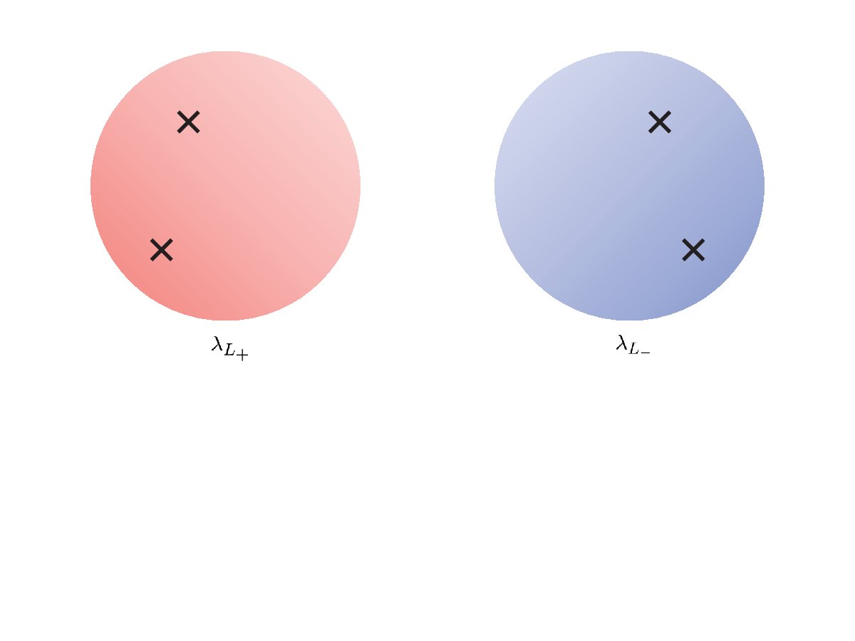
where each of the spectral parameters take the values on a Riemann sphere with two punctures: λL±∈ℂ∪{∞}\lambda_{L_{\pm}}\in{\mathbb{C}}\cup\{\infty\} . The punctures come from the fact that each Lax pair has two poles at λL±=±1\lambda_{L_{\pm}}=\pm 1 , as depicted in Fig. 3.

Refer to caption
Figure 3: Two Riemann spheres with two punctures.

On the other hand, the Lax pair in the right description [See (4.1)] is given by

LtR​(x,λR)=12​[L+R​(x,λR)+L−R​(x,λR)],\displaystyle L^{R}_{t}(x;\lambda_{R})=\frac{1}{2}\left[L^{R}_{+}(x;\lambda_{R})+L^{R}_{-}(x;\lambda_{R})\right]\,,
LxR​(x,λR)=12​[L+R​(x,λR)−L−R​(x,λR)],\displaystyle L^{R}_{x}(x;\lambda_{R})=\frac{1}{2}\left[L^{R}_{+}(x;\lambda_{R})-L^{R}_{-}(x;\lambda_{R})\right]\,,
L±R​(x,λR)=−sinh⁡(α±β)sinh⁡[α±(β+λR)]​[T+​J±−+T−​J±++cosh⁡(α±λR)cosh⁡α​T3​J±3].\displaystyle L^{R}_{\pm}(x;\lambda_{R})=-\frac{\sinh\left(\alpha\pm\beta\right)}{\sinh\left[\alpha\pm(\beta+\lambda_{R})\right]}\left[T^{+}J^{-}_{\pm}+T^{-}J^{+}_{\pm}+\frac{\cosh\left(\alpha\pm\lambda_{R}\right)}{\cosh\alpha}T^{3}J^{3}_{\pm}\right]\,.

The spectral parameter λR\lambda_{R} is periodically identified as

λR∼λR+2​π​i,\displaystyle\lambda_{R}\sim\lambda_{R}+2\pi i\,, (5.1)

and hence it takes the values on a cylinder. Because the right Lax pair is regular in the Re​λR→±∞{\rm Re}\lambda_{R}\to\pm\infty limit, the fundamental domain of spectral parameter can be regarded as a Riemann sphere under the map

λR→zR=eλR.\displaystyle\lambda_{R}\to z_{R}={\rm e}^{\lambda_{R}}\,. (5.2)

It is obvious that the right Lax pair has four poles at

zR=e±α−β,−e±α−β.\displaystyle z_{R}={\rm e}^{\pm\alpha-\beta}\,,~-{\rm e}^{\pm\alpha-\beta}\,. (5.3)

Thus the domain of the spectral parameter zRz_{R} is regarded as a Riemann sphere with four punctures as depicted in Fig. 4§§ § When α\alpha and β\beta are real, the four poles are on the real axis of the zRz_{R}-plane. When α\alpha and β\beta are purely imaginary, the four poles are on the unit circle with the center at the origin. .

Refer to caption
Figure 4: The Riemann sphere with four punctures for α\alpha and β\beta are purely imaginary.

In the following, we show that the Riemann sphere of zRz_{R} is related to a pair of the Riemann spheres of λL±\lambda_{L_{\pm}} .

The reduced right descriptions

As a next step, we introduce the reduced right descriptions. Lax pairs in the reduced right descriptions are obtained from the original right Lax pair through the following isomorphisms of the s​l​(2)sl(2) algebra,

T±→e±λR​T±=e−i​λR​T3​T±​ei​λR​T3\displaystyle T^{\pm}~~\to~~{\rm e}^{\pm\lambda_{R}}T^{\pm}={\rm e}^{-i\lambda_{R}T^{3}}T^{\pm}{\rm e}^{i\lambda_{R}T^{3}} (5.4)
or\displaystyle{\rm or}\quad T±→e∓λR​T±=ei​λR​T3​T±​e−i​λR​T3.\displaystyle T^{\pm}~~\to~~{\rm e}^{\mp\lambda_{R}}T^{\pm}={\rm e}^{i\lambda_{R}T^{3}}T^{\pm}{\rm e}^{-i\lambda_{R}T^{3}}\,. (5.5)

Because T3T^{3} is invariant under the isomorphisms, the generators can be rewritten into

Ta→e∓i​λR​T3​Ta​e±i​λR​T3.\displaystyle T^{a}\to{\rm e}^{\mp i\lambda_{R}T^{3}}T^{a}{\rm e}^{\pm i\lambda_{R}T^{3}}\,. (5.6)

One of the resulting Lax pairs is

L±R+​(x,λR+)\displaystyle L^{R_{+}}_{\pm}(x;\lambda_{R_{+}}) =\displaystyle= −sinh⁡(α±β)sinh⁡[α±(β+λR+)]\displaystyle-\frac{\sinh\left(\alpha\pm\beta\right)}{\sinh\left[\alpha\pm\left(\beta+\lambda_{R_{+}}\right)\right]} (5.7)
×[e+λR+​T+​J±−+e−λR+​T−​J±++cosh⁡(α±λR+)cosh⁡α​T3​J±3].\displaystyle\quad\times\left[{\rm e}^{+\lambda_{R_{+}}}T^{+}J^{-}_{\pm}+{\rm e}^{-\lambda_{R_{+}}}T^{-}J^{+}_{\pm}+\frac{\cosh\left(\alpha\pm\lambda_{R_{+}}\right)}{\cosh\alpha}T^{3}J^{3}_{\pm}\right]\,.

For later convenience, we change the subscript of the spectral parameter from RR to R+R_{+} . This reduced right Lax pair corresponds to the former isomorphism (5.4) . Similarly, the other reduced right Lax pair is defined as

L±R−​(x,λR−)\displaystyle L^{R_{-}}_{\pm}(x;\lambda_{R_{-}}) =\displaystyle= −sinh⁡(α±β)sinh⁡[α±(β+λR−)]\displaystyle-\frac{\sinh\left(\alpha\pm\beta\right)}{\sinh\left[\alpha\pm\left(\beta+\lambda_{R_{-}}\right)\right]} (5.8)
×[e−λR−​T+​J±−+e+λR−​T−​J±++cosh⁡(α±λR−)cosh⁡α​T3​J±3].\displaystyle\quad\times\left[{\rm e}^{-\lambda_{R_{-}}}T^{+}J^{-}_{\pm}+{\rm e}^{+\lambda_{R_{-}}}T^{-}J^{+}_{\pm}+\frac{\cosh\left(\alpha\pm\lambda_{R_{-}}\right)}{\cosh\alpha}T^{3}J^{3}_{\pm}\right]\,.

For this reduced right Lax pair, its spectral parameter is denoted as λR−\lambda_{R_{-}} . This reduced right Lax pair corresponds to the later isomorphism (5.5) .

Note that the domains of the spectral parameters λR±\lambda_{R_{\pm}} have the periodicities,

λR±∼λR±+π​i,\displaystyle\lambda_{R_{\pm}}\sim\lambda_{R_{\pm}}+\pi i\,, (5.9)

and hence the squares of zR±z_{R_{\pm}}

zR±2=e2​λR±\displaystyle z_{R_{\pm}}^{2}={\rm e}^{2\lambda_{R_{\pm}}} (5.10)

live on the Riemann spheres Note that zR±z_{R_{\pm}} and −zR±-z_{R_{\pm}} cannot be distinguished and hence zR±2z_{R_{\pm}}^{2} takes the value on a Riemann sphere.. Each of the reduced right Lax pairs LμR±​(λR±)L^{R_{\pm}}_{\mu}(\lambda_{R_{\pm}}) has two poles in its fundamental domain,

zR±2=e2​α−2​βande−2​α−2​β.\displaystyle z_{R_{\pm}}^{2}={\rm e}^{2\alpha-2\beta}\quad{\rm and}\quad{\rm e}^{-2\alpha-2\beta}\,. (5.11)

As a result, the fundamental domains of zR±2z_{R_{\pm}}^{2} are a pair of Riemann spheres with two punctures.

So far, we have shown that the right description is decomposed to a couple of the reduced right descriptions. The statement we want to show is that each of the Lax pair in the reduced right description is equivalent to each of the Lax pairs in the left description through a gauge transformation with a certain identification of the spectral parameters.

A relation of the spectral parameters

Then the next task is to find out a relation of the spectral parameters in the left and right descriptions. Because both λL±\lambda_{L_{\pm}} and zR±2z_{R_{\pm}}^{2} live on the two-punctured Riemann spheres, they should be related through a Möbius transformation,

zR±2=a​λL±+bc​λL±+d.\displaystyle z_{R_{\pm}}^{2}=\frac{a\lambda_{L_{\pm}}+b}{c\lambda_{L_{\pm}}+d}\,. (5.12)

The constant parameter should be fixed by the pole structure and the correspondence of the expansion points for Yangians.

The first requirement is that the position of the poles should be mapped each other. This condition leads to

e±2​α−2​β=a±bc±d.\displaystyle{\rm e}^{\pm 2\alpha-2\beta}=\frac{a\pm b}{c\pm d}\,. (5.13)

Now we have two possibilities: the pole at zR±2=e2​α−2​βz_{R_{\pm}}^{2}={\rm e}^{2\alpha-2\beta} corresponds to 1) the pole at λL±=1\lambda_{L_{\pm}}=1 , or 2) the pole at λL±=−1\lambda_{L_{\pm}}=-1 . However, we should here take the possibility 1) so that the resulting Möbius transformation reproduces the result in [27] when K=0K=0 .

Then, recall that the Yangian charges Q(n)L±Q^{L_{\pm}}_{(n)} are obtained by expanding the (reduced) right Lax pairs around zR±2=1z_{R_{\pm}}^{2}=1 . From this information, the following relation is obtained,

1=ac.\displaystyle 1=\frac{a}{c}\,. (5.14)

Thus the final result is given by

zR±2=sinh⁡2​α​λL±+cosh⁡2​α−e−2​βsinh⁡2​α​λL±−cosh⁡2​α+e2​β=λL±+K+i​AλL±+K−i​A,\displaystyle z_{R_{\pm}}^{2}=\frac{\sinh 2\alpha\lambda_{L_{\pm}}+\cosh 2\alpha-{\rm e}^{-2\beta}}{\sinh 2\alpha\lambda_{L_{\pm}}-\cosh 2\alpha+{\rm e}^{2\beta}}=\frac{\lambda_{L_{\pm}}+K+iA}{\lambda_{L_{\pm}}+K-iA}\,, (5.15)

or equivalently,

λL±+Ki​A=1tanh⁡λR±.\displaystyle\frac{\lambda_{L_{\pm}}+K}{iA}=\frac{1}{\tanh\lambda_{R_{\pm}}}\,. (5.16)

Here we comment on the connection between the two-punctured λL\lambda_{L}-Riemann spheres and the four-punctured zRz_{R}-Riemann sphere. The relation between zRz_{R} and λL\lambda_{L} is also given by (5.15) :

zR2=λL±+K+i​AλL±+K−i​A.\displaystyle z_{R}^{2}=\frac{\lambda_{L_{\pm}}+K+iA}{\lambda_{L_{\pm}}+K-iA}\,. (5.17)

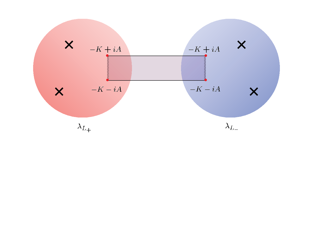
However the interpretation is more involved because −zR-z_{R} is certainly a different from the point zRz_{R} . As a relation between zRz_{R} and λL±\lambda_{L_{\pm}} (not zR2z_{R}^{2} and λL±\lambda_{L_{\pm}} ) , the relation in (5.17) indicates that there exists a cut between λL±=−K+i​A\lambda_{L_{\pm}}=-K+iA and λL±=−K−i​A\lambda_{L_{\pm}}=-K-iA . Two-punctured λL\lambda_{L}-Riemann spheres are connected along the cut and combined into a single Riemann sphere with four punctures. The resulting four-punctured Riemann sphere is depicted in Fig.5.
Refer to caption
Figure 5: Two-punctured λL\lambda_{L}-Riemann spheres are connected along the cut.

The gauge equivalence

We concentrate on showing the gauge equivalence between LμR+​(x,λR+)L^{R_{+}}_{\mu}(x;\lambda_{R_{+}}) and LμL+​(x,λL+)L^{L_{+}}_{\mu}(x;\lambda_{L_{+}}) . The analysis for the case with (-)-subscript is also similar. The gauge transformation is generated by gg and the relation between the spectral parameters is given by

λL++Ki​A=1tanh⁡λR+.\displaystyle\frac{\lambda_{L_{+}}+K}{iA}=\frac{1}{\tanh\lambda_{R_{+}}}\,. (5.18)

First of all, the left Lax pair LμL+​(x,λL+)L^{L_{+}}_{\mu}(x;\lambda_{L_{+}}) can be rewritten as

L±L+​(x,λL+)\displaystyle L^{L_{+}}_{\pm}(x;\lambda_{L_{+}}) (5.19)
=\displaystyle= 11±λL+​g​(J±−2​C​tr​(T3​J±)​T3∓K​J±∓A⁡[J±,T3])​g−1\displaystyle\frac{1}{1\pm\lambda_{L_{+}}}g\left(J_{\pm}-2C{\rm tr}\left(T^{3}J_{\pm}\right)T^{3}\mp KJ_{\pm}\mp A\left[J_{\pm},T^{3}\right]\right)g^{-1}
=\displaystyle= 11±λL+g[T+(1∓K∓iA)J±−+T−(1∓K±iA)J±+\displaystyle\frac{1}{1\pm\lambda_{L_{+}}}g\left[T^{+}\left(1\mp K\mp iA\right)J^{-}_{\pm}+T^{-}\left(1\mp K\pm iA\right)J^{+}_{\pm}\right.
+T3(1+C∓K)J±3]g−1.\displaystyle\hskip 142.26378pt\left.+T^{3}\left(1+C\mp K\right)J^{3}_{\pm}\right]g^{-1}\,.

Then a gauge-transformation of the left Lax pair is given by

[L±L+​(x,λL+)]g\displaystyle\Bigl[L^{L_{+}}_{\pm}(x;\lambda_{L_{+}})\Bigr]^{g} (5.20)
≡\displaystyle\equiv g−1​L±L+​(x,λL+)​g−g−1​∂±g\displaystyle g^{-1}L^{L_{+}}_{\pm}(x;\lambda_{L_{+}})g-g^{-1}\partial_{\pm}g
=\displaystyle= −J±+11±λL+[T+(1∓K∓iA)J±−+T−(1∓K±iA)J±+\displaystyle-J_{\pm}+\frac{1}{1\pm\lambda_{L_{+}}}\left[T^{+}\left(1\mp K\mp iA\right)J^{-}_{\pm}+T^{-}\left(1\mp K\pm iA\right)J^{+}_{\pm}\right.
+T3(1+C∓K)J±3]\displaystyle\hskip 142.26378pt\left.+T^{3}\left(1+C\mp K\right)J^{3}_{\pm}\right]
=\displaystyle= −[λL++K+i​AλL+±1​T+​J±−+λL++K−i​AλL+±1​T−​J±++λL++K∓CλL+±1​T3​J±3].\displaystyle-\left[\frac{\lambda_{L_{+}}+K+iA}{\lambda_{L_{+}}\pm 1}T^{+}J^{-}_{\pm}+\frac{\lambda_{L_{+}}+K-iA}{\lambda_{L_{+}}\pm 1}T^{-}J^{+}_{\pm}+\frac{\lambda_{L_{+}}+K\mp C}{\lambda_{L_{+}}\pm 1}T^{3}J^{3}_{\pm}\right]\,.

Finally, with the relation between the spectral parameters (5.18) , it becomes the reduced right Lax pair:

[L±L+​(x,λL+)]g\displaystyle\Bigl[L^{L_{+}}_{\pm}(x;\lambda_{L_{+}})\Bigr]^{g} (5.21)
=\displaystyle= −sinh⁡(α±β)sinh⁡[α±(β+λR+)]​[e+λR+​T+​J±−+e−λR−​T−​J±++cosh⁡(α±λR+)cosh⁡α​T3​J±3]\displaystyle-\frac{\sinh\left(\alpha\pm\beta\right)}{\sinh\left[\alpha\pm\left(\beta+\lambda_{R_{+}}\right)\right]}\left[{\rm e}^{+\lambda_{R_{+}}}T^{+}J^{-}_{\pm}+{\rm e}^{-\lambda_{R_{-}}}T^{-}J^{+}_{\pm}+\frac{\cosh\left(\alpha\pm\lambda_{R_{+}}\right)}{\cosh\alpha}T^{3}J^{3}_{\pm}\right]
=\displaystyle= L±R+​(x,λR+).\displaystyle L^{R_{+}}_{\pm}(x;\lambda_{R_{+}})\,.

Similarly, with the spectral-parameter relation

λL−+Ki​A=1tanh⁡λR−,\displaystyle\frac{\lambda_{L_{-}}+K}{iA}=\frac{1}{\tanh\lambda_{R_{-}}}\,, (5.22)

we can show the gauge equivalence between the other left Lax pair LμL−​(x,λL−)L^{L_{-}}_{\mu}(x;\lambda_{L_{-}}) and the other reduced right Lax pair LμR​(x,λR−)L^{R\-}_{\mu}(x;\lambda_{R_{-}}) :

[L±L−​(x,λL−)]g=L±R−​(x,λR−).\displaystyle\Bigl[L^{L_{-}}_{\pm}(x;\lambda_{L_{-}})\Bigr]^{g}=L^{R_{-}}_{\pm}(x;\lambda_{R_{-}})\,. (5.23)

Summary

Let us summarize the results obtained so far. The two reduced right Lax pairs LμR±​(x,λR±)L^{R_{\pm}}_{\mu}(x;\lambda_{R_{\pm}}) have been introduced. Then they are obtained from the right Lax pair through the s​l​(2)sl(2) isomorphisms,

Ta→e∓i​λR​T3​Ta​e±i​λR​T3.\displaystyle T^{a}\to{\rm e}^{\mp i\lambda_{R}T^{3}}T^{a}{\rm e}^{\pm i\lambda_{R}T^{3}}\,. (5.24)

The reduced right Lax pairs LμR±​(x,λR±)L^{R_{\pm}}_{\mu}(x;\lambda_{R_{\pm}}) are related to the left Lax pairs LμL±​(x,λL±)L^{L_{\pm}}_{\mu}(x;\lambda_{L_{\pm}}) through the gauge transformation generated by gg ,

[LμL±​(x,λL±)]g=LμR±​(x,λR±),\displaystyle\Bigl[L^{L_{\pm}}_{\mu}(x;\lambda_{L_{\pm}})\Bigr]^{g}=L^{R_{\pm}}_{\mu}(x;\lambda_{R_{\pm}})\,, (5.25)

under the relations between the spectral parameters

λL±+Ki​A=1tanh⁡λR±.\displaystyle\frac{\lambda_{L_{\pm}}+K}{iA}=\frac{1}{\tanh\lambda_{R_{\pm}}}\,. (5.26)

So far we have shown that UL±​(λL±)U^{L_{\pm}}(\lambda_{L_{\pm}}) are gauge-equivalent to UR±​(λR±)U^{R_{\pm}}(\lambda_{R_{\pm}}) and hence the charges for the deformed Uq​(s​u​(2)^R)U_{q}(\widehat{su(2)}_{\rm R}) can also be obtained from UL±​(λL±)U^{L_{\pm}}(\lambda_{L_{\pm}}) . One can read off the expansion points from the relation (5.26) and the fact that the expansion points for UR±​(λR±)U^{R_{\pm}}(\lambda_{R_{\pm}}) are zR±=0z_{R_{\pm}}=0 and zR±=∞z_{R_{\pm}}=\infty . Thus the charges for the deformed Uq​(s​u​(2)^R)U_{q}(\widehat{su(2)}_{\rm R}) are obtained by expanding UL±​(λL±)U^{L_{\pm}}(\lambda_{L_{\pm}}) with respect to λL±\lambda_{L_{\pm}} around λL±=−K−i​A\lambda_{L_{\pm}}=-K-iA and λL±=−K+i​A\lambda_{L_{\pm}}=-K+iA . The locations of poles and the expansion points for the deformed Uq​(s​u​(2)^R)U_{q}(\widehat{su(2)}_{\rm R}) and 𝒴⁡(s​u​(2)L){\mathcal{Y}}(su(2)_{\rm L}) are summarized in Tab. 1 .

Charges ∖\setminus Monodromies UR±​(λR±)\qquad U^{R_{\pm}}(\lambda_{R_{\pm}})\qquad UL±​(λL±)\qquad U^{L_{\pm}}(\lambda_{L_{\pm}})\qquad
Q(0)R,3,Q(1)R,+,Q~(1)R,−Q^{R,3}_{(0)}\,,Q^{R,+}_{(1)}\,,\widetilde{Q}^{R,-}_{(1)} 00 −K−i​A-K-iA
Q(0)R,3,Q(1)R,−,Q~(1)R,+Q^{R,3}_{(0)}\,,Q^{R,-}_{(1)}\,,\widetilde{Q}^{R,+}_{(1)} ∞\infty −K+i​A-K+iA
Q(0)L,a,Q(1)L,aQ^{L,a}_{(0)}\,,Q^{L,a}_{(1)} 11 ∞\infty
local charges e±2​α−2​β{\rm e}^{\pm 2\alpha-2\beta} ±1\pm 1
Table 1: The conserved charges and the expansion points of monodromy matrices are listed. The expansion points of UR±​(λR±)U^{R_{\pm}}(\lambda_{R_{\pm}}) are described in terms of zR±2z_{R_{\pm}}^{2} .

The gauge transformation of the r/sr/s-matrices

The rr/ss-matrices for the reduced right Lax pairs can be obtained from the rr/ss-matrices for the left Lax pairs. Recall the gauge-transformation laws of the rr/ss-matrices,

(r+s)R±​(λR±,μR±)​δ​(x−y)\displaystyle(r+s)^{R_{\pm}}(\lambda_{R_{\pm}},\mu_{R_{\pm}})\delta(x-y) (5.28)
=\displaystyle= g−1​(x)⊗g−1​(y)\displaystyle g^{-1}(x)\otimes g^{-1}(y)
×[(r+s)L±(λL±,μL±)δ(x−y)−{LxL±(x;λL±),⊗g(y)}P1⊗g−1(y)]\displaystyle\times\Biggl[(r+s)^{L_{\pm}}(\lambda_{L_{\pm}},\mu_{L_{\pm}})\delta(x-y)-\Bigl\{L^{L_{\pm}}_{x}(x;\lambda_{L_{\pm}})\stackrel{{\scriptstyle\otimes}}{{,}}g(y)\Bigr\}_{\rm P}1\otimes g^{-1}(y)\Biggr]
×g⁡(x)⊗g⁡(y),\displaystyle\times g(x)\otimes g(y)\,,
(r−s)R±​(λR±,μR±)​δ​(x−y)\displaystyle(r-s)^{R_{\pm}}(\lambda_{R_{\pm}},\mu_{R_{\pm}})\delta(x-y)
=\displaystyle= g−1​(x)⊗g−1​(y)\displaystyle g^{-1}(x)\otimes g^{-1}(y)
×[(r−s)L±(λL±,μL±)δ(x−y)−{g(x),⊗LxL±(y;μL±)}P1⊗g−1(y)]\displaystyle\times\Biggl[(r-s)^{L_{\pm}}(\lambda_{L_{\pm}},\mu_{L_{\pm}})\delta(x-y)-\Bigl\{g(x)\stackrel{{\scriptstyle\otimes}}{{,}}L^{L_{\pm}}_{x}(y;\mu_{L_{\pm}})\Bigr\}_{\rm P}1\otimes g^{-1}(y)\Biggr]
×g⁡(x)⊗g⁡(y).\displaystyle\times g(x)\otimes g(y)\,.

Thus the Poisson brackets

{LxL±(x;λL)⊗,g(y)}P1⊗g−1(y)\displaystyle\Bigl\{L^{L_{\pm}}_{x}(x;\lambda_{L})\otimes,g(y)\Bigr\}_{\rm P}1\otimes g^{-1}(y) (5.29)
=\displaystyle= −11−λL2{(−λL−K1+C)(T−⊗T++T+⊗T−+T3⊗T3)\displaystyle\frac{-1}{1-\lambda_{L}^{2}}\left\{\left(-\lambda_{L}-\frac{K}{1+C}\right)\left(T^{-}\otimes T^{+}+T^{+}\otimes T^{-}+T^{3}\otimes T^{3}\right)\right.
±A⁡[T−⊗T++T+⊗T−+T3⊗T3,1⊗g​T3​g−1​(y)]\displaystyle\qquad\qquad\left.\pm A\left[T^{-}\otimes T^{+}+T^{+}\otimes T^{-}+T^{3}\otimes T^{3},1\otimes gT^{3}g^{-1}(y)\right]\right.
+C​K1+C[[T−⊗T++T+⊗T−+T3⊗T3,1⊗gT3g−1(y)],1⊗gT3g−1(y)]}\displaystyle\qquad\qquad\left.+\frac{CK}{1+C}\left[\left[T^{-}\otimes T^{+}+T^{+}\otimes T^{-}+T^{3}\otimes T^{3},1\otimes gT^{3}g^{-1}(y)\right],1\otimes gT^{3}g^{-1}(y)\right]\right\}
×δ⁡(x−y),\displaystyle\qquad\times\delta(x-y)\,,
{g(x)⊗,LxL±(y;μL)}Pg−1(x)⊗1\displaystyle\Bigl\{g(x)\otimes,L^{L_{\pm}}_{x}(y;\mu_{L})\Bigr\}_{\rm P}g^{-1}(x)\otimes 1 (5.30)
=\displaystyle= 11−μL2{(−μL−K1+C)(T−⊗T++T+⊗T−+T3⊗T3)\displaystyle\frac{1}{1-\mu_{L}^{2}}\left\{\left(-\mu_{L}-\frac{K}{1+C}\right)\left(T^{-}\otimes T^{+}+T^{+}\otimes T^{-}+T^{3}\otimes T^{3}\right)\right.
±A⁡[T−⊗T++T+⊗T−+T3⊗T3,g​T3​g−1​(x)⊗1]\displaystyle\qquad\qquad\left.\pm A\left[T^{-}\otimes T^{+}+T^{+}\otimes T^{-}+T^{3}\otimes T^{3},gT^{3}g^{-1}(x)\otimes 1\right]\right.
+C​K1+C[[T−⊗T++T+⊗T−+T3⊗T3,gT3g−1(x)⊗1],gT3g−1(x)⊗1]}\displaystyle\qquad\qquad\left.+\frac{CK}{1+C}\left[\left[T^{-}\otimes T^{+}+T^{+}\otimes T^{-}+T^{3}\otimes T^{3},gT^{3}g^{-1}(x)\otimes 1\right],gT^{3}g^{-1}(x)\otimes 1\right]\right\}
×δ⁡(x−y),\displaystyle\qquad\times\delta(x-y)\,,

are needed to compute the rr/ss-matrices for the reduced right Lax pair.

With the explicit expression of the rr/ss-matrices for the left Lax pairs (3.13) , the relation (5.29) and the maps between spectral parameters (5.26) , we can evaluate the right hand side of (5.28) as

(r+s)R±​(λR±,μR±)​δ​(x−y)\displaystyle(r+s)^{R_{\pm}}(\lambda_{R_{\pm}},\mu_{R_{\pm}})\delta(x-y) (5.31)
=\displaystyle= 1sinh⁡(λR±−μR±)​sinh⁡2​α​sinh2⁡λR±2​sinh⁡(α+β+λR±)​sinh⁡(α−β−λR±)\displaystyle\frac{1}{\sinh(\lambda_{R_{\pm}}-\mu_{R_{\pm}})}\frac{\sinh 2\alpha\sinh^{2}\lambda_{R_{\pm}}}{2\sinh(\alpha+\beta+\lambda_{R_{\pm}})\sinh(\alpha-\beta-\lambda_{R_{\pm}})}
×{[cosh(λR±−μR±)−tanhβsinh(λR±−μR±)]T3⊗T3\displaystyle\times\Biggl\{\left[\cosh(\lambda_{R_{\pm}}-\mu_{R_{\pm}})-\tanh\beta\sinh(\lambda_{R_{\pm}}-\mu_{R_{\pm}})\right]T^{3}\otimes T^{3}
+e±(λR±−μR±)T−⊗T++e∓(λR±−μR±)T+⊗T−}δ(x−y).\displaystyle\qquad+{\rm e}^{\pm(\lambda_{R_{\pm}}-\mu_{R_{\pm}})}T^{-}\otimes T^{+}+{\rm e}^{\mp(\lambda_{R_{\pm}}-\mu_{R_{\pm}})}T^{+}\otimes T^{-}\Biggr\}\delta(x-y)\,.

Similarly, the following can be obtained

(r−s)R±​(λR±,μR±)​δ​(x−y)\displaystyle(r-s)^{R_{\pm}}(\lambda_{R_{\pm}},\mu_{R_{\pm}})\delta(x-y) (5.32)
=\displaystyle= 1sinh⁡(λR±−μR±)​sinh⁡2​α​sinh2⁡μR±2​sinh⁡(α+β+μR±)​sinh⁡(α−β−μR±)\displaystyle\frac{1}{\sinh(\lambda_{R_{\pm}}-\mu_{R_{\pm}})}\frac{\sinh 2\alpha\sinh^{2}\mu_{R_{\pm}}}{2\sinh(\alpha+\beta+\mu_{R_{\pm}})\sinh(\alpha-\beta-\mu_{R_{\pm}})}
×{[cosh(λR±−μR±)+tanhβsinh(λR±−μR±)]T3⊗T3\displaystyle\times\Biggl\{\left[\cosh(\lambda_{R_{\pm}}-\mu_{R_{\pm}})+\tanh\beta\sinh(\lambda_{R_{\pm}}-\mu_{R_{\pm}})\right]T^{3}\otimes T^{3}
+e±(λR±−μR±)T−⊗T++e∓(λR±−μR±)T+⊗T−}δ(x−y).\displaystyle\qquad+{\rm e}^{\pm(\lambda_{R_{\pm}}-\mu_{R_{\pm}})}T^{-}\otimes T^{+}+{\rm e}^{\mp(\lambda_{R_{\pm}}-\mu_{R_{\pm}})}T^{+}\otimes T^{-}\Biggr\}\delta(x-y)\,.

Thus the resulting rr/ss-matrices for the reduced right Lax pairs are

rR±​(λR±,μR±)\displaystyle r^{R_{\pm}}(\lambda_{R_{\pm}},\mu_{R_{\pm}}) =\displaystyle= hα,βR​(λR±)+hα,βR​(μR±)2​sinh⁡(λR±−μR±)\displaystyle\frac{h^{R}_{\alpha,\beta}(\lambda_{R_{\pm}})+h^{R}_{\alpha,\beta}(\mu_{R_{\pm}})}{2\sinh(\lambda_{R_{\pm}}-\mu_{R_{\pm}})}
×[e±(λR±−μR±)T−⊗T++e∓(λR±−μR±)T+⊗T−\displaystyle\times\left[{\rm e}^{\pm(\lambda_{R_{\pm}}-\mu_{R_{\pm}})}T^{-}\otimes T^{+}+{\rm e}^{\mp(\lambda_{R_{\pm}}-\mu_{R_{\pm}})}T^{+}\otimes T^{-}\right.
+cosh(λR±−μR±)T3⊗T3]\displaystyle\qquad\left.+\cosh(\lambda_{R_{\pm}}-\mu_{R_{\pm}})T^{3}\otimes T^{3}\right]
−(hα,βR​(λR±)−hα,βR​(μR±))2tanhβT3⊗T3,\displaystyle-\frac{\left(h^{R}_{\alpha,\beta}(\lambda_{R_{\pm}})-h^{R}_{\alpha,\beta}(\mu_{R_{\pm}})\right)}{2}\tanh\beta T^{3}\otimes T^{3}\,,
sR±​(λR±,μR±)\displaystyle s^{R_{\pm}}(\lambda_{R_{\pm}},\mu_{R_{\pm}}) =\displaystyle= hα,βR​(λR±)−hα,βR​(μR±)2​sinh⁡(λR±−μR±)\displaystyle\frac{h^{R}_{\alpha,\beta}(\lambda_{R_{\pm}})-h^{R}_{\alpha,\beta}(\mu_{R_{\pm}})}{2\sinh(\lambda_{R_{\pm}}-\mu_{R_{\pm}})}
×[e±(λR±−μR±)T−⊗T++e∓(λR±−μR±)T+⊗T−\displaystyle\times\left[{\rm e}^{\pm(\lambda_{R_{\pm}}-\mu_{R_{\pm}})}T^{-}\otimes T^{+}+{\rm e}^{\mp(\lambda_{R_{\pm}}-\mu_{R_{\pm}})}T^{+}\otimes T^{-}\right.
+cosh(λR±−μR±)T3⊗T3]\displaystyle\qquad\left.+\cosh(\lambda_{R_{\pm}}-\mu_{R_{\pm}})T^{3}\otimes T^{3}\right]
−(hα,βR​(λR±)+hα,βR​(μR±))2tanhβT3⊗T3.\displaystyle-\frac{\left(h^{R}_{\alpha,\beta}(\lambda_{R_{\pm}})+h^{R}_{\alpha,\beta}(\mu_{R_{\pm}})\right)}{2}\tanh\beta T^{3}\otimes T^{3}\,.

The rr/ss-matrices for the right Lax pair (4.38) are obtained from these rr/ss-matrices for the reduced right Lax pairs by taking the isomorphism of s​l​(2)sl(2) (5.24) into account.

6 The degenerate limits

So far, it has been shown that U​(1)RU(1)_{\rm R} is enhanced to qq-deformed s​u​(2)Rsu(2)_{\rm R} . Then let us argue the q→1q\to 1 limit in which qq-deformed s​u​(2)Rsu(2)_{\rm R} degenerates to the original s​u​(2)Rsu(2)_{\rm R} .

In fact, there are two kinds of the q→1q\to 1 limit, which are referred to as the degenerate limits. Since the qq-parameter is written as q=eγq={\rm e}^{\gamma} , the limits are specified by the condition, γ=0\gamma=0 . From (4.19) , this condition is equivalent to

α=0orα=π​i2.\displaystyle\alpha=0\qquad{\rm or}\qquad\alpha=\frac{\pi i}{2}\,. (6.1)

In the following, we will argue each of the limits.

6.1 α=0\alpha=0

We begin with the α→0\alpha\to 0 limit. Recall the relation between the original parameters (C,K)(C,K) and the parameters (α,β)(\alpha,\beta) , (4.5) . Due to the relation and the finiteness of the original parameters, the condition α=0\alpha=0 requires the condition β=0\beta=0 .

Let us rescale α\alpha and β\beta as

α→ϵ​α,β→ϵ​β,\displaystyle\alpha\to\epsilon\,\alpha\,,\qquad\beta\to\epsilon\,\beta\,, (6.2)

and take the ϵ→0\epsilon\to 0 limit. Then the relation (4.5) is reduced to the following:

K=βα,C=0,A=0.\displaystyle K=\frac{\beta}{\alpha}\,,\qquad C=0\,,\qquad A=0\,. (6.3)

Thus this limit reproduces the undeformed S​U​(2)SU(2) WZNW models.

Next we consider the limit for the right Lax pair. Let us perform the redefinition of spectral parameter,

λR→ϵ​α​λR−ϵ​β,\displaystyle\lambda_{R}\to\epsilon\alpha\lambda_{R}-\epsilon\beta\,, (6.4)

and take the ϵ→0\epsilon\to 0 limit. Then the Lax pair is evaluated as

L±R​(x,λR)=−1±K1±λR​[T+​J±−+T−​J±++T3​J±3].\displaystyle L^{R}_{\pm}(x;\lambda_{R})=-\frac{1\pm K}{1\pm\lambda_{R}}\left[T^{+}J^{-}_{\pm}+T^{-}J^{+}_{\pm}+T^{3}J^{3}_{\pm}\right]\,. (6.5)

The same procedure gives rise to the rr/ss-matrices,

rR​(λR,μR)\displaystyle r^{R}(\lambda_{R},\mu_{R}) =\displaystyle= h0R​(λR)+h0R​(μR)2​(λR−μR)​[T−⊗T++T+⊗T−+T3⊗T3],\displaystyle\frac{h^{R}_{0}(\lambda_{R})+h^{R}_{0}(\mu_{R})}{2(\lambda_{R}-\mu_{R})}\left[T^{-}\otimes T^{+}+T^{+}\otimes T^{-}+T^{3}\otimes T^{3}\right]\,, (6.6)
sR​(λR,μR)\displaystyle s^{R}(\lambda_{R},\mu_{R}) =\displaystyle= h0R​(λR)−h0R​(μR)2​(λR−μR)​[T−⊗T++T+⊗T−+T3⊗T3].\displaystyle\frac{h^{R}_{0}(\lambda_{R})-h^{R}_{0}(\mu_{R})}{2(\lambda_{R}-\mu_{R})}\left[T^{-}\otimes T^{+}+T^{+}\otimes T^{-}+T^{3}\otimes T^{3}\right]\,.

Here the function h0R​(λ)h^{R}_{0}(\lambda) is given by

h0R​(λ)=(λ−K)21−λ2.\displaystyle h^{R}_{0}(\lambda)=\frac{\left(\lambda-K\right)^{2}}{1-\lambda^{2}}\,. (6.7)

Since γ±=0\gamma^{\pm}=0 and A=0A=0 , two sets of non-local currents jμR,±j^{R,\pm}_{\mu} and j~μR,±\widetilde{j}^{R,\pm}_{\mu} degenerate into

jμR,±=j~μR,±=−(Jμ±+K​ϵμ​ν​J±,ν)≡𝒥μR,±.\displaystyle j^{R,\pm}_{\mu}=\widetilde{j}^{R,\pm}_{\mu}=-\left(J^{\pm}_{\mu}+K\epsilon_{\mu\nu}J^{\pm,\nu}\right)\equiv{\mathcal{J}}^{R,\pm}_{\mu}\,. (6.8)

For later convenience, let us introduce the following matrix valued conserved current:

𝒥μR=T+​𝒥μR,−+T−​𝒥μR,++T3​𝒥μR,3,\displaystyle{\mathcal{J}}^{R}_{\mu}=T^{+}{\mathcal{J}}^{R,-}_{\mu}+T^{-}{\mathcal{J}}^{R,+}_{\mu}+T^{3}{\mathcal{J}}^{R,3}_{\mu}\,, (6.9)

where the T3T^{3} component 𝒥μR,3{\mathcal{J}}^{R,3}_{\mu} is defined as

𝒥μR,3≡jμR,3=−(Jμ3+K​ϵμ​ν​J3,ν).\displaystyle{\mathcal{J}}^{R,3}_{\mu}\equiv j^{R,3}_{\mu}=-\left(J^{3}_{\mu}+K\epsilon_{\mu\nu}J^{3,\nu}\right)\,. (6.10)

It is an easy task to show that this conserved current satisfies the flatness condition:

ϵμ​ν​(∂μ𝒥νR−𝒥μR​𝒥νR)=0,\displaystyle\epsilon^{\mu\nu}\left(\partial_{\mu}{\mathcal{J}}^{R}_{\nu}-{\mathcal{J}}^{R}_{\mu}{\mathcal{J}}^{R}_{\nu}\right)=0\,, (6.11)

and the right Lax pair can be written in terms of the conserved current 𝒥μR{\mathcal{J}}^{R}_{\mu} as

L±R​(x,λR)=𝒥±R1±λR.\displaystyle L^{R}_{\pm}(x;\lambda_{R})=\frac{{\mathcal{J}}^{R}_{\pm}}{1\pm\lambda_{R}}\,. (6.12)

Then it is possible to construct an infinite number of conserved charges from 𝒥μR{\mathcal{J}}^{R}_{\mu} , by following the BIZZ construction [8]:

𝒴(0)R,a\displaystyle{\mathcal{Y}}^{R,a}_{(0)} =\displaystyle= ∫−∞∞d​x​𝒥tR,a​(x),\displaystyle\int^{\infty}_{-\infty}\!\!\!dx~{\mathcal{J}}^{R,a}_{t}(x)\,, (6.13)
𝒴(1)R,a\displaystyle{\mathcal{Y}}^{R,a}_{(1)} =\displaystyle= 14​∫−∞∞d​x​∫−∞∞d​y​εb​ca​ϵ​(x−y)​𝒥tR.b​(x)​𝒥tR.c​(y)−∫−∞∞d​x​𝒥xR.a​(x),\displaystyle\frac{1}{4}\int^{\infty}_{-\infty}\!\!\!dx\int^{\infty}_{-\infty}\!\!\!dy~\varepsilon^{a}_{~bc}\epsilon(x-y){\mathcal{J}}^{R.b}_{t}(x){\mathcal{J}}^{R.c}_{t}(y)-\int^{\infty}_{-\infty}\!\!\!dx~{\mathcal{J}}^{R.a}_{x}(x)\,,
⋮\displaystyle\hskip 85.35826pt\vdots

The current algebra for 𝒥μR,a{\mathcal{J}}^{R,a}_{\mu} is given by

{𝒥tR,a​(x),𝒥tR,b​(y)}P\displaystyle\Bigl\{{\mathcal{J}}^{R,a}_{t}(x),{\mathcal{J}}^{R,b}_{t}(y)\Bigr\}_{\rm P} =\displaystyle= εca​b​𝒥tR,c​(x)+2​K​δa​b​∂xδ⁡(x−y),\displaystyle\varepsilon^{ab}_{~~c}{\mathcal{J}}^{R,c}_{t}(x)+2K\delta^{ab}\partial_{x}\delta(x-y)\,, (6.14)
{𝒥tR,a​(x),𝒥xR,b​(y)}P\displaystyle\Bigl\{{\mathcal{J}}^{R,a}_{t}(x),{\mathcal{J}}^{R,b}_{x}(y)\Bigr\}_{\rm P} =\displaystyle= εca​b​𝒥xR,c​(x)+(1+K2)​δa​b​∂xδ⁡(x−y),\displaystyle\varepsilon^{ab}_{~~c}{\mathcal{J}}^{R,c}_{x}(x)+\left(1+K^{2}\right)\delta^{ab}\partial_{x}\delta(x-y)\,,
{𝒥xR,a​(x),𝒥xR,b​(y)}P\displaystyle\Bigl\{{\mathcal{J}}^{R,a}_{x}(x),{\mathcal{J}}^{R,b}_{x}(y)\Bigr\}_{\rm P} =\displaystyle= −K2​εca​b​𝒥tR,c​(x)+2​K​εca​b​𝒥xR,c​(x)​δ​(x−y)\displaystyle-K^{2}\varepsilon^{ab}_{~~c}{\mathcal{J}}^{R,c}_{t}(x)+2K\varepsilon^{ab}_{~~c}{\mathcal{J}}^{R,c}_{x}(x)\delta(x-y)
+2Kδa​b∂xδ(x−y).\displaystyle+2K\delta^{ab}\partial_{x}\delta(x-y)\,.

With this current algebra, one can show that the algebra formed by a set of 𝒴(n)R{\mathcal{Y}}^{R}_{(n)} is Yangian 𝒴⁡(s​u​(2)L){\mathcal{Y}}(su(2)_{\rm L}) with an appropriate regularization of non-ultra local terms.

6.2 α=π​i/2\alpha=\pi i/2

The other degenerate limit is next considered. Again, due to the relation (4.5) and the finiteness of (C,K)(C,K) , the condition α=π​i/2\alpha=\pi i/2 implies that β=π​i/2\beta=\pi i/2 . So it is useful to redefine α\alpha and β\beta as

α→π​i2+ϵ​α,β→π​i2+ϵ​β.\displaystyle\alpha\quad\to\quad\frac{\pi i}{2}+\epsilon\,\alpha\,,\qquad\beta\quad\to\quad\frac{\pi i}{2}+\epsilon\,\beta\,. (6.15)

The ϵ→0\epsilon\to 0 limit with the redefinition leads to the following relations,

K=βα,C=β2α2−1,A=0.\displaystyle K=\frac{\beta}{\alpha}\,,\qquad C=\frac{\beta^{2}}{\alpha^{2}}-1\,,\qquad A=0\,. (6.16)

This limit describes the points specified by C=K2−1C=K^{2}-1 . As in the case with α=0\alpha=0 , the coefficient of the improvement term vanishes, A=0A=0 . At the points, the effect of the squashing parameter CC is canceled by the Wess-Zumino term. As a result, the right description becomes isotropic even though the metric of target space is deformed.

To see the right Lax pair at the points, the spectral parameter should be redefined as

λR→ϵ​α​λR−ϵ​β.\displaystyle\lambda_{R}\quad\to\quad\epsilon\,\alpha\,\lambda_{R}-\epsilon\,\beta\,. (6.17)

Then the ϵ→0\epsilon\to 0 limit leads to the following expression of the Lax pair,

L±R​(x,λR)=−1±K1±λR​[T+​J±−+T−​J±++(1∓K±λR)​T3​J±3].\displaystyle L^{R}_{\pm}(x;\lambda_{R})=-\frac{1\pm K}{1\pm\lambda_{R}}\left[T^{+}J^{-}_{\pm}+T^{-}J^{+}_{\pm}+\left(1\mp K\pm\lambda_{R}\right)T^{3}J^{3}_{\pm}\right]\,. (6.18)

Similarly, the rr/ss-matrices are obtained as

rR​(λR,μR)\displaystyle r^{R}(\lambda_{R},\mu_{R}) =\displaystyle= hπ​i/2R​(λR)+hπ​i/2R​(μR)2​(λR−μR)​[T−⊗T++T+⊗T−+T3⊗T3]\displaystyle\frac{h^{R}_{\pi i/2}(\lambda_{R})+h^{R}_{\pi i/2}(\mu_{R})}{2(\lambda_{R}-\mu_{R})}\left[T^{-}\otimes T^{+}+T^{+}\otimes T^{-}+T^{3}\otimes T^{3}\right] (6.19)
−hπ​i/2R​(λR)−hπ​i/2R​(μR)2​KT3⊗T3,\displaystyle-\frac{h^{R}_{\pi i/2}(\lambda_{R})-h^{R}_{\pi i/2}(\mu_{R})}{2K}T^{3}\otimes T^{3}\,,
sR​(λR,μR)\displaystyle s^{R}(\lambda_{R},\mu_{R}) =\displaystyle= hπ​i/2R​(λR)−hπ​i/2R​(μR)2​(λR−μR)​[T−⊗T++T+⊗T−+T3⊗T3]\displaystyle\frac{h^{R}_{\pi i/2}(\lambda_{R})-h^{R}_{\pi i/2}(\mu_{R})}{2(\lambda_{R}-\mu_{R})}\left[T^{-}\otimes T^{+}+T^{+}\otimes T^{-}+T^{3}\otimes T^{3}\right]
−hπ​i/2R​(λR)+hπ​i/2R​(μR)2​KT3⊗T3,\displaystyle-\frac{h^{R}_{\pi i/2}(\lambda_{R})+h^{R}_{\pi i/2}(\mu_{R})}{2K}T^{3}\otimes T^{3}\,,

where the function hπ​i/2R​(λ)h^{R}_{\pi i/2}(\lambda) is defined as

hπ​i/2R​(λ)≡(λ−K)21−λ2.\displaystyle h^{R}_{\pi i/2}(\lambda)\equiv\frac{\left(\lambda-K\right)^{2}}{1-\lambda^{2}}\,. (6.20)

In this limit, the following relations are satisfied,

γ±=−γ∓=±i/K,A=0.\gamma^{\pm}=-\gamma^{\mp}=\pm i/K\,,\qquad A=0\,.

Then j~μR,±\widetilde{j}^{R,\pm}_{\mu} coincide with jμR,±j^{R,\pm}_{\mu} as

jμR,±=j~μR,±=−e±iχ/K(J±+Kϵμ​νJ±,ν)≡𝒥μR,±.\displaystyle j_{\mu}^{R,\pm}=\widetilde{j}^{R,\pm}_{\mu}=-{\rm e}^{\pm i\chi/K}\left(J^{\pm}+K\epsilon_{\mu\nu}J^{\pm,\nu}\right)\equiv{\mathcal{J}}^{R,\pm}_{\mu}\,. (6.21)

Note that 𝒥μR,±{\mathcal{J}}^{R,\pm}_{\mu} remain non-local currents, in contrast to the α=0\alpha=0 case. It is useful to define a matrix valued conserved current as

𝒥μR=T+​𝒥μR,−+T−​𝒥μR,++T3​𝒥μR,3,\displaystyle{\mathcal{J}}^{R}_{\mu}=T^{+}{\mathcal{J}}^{R,-}_{\mu}+T^{-}{\mathcal{J}}^{R,+}_{\mu}+T^{3}{\mathcal{J}}^{R,3}_{\mu}\,, (6.22)

where the T3T^{3} component 𝒥μR,3{\mathcal{J}}^{R,3}_{\mu} is defined as

𝒥μR,3≡−jμR,3=(K2​Jμ3+K​ϵμ​ν​J3,ν).\displaystyle{\mathcal{J}}^{R,3}_{\mu}\equiv-j^{R,3}_{\mu}=\left(K^{2}J^{3}_{\mu}+K\epsilon_{\mu\nu}J^{3,\nu}\right)\,. (6.23)

Here the sign of jμR,3j^{R,3}_{\mu} is flipped for later convenience. Although 𝒥μR{\mathcal{J}}^{R}_{\mu} is non-local, it satisfies the flatness condition,

ϵμ​ν​(∂μ𝒥νR−𝒥μR​𝒥νR)=0.\displaystyle\epsilon^{\mu\nu}\left(\partial_{\mu}{\mathcal{J}}^{R}_{\nu}-{\mathcal{J}}^{R}_{\mu}{\mathcal{J}}^{R}_{\nu}\right)=0\,. (6.24)

Thus an infinite number of conserved charges can be constructed from 𝒥μR{\mathcal{J}}^{R}_{\mu} like

𝒴(0)R,a\displaystyle{\mathcal{Y}}^{R,a}_{(0)} =\displaystyle= ∫−∞∞d​x​𝒥tR,a​(x),\displaystyle\int^{\infty}_{-\infty}\!\!\!dx~{\mathcal{J}}^{R,a}_{t}(x)\,, (6.25)
𝒴(1)R,a\displaystyle{\mathcal{Y}}^{R,a}_{(1)} =\displaystyle= 14​∫−∞∞d​x​∫−∞∞d​y​εb​ca​ϵ​(x−y)​𝒥tR.b​(x)​𝒥tR.c​(y)−∫−∞∞d​x​𝒥xR.a​(x),\displaystyle\frac{1}{4}\int^{\infty}_{-\infty}\!\!\!dx\int^{\infty}_{-\infty}\!\!\!dy~\varepsilon^{a}_{~bc}\epsilon(x-y){\mathcal{J}}^{R.b}_{t}(x){\mathcal{J}}^{R.c}_{t}(y)-\int^{\infty}_{-\infty}\!\!\!dx~{\mathcal{J}}^{R.a}_{x}(x)\,,
⋮\displaystyle\hskip 85.35826pt\vdots

Again, the higher-level charges 𝒴(n≥2)R{\mathcal{Y}}^{R}_{(n\geq 2)} are obtained recursively by the BIZZ procedure [8].

In addition, another Lax pair can be obtained from the flat current 𝒥μR{\mathcal{J}}^{R}_{\mu} as

ℒ±R​(λR)=𝒥±R1±λR,\displaystyle{\mathcal{L}}^{R}_{\pm}(\lambda_{R})=\frac{{\mathcal{J}}^{R}_{\pm}}{1\pm\lambda_{R}}\,, (6.26)

where we use the same spectral parameter λR\lambda_{R} , for later convenience. This Lax pair is non-local and hence it is different from the Lax pair (6.18) . However there exists a gauge transformation which connect the non-local Lax pair (6.26) to the right Lax pair (6.18) .

Let us find an appropriate gauge function∥∥ ∥ The strategy is similar to the one to consider the Jordanian twists in the Schrödinger sigma models [29].. An important observation is that, at λR=∞\lambda_{R}=\infty , the right Lax pair (6.18) does not vanish but approaches to a finite quantity as follows:

L±R(λR=∞)=−T3(1±K)J±3=−T3∂±[χK].\displaystyle L^{R}_{\pm}(\lambda_{R}=\infty)=-T^{3}(1\pm K)J^{3}_{\pm}=-T^{3}\partial_{\pm}\left[\frac{\chi}{K}\right]\,. (6.27)

The gauge transformation must be chosen to eliminate this finite part because the non-local Lax pair (6.26) vanishes at λR=∞\lambda_{R}=\infty . Thus the gauge transformation is generated by

F⁡(x)=e−T3​χ⁡(x)K.\displaystyle F(x)={\rm e}^{-T^{3}\frac{\chi(x)}{K}}\,. (6.28)

Note that a constant S​U​(2)SU(2) element may be multiplied from the right and thus the function F⁡(x)F(x) is not determined uniquely. However, the choice in (6.28) is appropriate to relate the right Lax pair (6.18) to the non-local Lax pair (6.26) , as we will see just below.

By performing a non-local gauge transformation generated by F⁡(x)F(x) in (6.28) , the right Lax pair (6.18) can be rewritten as

L±R​(λR)→[L±R​(λR)]F\displaystyle L^{R}_{\pm}(\lambda_{R})\to\left[L_{\pm}^{R}(\lambda_{R})\right]^{F} =\displaystyle= F−1​L±R​(λR)​F−F−1​∂±F\displaystyle F^{-1}L^{R}_{\pm}(\lambda_{R})F-F^{-1}\partial_{\pm}F (6.29)
=\displaystyle= 𝒥±R1±λR=ℒ±R​(λR).\displaystyle\frac{{\mathcal{J}}^{R}_{\pm}}{1\pm\lambda_{R}}={\mathcal{L}}^{R}_{\pm}(\lambda_{R})\,.

According to the gauge transformation, the monodromy matrix is also transformed,

𝒰R​(λR)=[UR​(λR)]F\displaystyle{\mathcal{U}}^{R}(\lambda_{R})=\left[U^{R}(\lambda_{R})\right]^{F} =\displaystyle= F−1​(x=∞)​UR​(λR)​F​(x=−∞)\displaystyle F^{-1}(x=\infty)U^{R}(\lambda_{R})F(x=-\infty) (6.30)
=\displaystyle= e−T3​QR,32​K​UR​(λR)​e−T3​QR,32​K.\displaystyle{\rm e}^{-\frac{T^{3}Q^{R,3}}{2K}}U^{R}(\lambda_{R}){\rm e}^{-\frac{T^{3}Q^{R,3}}{2K}}\,.

This relation may be interpreted as a classical analogue of the Reshetikhin twist [39]. It is interesting to reveal the relation to the quantum twist from the viewpoint of the mathematical formulation.

In addition, it is worth to note that the flat and conserved current 𝒥μR{\mathcal{J}}^{R}_{\mu} can be written as

𝒥μR=−(G−1​∂μG+K​ϵμ​ν​G−1​∂νG),G=g​F.\displaystyle{\mathcal{J}}^{R}_{\mu}=-\left(G^{-1}\partial_{\mu}G+K\epsilon_{\mu\nu}G^{-1}\partial^{\nu}G\right)\,,\qquad G=gF\,. (6.31)

Then the current algebra of 𝒥μR,a{\mathcal{J}}^{R,a}_{\mu} is given by

{𝒥tR,a​(x),𝒥tR,b​(y)}P\displaystyle\Bigl\{{\mathcal{J}}^{R,a}_{t}(x),{\mathcal{J}}^{R,b}_{t}(y)\Bigr\}_{\rm P} =\displaystyle= εca​b​𝒥tR,c​(x)+2​K​δa​b​∂xδ⁡(x−y),\displaystyle\varepsilon^{ab}_{~~c}{\mathcal{J}}^{R,c}_{t}(x)+2K\delta^{ab}\partial_{x}\delta(x-y)\,, (6.32)
{𝒥tR,a​(x),𝒥xR,b​(y)}P\displaystyle\Bigl\{{\mathcal{J}}^{R,a}_{t}(x),{\mathcal{J}}^{R,b}_{x}(y)\Bigr\}_{\rm P} =\displaystyle= εca​b​𝒥xR,c​(x)+(1+K2)​δa​b​∂xδ⁡(x−y),\displaystyle\varepsilon^{ab}_{~~c}{\mathcal{J}}^{R,c}_{x}(x)+\left(1+K^{2}\right)\delta^{ab}\partial_{x}\delta(x-y)\,,
{𝒥xR,a​(x),𝒥xR,b​(y)}P\displaystyle\Bigl\{{\mathcal{J}}^{R,a}_{x}(x),{\mathcal{J}}^{R,b}_{x}(y)\Bigr\}_{\rm P} =\displaystyle= −K2​εca​b​𝒥tR,c​(x)+2​K​εca​b​𝒥xR,c​(x)​δ​(x−y)\displaystyle-K^{2}\varepsilon^{ab}_{~~c}{\mathcal{J}}^{R,c}_{t}(x)+2K\varepsilon^{ab}_{~~c}{\mathcal{J}}^{R,c}_{x}(x)\delta(x-y)
+2Kδa​b∂xδ(x−y).\displaystyle+2K\delta^{ab}\partial_{x}\delta(x-y)\,.

Again, the infinite-dimensional algebra of 𝒴(n)R{\mathcal{Y}}^{R}_{(n)} is 𝒴⁡(s​u​(2)R){\mathcal{Y}}(su(2)_{\rm R}) .

7 Conclusion and Discussion

We have considered the classical integrable structure of the squashed WZNW models based on an infinite-dimensional extension of U​(1)RU(1)_{\rm R} . The system contains two deformation parameters. The one is provided by the coefficient of the Wess-Zumino term. The other is the squashing parameter of target space. We have constructed an anisotropic Lax pair and computed the associated rr/ss-matrices, which may be regarded as one-parameter deformations of the results without the Wess-Zumino term [25, 26].

Due to the presence of the Wess-Zumino term, an infinite-dimensional extension of s​u​(2)Rsu(2)_{\rm R} is given by a deformation of the standard quantum affine algebra, which contain two parameters. The deformed algebra contains two sets of qq-deformed s​u​(2)Rsu(2)_{\rm R} and the tower structure of the conserved charges is quite similar to that of the standard quantum affine algebra. The only modification appears in the coefficient of the Poisson bracket. It also changes the classical qq-Serre relations. The resulting algebra seems likely to be the classical analogue of a two-parameter quantum toroidal algebra[34]. However, it is not sure so far for this point because it seems that the first realization of the algebra has not been constructed yet.

The left-right duality has also been revealed by showing that the left Lax pairs are gauge-equivalent to the right Lax pair with the relation between the spectral parameters and the isomorphism of the s​l​(2)sl(2) algebra. This is a generalization of the duality in the case without the Wess-Zumino term. The right Lax pair can also be decomposed to a pair of the reduced right Lax pairs, each of which is equivalent to the corresponding left Lax pair.

In addition, two degenerate limits have been considered. They are realized at the points C=0C=0 (corresponding to α=β=0\alpha=\beta=0 ) and the points C=K2−1C=K^{2}-1 (corresponding to α=β=π​i/2\alpha=\beta=\pi i/2 ) . In the former case, the target space is undeformed and the right description becomes the isotropic. In the latter case, while the metric of the target space is still squashed, the effect of the squashing is compensated by taking an appropriate value of the coefficient of the Wess-Zumino term, so that the right description becomes the isotropic.

In each of the degenerate limits, we have constructed an S​U​(2)RSU(2)_{\rm R} conserved current satisfying the flatness condition. With this current, another Lax pair can be constructed. For the later case, the construction is more involved and a non-local gauge-transformation is needed. In addition, Yangian generators have also been constructed.

There are some open issues. It would be interesting to study the fast-moving limit [40] of the squashed WZNW models (For squashed S3 and warped AdS3 see [41] and [42], respectively). Some applications of the results may be considered in the context of string theory. In this direction, for a deformation of AdS3/CFT2 , see an earlier paper [43]. For warped AdS3 and squashed S3 geometries in string theory, for example, see [44, 45, 46, 47, 48].

We hope that some applications of the deformed quantum affine algebra would be found and be a key ingredient in studying the integrability of the AdS/CFT correspondence.

Acknowledgment

We would like to thank Takuya Matsumoto for useful discussions. The work of IK was supported by the Japan Society for the Promotion of Science (JSPS) .

Appendix

Appendix A The Poisson brackets of JμaJ^{a}_{\mu} and jμL±j^{L_{\pm}}_{\mu}

The Poisson brackets of JμaJ^{a}_{\mu} play an important role in computing the current algebra of jμL±j^{L_{\pm}}_{\mu} . The computation is straightforward but very messy. In order to use the canonical Poisson brackets of the dynamical variables, the computation is described in terms of angle variables. Then, by using the Poisson brackets, the current algebra of jμL±j^{L_{\pm}}_{\mu} is computed.

A.1 The Poisson brackets of JμaJ^{a}_{\mu}

The classical action (2.16) is composed of the two parts S=Sσ​M+SW​ZS=S_{\sigma M}+S_{WZ} . Each part is expressed in terms of the angle variables (θ,ϕ,ψ)(\theta,\phi,\psi) as follows:

Sσ​M=12​λ2∫−∞∞dt∫−∞∞dx[θ˙2+sin2θϕ˙2+(1+C)(ψ˙+cosθϕ˙)2\displaystyle S_{\sigma M}=\frac{1}{2\lambda^{2}}\int^{\infty}_{-\infty}\!\!\!dt\int^{\infty}_{-\infty}\!\!\!dx\left[\dot{\theta}^{2}+\sin^{2}\theta\dot{\phi}^{2}+(1+C)\left(\dot{\psi}+\cos\theta\dot{\phi}\right)^{2}\right.
−θ′2−sin2θϕ′2−(1+C)(ψ′+cosθϕ′)2],\displaystyle\qquad\qquad\qquad\qquad\qquad\qquad\left.-\theta^{\prime 2}-\sin^{2}\theta\phi^{\prime 2}-(1+C)\left(\psi^{\prime}+\cos\theta\phi^{\prime}\right)^{2}\right]\,,
SW​Z=−n8​π∫−∞∞dt∫−∞∞dx(cosθϕ˙ψ′−cosθψ˙ϕ′).\displaystyle S_{WZ}=-\frac{n}{8\pi}\int^{\infty}_{-\infty}\!\!\!dt\int^{\infty}_{-\infty}\!\!\!dx\left(\cos\theta\dot{\phi}\psi^{\prime}-\cos\theta\dot{\psi}\phi^{\prime}\right)\,. (A.1)

The symbols “dot” and “prime” denote the derivatives with respect to tt and xx , respectively.

The conjugate momenta (Πθ,Πϕ,Πψ)(\Pi_{\theta},\Pi_{\phi},\Pi_{\psi}) for (θ,ϕ,ψ)(\theta,\phi,\psi) are given by

Πθ\displaystyle\Pi_{\theta} =\displaystyle= θ˙,\displaystyle\dot{\theta}\,,
Πϕ\displaystyle\Pi_{\phi} =\displaystyle= sin2⁡θ​ϕ˙+(1+C)​cos⁡θ⁡(ψ˙+cos⁡θ​ϕ˙)−K​cos⁡θ​ψ′,\displaystyle\sin^{2}\theta\dot{\phi}+(1+C)\cos\theta\left(\dot{\psi}+\cos\theta\dot{\phi}\right)-K\cos\theta\psi^{\prime}\,,
Πψ\displaystyle\Pi_{\psi} =\displaystyle= (1+C)​(ψ˙+cos⁡θ​ϕ˙)+K​cos⁡θ​ϕ′.\displaystyle(1+C)\left(\dot{\psi}+\cos\theta\dot{\phi}\right)+K\cos\theta\phi^{\prime}\,. (A.2)

The “velocity” variables are

θ˙\displaystyle\dot{\theta} =\displaystyle= Π^θ,\displaystyle\widehat{\Pi}_{\theta}\,,
ϕ˙\displaystyle\dot{\phi} =\displaystyle= 1sin2⁡θ​Π^ϕ−cos⁡θsin2⁡θ​Π^ψ,\displaystyle\frac{1}{\sin^{2}\theta}\widehat{\Pi}_{\phi}-\frac{\cos\theta}{\sin^{2}\theta}\widehat{\Pi}_{\psi}\,,
ψ˙\displaystyle\dot{\psi} =\displaystyle= (11+C−cos2⁡θsin2⁡θ)​Π^ψ−cos⁡θsin2⁡θ​Π^ϕ,\displaystyle\left(\frac{1}{1+C}-\frac{\cos^{2}\theta}{\sin^{2}\theta}\right)\widehat{\Pi}_{\psi}-\frac{\cos\theta}{\sin^{2}\theta}\widehat{\Pi}_{\phi}\,, (A.3)

where (Π^θ,Π^ϕ,Π^ψ)(\widehat{\Pi}_{\theta},\widehat{\Pi}_{\phi},\widehat{\Pi}_{\psi}) are defined as

Π^θ≡Πθ,Π^ϕ≡Πϕ+K​cos⁡θ​ψ′,Π^ψ≡Πψ−K​cos⁡θ​ϕ′.\displaystyle\widehat{\Pi}_{\theta}\equiv\Pi_{\theta}\,,\quad\widehat{\Pi}_{\phi}\equiv\Pi_{\phi}+K\cos\theta\psi^{\prime}\,,\quad\widehat{\Pi}_{\psi}\equiv\Pi_{\psi}-K\cos\theta\phi^{\prime}\,. (A.4)

Then the Poisson brackets of the canonical variables are summarized in Tab. 2.

θ\theta ϕ\phi ψ\psi Π^θ\widehat{\Pi}_{\theta} Π^ϕ\widehat{\Pi}_{\phi} Π^ψ\widehat{\Pi}_{\psi}
θ\theta 00 00 00 11 00 00
ϕ\phi 00 00 00 00 11 00
ψ\psi 00 00 00 00 00 11
Π^θ\widehat{\Pi}_{\theta} −1-1 00 00 00 K​sin⁡θ​ψ′K\sin\theta\psi^{\prime} −K​sin⁡θ​ϕ′-K\sin\theta\phi^{\prime}
Π^ϕ\widehat{\Pi}_{\phi} 00 −1-1 00 −K​sin⁡θ​ψ′-K\sin\theta\psi^{\prime} 00 K​sin⁡θ​θ′K\sin\theta\theta^{\prime}
Π^ψ\widehat{\Pi}_{\psi} 00 00 −1-1 K​sin⁡θ​ϕ′K\sin\theta\phi^{\prime} −K​sin⁡θ​θ′-K\sin\theta\theta^{\prime} 00
Table 2: The Poisson brackets of the angle variables and the canonical momenta.

With the canonical variables, the components of JJ are expressed as

Jt±=12​e∓i​ψ​(±i​Π^θ−1sin⁡θ​Π^ϕ+cos⁡θsin⁡θ​Π^ψ),\displaystyle J^{\pm}_{t}=\frac{1}{\sqrt{2}}{\rm e}^{\mp i\psi}\left(\pm i\widehat{\Pi}_{\theta}-\frac{1}{\sin\theta}\widehat{\Pi}_{\phi}+\frac{\cos\theta}{\sin\theta}\widehat{\Pi}_{\psi}\right)\,,
Jt3=11+C​Π^ψ,\displaystyle J^{3}_{t}=\frac{1}{1+C}\widehat{\Pi}_{\psi}\,,
Jx±=12​e∓i​ψ​(±i​θ′−sin⁡θ​ϕ′),\displaystyle J^{\pm}_{x}=\frac{1}{\sqrt{2}}{\rm e}^{\mp i\psi}\left(\pm i\theta^{\prime}-\sin\theta\phi^{\prime}\right)\,,
Jx3=ψ′+cos⁡θ​ϕ′.\displaystyle J^{3}_{x}=\psi^{\prime}+\cos\theta\phi^{\prime}\,. (A.5)

By using the Poisson brackets in Tab. 2 and the expressions given in (A.5), the Poisson brackets of JμaJ^{a}_{\mu} are computed like

{Jt±​(x),Jt∓​(y)}P\displaystyle\left\{J^{\pm}_{t}(x),J^{\mp}_{t}(y)\right\}_{\rm P} =\displaystyle= ∓i⁡[−(1+C)​Jt3+K​Jx3]​(x)​δ​(x−y),\displaystyle\mp i\left[-(1+C)J^{3}_{t}+KJ^{3}_{x}\right](x)\delta(x-y)\,, (A.6)
{Jt±​(x),Jt3​(y)}P\displaystyle\left\{J^{\pm}_{t}(x),J^{3}_{t}(y)\right\}_{\rm P} =\displaystyle= ±i⁡[−11+C​Jt±+K1+C​Jx±]​(x)​δ​(x−y),\displaystyle\pm i\left[-\frac{1}{1+C}J^{\pm}_{t}+\frac{K}{1+C}J^{\pm}_{x}\right](x)\delta(x-y)\,,
{Jt±​(x),Jx∓​(y)}P\displaystyle\left\{J^{\pm}_{t}(x),J^{\mp}_{x}(y)\right\}_{\rm P} =\displaystyle= ∓i⁡[−Jx3]​(x)​δ​(x−y)+∂xδ⁡(x−y),\displaystyle\mp i\left[-J^{3}_{x}\right](x)\delta(x-y)+\partial_{x}\delta(x-y)\,,
{Jt±​(x),Jx3​(y)}P\displaystyle\left\{J^{\pm}_{t}(x),J^{3}_{x}(y)\right\}_{\rm P} =\displaystyle= ±i⁡[−Jx±]​(x)​δ​(x−y),\displaystyle\pm i\left[-J^{\pm}_{x}\right](x)\delta(x-y)\,,
{Jt3​(x),Jx±​(y)}P\displaystyle\left\{J^{3}_{t}(x),J^{\pm}_{x}(y)\right\}_{\rm P} =\displaystyle= ∓i⁡[−11+C​Jx±]​(x)​δ​(x−y),\displaystyle\mp i\left[-\frac{1}{1+C}J^{\pm}_{x}\right](x)\delta(x-y)\,,
{Jt3​(x),Jx3​(y)}P\displaystyle\left\{J^{3}_{t}(x),J^{3}_{x}(y)\right\}_{\rm P} =\displaystyle= 11+C​∂xδ⁡(x−y),\displaystyle\frac{1}{1+C}\partial_{x}\delta(x-y)\,,
{Jx±​(x),Jt∓​(y)}P\displaystyle\left\{J^{\pm}_{x}(x),J^{\mp}_{t}(y)\right\}_{\rm P} =\displaystyle= ∓i⁡[−Jx3]​(x)​δ​(x−y)+∂xδ⁡(x−y),\displaystyle\mp i\left[-J^{3}_{x}\right](x)\delta(x-y)+\partial_{x}\delta(x-y)\,,
{Jx±​(x),Jt3​(y)}P\displaystyle\left\{J^{\pm}_{x}(x),J^{3}_{t}(y)\right\}_{\rm P} =\displaystyle= ±i⁡[−11+C​Jx±]​(x)​δ​(x−y),\displaystyle\pm i\left[-\frac{1}{1+C}J^{\pm}_{x}\right](x)\delta(x-y)\,,
{Jx3​(x),Jt±​(y)}P\displaystyle\left\{J^{3}_{x}(x),J^{\pm}_{t}(y)\right\}_{\rm P} =\displaystyle= ∓i⁡[−Jx±]​(x)​δ​(x−y),\displaystyle\mp i\left[-J^{\pm}_{x}\right](x)\delta(x-y)\,,
{Jx3​(x),Jt3​(y)}P\displaystyle\left\{J^{3}_{x}(x),J^{3}_{t}(y)\right\}_{\rm P} =\displaystyle= 11+C​∂xδ⁡(x−y).\displaystyle\frac{1}{1+C}\partial_{x}\delta(x-y)\,. (A.7)

Similarly, the Poisson brackets between gg and JμaJ^{a}_{\mu} are evaluated as

{g⁡(x),Jt±​(y)}P\displaystyle\left\{g(x),J^{\pm}_{t}(y)\right\}_{\rm P} =\displaystyle= g⁡(x)​T±​δ​(x−y),\displaystyle g(x)T^{\pm}\delta(x-y)\,,
{g⁡(x),Jt3​(y)}P\displaystyle\left\{g(x),J^{3}_{t}(y)\right\}_{\rm P} =\displaystyle= 11+C​g​(x)​T3​δ​(x−y).\displaystyle\frac{1}{1+C}g(x)T^{3}\delta(x-y)\,. (A.8)

A.2 The current algebra of jμL±j^{L_{\pm}}_{\mu}

To compute the current algebra of jμL±j^{L_{\pm}}_{\mu} , it is convenient to rewrite jμL±j^{L_{\pm}}_{\mu} in terms of JJ as

jμL±\displaystyle j^{L_{\pm}}_{\mu} =\displaystyle= g⁡{Jμ−2​C​tr​(T3​Jμ)​T3−K​ϵμ​ν​Jν∓A​ϵμ​ν​[Jν,T3]}​g−1\displaystyle g\left\{J_{\mu}-2C{\rm tr}\left(T^{3}J_{\mu}\right)T^{3}-K\epsilon_{\mu\nu}J^{\nu}\mp A\epsilon_{\mu\nu}\left[J^{\nu},T^{3}\right]\right\}g^{-1} (A.9)
=\displaystyle= g{T+[Jμ−−(K±iA)ϵμ​νJ−,ν]+T−[Jμ+−(K∓iA)ϵμ​νJ+,ν]\displaystyle g\left\{T^{+}\left[J^{-}_{\mu}-\left(K\pm iA\right)\epsilon_{\mu\nu}J^{-,\nu}\right]+T^{-}\left[J^{+}_{\mu}-\left(K\mp iA\right)\epsilon_{\mu\nu}J^{+,\nu}\right]\right.
+T3[(1+C)Jμ3−Kϵμ​νJ3,ν]}g−1.\displaystyle\left.+T^{3}\left[(1+C)J^{3}_{\mu}-K\epsilon_{\mu\nu}J^{3,\nu}\right]\right\}g^{-1}\,.

With the relations in (A.7) and (A.8) , the current algebra is computed as

{jtL±,a​(x),jtL±,b​(y)}P\displaystyle\Bigl\{j^{L_{\pm},a}_{t}(x),j^{L_{\pm},b}_{t}(y)\Bigr\}_{\rm P} =\displaystyle= εca​b​jtL±,c​(x)​δ​(x−y)−2​K​δa​b​∂xδ⁡(x−y),\displaystyle\varepsilon^{ab}_{~~c}j^{L_{\pm},c}_{t}(x)\delta(x-y)-2K\delta^{ab}\partial_{x}\delta(x-y)\,,
{jtL±,a​(x),jxL±,b​(y)}P\displaystyle\Bigl\{j^{L_{\pm},a}_{t}(x),j^{L_{\pm},b}_{x}(y)\Bigr\}_{\rm P} =\displaystyle= εca​b​jxL±,c​(x)​δ​(x−y)+(1+K2+A2)​δa​b​∂xδ⁡(x−y),\displaystyle\varepsilon^{ab}_{~~c}j^{L_{\pm},c}_{x}(x)\delta(x-y)+\left(1+K^{2}+A^{2}\right)\delta^{ab}\partial_{x}\delta(x-y)\,,
{jxL±,a​(x),jxL±,b​(y)}P\displaystyle\Bigl\{j^{L_{\pm},a}_{x}(x),j^{L_{\pm},b}_{x}(y)\Bigr\}_{\rm P} =\displaystyle= −(K2+A2)​εca​b​jtL±,c​(x)​δ​(x−y)\displaystyle-\left(K^{2}+A^{2}\right)\varepsilon^{ab}_{~~c}j^{L_{\pm},c}_{t}(x)\delta(x-y)
−2​K​εca​b​jxL±,c​(x)​δ​(x−y)−2​K​δa​b​∂xδ⁡(x−y).\displaystyle-2K\varepsilon^{ab}_{~~c}j^{L_{\pm},c}_{x}(x)\delta(x-y)-2K\delta^{ab}\partial_{x}\delta(x-y)\,.

In addition, the Poisson brackets between gg and jμL+j^{L_{+}}_{\mu} are also obtained as

{g⁡(x),jtL+,a​(y)}P=Ta​g​(x)​δ​(x−y),\displaystyle\Bigl\{g(x),j^{L_{+},a}_{t}(y)\Bigr\}_{\rm P}=T^{a}g(x)\delta(x-y)\,, (A.10)
{g(x),jxL+,a(y)}P={−K1+CTa+A[Ta,gT3g−1]\displaystyle\Bigl\{g(x),j^{L_{+},a}_{x}(y)\Bigr\}_{\rm P}=\left\{-\frac{K}{1+C}T^{a}+A\left[T^{a},gT^{3}g^{-1}\right]\right.
+C​K1+C[[Ta,gT3g−1],gT3g−1]}g(x)δ(x−y).\displaystyle\hskip 113.81102pt\left.+\frac{CK}{1+C}\left[\left[T^{a},gT^{3}g^{-1}\right],gT^{3}g^{-1}\right]\right\}g(x)\delta(x-y)\,.

Appendix B A prescription to treat non-ultra local terms

We present the computations of 1) Yangian, 2) qq-deformed s​u​(2)Rsu(2)_{\rm R} , and 3) a deformed quantum affine algebra. In particular, a prescription to treat non-ultra local terms is carefully described in each case.

B.1 Yangian 𝒴⁡(s​u​(2)L){\mathcal{Y}}(su(2)_{\rm L})

Let us first compute Yangian 𝒴⁡(s​u​(2)L){\mathcal{Y}}(su(2)_{\rm L}) . Non-ultra local terms appear in the computations of the Poisson brackets of Q(n)L±Q^{L_{\pm}}_{(n)} and hence we should be careful of the order of limits. The subscripts of LL , (±\pm) are omitted for simplicity henceforth.

The Poisson brackets at level 0

The first is the Poisson brackets of the level 0 charges. The charges are regularized as

Q(0)L,a​(X0,X1)=∫−X0X1d​x​jtL,a​(x).\displaystyle Q^{L,a}_{(0)}(X_{0},X_{1})=\int^{X_{1}}_{-X_{0}}\!\!\!dx~j^{L,a}_{t}(x)\,. (B.1)

Then the Poisson brackets of the regularized charges are given by

{Q(0)L,a(X0,X1),Q(0)L,b(Y0,Y1)}P=∫−X0X1dx∫−Y0Y1dy[−2Kδa​b∂xδ(x−y)+εca​bjtL,c(x)δ(x−y)].\displaystyle\Bigl\{Q^{L,a}_{(0)}(X_{0},X_{1}),Q^{L,b}_{(0)}(Y_{0},Y_{1})\Bigr\}_{\rm P}=\int^{X_{1}}_{-X_{0}}\!\!\!dx\int^{Y_{1}}_{-Y_{0}}\!\!\!dy\left[-2K\delta^{ab}\partial_{x}\delta(x-y)+\varepsilon^{ab}_{~~c}\,j^{L,c}_{t}(x)\delta(x-y)\right]\,.

The first term contains a derivative of the delta function, called a non-ultra local term. This term develops an ambiguity depending on the order of limits as follows:

{Q(0)L,a​(X0,X1),Q(0)L,b​(Y0,Y1)}P\displaystyle\Bigl\{Q^{L,a}_{(0)}(X_{0},X_{1}),Q^{L,b}_{(0)}(Y_{0},Y_{1})\Bigr\}_{\rm P} (B.2)
=\displaystyle= −2​K​δa​b​[θ⁡(X0−Y0)−θ⁡(X1−Y1)]+εca​b​Q(0)L,c​(min⁡(X0,Y0),min⁡(X1,Y1)).\displaystyle-2K\delta^{ab}\left[\theta(X_{0}-Y_{0})-\theta(X_{1}-Y_{1})\right]+\varepsilon^{ab}_{~~c}Q^{L,c}_{(0)}(\min(X_{0},Y_{0}),\min(X_{1},Y_{1}))\,.

In the following, we will not write down unambiguous terms explicitly as follows:

{Q(0)L,a​(X0,X1),Q(0)L,b​(Y0,Y1)}P\displaystyle\Bigl\{Q^{L,a}_{(0)}(X_{0},X_{1}),Q^{L,b}_{(0)}(Y_{0},Y_{1})\Bigr\}_{\rm P} (B.3)
=\displaystyle= −2​K​δa​b​[θ⁡(X0−Y0)−θ⁡(X1−Y1)]+(no​ambiguity).\displaystyle-2K\delta^{ab}\left[\theta(X_{0}-Y_{0})-\theta(X_{1}-Y_{1})\right]+({\rm no~ambiguity})\,.

Note that this ambiguity arises due to the presence of the Wess-Zumino term. When K=0K=0 , there is no ambiguity at the level 0 as usual.

Now, one may follow a prescription proposed in [10] ,

X0=X1≡X,Y0=Y1≡Y,\displaystyle X_{0}=X_{1}\equiv X\,,\qquad Y_{0}=Y_{1}\equiv Y\,,\qquad (B.4)

so as to make the ambiguous term vanish. Then, by taking the limits X→∞X\to\infty and Y→∞Y\to\infty , the following is obtained,

{Q(0)L,a,Q(0)L,b}P=εca​b​Q(0)L,c.\displaystyle\Bigl\{Q^{L,a}_{(0)},Q^{L,b}_{(0)}\Bigr\}_{\rm P}=\varepsilon^{ab}_{~~c}Q^{L,c}_{(0)}\,. (B.5)

The Poisson brackets at level 1

The next is to regularize the level 1 charges. The level 1 charges are regularized as

Q(1)L,a​(X,X′,X′′)\displaystyle Q^{L,a}_{(1)}(X,X^{\prime},X^{\prime\prime}) =\displaystyle= 14​∫−XXd​x​∫−X′X′d​x′​ϵ​(x−x′)​εb​ca​jtL,b​(x)​jtL,c​(x′)−∫−X′′X′′d​x′′​jxL,a​(x′′).\displaystyle\frac{1}{4}\int^{X}_{-X}\!\!\!dx\int^{X^{\prime}}_{-X^{\prime}}\!\!\!dx^{\prime}~\epsilon(x-x^{\prime})\,\varepsilon^{a}_{~bc}\,j^{L,b}_{t}(x)j^{L,c}_{t}(x^{\prime})-\int^{X^{\prime\prime}}_{-X^{\prime\prime}}\!\!\!dx^{\prime\prime}j^{L,a}_{x}(x^{\prime\prime})\,.

The Poisson brackets of the regularized level 1 and level 0 charges are

{Q(1)L,a​(X,X′,X′′),Q(0)L,b​(Y)}P\displaystyle\Bigl\{Q^{L,a}_{(1)}(X,X^{\prime},X^{\prime\prime}),Q^{L,b}_{(0)}(Y)\Bigr\}_{\rm P} (B.6)
=\displaystyle= 2​K​εca​b​[θ⁡(X−Y)​Q(0)L,c​(min⁡(X′,Y))+θ⁡(X′−Y)​Q(0)L,c​(min⁡(X,Y))]\displaystyle 2K\,\varepsilon^{ab}_{~~c}\left[\theta(X-Y)Q^{L,c}_{(0)}(\min(X^{\prime},Y))+\theta(X^{\prime}-Y)Q^{L,c}_{(0)}(\min(X,Y))\right]
+(no​ambiguity).\displaystyle+({\rm no~ambiguity})\,.

Now the unambiguous terms are given by

εca​b​Q(1)L,c,\displaystyle\varepsilon^{ab}_{~~c}\,Q^{L,c}_{(1)}\,, (B.7)

and hence the ambiguous terms have to vanish. Thus the Y→∞Y\to\infty limit should be taken before the X,X′,X′′→∞X,X^{\prime},X^{\prime\prime}\to\infty limits. As a result, the following is obtained,

{Q(1)L,a,Q(0)L,b}P=εca​b​Q(1)L,a.\displaystyle\Bigl\{Q^{L,a}_{(1)},Q^{L,b}_{(0)}\Bigr\}_{\rm P}=\varepsilon^{ab}_{~~c}\,Q^{L,a}_{(1)}\,. (B.8)

The Poisson brackets at level 2

The Poisson brackets of the regularized level 1 charges are computed here. Those give rise to the brackets at level 2,

{Q(1)L,a​(X,X′,X′′),Q(1)L,b​(Y,Y′,Y′′)}P\displaystyle\Bigl\{Q^{L,a}_{(1)}(X,X^{\prime},X^{\prime\prime}),Q^{L,b}_{(1)}(Y,Y^{\prime},Y^{\prime\prime})\Bigr\}_{\rm P} (B.9)
=\displaystyle= −K8θ(X−Y)∫−X′X′dx′∫−Y′Y′dy′\displaystyle-\frac{K}{8}\theta(X-Y)\int^{X^{\prime}}_{-X^{\prime}}\!\!\!dx^{\prime}\int^{Y^{\prime}}_{-Y^{\prime}}\!\!\!dy^{\prime}
×[ϵ⁡(x′+Y)​ϵ​(y′+Y)−ϵ⁡(x′−Y)​ϵ​(y′−Y)]\displaystyle\hskip 85.35826pt\times\left[\epsilon(x^{\prime}+Y)\epsilon(y^{\prime}+Y)-\epsilon(x^{\prime}-Y)\epsilon(y^{\prime}-Y)\right]
×[δa​b​δc​d​jtL,c​(x′)​jtL,d​(y′)−jtL,b​(x′)​jtL,a​(y′)]\displaystyle\hskip 85.35826pt\times\left[\delta^{ab}\delta_{cd}j^{L,c}_{t}(x^{\prime})j^{L,d}_{t}(y^{\prime})-j^{L,b}_{t}(x^{\prime})j^{L,a}_{t}(y^{\prime})\right]
−K8θ(X′−Y)∫−XXdx∫−Y′Y′dy′\displaystyle-\frac{K}{8}\theta(X^{\prime}-Y)\int^{X}_{-X}\!\!\!dx\int^{Y^{\prime}}_{-Y^{\prime}}\!\!\!dy^{\prime}
×[ϵ⁡(x+Y)​ϵ​(y′+Y)−ϵ⁡(x−Y)​ϵ​(y′−Y)]\displaystyle\hskip 85.35826pt\times\left[\epsilon(x+Y)\epsilon(y^{\prime}+Y)-\epsilon(x-Y)\epsilon(y^{\prime}-Y)\right]
×[δa​b​δc​d​jtL,c​(x)​jtL,d​(y′)−jtL,b​(x)​jtL,a​(y′)]\displaystyle\hskip 85.35826pt\times\left[\delta^{ab}\delta_{cd}j^{L,c}_{t}(x)j^{L,d}_{t}(y^{\prime})-j^{L,b}_{t}(x)j^{L,a}_{t}(y^{\prime})\right]
−K8θ(X−Y′)∫−X′X′dx′∫−YYdy\displaystyle-\frac{K}{8}\theta(X-Y^{\prime})\int^{X^{\prime}}_{-X^{\prime}}\!\!\!dx^{\prime}\int^{Y}_{-Y}\!\!\!dy
×[ϵ⁡(x′+Y′)​ϵ​(y+Y′)−ϵ⁡(x′−Y′)​ϵ​(y−Y′)]\displaystyle\hskip 85.35826pt\times\left[\epsilon(x^{\prime}+Y^{\prime})\epsilon(y+Y^{\prime})-\epsilon(x^{\prime}-Y^{\prime})\epsilon(y-Y^{\prime})\right]
×[δa​b​δc​d​jtL,c​(x′)​jtL,d​(y)−jtL,b​(x′)​jtL,a​(y)]\displaystyle\hskip 85.35826pt\times\left[\delta^{ab}\delta_{cd}j^{L,c}_{t}(x^{\prime})j^{L,d}_{t}(y)-j^{L,b}_{t}(x^{\prime})j^{L,a}_{t}(y)\right]
−K8θ(X′−Y′)∫−XXdx∫−YYdy\displaystyle-\frac{K}{8}\theta(X^{\prime}-Y^{\prime})\int^{X}_{-X}\!\!\!dx\int^{Y}_{-Y}\!\!\!dy
×[ϵ⁡(x+Y′)​ϵ​(y+Y′)−ϵ⁡(x−Y′)​ϵ​(y−Y′)]\displaystyle\hskip 85.35826pt\times\left[\epsilon(x+Y^{\prime})\epsilon(y+Y^{\prime})-\epsilon(x-Y^{\prime})\epsilon(y-Y^{\prime})\right]
×[δa​b​δc​d​jtL,c​(x)​jtL,d​(y)−jtL,b​(x)​jtL,a​(y)]\displaystyle\hskip 85.35826pt\times\left[\delta^{ab}\delta_{cd}j^{L,c}_{t}(x)j^{L,d}_{t}(y)-j^{L,b}_{t}(x)j^{L,a}_{t}(y)\right]
+(1+C)2+K24​(1+C)θ(X−Y′′)εca​b∫−X′X′dx′[ϵ(x′+Y′′)−ϵ(x′−Y′′)]jtL,c(x′)\displaystyle+\frac{(1+C)^{2}+K^{2}}{4(1+C)}\theta(X-Y^{\prime\prime})\varepsilon^{ab}_{~~c}\int^{X^{\prime}}_{-X^{\prime}}\!\!\!dx^{\prime}\left[\epsilon(x^{\prime}+Y^{\prime\prime})-\epsilon(x^{\prime}-Y^{\prime\prime})\right]j^{L,c}_{t}(x^{\prime})
+(1+C)2+K24​(1+C)θ(X′−Y′′)εca​b∫−XXdx[ϵ(x+Y′′)−ϵ(x−Y′′)]jtL,c(x)\displaystyle+\frac{(1+C)^{2}+K^{2}}{4(1+C)}\theta(X^{\prime}-Y^{\prime\prime})\varepsilon^{ab}_{~~c}\int^{X}_{-X}\!\!\!dx\left[\epsilon(x+Y^{\prime\prime})-\epsilon(x-Y^{\prime\prime})\right]j^{L,c}_{t}(x)
+(1+C)2+K24​(1+C)θ(Y−X′′)εca​b∫−Y′Y′dy′[ϵ(y′+X′′)−ϵ(y′−X′′)]jtL,c(y′)\displaystyle+\frac{(1+C)^{2}+K^{2}}{4(1+C)}\theta(Y-X^{\prime\prime})\varepsilon^{ab}_{~~c}\int^{Y^{\prime}}_{-Y^{\prime}}\!\!\!dy^{\prime}\left[\epsilon(y^{\prime}+X^{\prime\prime})-\epsilon(y^{\prime}-X^{\prime\prime})\right]j^{L,c}_{t}(y^{\prime})
+(1+C)2+K24​(1+C)θ(Y′−X′′)εca​b∫−YYdy[ϵ(y+X′′)−ϵ(y−X′′)]jtL,c(y)\displaystyle+\frac{(1+C)^{2}+K^{2}}{4(1+C)}\theta(Y^{\prime}-X^{\prime\prime})\varepsilon^{ab}_{~~c}\int^{Y}_{-Y}\!\!\!dy\left[\epsilon(y+X^{\prime\prime})-\epsilon(y-X^{\prime\prime})\right]j^{L,c}_{t}(y)
+(no​ambiguity).\displaystyle+({\rm no~ambiguity})\,.

By taking the Y,Y′,Y′′′→∞Y,Y^{\prime},Y^{\prime\prime\prime}\to\infty limits before sending X,X′,X′′X,X^{\prime},X^{\prime\prime} to infinity, the following expression is obtained,

{Q(1)L,a​(X,X′,X′′),Q(1)L,b}P\displaystyle\Bigl\{Q^{L,a}_{(1)}(X,X^{\prime},X^{\prime\prime}),Q^{L,b}_{(1)}\Bigr\}_{\rm P} (B.10)
=\displaystyle= minY,Y′,Y′′→∞⁡{Q(1)L,a​(X,X′,X′′),Q(1)L,b​(Y,Y′,Y′′)}P\displaystyle\min_{Y,Y^{\prime},Y^{\prime\prime}\to\infty}\Bigl\{Q^{L,a}_{(1)}(X,X^{\prime},X^{\prime\prime}),Q^{L,b}_{(1)}(Y,Y^{\prime},Y^{\prime\prime})\Bigr\}_{\rm P}
=\displaystyle= (1+C)2+K22​(1+C)​εca​b​∫−∞∞d​y​[ϵ⁡(y+X′′)−ϵ⁡(y−X′′)]​jtL,c​(y)+(no​ambiguity).\displaystyle\frac{(1+C)^{2}+K^{2}}{2(1+C)}\varepsilon^{ab}_{~~c}\int^{\infty}_{-\infty}\!\!\!dy\left[\epsilon(y+X^{\prime\prime})-\epsilon(y-X^{\prime\prime})\right]j^{L,c}_{t}(y)+({\rm no~ambiguity})\,.

Then the ambiguous terms are given by

(1+C)2+K21+C​εca​b​Q(0)L,c,\displaystyle\frac{(1+C)^{2}+K^{2}}{1+C}\varepsilon^{ab}_{~~c}\,Q^{L,c}_{(0)}\,, (B.11)

by taking the X,X′,X′′→∞X,X^{\prime},X^{\prime\prime}\to\infty limits.

On the other hand, since the unambiguous terms are represented by

εca​b​[Q(2)L,c+112​(Q(0)L)2​Q(0)L,c+2​K​Q(1)L,c−(1+C)2+K21+C​Q(0)L,c],\displaystyle\varepsilon^{ab}_{~~c}\left[Q^{L,c}_{(2)}+\frac{1}{12}\left(Q^{L}_{(0)}\right)^{2}Q^{L,c}_{(0)}+2KQ^{L,c}_{(1)}-\frac{(1+C)^{2}+K^{2}}{1+C}Q^{L,c}_{(0)}\right]\,, (B.12)

the net result is

{Q(1)L,a,Q(1)L,b}P\displaystyle\Bigl\{Q^{L,a}_{(1)},Q^{L,b}_{(1)}\Bigr\}_{\rm P} =\displaystyle= εca​b​[Q(2)L,c+112​(Q(0)L)2​Q(0)L,c+2​K​Q(1)L,c].\displaystyle\varepsilon^{ab}_{~~c}\left[Q^{L,c}_{(2)}+\frac{1}{12}\left(Q^{L}_{(0)}\right)^{2}Q^{L,c}_{(0)}+2KQ^{L,c}_{(1)}\right]\,. (B.13)

Serre relations

The Serre-relations are finally considered. One of them is represented by

{Q(1)L,3,{Q(1)L,+,Q(1)L,−}P}P\displaystyle\Bigl\{Q^{L,3}_{(1)},\Bigl\{Q^{L,+}_{(1)},Q^{L,-}_{(1)}\Bigr\}_{\rm P}\Bigr\}_{\rm P} =\displaystyle= 14​Q(0)L,3​[Q(0)L,+​Q(1)L,−−Q(0)L,−​Q(1)L,+].\displaystyle\frac{1}{4}Q^{L,3}_{(0)}\left[Q^{L,+}_{(0)}Q^{L,-}_{(1)}-Q^{L,-}_{(0)}Q^{L,+}_{(1)}\right]\,. (B.14)

Let us first introduce the following quantity:

{Q(1)L,+,Q(1)L,−}P​(X,X′,X′′,X′′′,X′′′′,X′′′′′)\displaystyle\Bigl\{Q^{L,+}_{(1)},Q^{L,-}_{(1)}\Bigr\}_{\rm P}(X,X^{\prime},X^{\prime\prime},X^{\prime\prime\prime},X^{\prime\prime\prime\prime},X^{\prime\prime\prime\prime\prime}) (B.15)
=\displaystyle= −i4∫−XXdx∫−X′X′dx′∫−X′′X′′dx′′ϵ(x−x′)ϵ(x−x′′)\displaystyle-\frac{i}{4}\int^{X}_{-X}\!\!\!dx\int^{X^{\prime}}_{-X^{\prime}}\!\!\!dx^{\prime}\int^{X^{\prime\prime}}_{-X^{\prime\prime}}\!\!\!dx^{\prime\prime}~\epsilon(x-x^{\prime})\epsilon(x-x^{\prime\prime})
×[jtL,+(x)jtL,3(x′)jtL,−(x′′)+jtL,−(x)jtL,3(x′)jtL,+(x′′)\displaystyle\hskip 56.9055pt\times\left[j^{L,+}_{t}(x)j^{L,3}_{t}(x^{\prime})j^{L,-}_{t}(x^{\prime\prime})+j^{L,-}_{t}(x)j^{L,3}_{t}(x^{\prime})j^{L,+}_{t}(x^{\prime\prime})\right.
+jtL,3(x)jtL,3(x′)jtL,3(x′′)]\displaystyle\hskip 142.26378pt\left.+j^{L,3}_{t}(x)j^{L,3}_{t}(x^{\prime})j^{L,3}_{t}(x^{\prime\prime})\right]
−12∫−X′′′X′′′dx′′′∫−X′′′′X′′′′dx′′′′ϵ(x′′′−x′′′′)\displaystyle-\frac{1}{2}\int^{X^{\prime\prime\prime}}_{-X^{\prime\prime\prime}}\!\!\!dx^{\prime\prime\prime}\int^{X^{\prime\prime\prime\prime}}_{-X^{\prime\prime\prime\prime}}\!\!\!dx^{\prime\prime\prime\prime}~\epsilon(x^{\prime\prime\prime}-x^{\prime\prime\prime\prime})
×[jtL,+​(x′′′)​jxL,−​(x′′′′)−jtL,−​(x′′′)​jxL,+​(x′′′′)]\displaystyle\hskip 56.9055pt\times\left[j^{L,+}_{t}(x^{\prime\prime\prime})j^{L,-}_{x}(x^{\prime\prime\prime\prime})-j^{L,-}_{t}(x^{\prime\prime\prime})j^{L,+}_{x}(x^{\prime\prime\prime\prime})\right]
−i∫−X′′′′′X′′′′′dx′′′′′jtL,3(x′′′′′)\displaystyle-i\int^{X^{\prime\prime\prime\prime\prime}}_{-X^{\prime\prime\prime\prime\prime}}\!\!\!dx^{\prime\prime\prime\prime\prime}j^{L,3}_{t}(x^{\prime\prime\prime\prime\prime})
+K∫−X′′′X′′′dx′′′∫−X′′′′X′′′′dx′′′′ϵ(x′′′−x′′′′)jtL,+(x′′′)jtL,−(x′′′′)\displaystyle+K\int^{X^{\prime\prime\prime}}_{-X^{\prime\prime\prime}}\!\!\!dx^{\prime\prime\prime}\int^{X^{\prime\prime\prime\prime}}_{-X^{\prime\prime\prime\prime}}\!\!\!dx^{\prime\prime\prime\prime}~\epsilon(x^{\prime\prime\prime}-x^{\prime\prime\prime\prime})j^{L,+}_{t}(x^{\prime\prime\prime})j^{L,-}_{t}(x^{\prime\prime\prime\prime})
+2iK∫−X′′′′′X′′′′′dx′′′′′jxL,3(x′′′′′).\displaystyle+2iK\int^{X^{\prime\prime\prime\prime\prime}}_{-X^{\prime\prime\prime\prime\prime}}\!\!\!dx^{\prime\prime\prime\prime\prime}j^{L,3}_{x}(x^{\prime\prime\prime\prime\prime})\,.

Note that the regularized Q(1)L,3Q^{L,3}_{(1)} is given by

Q(1)L,3​(Y,Y′,Y′′)=i2​∫−YYd​y​∫−Y′Y′d​y′​ϵ​(y−y′)​jtL,+​(y)​jtL,−​(y′)−∫−Y′′Y′′d​y′′​jxL,3​(y′′).\displaystyle Q^{L,3}_{(1)}(Y,Y^{\prime},Y^{\prime\prime})=\frac{i}{2}\int^{Y}_{-Y}\!\!\!dy\int^{Y^{\prime}}_{-Y^{\prime}}\!\!\!dy^{\prime}~\epsilon(y-y^{\prime})j^{L,+}_{t}(y)j^{L,-}_{t}(y^{\prime})-\int^{Y^{\prime\prime}}_{-Y^{\prime\prime}}\!\!\!dy^{\prime\prime}~j^{L,3}_{x}(y^{\prime\prime})\,. (B.16)

By using the quantities in (B.15) and (B.16) , the following relation is obtained,

{Q(1)L,3​(Y,Y′,Y′′),{Q(1)L,+,Q(1)L,−}P​(X,X′,X′′,X′′′,X′′′′,X′′′′′)}P\displaystyle\Bigl\{Q^{L,3}_{(1)}(Y,Y^{\prime},Y^{\prime\prime}),\Bigl\{Q^{L,+}_{(1)},Q^{L,-}_{(1)}\Bigr\}_{\rm P}(X,X^{\prime},X^{\prime\prime},X^{\prime\prime\prime},X^{\prime\prime\prime\prime},X^{\prime\prime\prime\prime\prime})\Bigr\}_{\rm P} (B.17)
=\displaystyle= K2​∫−min⁡(X,X′′,Y)min⁡(X,X′′,Y)d​x​∫−X′X′d​x′​∫−Y′Y′d​y′​ϵ​(x−x′)​ϵ​(x−y′)​jtL,+​(x)​jtL,3​(x′)​jtL,−​(y′)\displaystyle\frac{K}{2}\!\!\int^{\min(X,X^{\prime\prime},Y)}_{-\min(X,X^{\prime\prime},Y)}\!\!\!\!\!dx\!\int^{X^{\prime}}_{-X^{\prime}}\!\!\!\!dx^{\prime}\!\!\int^{Y^{\prime}}_{-Y^{\prime}}\!\!\!\!dy^{\prime}\epsilon(x-x^{\prime})\epsilon(x-y^{\prime})j^{L,+}_{t}(x)j^{L,3}_{t}(x^{\prime})j^{L,-}_{t}(y^{\prime})
−K2∫−min⁡(X,X′′,Y′)min⁡(X,X′′,Y′)dx∫−X′X′dx′∫−YYdyϵ(x−x′)ϵ(x−y)jtL,−(x)jtL,3(x′)jtL,+(y)\displaystyle-\frac{K}{2}\!\!\int^{\min(X,X^{\prime\prime},Y^{\prime})}_{-\min(X,X^{\prime\prime},Y^{\prime})}\!\!\!\!\!dx\!\int^{X^{\prime}}_{-X^{\prime}}\!\!\!\!dx^{\prime}\!\!\int^{Y}_{-Y}\!\!\!\!dy~\epsilon(x-x^{\prime})\epsilon(x-y)j^{L,-}_{t}(x)j^{L,3}_{t}(x^{\prime})j^{L,+}_{t}(y)
+K2∫−min⁡(X,X′,Y′)min⁡(X,X′,Y′)dx′∫−X′′X′′dx′′∫−YYdyϵ(x′−y)ϵ(x′−x′′)jtL,3(x′)jtL,−(x′′)jtL,+(y)\displaystyle+\frac{K}{2}\!\!\int^{\min(X,X^{\prime},Y^{\prime})}_{-\min(X,X^{\prime},Y^{\prime})}\!\!\!\!\!dx^{\prime}\!\!\int^{X^{\prime\prime}}_{-X^{\prime\prime}}\!\!\!\!dx^{\prime\prime}\!\!\!\int^{Y}_{-Y}\!\!\!\!dy~\epsilon(x^{\prime}\!-y)\epsilon(x^{\prime}\!-x^{\prime\prime})j^{L,3}_{t}(x^{\prime})j^{L,-}_{t}(x^{\prime\prime})j^{L,+}_{t}(y)
+K2∫−X′X′dx′∫−min⁡(X,X′′,Y′)min⁡(X,X′′,Y′)dx′′∫−YYdyϵ(x′′−y)ϵ(x′′−x′)jtL,−(x′′)jtL,3(x′)jtL,+(y)\displaystyle+\frac{K}{2}\!\!\int^{X^{\prime}}_{-X^{\prime}}\!\!\!\!dx^{\prime}\!\!\int^{\min(X,X^{\prime\prime},Y^{\prime})}_{-\min(X,X^{\prime\prime},Y^{\prime})}\!\!\!\!\!dx^{\prime\prime}\!\!\!\int^{Y}_{-Y}\!\!\!\!dy~\epsilon(x^{\prime\prime}\!\!-y)\epsilon(x^{\prime\prime}\!\!-x^{\prime})j^{L,-}_{t}(x^{\prime\prime})j^{L,3}_{t}(x^{\prime})j^{L,+}_{t}(y)
−K2∫−min⁡(X,X′,Y)min⁡(X,X′,Y)dx′∫−X′′X′′dx′′∫−Y′Y′dy′ϵ(x′−y′)ϵ(x′−x′′)jtL,3(x′)jtL,+(x′′)jtL,−(y′)\displaystyle-\frac{K}{2}\!\!\int^{\min(X,X^{\prime},Y)}_{-\min(X,X^{\prime},Y)}\!\!\!\!\!dx^{\prime}\!\!\int^{X^{\prime\prime}}_{-X^{\prime\prime}}\!\!\!\!dx^{\prime\prime}\!\!\!\int^{Y^{\prime}}_{-Y^{\prime}}\!\!\!\!dy^{\prime}\epsilon(x^{\prime}\!-y^{\prime})\epsilon(x^{\prime}\!-x^{\prime\prime})j^{L,3}_{t}(x^{\prime})j^{L,+}_{t}(x^{\prime\prime})j^{L,-}_{t}(y^{\prime})
−K2∫−X′X′dx′∫−min⁡(X,X′′,Y)min⁡(X,X′′,Y)dx′′∫−Y′Y′dy′ϵ(x′′−y′)ϵ(x′′−x′)jtL,+(x′′)jtL,3(x′)jtL,−(y′)\displaystyle-\frac{K}{2}\!\!\int^{X^{\prime}}_{-X^{\prime}}\!\!\!\!dx^{\prime}\!\!\int^{\min(X,X^{\prime\prime},Y)}_{-\min(X,X^{\prime\prime},Y)}\!\!\!\!\!dx^{\prime\prime}\!\!\!\int^{Y^{\prime}}_{-Y^{\prime}}\!\!\!\!dy^{\prime}\epsilon(x^{\prime\prime}\!\!-y^{\prime})\epsilon(x^{\prime\prime}\!\!-x^{\prime})j^{L,+}_{t}(x^{\prime\prime})j^{L,3}_{t}(x^{\prime})j^{L,-}_{t}(y^{\prime})
+K4θ(Y−X′′)∫−XXdx∫−X′X′dx′∫−Y′Y′dy′ϵ(x−x′)jtL,+(x)jtL,3(x′)jtL,−(y′)\displaystyle+\frac{K}{4}\theta(Y-X^{\prime\prime})\!\!\int^{X}_{-X}\!\!\!dx\int^{X^{\prime}}_{-X^{\prime}}\!\!\!dx^{\prime}\int^{Y^{\prime}}_{-Y^{\prime}}\!\!\!dy^{\prime}\epsilon(x-x^{\prime})j^{L,+}_{t}(x)j^{L,3}_{t}(x^{\prime})j^{L,-}_{t}(y^{\prime})
×[ϵ⁡(y′+X′′)​ϵ​(x+X′′)−ϵ⁡(y′−X′′)​ϵ​(x−X′′)]\displaystyle\hskip 85.35826pt\times\left[\epsilon(y^{\prime}+X^{\prime\prime})\epsilon(x+X^{\prime\prime})-\epsilon(y^{\prime}-X^{\prime\prime})\epsilon(x-X^{\prime\prime})\right]
−K4θ(Y′−X′′)∫−XXdx∫−X′X′dx′∫−YYdyϵ(x−x′)jtL,−(x)jtL,3(x′)jtL,+(y)\displaystyle-\frac{K}{4}\theta(Y^{\prime}\!-X^{\prime\prime})\!\!\int^{X}_{-X}\!\!\!dx\int^{X^{\prime}}_{-X^{\prime}}\!\!\!dx^{\prime}\int^{Y}_{-Y}\!\!\!dy~\epsilon(x-x^{\prime})j^{L,-}_{t}(x)j^{L,3}_{t}(x^{\prime})j^{L,+}_{t}(y)
×[ϵ⁡(y+X′′)​ϵ​(x+X′′)−ϵ⁡(y−X′′)​ϵ​(x−X′′)]\displaystyle\hskip 85.35826pt\times\left[\epsilon(y+X^{\prime\prime})\epsilon(x+X^{\prime\prime})-\epsilon(y-X^{\prime\prime})\epsilon(x-X^{\prime\prime})\right]
−K4θ(Y′−X)∫−X′X′dx′∫−X′′X′′dx′′∫−YYdyjtL,3(x′)jtL,−(x′′)jtL,+(y)\displaystyle-\frac{K}{4}\theta(Y^{\prime}\!-X)\!\!\int^{X^{\prime}}_{-X^{\prime}}\!\!\!dx^{\prime}\int^{X^{\prime\prime}}_{-X^{\prime\prime}}\!\!\!dx^{\prime\prime}\int^{Y}_{-Y}\!\!\!dy~j^{L,3}_{t}(x^{\prime})j^{L,-}_{t}(x^{\prime\prime})j^{L,+}_{t}(y)
×[ϵ⁡(y+X)​ϵ​(x′+X)​ϵ​(x′′+X)−ϵ⁡(y−X)​ϵ​(x′−X)​ϵ​(x′′−X)]\displaystyle\hskip 71.13188pt\times\left[\epsilon(y+\!X)\epsilon(x^{\prime}\!+\!X)\epsilon(x^{\prime\prime}\!\!+\!X)\!-\!\epsilon(y-\!X)\epsilon(x^{\prime}\!-\!X)\epsilon(x^{\prime\prime}\!\!-\!X)\right]
−K4θ(Y−X)∫−X′X′dx′∫−X′′X′′dx′′∫−Y′Y′dy′jtL,3(x′)jtL,+(x′′)jtL,−(y′)\displaystyle-\frac{K}{4}\theta(Y-X)\!\!\int^{X^{\prime}}_{-X^{\prime}}\!\!\!dx^{\prime}\int^{X^{\prime\prime}}_{-X^{\prime\prime}}\!\!\!dx^{\prime\prime}\int^{Y^{\prime}}_{-Y^{\prime}}\!\!\!dy^{\prime}j^{L,3}_{t}(x^{\prime})j^{L,+}_{t}(x^{\prime\prime})j^{L,-}_{t}(y^{\prime})
×[ϵ⁡(y′+X)​ϵ​(x′+X)​ϵ​(x′′+X)−ϵ⁡(y′−X)​ϵ​(x′−X)​ϵ​(x′′−X)]\displaystyle\hskip 71.13188pt\times\left[\epsilon(y^{\prime}\!+\!X)\epsilon(x^{\prime}\!+\!X)\epsilon(x^{\prime\prime}\!\!+\!X)\!-\!\epsilon(y^{\prime}\!-\!X)\epsilon(x^{\prime}\!-\!X)\epsilon(x^{\prime\prime}\!\!-\!X)\right]
+i2(1+C)2+K21+C∫−min⁡(X′′′,X′′′′,Y)min⁡(X′′′,X′′′′,Y)dx′′′∫−Y′Y′dy′ϵ(x′′′−y′)jtL,+(x′′′)jtL,−(y′)\displaystyle+\frac{i}{2}\frac{(1+C)^{2}+K^{2}}{1+C}\int^{\min(X^{\prime\prime\prime},X^{\prime\prime\prime\prime},Y)}_{-\min(X^{\prime\prime\prime},X^{\prime\prime\prime\prime},Y)}\!\!\!dx^{\prime\prime\prime}\int^{Y^{\prime}}_{-Y^{\prime}}\!\!\!dy^{\prime}\epsilon(x^{\prime\prime\prime}-y^{\prime})j^{L,+}_{t}(x^{\prime\prime\prime})j^{L,-}_{t}(y^{\prime})
−i2(1+C)2+K21+C∫−min⁡(X′′′,X′′′′,Y′)min⁡(X′′′,X′′′′,Y′)dx′′′∫−YYdyϵ(x′′′−y)jtL,+(y)jtL,−(x′′′)\displaystyle-\frac{i}{2}\frac{(1+C)^{2}+K^{2}}{1+C}\int^{\min(X^{\prime\prime\prime},X^{\prime\prime\prime\prime},Y^{\prime})}_{-\min(X^{\prime\prime\prime},X^{\prime\prime\prime\prime},Y^{\prime})}\!\!\!dx^{\prime\prime\prime}\int^{Y}_{-Y}\!\!\!dy~\epsilon(x^{\prime\prime\prime}-y)j^{L,+}_{t}(y)j^{L,-}_{t}(x^{\prime\prime\prime})
+iK∫−min⁡(X′′′,X′′′′,Y′)min⁡(X′′′,X′′′′,Y′)dx′′′′∫−YYdyϵ(y−x′′′′)jtL,+(y)jxL,−(x′′′′)\displaystyle+iK\int^{\min(X^{\prime\prime\prime},X^{\prime\prime\prime\prime},Y^{\prime})}_{-\min(X^{\prime\prime\prime},X^{\prime\prime\prime\prime},Y^{\prime})}\!\!\!dx^{\prime\prime\prime\prime}\int^{Y}_{-Y}\!\!\!dy~\epsilon(y-x^{\prime\prime\prime\prime})j^{L,+}_{t}(y)j^{L,-}_{x}(x^{\prime\prime\prime\prime})
−iK∫−min⁡(X′′′,X′′′′,Y)min⁡(X′′′,X′′′′,Y)dx′′′′∫−Y′Y′dy′ϵ(x′′′′−y′)jxL,+(x′′′′)jtL,−(y′)\displaystyle-iK\int^{\min(X^{\prime\prime\prime},X^{\prime\prime\prime\prime},Y)}_{-\min(X^{\prime\prime\prime},X^{\prime\prime\prime\prime},Y)}\!\!\!dx^{\prime\prime\prime\prime}\int^{Y^{\prime}}_{-Y^{\prime}}\!\!\!dy^{\prime}\epsilon(x^{\prime\prime\prime\prime}-y^{\prime})j^{L,+}_{x}(x^{\prime\prime\prime\prime})j^{L,-}_{t}(y^{\prime})
−i2(1+C)2+K21+C∫−min⁡(X,X′,Y′′)min⁡(X,X′,Y′′)dx∫−X′′X′′dx′′ϵ(x−x′′)jtL,+(x)jtL,−(x′′)\displaystyle-\frac{i}{2}\frac{(1+C)^{2}+K^{2}}{1+C}\int^{\min(X,X^{\prime},Y^{\prime\prime})}_{-\min(X,X^{\prime},Y^{\prime\prime})}\!\!\!dx\int^{X^{\prime\prime}}_{-X^{\prime\prime}}\!\!\!dx^{\prime\prime}\epsilon(x-x^{\prime\prime})j^{L,+}_{t}(x)j^{L,-}_{t}(x^{\prime\prime})
−i2(1+C)2+K21+C∫−min⁡(X,X′,Y′′)min⁡(X,X′,Y′′)dx∫−X′′X′′dx′′ϵ(x−x′′)jtL,−(x)jtL,+(x′′)\displaystyle-\frac{i}{2}\frac{(1+C)^{2}+K^{2}}{1+C}\int^{\min(X,X^{\prime},Y^{\prime\prime})}_{-\min(X,X^{\prime},Y^{\prime\prime})}\!\!\!dx\int^{X^{\prime\prime}}_{-X^{\prime\prime}}\!\!\!dx^{\prime\prime}\epsilon(x-x^{\prime\prime})j^{L,-}_{t}(x)j^{L,+}_{t}(x^{\prime\prime})
+i2(1+C)2+K21+C∫−min⁡(X,X′,Y′′)min⁡(X,X′,Y′′)dx′∫−X′′X′′dx′′ϵ(x′−x′′)jtL,3(x′)jtL,3(x′′)\displaystyle+\frac{i}{2}\frac{(1+C)^{2}+K^{2}}{1+C}\int^{\min(X,X^{\prime},Y^{\prime\prime})}_{-\min(X,X^{\prime},Y^{\prime\prime})}\!\!\!dx^{\prime}\int^{X^{\prime\prime}}_{-X^{\prime\prime}}\!\!\!dx^{\prime\prime}\epsilon(x^{\prime}-x^{\prime\prime})j^{L,3}_{t}(x^{\prime})j^{L,3}_{t}(x^{\prime\prime})
+i2(1+C)2+K21+C∫−X′X′dx′∫−min⁡(X,X′′,Y′′)min⁡(X,X′′,Y′′)dx′′ϵ(x′′−x′)jtL,3(x′′)jtL,3(x′)\displaystyle+\frac{i}{2}\frac{(1+C)^{2}+K^{2}}{1+C}\int^{X^{\prime}}_{-X^{\prime}}\!\!\!dx^{\prime}\int^{\min(X,X^{\prime\prime},Y^{\prime\prime})}_{-\min(X,X^{\prime\prime},Y^{\prime\prime})}\!\!\!dx^{\prime\prime}\epsilon(x^{\prime\prime}-x^{\prime})j^{L,3}_{t}(x^{\prime\prime})j^{L,3}_{t}(x^{\prime})
−i2(1+C)2+K21+C∫−min⁡(X,X′,Y′′)min⁡(X,X′,Y′′)dx∫−X′′X′′dx′′ϵ(x−x′′)jtL,3(x)jtL,3(x′′)\displaystyle-\frac{i}{2}\frac{(1+C)^{2}+K^{2}}{1+C}\int^{\min(X,X^{\prime},Y^{\prime\prime})}_{-\min(X,X^{\prime},Y^{\prime\prime})}\!\!\!dx\int^{X^{\prime\prime}}_{-X^{\prime\prime}}\!\!\!dx^{\prime\prime}\epsilon(x-x^{\prime\prime})j^{L,3}_{t}(x)j^{L,3}_{t}(x^{\prime\prime})
−i2(1+C)2+K21+C∫−min⁡(X,X′′,Y′′)min⁡(X,X′′,Y′′)dx∫−X′X′dx′ϵ(x−x′)jtL,3(x)jtL,3(x′)\displaystyle-\frac{i}{2}\frac{(1+C)^{2}+K^{2}}{1+C}\int^{\min(X,X^{\prime\prime},Y^{\prime\prime})}_{-\min(X,X^{\prime\prime},Y^{\prime\prime})}\!\!\!dx\int^{X^{\prime}}_{-X^{\prime}}\!\!\!dx^{\prime}\epsilon(x-x^{\prime})j^{L,3}_{t}(x)j^{L,3}_{t}(x^{\prime})
+i4(1+C)2+K21+Cθ(Y−X′′′′)∫−X′′′X′′′dx′′′∫−Y′Y′dy′jtL,+(x′′′)jtL,−(y′)\displaystyle+\frac{i}{4}\frac{(1+C)^{2}+K^{2}}{1+C}\theta(Y-X^{\prime\prime\prime\prime})\int^{X^{\prime\prime\prime}}_{-X^{\prime\prime\prime}}dx^{\prime\prime\prime}\int^{Y^{\prime}}_{-Y^{\prime}}\!\!\!dy^{\prime}j^{L,+}_{t}(x^{\prime\prime\prime})j^{L,-}_{t}(y^{\prime})
×[ϵ⁡(x′′′+X′′′′)​ϵ​(y′+X′′′′)−ϵ⁡(x′′′−X′′′′)​ϵ​(y′−X′′′′)]\displaystyle\hskip 85.35826pt\times\left[\epsilon(x^{\prime\prime\prime}+X^{\prime\prime\prime\prime})\epsilon(y^{\prime}+X^{\prime\prime\prime\prime})-\epsilon(x^{\prime\prime\prime}-X^{\prime\prime\prime\prime})\epsilon(y^{\prime}-X^{\prime\prime\prime\prime})\right]
+i4(1+C)2+K21+Cθ(Y′−X′′′′)∫−X′′′X′′′dx′′′∫−YYdyjtL,−(x′′′)jtL,+(y)\displaystyle+\frac{i}{4}\frac{(1+C)^{2}+K^{2}}{1+C}\theta(Y^{\prime}-X^{\prime\prime\prime\prime})\int^{X^{\prime\prime\prime}}_{-X^{\prime\prime\prime}}dx^{\prime\prime\prime}\int^{Y}_{-Y}\!\!\!dy~j^{L,-}_{t}(x^{\prime\prime\prime})j^{L,+}_{t}(y)
×[ϵ⁡(x′′′+X′′′′)​ϵ​(y+X′′′′)−ϵ⁡(x′′′−X′′′′)​ϵ​(y−X′′′′)]\displaystyle\hskip 85.35826pt\times\left[\epsilon(x^{\prime\prime\prime}+X^{\prime\prime\prime\prime})\epsilon(y+X^{\prime\prime\prime\prime})-\epsilon(x^{\prime\prime\prime}-X^{\prime\prime\prime\prime})\epsilon(y-X^{\prime\prime\prime\prime})\right]
−i2Kθ(Y′−X′′′)∫−X′′′′X′′′′dx′′′′∫−YYdyjxL,−(x′′′′)jtL,+(y)\displaystyle-\frac{i}{2}K\theta(Y^{\prime}-X^{\prime\prime\prime})\int^{X^{\prime\prime\prime\prime}}_{-X^{\prime\prime\prime\prime}}dx^{\prime\prime\prime\prime}\int^{Y}_{-Y}\!\!\!dy~j^{L,-}_{x}(x^{\prime\prime\prime\prime})j^{L,+}_{t}(y)
×[ϵ⁡(x′′′′+X′′′)​ϵ​(y+X′′′)−ϵ⁡(x′′′′−X′′′)​ϵ​(y−X′′′)]\displaystyle\hskip 85.35826pt\times\left[\epsilon(x^{\prime\prime\prime\prime}+X^{\prime\prime\prime})\epsilon(y+X^{\prime\prime\prime})-\epsilon(x^{\prime\prime\prime\prime}-X^{\prime\prime\prime})\epsilon(y-X^{\prime\prime\prime})\right]
−i2Kθ(Y−X′′′)∫−X′′′′X′′′′dx′′′′∫−Y′Y′dy′jxL,+(x′′′′)jtL,−(y′)\displaystyle-\frac{i}{2}K\theta(Y-X^{\prime\prime\prime})\int^{X^{\prime\prime\prime\prime}}_{-X^{\prime\prime\prime\prime}}dx^{\prime\prime\prime\prime}\int^{Y^{\prime}}_{-Y^{\prime}}\!\!\!dy^{\prime}j^{L,+}_{x}(x^{\prime\prime\prime\prime})j^{L,-}_{t}(y^{\prime})
×[ϵ⁡(x′′′′+X′′′)​ϵ​(y′+X′′′)−ϵ⁡(x′′′′−X′′′)​ϵ​(y′−X′′′)]\displaystyle\hskip 85.35826pt\times\left[\epsilon(x^{\prime\prime\prime\prime}+X^{\prime\prime\prime})\epsilon(y^{\prime}+X^{\prime\prime\prime})-\epsilon(x^{\prime\prime\prime\prime}-X^{\prime\prime\prime})\epsilon(y^{\prime}-X^{\prime\prime\prime})\right]
+i4(1+C)2+K21+Cθ(Y′′−X′)∫−XXdx∫−X′′X′′dx′′jtL,+(x)jtL,−(x′′)\displaystyle+\frac{i}{4}\frac{(1+C)^{2}+K^{2}}{1+C}\theta(Y^{\prime\prime}-X^{\prime})\int^{X}_{-X}dx\int^{X^{\prime\prime}}_{-X^{\prime\prime}}\!\!\!dx^{\prime\prime}j^{L,+}_{t}(x)j^{L,-}_{t}(x^{\prime\prime})
×ϵ⁡(x−x′′)​[ϵ⁡(x+X′)−ϵ⁡(x−X′)]\displaystyle\hskip 170.71652pt\times\epsilon(x-x^{\prime\prime})\left[\epsilon(x+X^{\prime})-\epsilon(x-X^{\prime})\right]
+i4(1+C)2+K21+Cθ(Y′′−X′)∫−XXdx∫−X′′X′′dx′′jtL,−(x)jtL,+(x′′)\displaystyle+\frac{i}{4}\frac{(1+C)^{2}+K^{2}}{1+C}\theta(Y^{\prime\prime}-X^{\prime})\int^{X}_{-X}dx\int^{X^{\prime\prime}}_{-X^{\prime\prime}}\!\!\!dx^{\prime\prime}j^{L,-}_{t}(x)j^{L,+}_{t}(x^{\prime\prime})
×ϵ⁡(x−x′′)​[ϵ⁡(x+X′)−ϵ⁡(x−X′)]\displaystyle\hskip 170.71652pt\times\epsilon(x-x^{\prime\prime})\left[\epsilon(x+X^{\prime})-\epsilon(x-X^{\prime})\right]
+i4(1+C)2+K21+Cθ(Y′′−X)∫−X′X′dx′∫−X′′X′′dx′′jtL,3(x′)jtL,3(x′′)\displaystyle+\frac{i}{4}\frac{(1+C)^{2}+K^{2}}{1+C}\theta(Y^{\prime\prime}-X)\int^{X^{\prime}}_{-X^{\prime}}dx^{\prime}\int^{X^{\prime\prime}}_{-X^{\prime\prime}}\!\!\!dx^{\prime\prime}j^{L,3}_{t}(x^{\prime})j^{L,3}_{t}(x^{\prime\prime})
×[ϵ⁡(x′+X)​ϵ​(x′′+X)−ϵ⁡(x′−X)​ϵ​(x′′−X)]\displaystyle\hskip 128.0374pt\times\left[\epsilon(x^{\prime}+X)\epsilon(x^{\prime\prime}+X)-\epsilon(x^{\prime}-X)\epsilon(x^{\prime\prime}-X)\right]
+i4(1+C)2+K21+Cθ(Y′′−X′)∫−XXdx∫−X′′X′′dx′′jtL,3(x)jtL,3(x′′)\displaystyle+\frac{i}{4}\frac{(1+C)^{2}+K^{2}}{1+C}\theta(Y^{\prime\prime}-X^{\prime})\int^{X}_{-X}dx\int^{X^{\prime\prime}}_{-X^{\prime\prime}}\!\!\!dx^{\prime\prime}j^{L,3}_{t}(x)j^{L,3}_{t}(x^{\prime\prime})
×ϵ⁡(x−x′′)​[ϵ⁡(x+X′)−ϵ⁡(x−X′)]\displaystyle\hskip 170.71652pt\times\epsilon(x-x^{\prime\prime})\left[\epsilon(x+X^{\prime})-\epsilon(x-X^{\prime})\right]
+i4(1+C)2+K21+Cθ(Y′′−X′′)∫−XXdx∫−X′X′dx′jtL,3(x)jtL,3(x′)\displaystyle+\frac{i}{4}\frac{(1+C)^{2}+K^{2}}{1+C}\theta(Y^{\prime\prime}-X^{\prime\prime})\int^{X}_{-X}dx\int^{X^{\prime}}_{-X^{\prime}}\!\!\!dx^{\prime}j^{L,3}_{t}(x)j^{L,3}_{t}(x^{\prime})
×ϵ⁡(x−x′)​[ϵ⁡(x+X′′)−ϵ⁡(x−X′′)]\displaystyle\hskip 170.71652pt\times\epsilon(x-x^{\prime})\left[\epsilon(x+X^{\prime\prime})-\epsilon(x-X^{\prime\prime})\right]
+(no​ambiguity).\displaystyle+({\rm no~ambiguity})\,.

Then, by taking the limits in which XX , X′X^{\prime} , X′′X^{\prime\prime} , X′′′X^{\prime\prime\prime} , X′′′′X^{\prime\prime\prime\prime} and X′′′′′X^{\prime\prime\prime\prime\prime} are sent to infinity, the expression is simplified as

{Q(1)L,3​(Y,Y′,Y′′),{Q(1)L,+,Q(1)L,−}P}P\displaystyle\Bigl\{Q^{L,3}_{(1)}(Y,Y^{\prime},Y^{\prime\prime}),\Bigl\{Q^{L,+}_{(1)},Q^{L,-}_{(1)}\Bigr\}_{\rm P}\Bigr\}_{\rm P} (B.18)
=\displaystyle= K2​∫−YYd​x​∫−∞∞d​x′​∫−Y′Y′d​y′​ϵ​(x−x′)​ϵ​(x−y′)​jtL,+​(x)​jtL,3​(x′)​jtL,−​(y′)\displaystyle\frac{K}{2}\int^{Y}_{-Y}\!\!\!dx\int^{\infty}_{-\infty}\!\!\!dx^{\prime}\int^{Y^{\prime}}_{-Y^{\prime}}\!\!\!dy^{\prime}~\epsilon(x-x^{\prime})\epsilon(x-y^{\prime})j^{L,+}_{t}(x)j^{L,3}_{t}(x^{\prime})j^{L,-}_{t}(y^{\prime})
−K2∫−Y′Y′dx∫−∞∞dx′∫−YYdyϵ(x−x′)ϵ(x−y)jtL,−(x)jtL,3(x′)jtL,+(y)\displaystyle-\frac{K}{2}\int^{Y^{\prime}}_{-Y^{\prime}}\!\!\!dx\int^{\infty}_{-\infty}\!\!\!dx^{\prime}\int^{Y}_{-Y}\!\!\!dy~\epsilon(x-x^{\prime})\epsilon(x-y)j^{L,-}_{t}(x)j^{L,3}_{t}(x^{\prime})j^{L,+}_{t}(y)
+K2∫−Y′Y′dx′∫−∞∞dx′′∫−YYdyϵ(x′−y)ϵ(x′−x′′)jtL,3(x′)jtL,−(x′′)jtL,+(y)\displaystyle+\frac{K}{2}\int^{Y^{\prime}}_{-Y^{\prime}}\!\!\!dx^{\prime}\int^{\infty}_{-\infty}\!\!\!dx^{\prime\prime}\int^{Y}_{-Y}\!\!\!dy~\epsilon(x^{\prime}-y)\epsilon(x^{\prime}-x^{\prime\prime})j^{L,3}_{t}(x^{\prime})j^{L,-}_{t}(x^{\prime\prime})j^{L,+}_{t}(y)
+K2∫−∞∞dx′∫−Y′Y′dx′′∫−YYdyϵ(x′′−y)ϵ(x′′−x′)jtL,−(x′′)jtL,3(x′)jtL,+(y)\displaystyle+\frac{K}{2}\int^{\infty}_{-\infty}\!\!\!dx^{\prime}\int^{Y^{\prime}}_{-Y^{\prime}}\!\!\!dx^{\prime\prime}\int^{Y}_{-Y}\!\!\!dy~\epsilon(x^{\prime\prime}-y)\epsilon(x^{\prime\prime}-x^{\prime})j^{L,-}_{t}(x^{\prime\prime})j^{L,3}_{t}(x^{\prime})j^{L,+}_{t}(y)
−K2∫−YYdx′∫−∞∞dx′′∫−Y′Y′dy′ϵ(x′−y′)ϵ(x′−x′′)jtL,3(x′)jtL,+(x′′)jtL,−(y′)\displaystyle-\frac{K}{2}\int^{Y}_{-Y}\!\!\!dx^{\prime}\int^{\infty}_{-\infty}\!\!\!dx^{\prime\prime}\int^{Y^{\prime}}_{-Y^{\prime}}\!\!\!dy^{\prime}~\epsilon(x^{\prime}-y^{\prime})\epsilon(x^{\prime}-x^{\prime\prime})j^{L,3}_{t}(x^{\prime})j^{L,+}_{t}(x^{\prime\prime})j^{L,-}_{t}(y^{\prime})
−K2∫−∞∞dx′∫−YYdx′′∫−Y′Y′dy′ϵ(x′′−y′)ϵ(x′′−x′)jtL,+(x′′)jtL,3(x′)jtL,−(y′)\displaystyle-\frac{K}{2}\int^{\infty}_{-\infty}\!\!\!dx^{\prime}\int^{Y}_{-Y}\!\!\!dx^{\prime\prime}\int^{Y^{\prime}}_{-Y^{\prime}}\!\!\!dy^{\prime}~\epsilon(x^{\prime\prime}-y^{\prime})\epsilon(x^{\prime\prime}-x^{\prime})j^{L,+}_{t}(x^{\prime\prime})j^{L,3}_{t}(x^{\prime})j^{L,-}_{t}(y^{\prime})
+i2(1+C)2+K21+C∫−YYdx′′′∫−Y′Y′dy′ϵ(x′′′−y′)jtL,+(x′′′)jtL,−(y′)\displaystyle+\frac{i}{2}\frac{(1+C)^{2}+K^{2}}{1+C}\int^{Y}_{-Y}\!\!\!dx^{\prime\prime\prime}\int^{Y^{\prime}}_{-Y^{\prime}}\!\!\!dy^{\prime}~\epsilon(x^{\prime\prime\prime}-y^{\prime})j^{L,+}_{t}(x^{\prime\prime\prime})j^{L,-}_{t}(y^{\prime})
−i2(1+C)2+K21+C∫−Y′Y′dx′′′∫−YYdyϵ(x′′′−y)jtL,+(y)jtL,−(x′′′)\displaystyle-\frac{i}{2}\frac{(1+C)^{2}+K^{2}}{1+C}\int^{Y^{\prime}}_{-Y^{\prime}}\!\!\!dx^{\prime\prime\prime}\int^{Y}_{-Y}\!\!\!dy~\epsilon(x^{\prime\prime\prime}-y)j^{L,+}_{t}(y)j^{L,-}_{t}(x^{\prime\prime\prime})
+iK∫−Y′Y′dx′′′′∫−YYdyϵ(y−x′′′′)jtL,+(y)jxL,−(x′′′′)\displaystyle+iK\int^{Y^{\prime}}_{-Y^{\prime}}\!\!\!dx^{\prime\prime\prime\prime}\int^{Y}_{-Y}\!\!\!dy~\epsilon(y-x^{\prime\prime\prime\prime})j^{L,+}_{t}(y)j^{L,-}_{x}(x^{\prime\prime\prime\prime})
−iK∫−YYdx′′′′∫−Y′Y′dy′ϵ(x′′′′−y′)jxL,+(x′′′′)jtL,−(y′)\displaystyle-iK\int^{Y}_{-Y}\!\!\!dx^{\prime\prime\prime\prime}\int^{Y^{\prime}}_{-Y^{\prime}}\!\!\!dy^{\prime}~\epsilon(x^{\prime\prime\prime\prime}-y^{\prime})j^{L,+}_{x}(x^{\prime\prime\prime\prime})j^{L,-}_{t}(y^{\prime})
−i2(1+C)2+K21+C∫−Y′′Y′′dx∫−∞∞dx′′ϵ(x−x′′)jtL,+(x)jtL,−(x′′)\displaystyle-\frac{i}{2}\frac{(1+C)^{2}+K^{2}}{1+C}\int^{Y^{\prime\prime}}_{-Y^{\prime\prime}}\!\!\!dx\int^{\infty}_{-\infty}\!\!\!dx^{\prime\prime}~\epsilon(x-x^{\prime\prime})j^{L,+}_{t}(x)j^{L,-}_{t}(x^{\prime\prime})
−i2(1+C)2+K21+C∫−Y′′Y′′dx∫−∞∞dx′′ϵ(x−x′′)jtL,−(x)jtL,+(x′′)\displaystyle-\frac{i}{2}\frac{(1+C)^{2}+K^{2}}{1+C}\int^{Y^{\prime\prime}}_{-Y^{\prime\prime}}\!\!\!dx\int^{\infty}_{-\infty}\!\!\!dx^{\prime\prime}~\epsilon(x-x^{\prime\prime})j^{L,-}_{t}(x)j^{L,+}_{t}(x^{\prime\prime})
+i2(1+C)2+K21+C∫−Y′′Y′′dx′∫−∞∞dx′′ϵ(x′−x′′)jtL,3(x′)jtL,3(x′′)\displaystyle+\frac{i}{2}\frac{(1+C)^{2}+K^{2}}{1+C}\int^{Y^{\prime\prime}}_{-Y^{\prime\prime}}\!\!\!dx^{\prime}\int^{\infty}_{-\infty}\!\!\!dx^{\prime\prime}~\epsilon(x^{\prime}-x^{\prime\prime})j^{L,3}_{t}(x^{\prime})j^{L,3}_{t}(x^{\prime\prime})
+i2(1+C)2+K21+C∫−∞∞dx′∫−Y′′Y′′dx′′ϵ(x′′−x′)jtL,3(x′′)jtL,3(x′)\displaystyle+\frac{i}{2}\frac{(1+C)^{2}+K^{2}}{1+C}\int^{\infty}_{-\infty}\!\!\!dx^{\prime}\int^{Y^{\prime\prime}}_{-Y^{\prime\prime}}\!\!\!dx^{\prime\prime}~\epsilon(x^{\prime\prime}-x^{\prime})j^{L,3}_{t}(x^{\prime\prime})j^{L,3}_{t}(x^{\prime})
−i2(1+C)2+K21+C∫−Y′′Y′′dx∫−∞∞dx′′ϵ(x−x′′)jtL,3(x)jtL,3(x′′)\displaystyle-\frac{i}{2}\frac{(1+C)^{2}+K^{2}}{1+C}\int^{Y^{\prime\prime}}_{-Y^{\prime\prime}}\!\!\!dx\int^{\infty}_{-\infty}\!\!\!dx^{\prime\prime}~\epsilon(x-x^{\prime\prime})j^{L,3}_{t}(x)j^{L,3}_{t}(x^{\prime\prime})
−i2(1+C)2+K21+C∫−Y′′Y′′dx∫−∞∞dx′ϵ(x−x′)jtL,3(x)jtL,3(x′)\displaystyle-\frac{i}{2}\frac{(1+C)^{2}+K^{2}}{1+C}\int^{Y^{\prime\prime}}_{-Y^{\prime\prime}}\!\!\!dx\int^{\infty}_{-\infty}\!\!\!dx^{\prime}~\epsilon(x-x^{\prime})j^{L,3}_{t}(x)j^{L,3}_{t}(x^{\prime})
+(no​ambiguity).\displaystyle+({\rm no~ambiguity})\,.

Finally, by sending YY , Y′Y^{\prime} and Y′′Y^{\prime\prime} to infinity, the ambiguous terms are written as

{Q(1)L,3,{Q(1)L,+,Q(1)L,−}P}P\displaystyle\Bigl\{Q^{L,3}_{(1)},\Bigl\{Q^{L,+}_{(1)},Q^{L,-}_{(1)}\Bigr\}_{\rm P}\Bigr\}_{\rm P} (B.19)
=\displaystyle= i​K​∫−∞∞d​x​∫−∞∞d​y​ϵ​(x−y)​[jtL,+​(x)​jL,−​x​(y)−jxL,+​(x)​jtL,−​(y)]+(no​ambiguity).\displaystyle iK\int^{\infty}_{-\infty}\!\!\!dx\int^{\infty}_{-\infty}\!\!\!dy~\epsilon(x-y)\left[j^{L,+}_{t}(x)j^{L,-}x(y)-j^{L,+}_{x}(x)j^{L,-}_{t}(y)\right]+({\rm no~ambiguity})\,.

The unambiguous terms are evaluated as

14​Q(0)L,3​[Q(0)L,+​Q(1)L,−−Q(0)L,−​Q(1)L,+]\displaystyle\frac{1}{4}Q^{L,3}_{(0)}\left[Q^{L,+}_{(0)}Q^{L,-}_{(1)}-Q^{L,-}_{(0)}Q^{L,+}_{(1)}\right] (B.20)
−iK∫−∞∞dx∫−∞∞dyϵ(x−y)[jtL,+(x)jL,−x(y)−jxL,+(x)jtL,−(y)].\displaystyle-iK\int^{\infty}_{-\infty}\!\!\!dx\int^{\infty}_{-\infty}\!\!\!dy~\epsilon(x-y)\left[j^{L,+}_{t}(x)j^{L,-}x(y)-j^{L,+}_{x}(x)j^{L,-}_{t}(y)\right]\,.

Thus the relation (B.14) has been shown, though the expression was quite messy in the middle of the computation. The other Serre relations can also be shown in a similar way.

B.2 qq-deformed s​u​(2)Rsu(2)_{\rm R}

The Poisson brackets of QR,3Q^{R,3} and QR,±Q^{R,\pm} are next computed.

The level 0 charge QR,3Q^{R,3} and the non-local field χ⁡(x)\chi(x) are regularized as, respectively,

QR,3​(X0,X1)=∫−X0X1d​x​jtR,3​(x),\displaystyle Q^{R,3}(X_{0},X_{1})=\int^{X_{1}}_{-X_{0}}\!\!\!dx~j^{R,3}_{t}(x)\,, (B.21)
χ(x;X0,X1)=−12∫−X0X1dx′ϵ(x−x′)jtR,3(x′),x∈[−X0,X1].\displaystyle\chi(x;X_{0},X_{1})=-\frac{1}{2}\int^{X_{1}}_{-X_{0}}\!\!\!dx^{\prime}~\epsilon(x-x^{\prime})j^{R,3}_{t}(x^{\prime})\,,\quad x\in[-X_{0},X_{1}]\,.

Note that for χ⁡(x,X0,X1)\chi(x;X_{0},X_{1}) the domain of xx is restricted. The restriction prevents us from taking the x→±∞x\to\pm\infty limit before −X0-X_{0} and X1X_{1} are sent to infinity. Hence the relation

limx→±∞χ⁡(x,X0,X1)=∓12​QR,3​(X0,X1)\displaystyle\lim_{x\to\pm\infty}\chi(x;X_{0},X_{1})=\mp\frac{1}{2}Q^{R,3}(X_{0},X_{1})

is not valid any more. The Poisson brackets of the regularized charges QR,3Q^{R,3} and χ⁡(x)\chi(x) are

{QR,3​(X0,X1),QR,3​(Y0,Y1)}P\displaystyle\Bigl\{Q^{R,3}(X_{0},X_{1}),Q^{R,3}(Y_{0},Y_{1})\Bigr\}_{\rm P} =\displaystyle= 2​K​[θ⁡(X0−Y0)−θ⁡(X1−Y1)],\displaystyle 2K\Bigl[\theta(X_{0}-Y_{0})-\theta(X_{1}-Y_{1})\Bigr]\,, (B.22)
{χ⁡(x,X0,X1),QR,3​(Y0,Y1)}P\displaystyle\Bigl\{\chi(x;X_{0},X_{1}),Q^{R,3}(Y_{0},Y_{1})\Bigr\}_{\rm P} =\displaystyle= −K[2θ(x−Y1)−2θ(x+Y0)\displaystyle-K\Bigl[2\theta(x-Y_{1})-2\theta(x+Y_{0})\Bigr.
+θ(Y0−X0)+θ(Y1−X1)],\displaystyle\Bigl.\hskip 85.35826pt+\theta(Y_{0}-X_{0})+\theta(Y_{1}-X_{1})\Bigr]\,,
{χ⁡(x,X0,X1),χ⁡(y,Y0,Y1)}P\displaystyle\Bigl\{\chi(x;X_{0},X_{1}),\chi(y;Y_{0},Y_{1})\Bigr\}_{\rm P} =\displaystyle= K[−ϵ(x−y)+θ(x−Y1)+θ(x+Y0)−θ(y−X1)\displaystyle K\Bigl[-\epsilon(x-y)+\theta(x-Y_{1})+\theta(x+Y_{0})-\theta(y-X_{1})\Bigr.
−θ(y+X0)+12θ(X0−Y0)−12θ(X1−Y1)].\displaystyle\Bigl.\qquad-\theta(y+X_{0})+\frac{1}{2}\theta(X_{0}-Y_{0})-\frac{1}{2}\theta(X_{1}-Y_{1})\Bigr]\,.

Next we define the regularized level 1 charges as

QR,±​(X0,X1,X0′,X1′)\displaystyle Q^{R,\pm}(X_{0},X_{1};X^{\prime}_{0},X^{\prime}_{1}) =\displaystyle= ∫−X0X1d​x​eγ±​χ​(x,X0′,X1′)​itR,±​(x),[−X0,X1]⊂[−X0′,X1′].\displaystyle\int^{X_{1}}_{-X_{0}}\!\!\!dx~{\rm e}^{\gamma^{\pm}\chi(x;X^{\prime}_{0},X^{\prime}_{1})}i^{R,\pm}_{t}(x)\,,\quad[-X_{0},X_{1}]\subset[-X^{\prime}_{0},X^{\prime}_{1}]\,.

Note that the interval [−X0,X1][-X_{0},X_{1}] is included in the interval [−X0′,X1′][-X^{\prime}_{0},X^{\prime}_{1}] . Then the Poisson brackets of the regularized charges QR,3Q^{R,3} and QR,±Q^{R,\pm} are given by

{QR,±​(X0,X1,X0′,X1′),QR,3​(Y0,Y1)}P\displaystyle\Bigl\{Q^{R,\pm}(X_{0},X_{1};X^{\prime}_{0},X^{\prime}_{1}),Q^{R,3}(Y_{0},Y_{1})\Bigr\}_{\rm P} (B.23)
=\displaystyle= ±i​QR,±​(min⁡(X0,Y0),min⁡(X1,Y1),X0′,X1′)\displaystyle\pm iQ^{R,\pm}\bigl(\min(X_{0},Y_{0}),\min(X_{1},Y_{1});X^{\prime}_{0},X^{\prime}_{1}\bigr)
±i2(1−γ±γ∓)[2QR,±(min(X0,Y0),min(X1,Y1);X0′,X1′)\displaystyle\pm\frac{i}{2}\left(1-\frac{\gamma^{\pm}}{\gamma^{\mp}}\right)\left[2Q^{R,\pm}\bigl(\min(X_{0},Y_{0}),\min(X_{1},Y_{1});X^{\prime}_{0},X^{\prime}_{1}\bigr)\right.
−[θ(Y0−X0′)+θ(Y1−X1′)]QR,±(X0,X1;X0′,X1′)],\displaystyle\hskip 85.35826pt\left.-[\theta(Y_{0}-X^{\prime}_{0})+\theta(Y_{1}-X^{\prime}_{1})]Q^{R,\pm}(X_{0},X_{1};X^{\prime}_{0},X^{\prime}_{1})\right]\,,
{QR,+​(X0,X1,X0′,X1′),QR,−​(Y0,Y1,Y0′,Y1′)}P\displaystyle\Bigl\{Q^{R,+}(X_{0},X_{1};X^{\prime}_{0},X^{\prime}_{1}),Q^{R,-}(Y_{0},Y_{1};Y^{\prime}_{0},Y^{\prime}_{1})\Bigr\}_{\rm P}
=\displaystyle= iγ−γ+1γ++γ−[eγ+​χ​(min⁡(X1,Y1),X0′,X1′)+γ−​χ​(min⁡(X1,Y1),Y0′,Y1′)\displaystyle i\frac{\gamma^{-}}{\gamma^{+}}\frac{1}{\gamma^{+}+\gamma^{-}}\left[{\rm e}^{\gamma^{+}\chi(\min(X_{1},Y_{1});X^{\prime}_{0},X^{\prime}_{1})+\gamma^{-}\chi(\min(X_{1},Y_{1});Y^{\prime}_{0},Y^{\prime}_{1})}\right.
−eγ+​χ​(−min⁡(X0,Y0),X0′,X1′)+γ−​χ​(−min⁡(X0,Y0),Y0′,Y1′)]\displaystyle\hskip 85.35826pt\left.-{\rm e}^{\gamma^{+}\chi(-\min(X_{0},Y_{0});X^{\prime}_{0},X^{\prime}_{1})+\gamma^{-}\chi(-\min(X_{0},Y_{0});Y^{\prime}_{0},Y^{\prime}_{1})}\right]
−iγ+−γ−γ+​γ−[θ(X0−Y0)eγ+​χ​(−Y0,X0′,X1′)+γ−​χ​(−Y0,Y0′,Y1′)\displaystyle-i\frac{\gamma^{+}-\gamma^{-}}{\gamma^{+}\gamma^{-}}\left[\theta(X_{0}-Y_{0}){\rm e}^{\gamma^{+}\chi(-Y_{0};X^{\prime}_{0},X^{\prime}_{1})+\gamma^{-}\chi(-Y_{0};Y^{\prime}_{0},Y^{\prime}_{1})}\right.
−θ(X1−Y1)eγ+​χ​(Y1,X0′,X1′)+γ−​χ​(Y1,Y0′,Y1′)]\displaystyle\hskip 71.13188pt\left.-\theta(X_{1}-Y_{1}){\rm e}^{\gamma^{+}\chi(Y_{1};X^{\prime}_{0},X^{\prime}_{1})+\gamma^{-}\chi(Y_{1};Y^{\prime}_{0},Y^{\prime}_{1})}\right]
−12​(γ+−γ−)​QR,−​(Y0,Y1,Y0′,Y1′)\displaystyle-\frac{1}{2}\left(\gamma^{+}-\gamma^{-}\right)Q^{R,-}(Y_{0},Y_{1};Y^{\prime}_{0},Y^{\prime}_{1})
×∫−X0X1d​x​[θ⁡(x−Y1′)+θ⁡(x+Y0′)]​eγ+​χ​(x,X0′,X1′)​itR,+​(x)\displaystyle~\times\int^{X_{1}}_{-X_{0}}\!\!\!dx\left[\theta(x-Y^{\prime}_{1})+\theta(x+Y^{\prime}_{0})\right]{\rm e}^{\gamma^{+}\chi(x;X^{\prime}_{0},X^{\prime}_{1})}i^{R,+}_{t}(x)
+12​(γ+−γ−)​QR,+​(X0,X1,X0′,X1′)\displaystyle+\frac{1}{2}\left(\gamma^{+}-\gamma^{-}\right)Q^{R,+}(X_{0},X_{1};X^{\prime}_{0},X^{\prime}_{1})
×∫−Y0Y1d​y​[θ⁡(y−X1′)+θ⁡(y+X0′)]​eγ−​χ​(y,Y0′,Y1′)​itR,−​(y)\displaystyle~\times\int^{Y_{1}}_{-Y_{0}}\!\!\!dy\left[\theta(y-X^{\prime}_{1})+\theta(y+X^{\prime}_{0})\right]{\rm e}^{\gamma^{-}\chi(y;Y^{\prime}_{0},Y^{\prime}_{1})}i^{R,-}_{t}(y)
−14​(γ+−γ−)​[θ⁡(X0′−Y0′)−θ⁡(X1′−Y1′)]\displaystyle-\frac{1}{4}\left(\gamma^{+}-\gamma^{-}\right)[\theta(X^{\prime}_{0}-Y^{\prime}_{0})-\theta(X^{\prime}_{1}-Y^{\prime}_{1})]
×QR,+​(X0,X1,X0′,X1′)​QR,−​(Y0,Y1,Y0′,Y1′).\displaystyle~\times Q^{R,+}(X_{0},X_{1};X^{\prime}_{0},X^{\prime}_{1})Q^{R,-}(Y_{0},Y_{1};Y^{\prime}_{0},Y^{\prime}_{1})\,.

The order of limits

Let us consider the order of limits in the Poisson brackets computed so far.

The first is the Poisson brackets in (B.22) , which depend on the order of limits. Note that the bracket {QR,3,QR,3}P\{Q^{R,3},Q^{R,3}\}_{\rm P} should vanish. A prescription is to take a specific regularization as follows:

QR,3​(X)=QR,3​(X,X).\displaystyle Q^{R,3}(X)=Q^{R,3}(X,X)\,. (B.24)

Then the Poisson bracket vanishes properly,

{QR,3​(X),QR,3​(Y)}P=0.\displaystyle\Bigl\{Q^{R,3}(X),Q^{R,3}(Y)\Bigr\}_{\rm P}=0\,. (B.25)

Thus, after taking the limits, the desired result is obtained as

{QR,3,QR,3}P=0.\displaystyle\Bigl\{Q^{R,3},Q^{R,3}\Bigr\}_{\rm P}=0\,. (B.26)

Similarly, the level 1 charges can be regularized as

QR,±​(X,X′)=QR,±​(X,X,X′,X′).\displaystyle Q^{R,\pm}(X;X^{\prime})=Q^{R,\pm}(X,X;X^{\prime},X^{\prime})\,. (B.27)

The Poisson brackets of QR,±​(X,X′)Q^{R,\pm}(X,X^{\prime}) and QR,3​(Y)Q^{R,3}(Y) are

{QR,±​(X,X′),QR,3​(Y)}P=±i​QR,±​(min⁡(X,Y),X′)\displaystyle\Bigl\{Q^{R,\pm}(X;X^{\prime}),Q^{R,3}(Y)\Bigr\}_{\rm P}=\pm iQ^{R,\pm}\bigl(\min(X,Y);X^{\prime}\bigr) (B.28)
±i⁡(1−γ±γ∓)​[QR,±​(min⁡(X,Y),X′)−θ⁡(Y−X′)​QR,±​(X,X′)],\displaystyle\hskip 113.81102pt\pm i\left(1-\frac{\gamma^{\pm}}{\gamma^{\mp}}\right)\left[Q^{R,\pm}\bigl(\min(X,Y);X^{\prime}\bigr)-\theta(Y-X^{\prime})Q^{R,\pm}(X;X^{\prime})\right]\,,

and the Poisson bracket between QR,±​(X,X′)Q^{R,\pm}(X,X^{\prime}) is

{QR,+​(X,X′),QR,−​(Y,Y′)}P\displaystyle\Bigl\{Q^{R,+}(X;X^{\prime}),Q^{R,-}(Y;Y^{\prime})\Bigr\}_{\rm P} (B.29)
=\displaystyle= i​γ−γ+​1γ++γ−​[eγ+​χ​(min⁡(X,Y),X′)+γ−​χ​(min⁡(X,Y),Y′)−eγ+​χ​(−min⁡(X,Y),X′)+γ−​χ​(−min⁡(X,Y),Y′)]\displaystyle i\frac{\gamma^{-}}{\gamma^{+}}\frac{1}{\gamma^{+}+\gamma^{-}}\left[{\rm e}^{\gamma^{+}\chi(\min(X,Y);X^{\prime})+\gamma^{-}\chi(\min(X,Y);Y^{\prime})}-{\rm e}^{\gamma^{+}\chi(-\min(X,Y);X^{\prime})+\gamma^{-}\chi(-\min(X,Y);Y^{\prime})}\right]
−i​γ+−γ−γ+​γ−​θ​(X−Y)​[eγ+​χ​(−Y,X′)+γ−​χ​(−Y,Y′)−eγ+​χ​(Y,X′)+γ−​χ​(Y,Y′)]\displaystyle-i\frac{\gamma^{+}-\gamma^{-}}{\gamma^{+}\gamma^{-}}\theta(X-Y)\left[{\rm e}^{\gamma^{+}\chi(-Y;X^{\prime})+\gamma^{-}\chi(-Y;Y^{\prime})}-{\rm e}^{\gamma^{+}\chi(Y;X^{\prime})+\gamma^{-}\chi(Y;Y^{\prime})}\right]
−12(γ+−γ−)QR,−(Y;Y′)∫−XXdx[θ(x−Y′)+θ(x+Y′)]eγ+​χ​(x,X′)itR,+(x)\displaystyle-\frac{1}{2}\left(\gamma^{+}-\gamma^{-}\right)Q^{R,-}\!(Y;Y^{\prime})\int^{X}_{-X}\!\!\!dx\left[\theta(x-Y^{\prime})+\theta(x+Y^{\prime})\right]{\rm e}^{\gamma^{+}\chi(x;X^{\prime})}i^{R,+}_{t}(x)
+12(γ+−γ−)QR,+(X;X′)∫−YYdy[θ(y−X′)+θ(y+X′)]eγ−​χ​(y,Y′)itR,−(y),\displaystyle+\frac{1}{2}\left(\gamma^{+}-\gamma^{-}\right)\!Q^{R,+}(X;X^{\prime})\int^{Y}_{-Y}\!\!\!dy\left[\theta(y-X^{\prime})+\theta(y+X^{\prime})\right]{\rm e}^{\gamma^{-}\chi(y;Y^{\prime})}i^{R,-}_{t}(y)\,,

where χ⁡(x,X)\chi(x;X) is defined as

χ⁡(x,X)≡χ⁡(x,X,X).\displaystyle\chi(x;X)\equiv\chi(x;X,X)\,. (B.30)

Thus the Poisson brackets in (B.28) and (B.29) depend on the order of limits. The appearance of the order of limits is due to the presence of the Wess-Zumino term. When K=0K=0 , γ+=γ−\gamma_{+}=\gamma_{-} and no ambiguity exists, as discussed in [25].

Let us consider the order of limits for the Poisson bracket (B.28) . A prescription is to take the limit Y→∞Y\to\infty before the limit X′→∞X^{\prime}\to\infty :

{QR,±​(X,X′),QR,3}P=±i​QR,±​(X,X′).\displaystyle\Bigl\{Q^{R,\pm}(X;X^{\prime}),Q^{R,3}\Bigr\}_{\rm P}=\pm iQ^{R,\pm}\bigl(X;X^{\prime}\bigr)\,. (B.31)

Then one can obtain the desired expression,

{QR,±,QR,3}P=±i​QR,±,\displaystyle\Bigl\{Q^{R,\pm},Q^{R,3}\Bigr\}_{\rm P}=\pm iQ^{R,\pm}\,, (B.32)

by sending XX and X′X^{\prime} to infinity.

The next is the order of limits in (B.29) . A prescription is to take the X′→∞X^{\prime}\to\infty limit before the X→∞X\to\infty limit. Thus the regularized charge is introduced as

QR,±​(X)=limX′→∞QR,±​(X,X′).\displaystyle Q^{R,\pm}(X)=\lim_{X^{\prime}\to\infty}Q^{R,\pm}(X;X^{\prime})\,. (B.33)

The Poisson bracket between QR,±Q^{R,\pm} is

{QR,+​(X),QR,−​(Y)}P\displaystyle\Bigl\{Q^{R,+}(X),Q^{R,-}(Y)\Bigr\}_{\rm P} =\displaystyle= i​γ−γ+​1γ++γ−​[e(γ++γ−)​χ​(min⁡(X,Y))−e(γ++γ−)​χ​(−min⁡(X,Y))]\displaystyle i\frac{\gamma^{-}}{\gamma^{+}}\frac{1}{\gamma^{+}+\gamma^{-}}\left[{\rm e}^{(\gamma^{+}+\gamma^{-})\chi(\min(X,Y))}-{\rm e}^{(\gamma^{+}+\gamma^{-})\chi(-\min(X,Y))}\right]
−i​γ+−γ−γ+​γ−​θ​(X−Y)​[e(γ++γ−)​χ​(−Y)−e(γ++γ−)​χ​(Y)].\displaystyle-i\frac{\gamma^{+}-\gamma^{-}}{\gamma^{+}\gamma^{-}}\theta(X-Y)\left[{\rm e}^{(\gamma^{+}+\gamma^{-})\chi(-Y)}-{\rm e}^{(\gamma^{+}+\gamma^{-})\chi(Y)}\right]\,.

The second term depends on the order of limits. This ambiguity appears as only the overall factor and hence it can be absorbed by rescaling the charges. Here the order of limits is fixed in the following way:

{QR,+,QR,−}P\displaystyle\Bigl\{Q^{R,+},Q^{R,-}\Bigr\}_{\rm P} ≡\displaystyle\equiv limX→∞{QR,+​(X),QR,−​(X)}P\displaystyle\lim_{X\to\infty}\Bigl\{Q^{R,+}(X),Q^{R,-}(X)\Bigr\}_{\rm P} (B.34)
=\displaystyle= i2​(γ+)2+(γ−)2γ+​γ−​(γ++γ−)​limX→∞[e(γ++γ−)​χ​(X)−e(γ++γ−)​χ​(−X)]\displaystyle\frac{i}{2}\frac{(\gamma^{+})^{2}+(\gamma^{-})^{2}}{\gamma^{+}\gamma^{-}(\gamma^{+}+\gamma^{-})}\lim_{X\to\infty}\left[{\rm e}^{(\gamma^{+}+\gamma^{-})\chi(X)}-{\rm e}^{(\gamma^{+}+\gamma^{-})\chi(-X)}\right]
=\displaystyle= −i​(γ+)2+(γ−)22​γ+​γ−​2(γ++γ−)​sinh⁡[(γ++γ−)2​QR,3].\displaystyle-i\frac{(\gamma^{+})^{2}+(\gamma^{-})^{2}}{2\gamma^{+}\gamma^{-}}\frac{2}{(\gamma^{+}+\gamma^{-})}\sinh\left[\frac{(\gamma^{+}+\gamma^{-})}{2}Q^{R,3}\right]\,.

Thus the qq-deformed s​u​(2)su(2) algebra has been shown with some prescriptions for the order of limits, where the qq-parameter is defined as

q≡exp⁡[γ++γ−2].q\equiv\exp\left[\frac{\gamma_{+}+\gamma_{-}}{2}\right]\,.

B.3 A deformation of quantum affine algebra

Let us here present how to compute the deformed quantum affine algebra presented in Sec. 4.4. In the middle of the computation, again, it is necessary to introduce some prescriptions to treat the ambiguities coming from the order of limits.

The Poisson bracket between Q(1)R,−Q^{R,-}_{(1)} and Q~(1)R,+\widetilde{Q}^{R,+}_{(1)} is first computed. For the regularized charges, it is given by

{Q(1)R,−​(X),Q~(1)R,+​(Y)}P\displaystyle\Bigl\{Q^{R,-}_{(1)}(X),\widetilde{Q}^{R,+}_{(1)}(Y)\Bigr\}_{\rm P} (B.35)
=\displaystyle= 12e−2​βsinh2α[∫−XXdx∫−YYdyϵ(x−y)jtR,−(x)j~tR,+(y)\displaystyle\frac{1}{2}{\rm e}^{-2\beta}\!\sinh 2\alpha\!\left[\int^{X}_{-X}\!\!\!dx\int^{Y}_{-Y}\!\!\!dy~\epsilon(x-y)j^{R,-}_{t}(x)\widetilde{j}^{R,+}_{t}(y)\right.
−2ie2​β∫−min⁡(X,Y)min⁡(X,Y)dxjxR,3(x)+2ie2​βcosh⁡2​αsinh⁡2​αQ(0)R,3(min(X,Y))]\displaystyle\hskip 56.9055pt\left.-2i{\rm e}^{2\beta}\!\int^{\min(X,Y)}_{-\min(X,Y)}\!\!\!dx~j^{R,3}_{x}(x)+2i{\rm e}^{2\beta}\frac{\cosh 2\alpha}{\sinh 2\alpha}Q^{R,3}_{(0)}(\min(X,Y))\right]
=\displaystyle= 12​e−2​β​sinh⁡2​α​Q¯(2)R,3​(X,Y,min⁡(X,Y)).\displaystyle\frac{1}{2}{\rm e}^{-2\beta}\!\sinh 2\alpha\bar{Q}^{R,3}_{(2)}(X,Y,\min(X,Y))\,.

Here the level 2 charge Q¯(2)R,3\bar{Q}^{R,3}_{(2)} is regularized as

Q¯(2)R,3​(X,X′,X′′)\displaystyle\bar{Q}^{R,3}_{(2)}(X,X^{\prime},X^{\prime\prime}) =\displaystyle= ∫−XXd​x​∫−X′X′d​y​ϵ​(x−y)​jtR,−​(x)​j~tR,+​(y)\displaystyle\int^{X}_{-X}\!\!\!dx\int^{X^{\prime}}_{-X^{\prime}}\!\!\!dy~\epsilon(x-y)j^{R,-}_{t}(x)\widetilde{j}^{R,+}_{t}(y) (B.36)
−2ie2​β∫−X′′X′′dxjxR,3(x)+2ie2​βcosh⁡2​αsinh⁡2​αQ(0)R,3(X′′).\displaystyle-2i{\rm e}^{2\beta}\!\int^{X^{\prime\prime}}_{-X^{\prime\prime}}\!\!\!dx~j^{R,3}_{x}(x)+2i{\rm e}^{2\beta}\frac{\cosh 2\alpha}{\sinh 2\alpha}Q^{R,3}_{(0)}(X^{\prime\prime})\,.

Note that no ambiguous term is contained in this Poisson bracket (B.35) . Thus, by taking the X,Y→∞X,Y\to\infty limits, we obtain the following:

{Q(1)R,−,Q~(1)R,+}P=12​e−2​β​sinh⁡2​α​Q¯(2)R,3.\displaystyle\Bigl\{Q^{R,-}_{(1)},\widetilde{Q}^{R,+}_{(1)}\Bigr\}_{\rm P}=\frac{1}{2}{\rm e}^{-2\beta}\!\sinh 2\alpha\bar{Q}^{R,3}_{(2)}\,. (B.37)

As a next step, the Poisson bracket between Q¯(2)R,3\bar{Q}^{R,3}_{(2)} and Q(1)R,−Q^{R,-}_{(1)} is computed. For the regularized charges, it is evaluated as

{Q¯(2)R,3​(X,X′,X′′),Q(1)R,−​(Y)}P\displaystyle\Bigl\{\bar{Q}^{R,3}_{(2)}(X,X^{\prime},X^{\prime\prime}),Q^{R,-}_{(1)}(Y)\Bigr\}_{\rm P} (B.38)
=\displaystyle= −12​e−2​β​sinh⁡2​α\displaystyle-\frac{1}{2}{\rm e}^{-2\beta}\!\sinh 2\alpha
×[∫−XXdx∫−X′X′dx′∫−YYdyϵ(x−x′)[ϵ(x−y)−ϵ(x′−y)]jtR,−(x)j~tR,+(x′)jtR,−(y)\displaystyle\times\Biggl[\int^{X}_{-X}\!\!\!dx\!\int^{X^{\prime}}_{-X^{\prime}}\!\!\!\!dx^{\prime}\!\!\int^{Y}_{-Y}\!\!\!dy~\epsilon(x-x^{\prime})\!\left[\epsilon(x-y)-\epsilon(x^{\prime}-y)\right]j^{R,-}_{t}(x)\widetilde{j}^{R,+}_{t}(x^{\prime})j^{R,-}_{t}(y)\Biggr.
−2ie2​β∫−XXdx∫−min⁡(X′,Y)min⁡(X′,Y)dx′ϵ(x−x′)jtR,−(x)(jxR,3(x′)−cosh⁡2​αsinh⁡2​αjtR,3(x′))\displaystyle\hskip 28.45274pt-2i{\rm e}^{2\beta}\!\int^{X}_{-X}\!\!\!\!dx\!\!\int^{\min(X^{\prime},Y)}_{-\min(X^{\prime},Y)}\!\!\!\!\!dx^{\prime}\epsilon(x-x^{\prime})j^{R,-}_{t}(x)\!\left(j^{R,3}_{x}(x^{\prime})\!-\!\frac{\cosh 2\alpha}{\sinh 2\alpha}j^{R,3}_{t}(x^{\prime})\!\right)
−4​e2​βsinh⁡2​α∫−min⁡(X′′,Y)min⁡(X′′,Y)dx′′jxR,−(x′′)+4​e2​β​cosh⁡2​αsinh2⁡2​αQ(1)R,−(min(X′′,Y))]\displaystyle\hskip 28.45274pt-\frac{4{\rm e}^{2\beta}}{\sinh 2\alpha}\int^{\min(X^{\prime\prime},Y)}_{-\min(X^{\prime\prime},Y)}\!\!\!dx^{\prime\prime}j^{R,-}_{x}(x^{\prime\prime})+\frac{4{\rm e}^{2\beta}\cosh 2\alpha}{\sinh^{2}2\alpha}Q^{R,-}_{(1)}(\min(X^{\prime\prime},Y))\Biggr]
+4​(K−i​A)​{Q(1)R,−​(min⁡(X,Y))−θ⁡(Y−X′)​Q(1)R,−​(X)}\displaystyle+4(K-iA)\left\{Q^{R,-}_{(1)}(\min(X,Y))-\theta(Y-X^{\prime})Q^{R,-}_{(1)}(X)\right\}
=\displaystyle= −12​e−2​β​sinh⁡2​α\displaystyle-\frac{1}{2}{\rm e}^{-2\beta}\sinh 2\alpha
×[Q(3)R,−(X,X′,Y,X,min(X′,Y),min(X′′,Y))+23Q(1)R,−(X)Q~(1)R,+(X′)Q(1)R,−(Y)\displaystyle\times\!\Biggl[\!Q^{R,-}_{(3)}(X,X^{\prime},Y,X,\min(X^{\prime},Y),\min(X^{\prime\prime},Y))\!+\!\frac{2}{3}Q^{R,-}_{(1)}(X)\widetilde{Q}^{R,+}_{(1)}(X^{\prime})Q^{R,-}_{(1)}(Y)\Biggr.
+12∫−XXdx∫−X′X′dx′∫−YYdyϵ(x−y)[ϵ(x−x′)+ϵ(y−x′)]jtR,−(x)j~tR,+(x′)jtR,−(x′′)]\displaystyle\Biggl.+\frac{1}{2}\int^{X}_{-X}\!\!\!dx\!\int^{X^{\prime}}_{-X^{\prime}}\!\!\!\!dx^{\prime}\!\!\int^{Y}_{-Y}\!\!\!dy~\epsilon(x-y)\!\left[\epsilon(x-x^{\prime})\!+\!\epsilon(y-x^{\prime})\right]j^{R,-}_{t}(x)\widetilde{j}^{R,+}_{t}(x^{\prime})j^{R,-}_{t}(x^{\prime\prime})\Biggr]
+4​(K−i​A)​{Q(1)R,−​(min⁡(X,Y))−θ⁡(Y−X′)​Q(1)R,−​(X)}.\displaystyle+4(K-iA)\left\{Q^{R,-}_{(1)}(\min(X,Y))-\theta(Y-X^{\prime})Q^{R,-}_{(1)}(X)\right\}\,.

Here the last term

4​(K−i​A)​{Q(1)R,−​(min⁡(X,Y))−θ⁡(Y−X′)​Q(1)R,−​(X)}\displaystyle 4(K-iA)\left\{Q^{R,-}_{(1)}(\min(X,Y))-\theta(Y-X^{\prime})Q^{R,-}_{(1)}(X)\right\} (B.39)

depends on the order of limits. Note that the level 3 charge Q(3)R,−Q^{R,-}_{(3)} is regularized as

Q(3)R,−​(X,X′,X′′,X′′′,X′′′′,X′′′′′)\displaystyle Q^{R,-}_{(3)}(X,X^{\prime},X^{\prime\prime},X^{\prime\prime\prime},X^{\prime\prime\prime\prime},X^{\prime\prime\prime\prime\prime}) (B.40)
=\displaystyle= 12​∫−XXd​x​∫−X′X′d​x′​∫−X′′X′′d​x′′​ϵ​(x′−x)​ϵ​(x′−x′′)​jtR,−​(x)​j~tR,+​(x′)​jtR,−​(x′′)\displaystyle\frac{1}{2}\int^{X}_{-X}\!\!\!dx\int^{X^{\prime}}_{-X^{\prime}}\!\!\!dx^{\prime}\int^{X^{\prime\prime}}_{-X^{\prime\prime}}\!\!\!dx^{\prime\prime}~\epsilon(x^{\prime}-x)\epsilon(x^{\prime}-x^{\prime\prime})j^{R,-}_{t}(x)\widetilde{j}^{R,+}_{t}(x^{\prime})j^{R,-}_{t}(x^{\prime\prime})
−2ie2​β∫−X′′′X′′′dx′′′∫−X′′′′X′′′′dx′′′′ϵ(x′′′−x′′′′)jtR,−(x′′′)(jxR,3(x′′′′)−cosh⁡2​αsinh⁡2​αjtR,3(x′′′′))\displaystyle-2i{\rm e}^{2\beta}\int^{X^{\prime\prime\prime}}_{-X^{\prime\prime\prime}}\!\!\!dx^{\prime\prime\prime}\int^{X^{\prime\prime\prime\prime}}_{-X^{\prime\prime\prime\prime}}\!\!\!dx^{\prime\prime\prime\prime}~\epsilon(x^{\prime\prime\prime}-x^{\prime\prime\prime\prime})j^{R,-}_{t}(x^{\prime\prime\prime})\left(j^{R,3}_{x}(x^{\prime\prime\prime\prime})-\frac{\cosh 2\alpha}{\sinh 2\alpha}j^{R,3}_{t}(x^{\prime\prime\prime\prime})\right)
−4​e2​βsinh⁡2​α∫−X′′′′′X′′′′′dx′′′′′jxR,−(x′′′′′)+4​e2​β​cosh⁡2​αsinh2⁡2​αQ(1)R,−(X′′′′′)\displaystyle-\frac{4{\rm e}^{2\beta}}{\sinh 2\alpha}\int^{X^{\prime\prime\prime\prime\prime}}_{-X^{\prime\prime\prime\prime\prime}}\!\!\!dx^{\prime\prime\prime\prime\prime}~j^{R,-}_{x}(x^{\prime\prime\prime\prime\prime})+\frac{4{\rm e}^{2\beta}\cosh 2\alpha}{\sinh^{2}2\alpha}Q^{R,-}_{(1)}(X^{\prime\prime\prime\prime\prime})
−16​Q(1)R,−​(X)​Q~(1)R,+​(X′)​Q(1)R,−​(X′′).\displaystyle-\frac{1}{6}Q^{R,-}_{(1)}(X)\widetilde{Q}^{R,+}_{(1)}(X^{\prime})Q^{R,-}_{(1)}(X^{\prime\prime})\,.

A prescription is to take the Y→∞Y\to\infty limit before XX is sent to infinity so that the ambiguous term vanishes:

{Q¯(2)R,3​(X,X′,X′′),Q(1)R,−}P\displaystyle\Bigl\{\bar{Q}^{R,3}_{(2)}(X,X^{\prime},X^{\prime\prime}),Q^{R,-}_{(1)}\Bigr\}_{\rm P}
=\displaystyle= limY→∞{Q¯(2)R,3​(X,X′,X′′),QR,−​(Y)}P\displaystyle\lim_{Y\to\infty}\Bigl\{\bar{Q}^{R,3}_{(2)}(X,X^{\prime},X^{\prime\prime}),Q^{R,-}(Y)\Bigr\}_{\rm P}
=\displaystyle= −12​e−2​β​sinh⁡2​α​[Q(3)R,−​(X,X′,∞,X,X′,X′′)+23​Q(1)R,−​(X)​Q~(1)R,+​(X′)​Q(1)R,−]\displaystyle-\frac{1}{2}{\rm e}^{-2\beta}\!\sinh 2\alpha\Bigl[Q^{R,-}_{(3)}(X,X^{\prime},\infty,X,X^{\prime},X^{\prime\prime})+\frac{2}{3}Q^{R,-}_{(1)}(X)\widetilde{Q}^{R,+}_{(1)}(X^{\prime})Q^{R,-}_{(1)}\Bigr]
−14e−2​βsinh2α∫−XXdx∫−X′X′dx′∫−∞∞dyϵ(x−y)[ϵ(x−x′)+ϵ(y−x′)]\displaystyle-\frac{1}{4}{\rm e}^{-2\beta}\!\sinh 2\alpha\int^{X}_{-X}\!\!\!dx\int^{X^{\prime}}_{-X^{\prime}}\!\!\!dx^{\prime}\int^{\infty}_{-\infty}\!\!\!dy~\epsilon(x-y)\left[\epsilon(x-x^{\prime})+\epsilon(y-x^{\prime})\right]
×jtR,−​(x)​j~tR,+​(x′)​jtR,−​(y).\displaystyle\hskip 199.16928pt\times j^{R,-}_{t}(x)\widetilde{j}^{R,+}_{t}(x^{\prime})j^{R,-}_{t}(y)\,.

By taking the remaining limits, we obtain the following result:

{Q¯(2)R,3,Q(1)R,−}P=−12​e−2​β​sinh⁡2​α​[Q(3)R,−+23​Q~(1)R,+​(Q(1)R,−)2].\displaystyle\Bigl\{\bar{Q}^{R,3}_{(2)},Q^{R,-}_{(1)}\Bigr\}_{\rm P}=-\frac{1}{2}{\rm e}^{-2\beta}\!\sinh 2\alpha\left[Q^{R,-}_{(3)}+\frac{2}{3}\widetilde{Q}^{R,+}_{(1)}\left(Q^{R,-}_{(1)}\right)^{2}\right]\,. (B.41)

It is interesting to see a higher-level Poisson bracket, for example, the Poisson bracket between Q(3)R,−Q^{R,-}_{(3)} and Q(1)R,−Q^{R,-}_{(1)} . For the regularized charges, it is given by

{Q(3)R,−​(X,X′,X′′,X′′′,X′′′′,X′′′′′),Q(1)R,−​(Y)}P\displaystyle\Bigl\{Q^{R,-}_{(3)}(X,X^{\prime},X^{\prime\prime},X^{\prime\prime\prime},X^{\prime\prime\prime\prime},X^{\prime\prime\prime\prime\prime}),Q^{R,-}_{(1)}(Y)\Bigr\}_{\rm P} (B.42)
=\displaystyle= −14​e−2​β​sinh⁡2​α\displaystyle-\frac{1}{4}{\rm e}^{-2\beta}\sinh 2\alpha
×[−12Q(1)R,−(X)Q(1)R,−(Y)∫−X′X′dx′∫−X′′X′′dx′′ϵ(x′−x′′)j~tR,+(x′)jtR,−(x′′)\displaystyle\times\Biggl[-\frac{1}{2}Q^{R,-}_{(1)}(X)Q^{R,-}_{(1)}(Y)\int^{X^{\prime}}_{-X^{\prime}}\!\!\!dx^{\prime}\int^{X^{\prime\prime}}_{-X^{\prime\prime}}\!\!\!dx^{\prime\prime}~\epsilon(x^{\prime}-x^{\prime\prime})\widetilde{j}^{R,+}_{t}(x^{\prime})j^{R,-}_{t}(x^{\prime\prime})\Biggr.
+12Q(1)R,−(X′′)Q(1)R,−(Y)∫−XXdx∫−X′X′dx′ϵ(x−x′)jtR,−(x)j~tR,+(x′)\displaystyle\qquad+\frac{1}{2}Q^{R,-}_{(1)}(X^{\prime\prime})Q^{R,-}_{(1)}(Y)\int^{X}_{-X}\!\!\!dx\int^{X^{\prime}}_{-X^{\prime}}\!\!\!dx^{\prime}~\epsilon(x-x^{\prime})j^{R,-}_{t}(x)\widetilde{j}^{R,+}_{t}(x^{\prime})
+12∫X−Xdx∫X′−X′dx′∫X′′−X′′dx′′∫Y−Ydy\displaystyle\qquad+\frac{1}{2}\int^{X}_{-X}\!\!\!dx\int^{X^{\prime}}_{-X^{\prime}}\!\!\!dx^{\prime}\int^{X^{\prime\prime}}_{-X^{\prime\prime}}\!\!\!dx^{\prime\prime}\int^{Y}_{-Y}\!\!\!dy
×{ϵ(x′−x′′)ϵ(y−x)[ϵ(y−x′)+ϵ(x−x′)]\displaystyle\hskip 56.9055pt\times\Bigl\{\epsilon(x^{\prime}-x^{\prime\prime})\epsilon(y-x)\left[\epsilon(y-x^{\prime})+\epsilon(x-x^{\prime})\right]\Bigr.
+ϵ(x′−x)ϵ(y−x′′)[ϵ(y−x′)+ϵ(x′′−x′)]}\displaystyle\hskip 113.81102pt\Bigl.+\epsilon(x^{\prime}-x)\epsilon(y-x^{\prime\prime})\left[\epsilon(y-x^{\prime})+\epsilon(x^{\prime\prime}-x^{\prime})\right]\Bigr\}
×jtR,−​(x)​j~tR,+​(x′)​jtR,−​(x′′)​jtR,−​(y)\displaystyle\hskip 56.9055pt\times j^{R,-}_{t}(x)\widetilde{j}^{R,+}_{t}(x^{\prime})j^{R,-}_{t}(x^{\prime\prime})j^{R,-}_{t}(y)
−2ie2​βQ(1)R,−(X)Q(1)R,−(X′′)∫−min⁡(X′,Y)min⁡(X′,Y)dx′[jxR,3(x′)−cosh⁡2​αsinh⁡2​αjtR,3(x′)]\displaystyle\qquad-2i{\rm e}^{2\beta}Q^{R,-}_{(1)}(X)Q^{R,-}_{(1)}(X^{\prime\prime})\int^{\min(X^{\prime},Y)}_{-\min(X^{\prime},Y)}\!\!\!dx^{\prime}\left[j^{R,3}_{x}(x^{\prime})-\frac{\cosh 2\alpha}{\sinh 2\alpha}j^{R,3}_{t}(x^{\prime})\right]
+4ie2​β∫−XXdx∫−min⁡(X′,Y)min⁡(X′,Y)dx′∫−X′′X′′dx′′ϵ(x−x′)ϵ(x−x′′)\displaystyle\qquad+4i{\rm e}^{2\beta}\int^{X}_{-X}\!\!\!dx\int^{\min(X^{\prime},Y)}_{-\min(X^{\prime},Y)}\!\!\!dx^{\prime}\int^{X^{\prime\prime}}_{-X^{\prime\prime}}\!\!\!dx^{\prime\prime}\epsilon(x-x^{\prime})\epsilon(x-x^{\prime\prime})
×jtR,−​(x)​[jxR,3​(x′)−cosh⁡2​αsinh⁡2​α​jtR,3​(x′)]​jtR,−​(x′′)\displaystyle\hskip 85.35826pt\times j^{R,-}_{t}(x)\left[j^{R,3}_{x}(x^{\prime})-\frac{\cosh 2\alpha}{\sinh 2\alpha}j^{R,3}_{t}(x^{\prime})\right]j^{R,-}_{t}(x^{\prime\prime})
−4ie2​β∫−X′′′X′′′dx′′′∫−X′′′′X′′′′dx′′′′∫−YYdyϵ(x′′′−x′′′′)ϵ(x′′′−y)\displaystyle\qquad-4i{\rm e}^{2\beta}\int^{X^{\prime\prime\prime}}_{-X^{\prime\prime\prime}}\!\!\!dx^{\prime\prime\prime}\int^{X^{\prime\prime\prime\prime}}_{-X^{\prime\prime\prime\prime}}\!\!\!dx^{\prime\prime\prime\prime}\int^{Y}_{-Y}\!\!\!dy\epsilon(x^{\prime\prime\prime}-x^{\prime\prime\prime\prime})\epsilon(x^{\prime\prime\prime}-y)
×jtR,−​(x′′′)​[jxR,3​(x′′′′)−cosh⁡2​αsinh⁡2​α​jtR,3​(x′′′′)]​jtR,−​(y)\displaystyle\hskip 85.35826pt\times j^{R,-}_{t}(x^{\prime\prime\prime})\left[j^{R,3}_{x}(x^{\prime\prime\prime\prime})-\frac{\cosh 2\alpha}{\sinh 2\alpha}j^{R,3}_{t}(x^{\prime\prime\prime\prime})\right]j^{R,-}_{t}(y)
−8​e2​βsinh⁡2​α∫−X′′′X′′′dx′′′∫−min⁡(X′′′′,Y)min⁡(X′′′′,Y)dx′′′′ϵ(x′′′−x′′′′)jtR,−(x′′′)jxR,−(x′′′′)\displaystyle\qquad-\frac{8{\rm e}^{2\beta}}{\sinh 2\alpha}\int^{X^{\prime\prime\prime}}_{-X^{\prime\prime\prime}}\!\!\!dx^{\prime\prime\prime}\int^{\min(X^{\prime\prime\prime\prime},Y)}_{-\min(X^{\prime\prime\prime\prime},Y)}\!\!\!dx^{\prime\prime\prime\prime}~\epsilon(x^{\prime\prime\prime}-x^{\prime\prime\prime\prime})j^{R,-}_{t}(x^{\prime\prime\prime})j^{R,-}_{x}(x^{\prime\prime\prime\prime})
−8​e2​βsinh⁡2​α∫−X′′′′′X′′′′′dx′′′′′∫−YYdyϵ(x′′′′′−y)jxR,−(x′′′′′)jtR,−(y)\displaystyle\qquad-\frac{8{\rm e}^{2\beta}}{\sinh 2\alpha}\int^{X^{\prime\prime\prime\prime\prime}}_{-X^{\prime\prime\prime\prime\prime}}\!\!\!dx^{\prime\prime\prime\prime\prime}\int^{Y}_{-Y}\!\!\!dy~\epsilon(x^{\prime\prime\prime\prime\prime}-y)j^{R,-}_{x}(x^{\prime\prime\prime\prime\prime})j^{R,-}_{t}(y)
+8​e2​β​cosh⁡2​αsinh2⁡2​α∫−X′′′X′′′dx′′′∫−min⁡(X′′′′,Y)min⁡(X′′′′,Y)dx′′′′ϵ(x′′′−x′′′′)\displaystyle\qquad+\frac{8{\rm e}^{2\beta}\cosh 2\alpha}{\sinh^{2}2\alpha}\!\int^{X^{\prime\prime\prime}}_{-X^{\prime\prime\prime}}\!\!\!dx^{\prime\prime\prime}\int^{\min(X^{\prime\prime\prime\prime},Y)}_{-\min(X^{\prime\prime\prime\prime},Y)}\!\!\!dx^{\prime\prime\prime\prime}\epsilon(x^{\prime\prime\prime}-x^{\prime\prime\prime\prime})
×jtR,−​(x′′′)​jtR,−​(x′′′′)\displaystyle\hskip 170.71652pt\times j^{R,-}_{t}(x^{\prime\prime\prime})j^{R,-}_{t}(x^{\prime\prime\prime\prime})
−13Q(1)R,−(X)Q(1)R,−(X′′)Q¯(2)R,3(Y,X′,min(X′,Y))]\displaystyle\qquad\Biggl.-\frac{1}{3}Q^{R,-}_{(1)}(X)Q^{R,-}_{(1)}(X^{\prime\prime})\bar{Q}^{R,3}_{(2)}(Y,X^{\prime},\min(X^{\prime},Y))\Biggr]
+(K−i​A)​θ​(X′−Y)\displaystyle+(K-iA)\theta(X^{\prime}-Y)
×∫−XXd​x​∫−X′′X′′d​x′′​[ϵ⁡(x+Y)​ϵ​(x′′+Y)−ϵ⁡(x−Y)​ϵ​(x′′−Y)]​jtR,−​(x)​jtR,−​(x′′).\displaystyle\qquad\times\int^{X}_{-X}\!\!\!dx\int^{X^{\prime\prime}}_{-X^{\prime\prime}}\!\!\!dx^{\prime\prime}\left[\epsilon(x+Y)\epsilon(x^{\prime\prime}+Y)-\epsilon(x-Y)\epsilon(x^{\prime\prime}-Y)\right]j^{R,-}_{t}(x)j^{R,-}_{t}(x^{\prime\prime})\,.

Note that the last term

(K−i​A)​θ​(X′−Y)​∫−XXd​x​∫−X′′X′′d​x′′\displaystyle(K-iA)\theta(X^{\prime}-Y)\int^{X}_{-X}\!\!\!dx\int^{X^{\prime\prime}}_{-X^{\prime\prime}}\!\!\!dx^{\prime\prime} (B.43)
×[ϵ⁡(x+Y)​ϵ​(x′′+Y)−ϵ⁡(x−Y)​ϵ​(x′′−Y)]​jtR,−​(x)​jtR,−​(x′′).\displaystyle\hskip 71.13188pt\times\left[\epsilon(x+Y)\epsilon(x^{\prime\prime}+Y)-\epsilon(x-Y)\epsilon(x^{\prime\prime}-Y)\right]j^{R,-}_{t}(x)j^{R,-}_{t}(x^{\prime\prime})\,.

is proportional to the step function and hence seems likely to be an ambiguous term. However, this is not the case. This term does not depend on the order of limits and it is reduced to zero after taking all of the limits. Thus the resulting Poisson bracket is given by

{Q(3)R,−,Q(1)R,−}P=−16​e−2​β​sinh⁡2​α​(Q(1)R,−)2​Q¯(2)R,3.\displaystyle\Bigl\{Q^{R,-}_{(3)},Q^{R,-}_{(1)}\Bigr\}_{\rm P}=-\frac{1}{6}{\rm e}^{-2\beta}\sinh 2\alpha\left(Q^{R,-}_{(1)}\right)^{2}\bar{Q}^{R,3}_{(2)}\,. (B.44)

Similarly, the other Poisson brackets are computed, though those are not touched here.

References

  • [1] J. M. Maldacena, “The large N limit of superconformal field theories and supergravity,” Adv. Theor. Math. Phys. 2 (1998) 231 [Int. J. Theor. Phys. 38 (1999) 1113]. [arXiv:hep-th/9711200].
  • [2] S. S. Gubser, I. R. Klebanov and A. M. Polyakov, “Gauge theory correlators from non-critical string theory,” Phys. Lett. B 428 (1998) 105 [arXiv:hep-th/9802109].
  • [3] E. Witten, “Anti-de Sitter space and holography,” Adv. Theor. Math. Phys. 2 (1998) 253 [arXiv:hep-th/9802150]
  • [4] N. Beisert et al., “Review of AdS/CFT Integrability: An Overview,” arXiv:1012.3982 [hep-th].
  • [5] I. Bena, J. Polchinski and R. Roiban, “Hidden symmetries of the AdS5×{}_{5}\timesS5 superstring,” Phys. Rev. D 69 (2004) 046002 [hep-th/0305116].
  • [6] M. Lu¨\ddot{\rm u}scher, “Quantum nonlocal charges and absence of particle production in the two-dimensional nonlinear sigma model,” Nucl. Phys. B 135 (1978) 1.
  • [7] M. Lu¨\ddot{\rm u}scher and K. Pohlmeyer, “Scattering of massless lumps and nonlocal charges in the two-dimensional classical nonlinear sigma model,” Nucl. Phys. B 137 (1978) 46.
  • [8] E. Brezin, C. Itzykson, J. Zinn-Justin and J. B. Zuber, “Remarks about the existence of nonlocal charges in two-dimensional models,” Phys. Lett. B 82 (1979) 442.
  • [9] D. Bernard, “Hidden Yangians in 2-D massive current algebras,” Commun. Math. Phys. 137 (1991) 191.
  • [10] N. J. MacKay, “On the classical origins of Yangian symmetry in integrable field theory,” Phys. Lett. B 281 (1992) 90 [Erratum-ibid. B 308 (1993) 444].
  • [11] E. Abdalla, M. C. Abdalla and K. Rothe, “Non-perturbative methods in two-dimensional quantum field theory,” World Scientific, 1991.
  • [12] K. Zarembo, “Strings on Semisymmetric Superspaces,” JHEP 1005 (2010) 002 [arXiv:1003.0465 [hep-th]].
  • [13] N. Beisert and P. Koroteev, “Quantum Deformations of the One-Dimensional Hubbard Model,” J. Phys. A 41 (2008) 255204 [arXiv:0802.0777 [hep-th]].
  • [14] N. Beisert, W. Galleas and T. Matsumoto, “A Quantum Affine Algebra for the Deformed Hubbard Chain,” J. Phys. A 45 (2012) 365206 [arXiv:1102.5700 [math-ph]].
  • [15] B. Hoare, T. J. Hollowood and J. L. Miramontes, “qq-Deformation of the AdS5×{}_{5}\timesS5 Superstring S-matrix and its Relativistic Limit,” JHEP 1203 (2012) 015 [arXiv:1112.4485 [hep-th]]; “Bound States of the qq-Deformed AdS5×{}_{5}\timesS5 Superstring S-matrix,” JHEP 1210 (2012) 076 [arXiv:1206.0010 [hep-th]]; “Restoring Unitarity in the qq-Deformed World-Sheet S-Matrix,” arXiv:1303.1447 [hep-th].
  • [16] M. de Leeuw, V. Regelskis and A. Torrielli, “The Quantum Affine Origin of the AdS/CFT Secret Symmetry,” J. Phys. A 45 (2012) 175202 [arXiv:1112.4989 [hep-th]].
  • [17] G. Arutyunov, M. de Leeuw and S. J. van Tongeren, “The Quantum Deformed Mirror TBA I,” JHEP 1210 (2012) 090 [arXiv:1208.3478 [hep-th]]; “The Quantum Deformed Mirror TBA II,” JHEP [JHEP 1302 (2013) 012] [arXiv:1210.8185 [hep-th]].
  • [18] S. Schafer-Nameki, M. Yamazaki and K. Yoshida, “Coset Construction for Duals of Non-relativistic CFTs,” JHEP 0905 (2009) 038 [arXiv:0903.4245 [hep-th]].
  • [19] I. V. Cherednik, “Relativistically Invariant Quasiclassical Limits Of Integrable Two-Dimensional Quantum Models,” Theor. Math. Phys. 47 (1981) 422 [Teor. Mat. Fiz. 47 (1981) 225].
  • [20] L. D. Faddeev and N. Y. Reshetikhin, “Integrability of the principal chiral field model in (1+1)-dimension,” Annals Phys. 167 (1986) 227.
  • [21] J. Balog, P. Forgacs and L. Palla, “A Two-dimensional integrable axionic sigma model and T duality,” Phys. Lett. B 484 (2000) 367 [hep-th/0004180].
  • [22] I. Kawaguchi and K. Yoshida, “Hidden Yangian symmetry in sigma model on squashed sphere,” JHEP 1011 (2010) 032. [arXiv:1008.0776 [hep-th]].
  • [23] D. Orlando, S. Reffert and L. I. Uruchurtu, “Classical integrability of the squashed three-sphere, warped AdS3 and Schro¨\ddot{\rm o}dinger spacetime via T-Duality,” J. Phys. A 44 (2011) 115401. [arXiv:1011.1771 [hep-th]].
  • [24] I. Kawaguchi, D. Orlando and K. Yoshida, “Yangian symmetry in deformed WZNW models on squashed spheres,” Phys. Lett. B 701 (2011) 475. [arXiv:1104.0738 [hep-th]].
  • [25] I. Kawaguchi and K. Yoshida, “Hybrid classical integrability in squashed sigma models,” Phys. Lett. B 705 (2011) 251 [arXiv:1107.3662 [hep-th]], “Hybrid classical integrable structure of squashed sigma models: A short summary,” J. Phys. Conf. Ser. 343 (2012) 012055 [arXiv:1110.6748 [hep-th]].
  • [26] I. Kawaguchi, T. Matsumoto and K. Yoshida, “The classical origin of quantum affine algebra in squashed sigma models,” JHEP 1204 (2012) 115 [arXiv:1201.3058 [hep-th]].
  • [27] I. Kawaguchi, T. Matsumoto and K. Yoshida, “On the classical equivalence of monodromy matrices in squashed sigma model,” JHEP 1206 (2012) 082 [arXiv:1203.3400 [hep-th]].
  • [28] I. Kawaguchi and K. Yoshida, “Classical integrability of Schrodinger sigma models and qq-deformed Poincare symmetry,” JHEP 1111 (2011) 094 [arXiv:1109.0872 [hep-th]], “Exotic symmetry and monodromy equivalence in Schrodinger sigma models,” JHEP 1302 (2013) 024 [arXiv:1209.4147 [hep-th]];
  • [29] I. Kawaguchi, T. Matsumoto and K. Yoshida, “Schroedinger sigma models and Jordanian twists,” JHEP 1308 (2013) 013 [arXiv:1305.6556 [hep-th]].
  • [30] D. Orlando and L. I. Uruchurtu, “Integrable Superstrings on the Squashed Three-sphere,” JHEP 1210 (2012) 007 [arXiv:1208.3680 [hep-th]].
  • [31] B. Basso and A. Rej, “On the integrability of two-dimensional models with U⁡(1)×S​U​(N)U(1)\times SU(N) symmetry,” Nucl. Phys. B 866 (2013) 337 [arXiv:1207.0413 [hep-th]].
  • [32] F. Delduc, M. Magro and B. Vicedo, “On classical q-deformations of integrable sigma-models,” arXiv:1308.3581 [hep-th].
  • [33] F. Delduc, M. Magro and B. Vicedo, “An integrable deformation of the AdS5×{}_{5}\timesS5 superstring action,” arXiv:1309.5850 [hep-th].
  • [34] V. Ginzburg, M. Kapranov and E. Vasserot, “Langlands reciprocity for algebraic surfaces,” Math. Res. Lett. 2 (1995) 147.
  • [35] J. M. Maillet, “New integrable canonical structures in two-dimensional models,” Nucl. Phys. B 269 (1986) 54.
  • [36] V. G. Drinfel’d, “Hopf algebras and the quantum Yang-Baxter equation,” Sov. Math. Dokl. 32 (1985) 254.
  • [37] V. G. Drinfel’d, “Quantum groups,” J. Sov. Math. 41 (1988) 898 [Zap. Nauchn. Semin. 155, 18 (1986)].
  • [38] M. Jimbo, “A qq difference analog of U⁡(g)U(g) and the Yang-Baxter equation,” Lett. Math. Phys. 10 (1985) 63.
  • [39] N. Reshetikhin, “Multiparameter quantum groups and twisted quasitriangular Hopf algebras,” Lett. Math. Phys. 20 (1990) 331.
  • [40] M. Kruczenski, “Spin chains and string theory,” Phys. Rev. Lett. 93 (2004) 161602 [hep-th/0311203].
  • [41] W. -Y. Wen, “Spin chain from marginally deformed AdS3×{}_{3}\timesS3,” Phys. Rev. D 75 (2007) 067901 [hep-th/0610147].
  • [42] T. Kameyama and K. Yoshida, “String theories on warped AdS backgrounds and integrable deformations of spin chains,” JHEP 1305 (2013) 146 [arXiv:1304.1286 [hep-th]].
  • [43] D. Israel, C. Kounnas, D. Orlando and P. M. Petropoulos, “Electric/magnetic deformations of S3 and AdS3, and geometric cosets,” Fortsch. Phys. 53 (2005) 73 [hep-th/0405213].
  • [44] D. Orlando and L. I. Uruchurtu, “Warped anti-de Sitter spaces from brane intersections in type II string theory,” JHEP 1006 (2010) 049 [arXiv:1003.0712 [hep-th]].
  • [45] W. Song and A. Strominger, “Warped AdS3/Dipole-CFT Duality,” JHEP 1205 (2012) 120 [arXiv:1109.0544 [hep-th]].
  • [46] S. Detournay, J. M. Lapan and M. Romo, “SUSY Enhancements in (0,4) Deformations of AdS3/CFT2,” JHEP 1201 (2012) 006 [arXiv:1109.4186 [hep-th]].
  • [47] S. Detournay and M. Guica, “Stringy Schroedinger truncations,” JHEP 1308 (2013) 121 [arXiv:1212.6792].
  • [48] P. Karndumri and E. O Colgain, “3D Supergravity from wrapped D3-branes,” JHEP 1310 (2013) 094 [arXiv:1307.2086 [hep-th]].