Chaotic parameter in Hanbury-Brown-Twiss interferometry in an anisotropic boson gas model
Abstract
Using one- and two-body density matrices, we calculate the spatial and momentum distributions, two-particle Hanbury-Brown Twiss (HBT) correlation functions, and the chaotic parameter in HBT interferometry for the systems of boson gas within the harmonic oscillator potentials with anisotropic frequencies in transverse and longitudinal directions. The HBT chaotic parameter, which can be obtained by measuring the correlation functions at zero relative momentum of the particle pair, is related to the degree of Bose-Einstein condensation and thus the system environment. We investigate the effects of system temperature, particle number, and the average momentum of the particle pair on the chaotic parameter. The value of decreases with the condensed fraction, . It is one for and zero for . For a certain between 0 and 1, we find that increases with the average momentum of the particle pair and decreases with the particle number of system. The results of are sensitive to the ratio, , of the frequencies in longitudinal and transverse directions. They are smaller for larger when is fixed. In the heavy ion collisions at the Large Hadron Collider (LHC) energy the large identical pion multiplicity may possibly lead to a considerable Bose-Einstein condensation. Its effect on the chaotic parameter in two-pion interferometry is worth considering in earnest.
pacs
25.75.Gz, 05.30.JpI Introduction
Hanbury-Brown-Twiss (HBT) interferometry has been used to study the space-time structure of the particle-emitting sources in high energy heavy ion collisions [1, 2, 3, 4, 5]. The chaotic parameter in the HBT measurements is introduced phenomenologically to represent the HBT correlation function at zero relative momentum of two emitted identical bosons. As is well known, HBT correlation occurs for chaotic emission and disappears for coherent emission [1, 2, 3, 4, 5]. So, the result of is related to the chaotic degree of the source, although there are other effects, such as particle misidentification, long-live resonance decay, final state Coulomb interaction, non-Gaussian source distribution, and so on, may also lead to for the completely chaotic sources [3, 5].
In Ref. [6, 7], T. Csörgő and J. Zimányi investigated the effect of Bose-Einstein condensation on two-pion interferometry. They utilized Gaussian formulas describing the space and momentum distributions of a static non-relativistic boson system, and investigated the influence of the condensation on pion multiplicity distribution. In Ref. [8], C. Y. Wong and W. N. Zhang studied the relationship between the parameter and the degree of Bose-Einstein condensation in detail in a boson gas model within a spherical harmonic oscillator potential, which can be analytically solved in non-relativistic case and be used in atomic physics [9, 10, 11]. The authors pointed out that the transition from the condensed coherent phase to the uncondensed chaotic phase occurs gradually over a large range of temperatures . A large fraction of pion Bose-Einstein condensation was estimated in high energy heavy ion collisions on the basis of the spherical boson gas model. However, the particle-emitting sources produced in high energy heavy ion collisions are usually anisotropic in the longitudinal and transverse directions (parallel and perpendicular to the beam direction). Investigating the relationship between and the boson environment for the anisotropic systems, which is an natural development for the work of Ref. [8], will pave the way further forward to understand the HBT results in high energy heavy ion collisions.
In this work, we will study the chaotic parameter in HBT interferometry in a boson gas model within anisotropic harmonic oscillator potential in transverse and longitudinal directions. We will investigate the effects of system environment on the chaotic parameter and estimate the influence of Bose-Einstein condensation on the values of in the two-pion HBT measurements in high energy heavy ion collisions. Our results indicate that in the anisotropic source model, the chaotic parameter is not only as a function of the condensed fraction and particle momentum, but also sensitive to the ratio of the frequencies in longitudinal and transverse directions. The results of for a larger are smaller than those correspondingly for a smaller and with the same . The large identical pion multiplicity in the heavy ion collisions at the Large Hadron Collider (LHC) energy may possibly lead to a considerable Bose-Einstein condensation. Its effect on the chaotic parameter in two-pion interferometry is worth considering in earnest.
The rest of this paper is organized as follows. In Sec. II, we will present the calculations of the condensed fraction and the formulas of the one- and two-body density matrices for the anisotropic system. We will study the spatial and momentum density distributions of the systems in Sec. III. In Sec. IV, we will calculate the two-particle HBT correlation functions and investigate the influence of Bose-Einstein condensation on the chaotic parameter in HBT interferometry. We will investigate the influence of Bose-Einstein condensation on the value in the two-pion HBT measurements in high energy heavy ion collisions. Finally, the summary and discussion will be given in Sec. V.
II The boson gas in anisotropic harmonic oscillator potential
Following the previous works [9, 10, 11, 8], we consider a model of the ideal boson gas held together in a harmonic oscillator potential, , that arises either externally (in atomic physics) or from bosons¡¯ own mean fields (in high-energy heavy-ion collisions). We use and to measure the strengths of the potential in transverse and longitudinal directions,
| (1) |
where, and are transverse and longitudinal coordinates, is mass of a boson, and and are two length parameters of the system in the transverse and longitudinal directions, which are related to and , respectively.
For the ideal boson gas, the system energy is simply the summation of all individual bosons, and the energy levels of a boson in the anisotropic harmonic oscillator potential are
| (2) | |||||
| (3) |
where, are the indexes of the energy levels , and . Introducing and , we have
| (4) |
where is the lowest energy level for the ground state (). For a certain , the degeneracy of the energy level of the transverse two-dimension oscillator is . And, the degeneracy of the energy level of the longitudinal one-dimension oscillator is one for each value. Each energy level corresponds to a certain and . The degeneracy of is . For instance, the energy levels and their degeneracies for the case of are:
| (5) | |||||
| (6) | |||||
| (7) | |||||
| (8) | |||||
II.1 Condensed fraction
For the identical boson gas with a fixed number of particles, , and at a given temperature , we have
| (9) |
where, is the number of condensate particles in state,
| (10) |
is the number of the particles in states,
| (11) |
and is the fugacity parameter which includes the factor for the lowest energy [10]. Because , the values of are between zero and unity. When the temperature of the gas is lowered below the critical temperature , condensation of the boson gas occurs. In this case, and . In Eq. (11), the denominator can be expanded as
And, Eq. (11) can be written as
| (12) | |||||
| (13) | |||||
| (14) | |||||
where the last term 1 corresponds and . So, Eq. (11) can be written as
| (15) | |||||
| (16) |

From Eqs. (9), (10), and (15), one can determine the fugacity parameter as a function of and numerically [8]. In Fig. 1, we show the solution of for different temperatures and boson numbers . Here is the parameter of the ratio of to , . To get a better view of the values, we show an expanded view of Fig. 1(a) in the region in Fig. 1(b). One can see that the fugacity parameter is close to unity in the highly condensation region at low temperatures. For a given , as the temperature increases from zero, the fugacity decreases very slowly in the form of a plateau until the critical temperature is reached, and it decreases much rapidly thereafter. The transition from the condensed phase to the uncondensed phase occurs over a large range of temperatures. The greater the number of bosons , the greater is the plateau region, as shown in Fig. 1(b). The width of the plateau for is about 11. And, the widths of the plateaus for is about a half of that for . Figures 2(a) and 2(b) show as a function of and for and 2, respectively. One can see that the width of the plateau is sensitive to the ratio . For a fixed , the greater the ratio , the greater is the plateau.


In the transition region , the fugacity parameter . By setting to unity in Eq. (15), and considering [8], we have
Considering at , we obtain
| (17) |
For , it becomes the result of three-dimension isotropic harmonic oscillator [8, 9]. For the approximated critical temperatures for , 1, and 2 are , 11.85, and 14.93 , respectively. They are approximately consistent with the results in Figs. 1 and 2.
After obtaining the value of the solution , one can specify the condensed fraction and the uncondensed fraction by
| (18) |
Figures 3(a), 3(b), and 3(c) show the condensed fraction as a function of and for the ratios 0.5, 1, and 2, respectively. The values of are unity at , corresponding to a completely coherent boson system at . The fraction decreases slowly as the temperature increases, and the rate of decrease is small at low temperatures. For a fixed , the greater the number of bosons , the larger is the range of temperatures in which the boson system contains a substantial fraction of condensation. However, for a fixed and , the condensed fraction increases with . One can see that for the systems with 2000 identical bosons, substantial fractions of condensation occur up to 9, 11, and 14 for 0.5, 1, and 2, respectively.
II.2 One-body and two-body density matrices
In order to evaluate the system spatial and momentum distributions and two-particle momentum correlation functions, we need write down the one-body and two-body density matrices in configuration and momentum spaces. The one-body density matrix in configuration space for the boson gas with fixed bosons number and in three-dimension harmonic oscillator potential is
| (25) | |||||
where
| (26) |
Using the property of Hermitian function,
| (27) |
and setting in Eq. (25), we have
| (28) |
where
| (29) | |||
| (30) | |||
| (31) | |||
| (32) | |||
| (33) |
where and .
Using the wave function of ground state,
| (34) |
we may further write as
| (35) |
where
| (36) | |||
| (37) | |||
| (38) | |||
| (39) | |||
| (40) |
Then, we have
| (41) |
where
| (42) |
The one-body density matrix in momentum space can be readily obtained from the equations of by using the symmetry between and in a harmonic oscillator potential, and we get
| (43) |
where
| (44) |
is the ground state wave function in momentum space, and
| (45) |
where
| (46) | |||
| (47) | |||
| (48) | |||
| (49) | |||
| (50) |
In the limit of a large number of particles, , and the two-body density matrix in momentum space can be written as [9, 10, 8]
| (51) | |||||
| (53) |
From Eqs. (10) and (43), we have
| (56) | |||||
In numerical calculations, it is useful to rewrite Eq. (45) as
| (57) |
for a rapid convergence of the summation [8]. For low temperatures, is small and a small number of terms in will suffice. For high temperatures above critical temperature, , and a small number of terms in will also suffice because decreases rapidly as k increases.
III Spatial and momentum density distributions
Before we investigate the two-particle correlation functions and the chaotic parameter in HBT interferometry, it is useful to examine the system spatial and momentum density distributions, and . From the equations of the one-body density matrices in configuration and momentum spaces, (34), (41), (43), and (44), we get
| (58) |
| (59) |
where
| (60) |
| (61) |
where
| (62) | |||
| (63) | |||
| (64) |
| (65) | |||
| (66) | |||
| (67) |


We plot in Figs. 4(a)— 4(c) the spatial density distributions as a function of the dimensionless variable for the systems with , 0.5, 1, and 2. At the low temperature , the system distributes in a small spatial region corresponding to a substantial fraction of condensation. One can see that the densities at smaller reduce obviously when temperature increases higher than the critical temperatures, which are about 9.40, 11.85, and 14.93 for 0.5, 1, and 2, respectively. In Figs. 4(d)— 4(f), we plot the root-mean-square (RMS) of the distributions in unit of for the systems with 2000, 1000, and 500. It can be seen that the RMS increases with temperature. For a fixed temperature the RMS decreases with the increasing of the particle number and the ratio , respectively. It is because that the condensed fraction increases with and for a fixed temperature (see Fig. 3). The RMS has a rapid increase in the transition region. In Fig. 5 we show the momentum density distributions as a function of the dimensionless variable and the RMS of the momentum distributions in unit of for the systems as the same in Fig. 4. One observes that the widths of the momentum distributions for the low temperature are small. The momentum densities at smaller reduce obviously when temperature increases higher than the critical temperature . The RMS for the momentum distributions increase with temperature and decrease with the number of particles as the spatial densities behaving. However, the momentum RMS displays different behaviours as a function of at different temperatures. At (complete condensation), the RMS increases with unlike that of the RMS for the spatial density distributions. It is because that the whole phase volume is fixed for a given at zero temperature, and the system with smaller has larger spatial volume (larger ). But at the middle temperature , the RMS decreases with because the condensed fraction increases with .

In Fig. 6, we plot the results of RMS of the spatial and momentum density distributions as a function of the condensed fraction for different and values. Both the RMS results of space and momentum decrease with and increase with . For fixed and , the space RMS decreases with the ratio , and the momentum RMS increases with . It is because that a smaller corresponds to a larger , and thus a larger spatial volume for fixed . A wider spatial distribution leads to a narrower momentum distribution for the system with fixed and (fixed and ).
IV Chaotic parameter in HBT interferometry
IV.1 Evaluation of two-particle correlation functions
The two-particle correlation function in momentum space is defined as
| (68) |
From Eqs. (43), and (56), the two-particle correlation function can be written as
| (69) |
With the solution obtained for given , , and as discussed in Sec. II and shown in Figs. 1 and 2, we can use Eq. (57) to calculate and obtain the correlation function from Eq. (69). At a very low temperature, the system is completely condensed. In this case, and . On the other hand, at a very high temperature, the system is completely uncondensed, we have
| (70) |

In HBT analyses, it is convenient to introduce the average and relative momenta of the particle pair, and , as variables. Then, the correlation function can be obtained from by summing over and for given p and q. In Figs. 7(a)— 7(c), we plot the transverse HBT correlation functions for the fixed particle number of system and the average momentum of the particle pair, and . The width of the correlation function decreases with temperature because the spatial distribution of the system increases with temperature (see Fig. 4). When temperature increases, the condensed fraction decreases, and the intercepts of the correlation functions at increase. For a fixed temperature, the intercept decreases with increasing because the condensed fraction increases with (see Fig. 3). In Figs. 7(d)— 7(f), we plot the longitudinal HBT correlation functions for the systems as the same in Figs. 7(a)— 7(c), respectively. It can be seen that the widths of the correlation functions decrease with temperature. Because the longitudinal size of the system, which is related to , is larger for a smaller when is fixed, the widths of the longitudinal correlation functions for the smaller are smaller than those for the larger , respectively. For , the widths of the transverse and longitudinal correlation functions for the same temperature are equaled. For or , the widths of the longitudinal correlation functions are smaller or larger than the corresponding widths of the transverse correlation functions. The intercepts of the transverse and longitudinal correlation functions at are equaled for the same temperature and values because the condensed fraction is fixed for given , , and .


In Fig. 8, we plot the two-particle HBT correlation functions, , for the systems with , and the average momenta of the particle pair and . At the lower temperatures, the widths of the correlation functions for are larger than the corresponding results for . And, the intercepts of the correlation functions at for the lower average momentum of the particle pair are smaller than those for the higher average momentum. The reason for these is that the particles with larger momenta are averagely at the uncondensed high-energy states and thus corresponding to a larger spatial distribution and higher chaotic degree at a fixed temperature. The systems with the temperatures much higher than are completely uncondensed. For the completely uncondensed systems, the widths of the correlation functions for the lower and higher momenta are almost the same, and the intercepts equal to unity. The increase of with momentum is also predicted in the pion laser model [6, 7], and the similar behavior may also arise due to the effect of decay [12, 13]. In Fig. 9, we plot the HBT correlation functions, , for the systems with the particle number , and the average momenta of particle pair and . Because the condensed fraction decreases with decreasing, the intercepts of the correlation functions at for the lower temperatures are higher than the corresponding results of the intercepts for as shown in Fig. 8.
IV.2 The effect of Bose-Einstein condensation on the chaotic parameter
In HBT analyses the chaotic parameter is introduced phenomenologically to represent the intercept of the HBT correlation function at zero relative momentum of the particle pair,
| (71) |
From Eqs. (51) and (68), the chaotic parameter can be expressed by the momentum density as
| (72) |

In Fig. 10 we plot the chaotic parameter as a function of momentum for different temperatures, , and . It can be seen that the values of increase with the momentum and temperature. For fixed temperature, the values of for the same momentum decrease with and . It is because that the system condensed fraction increases with and for fixed . Figure 11 (a), (b), and (c) show as a function of the condensed fraction for 0.5, 1, and 2, respectively. One can see that decreases with . Because the particles with larger momenta are averagely at the uncondensed high-energy states, the values for the larger momenta are larger. They decrease with slowly at smaller , and drop down to zero only when .

IV.3 values in high energy heavy ion collisions
At the final stage of high energy heavy ion collisions, pions will be scattered out and the source will be in freeze-out state. The number of identical pions is about several hundreds or thousands at RHIC or LHC energy, and the range of the freeze-out temperature is about 80 — 165 MeV. Because the temperature is of the order of the pion rest mass, a relativistic treatment of the pion motion is needed. The eigenvalue equation for the relativistic pion with only a scalar interaction as in Eq. (1) is [8]
| (73) |
The eigenenergy of the relativistic pion is
| (74) |
where is given by Eq. (2) and the corresponding eigenfunction is
| (75) |
where the one-dimension wave function is given by Eq. (26) and . We introduce to measure the relative energy levels to the ground-state energy,
| (76) |
The number of identical bosons of the system in relativistic case is then
| (77) |
and the densities of space and momentum are
| (78) |
| (79) |
where is the eigenfunctions in momentum space.

In the calculations for relativistic pion, MeV is fixed, and we need input (or ) and (or ). From Eq. (77) we can obtain the fugacity parameter for fixed and numerically. Then, we can obtain and from Eqs. (78) and (79).
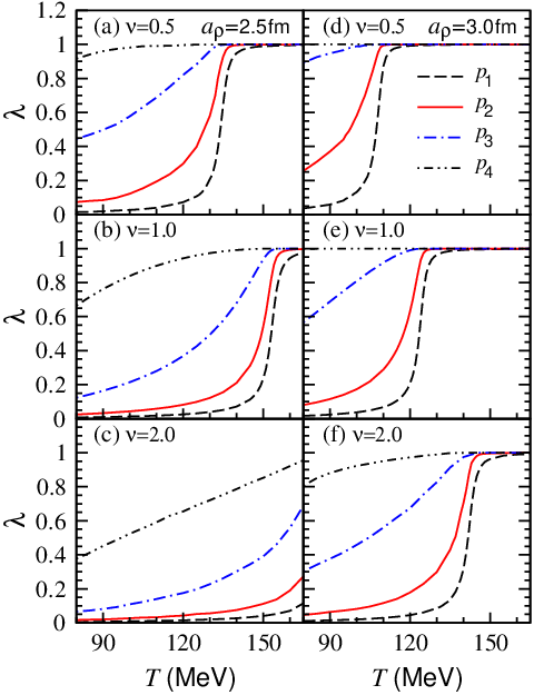
In Fig. 12 we plot the condensed fraction and the RMS of transverse coordinate in the temperature range 80 — 165 MeV and for the systems with 2000, 2.5 and 3.0 fm. It can be seen that decreases from about 1 to zero in this temperature range. Correspondingly, values increase with temperature and have obvious enhancements in the transition region from the condensed phase to uncondensed phase. We observe that the effect of condensation is sensitive to the parameter . For the smaller , the values of are larger and the values of are smaller as compared to the results for the larger . For fixed and , increases and decreases with . In Fig. 13 we plot the values in the temperature range 80 — 165 MeV for the systems with 2000, 2.5 and 3.0 fm. Here the momenta MeV/ (). For the smaller momenta, the values of have rapid increases in the transition region from the condensed phase to uncondensed phase. However, the values of for the larger momenta are higher even at the lower temperatures. It is because that most of the particles with large momenta are from the uncondensed high-energy states. The values of increase with and decrease with because of decreases with and increases with .

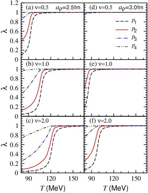
In Figs. 14 and 15 we plot the quantities , , and for the systems with 500 in the temperature range 80 — 165 MeV. Because the critical temperature for 500 is much smaller than that for 2000, the values of are smaller and about zero at most of the temperatures. Correspondingly, the RMS values have obvious increases in only lower temperature regions and increase slowly at most of the temperatures. As compared to the results for the systems with 2000, the values of for 500 are larger. For 3.0 and 0.5, the values of are unity in almost the whole temperature range because the system is completely in the uncondensed phase at almost the whole temperatures.
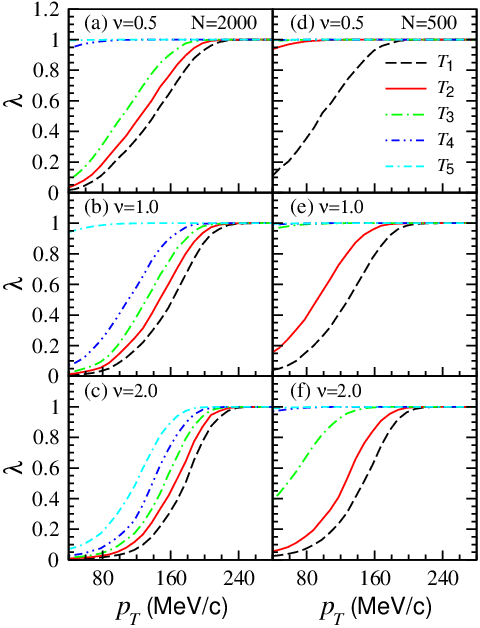
In Fig. 16 we further plot as a function of pion transverse momentum for the systems with fm, 2000 and 500, and 0.5, 1.0, and 2.0, respectively. Here the temperature MeV . It can be seen that the values of increase with and temperature. For fixed and , the values of decrease with increasing particle number and frequency ratio .
In the heavy ion collisions at RHIC, the identical pion multiplicity is about several hundreds. The calculations indicate that in this case the effect of Bose-Einstein condensation on the chaotic parameter in two-pion HBT interferometry may be negligible. However, the identical pion multiplicity in the heavy ion collisions at LHC energy may reach to several thousands. In this case the effect of Bose-Einstein condensation on the two-pion HBT measurements of may be considerable and should be taken into account. From Fig. 12 we observe that the average values of in the transition region are about 6.5 fm for fm and 8.5 fm for fm. The recent two-pion interferometry measurements at LHC indicate that the values of the transverse HBT radius are in the range of 4 — 7 fm [14]. Considering the transverse expansion of the actual particle-emitting source may decrease the transverse HBT radii from the RMS of the source transverse coordinate distribution [3, 15, 16, 17], these average results of are in a reasonable range. Further investigating the effect of Bose-Einstein condensation on the HBT measurements of source radii and chaotic degree in high energy heavy ion collisions, based on a more realistic model of evolving source, will be of great interest.
In our calculations the particle number of system, , is fixed. In this case, the value for an event ensemble with the multiplicity distribution, , is
| (80) |
where is the value for the system with the fixed , as calculated in Sec. IV,
| (81) |
Another calculation of the ensemble value is
| (82) |
Because multiplicity is a observable in high energy heavy ion collisions, and the event number for a certain multiplicity is large and in principle unstinted (by prolonging experimental time), the measurement of the “differential” chaotic parameter is viable and useful in probing the particle source coherence. On the other hand, the appearance of the condensation may modify identical pion multiplicity distribution in high energy heavy ion collisions [6, 7], and thus affect the “integrated” chaotic parameter values and . Investigating the influences of Bose-Einstein condensation on and will be of interest.
V Summary and discussion
We examine the spatial and momentum distributions, two-particle HBT correlation functions, and the chaotic parameter in HBT interferometry for the systems of boson gas within the harmonic oscillator potentials with anisotropic frequencies in transverse and longitudinal directions. The effects of system temperature, particle number, and the average momentum of the particle pair on the chaotic parameter are investigated. Because of Bose-Einstein condensation of boson gas the system is highly condensed at low temperature. This leads to the narrower spatial and momentum distributions of the system, larger width of the HBT correlation functions, and smaller values. When temperature increasing the system becomes uncondensed gradually. The values of increase with temperature and rapidly reach to unity when temperature is closed to and higher than the critical value . For fixed particle number and temperature of system, the values increase with the average momentum of the particle pair because the particles with large momenta are averagely at the uncondensed high-energy states. The results of are sensitive to the ratio, , of the frequencies in longitudinal and transverse directions. They are smaller for larger when is fixed. Because the critical temperature of the system increases with the particle number of system, , the effect of Bose-Einstein condensation on the interferometry measurements of will be significant for a large system. In the heavy ion collisions at LHC energy the identical pion multiplicity may reach to several thousands. In this case the system may possible reach to a considerable condensation. The effect of the condensation on the chaotic parameter in two-pion interferometry is worth considering in earnest. Because we did not consider the particle charge in the model, the results are only suitable for neutral particles, for example . The investigation of the possible change of the results for neutral and charged particles will be of interest.
In experimental HBT analyses, the correlation function is obtained by the ratio of the correlated two particle momentum distribution to the uncorrelated two particle momentum distribution (background) [18, 19]. Here is constructed by the identical particle pairs in which the two particles are from the same event. And is constructed by the two identical particles from the different events with the same global conditions (cuts), such as within a certain region of particle multiplicity (centrality), rapidity, or pseudorapidity, and so on. For the different events, the degree of Bose-Einstein condensation may be different although they have the same global conditions. The difference of the condensation degree for the events may affect the correlated and uncorrelated momentum distributions, and then affect the measurement of the chaotic parameter, corresponding to Eq. (82). However, this influence may become smaller and smaller in principle by imposing stricter and stricter global condition cuts, and it will be an interesting research issue. On the other hand, the model we used in the calculations is only a static system. To make the problem tractable we used the mean-field of harmonic oscillator potential. In fact, the particle-emitting sources produced in high energy heavy ion collisions are expanded and the interactions between the particles in the source are complicated. Further investigating the effect of Bose-Einstein condensation on the HBT measurements of source radii and chaotic degree in high energy heavy ion collisions, based on a more realistic model of evolving source, will be of great interest.
Acknowledgements.
This research was supported by the National Natural Science Foundation of China under Grant Nos. 11075027 and 11275037.References
- [1] M. Gyulassy, K. K. Kauffman, and L. W. Wilson, Phys. Rev. C 20 (1997) 2267.
- [2] Cheuk-Yin Wong, Introduction to High-Energy Heavy-Ion Collisions, World Scientific Publishing Company, Singapore, 1994, Chap. 17.
- [3] U. Wiedemann, U. Heinz, Phys. Rep. 319 (1999) 145.
- [4] R. M. Weiner, Phys. Rept. 327 (2000) 249.
- [5] M. A. Lisa, S. Pratt, R. Soltz, and U. Wiedemann, Ann. Rev. Nucl. Part. Sci. 55 (2005) 357.
- [6] T. Csörgő and J. Zimányi, Phys. Rev. Lett. 80 (1986) 916.
- [7] J. Zimányi and T. Csörgő, Acta Phys. Hung. New Ser. Heavy Ion Phys. 9 (1999) 241.
- [8] Cheuk-Yin Wong and Wei-Ning Zhang, Phys. Rev. C 76 (2007) 034905.
- [9] H. D. Politzer, Phys. Rev. A 54 (1996) 5048.
- [10] M. Naraschewski and R. J. Glauber, Phys. Rev. A 59 (1999) 4595.
- [11] J. Viana Gomes, A. Perrin, M. Schellekens, D. Boiron, C. I. Westbrook, and M. Belsley, Phys. Rev. A 74 (2006) 053607.
- [12] T. Csörgő, R. Vértesi, and J. Sziklai, Phys. Rev. Lett. 105 (2010) 182301.
- [13] R. Vértesi, T. Csörgő, and J. Sziklai, Phys. Rev. C 83 (2011) 054903.
- [14] K. Aamodt et al. (ALICE Collaboration), Phys. Lett. B 696 (2011) 328.
- [15] M. Herrmann and G. F. Bertsch, Phys. Rev. C 51 (1995) 328.
- [16] S. Chapman, P. Scotto, and U. Heinz, Phys. Rev. Lett. 74 (1995) 4400.
- [17] H. J. Yin, J. Yang, and W. N. Zhang, Phys. Rev. C 86 (2012) 024914.
- [18] W. A. Zajc et al. Phys. Rev. C 29 (1984) 2173.
- [19] W. N. Zhang, Y. M. Liu, S. Wang, Q. J. Liu, J. Jiang, D. Keane, Y. Shao, S. Y. Chu, S. Y. Feng, Phys. Rev. C 47 (1993) 795.