Leading-order hadronic contributions to $g_{\mu}-2$

The muon anomalous magnetic moment is among the most precisely measured quantities in physics with $a_{\mu}\equiv\frac{(g_{\mu}-2)}{2}$ determined experimentally to about 0.5 parts per million [1]. Theoretical calculations of Standard Model contributions to $a_{\mu}$ have similar precision. There currently exists tension between Standard Model and experimental determinations of 3.6 standard deviations [2]:

$$a_{\mu}^{\rm exp}-a_{\mu}^{\rm SM}=287(63)(49)\times 10^{-11}.$$

(1)

The possibility that this tension is a hint of beyond Standard Model physics has led to renewed effort to improve the precision of these determinations. The Muon $g-2$ experiment at Fermilab aims to improve the experimental precision to 0.14 parts per million [3].

The full standard model calculation includes contributions from QED, electro-weak and hadronic processes. The uncertainty on the theory side is dominated by the calculation of the hadronic contributions. The current best precision of the leading such contribution, known as the hadronic vacuum polarization (HVP) contribution, comes from experimental $e^{+}e^{-}$ cross-section data [5, 4] and $\tau\rightarrow\nu_{\tau}+$ hadrons decay data [6].

The challenge is for lattice QCD to provide first-principle calculations of the hadronic contributions to $a_{\mu}$ that meet or exceed the current precision of semi-empirical methods. There have been a number of attempts by different lattice groups 5[7, 8, 9, 10, 11] demonstrating the feasibility of the approach. A full calculation will require a calculation of the hadronic vacuum polarization (HVP), including disconnected contributions, as well as the contribution of light-by-light scattering through hadrons.

Here we give a preliminary report of our efforts to calculate the leading-order contribution of the HVP. We present results based on lattices with either 2+1 flavors or four non-degenerate flavors of HEX-smeared clover-type fermions. We include ensembles with pion masses at or below the physical value.

Our preliminary calculations have been performed on the ensembles listed in Table 1. We use HEX-smeared clover-type fermions. We use either two or three levels of HEX smearing. The “2-HEX” ensembles have $N_{f}=2+1$ flavors and are described more fully in [12]. These include ensembles with the pion mass at or below the physical value. The “3-HEX” lattices have four non-degenerate flavors of dynamical fermions, corresponding to $u$, $d$, $s$ and $c$ quarks.

The contribution of the HVP at the lowest order comes from diagrams such as Fig. 1. The lattice method devised by Blum [13] is based on the recognition that these diagrams can be calculated by determining the vacuum-subtracted HVP, $\hat{\Pi}(Q^{2})$ as a function of the square of the Euclidean momentum $Q$, then integrating [14]

$$a_{\mu}^{\rm had,LO}=\frac{\alpha}{\pi}\int^{\infty}_{0}dQ^{2}f(Q^{2})\hat{\Pi}(Q^{2}),$$

(2)

with the kernel function

$$f(Q^{2})=\frac{m^{2}_{\mu}Q^{2}Z(Q^{2})^{3}\left(1-Q^{2}Z(Q^{2})\right)}{1+m_{\mu}^{2}Q^{2}Z(Q^{2})^{2}},$$

(3)

where

$$Z=-\frac{Q^{2}-\sqrt{Q^{4}+4m^{2}_{\mu}Q^{2}}}{2m_{\mu}^{2}Q^{2}}.$$

(4)

On the lattice we calculate for each flavor, $f$, the HVP tensor as the Fourier transform of the vector current correlator:

$$\Pi_{\mu\nu}^{f}(\hat{Q})=a^{4}\sum_{y}e^{iQ(x+\frac{a\hat{\mu}}{2}-y)}\langle J_{\mu}^{\rm CVC}(x)J_{\nu}^{\rm loc}(y)\rangle,$$

(5)

with

$$J^{{\rm loc},f}_{\nu}(y)=\overline{\psi}^{f}(x)\gamma_{\nu}\psi^{f}(x),$$

(6)

and the conserved vector current (CVC) as given by

$$J_{\mu}^{{\rm CVC},f}(x)=\frac{1}{2}\Big[\bar{\psi}^{f}(x+a\hat{\mu})(1+\gamma_{\mu})U_{\mu}^{\dagger}(x)\psi^{f}(x)-\bar{\psi}^{f}(x)(1-\gamma_{\mu})U_{\mu}(x)\psi^{f}(x+a\hat{\mu})\Big].$$

(7)

The HVP tensor satisfies the Ward-Takahashi Identity (WTI) on the conserved index $\mu$:

$$\hat{Q}_{\mu}\hat{\Pi}_{\mu\nu}^{f}=0,$$

(8)

with the modified lattice momentum

$\displaystyle\hat{Q}_{\mu}=\frac{2}{a}\sin\left(\frac{aQ_{\mu}}{2}\right)$

$\displaystyle\,\,\,\,{\rm and}\,\,\,\,$

$\displaystyle Q_{\mu}=\frac{2\pi n_{\mu}}{L_{\mu}}.$

(9)

To enforce conservation on the local current sink index $\nu$ we require $Q_{\nu}=0$. We also use diagonal $\mu=\nu$ elements only.

With Euclidean momentum $Q_{\mu}$, the vacuum-subtracted HVP scalar $\hat{\Pi}(Q^{2})$ appearing in (2) is related to the HVP tensor $\Pi_{\mu\nu}^{f}(Q)$ through

$$\Pi_{\mu\nu}^{f}(Q)=\left(Q^{2}\delta_{\mu\nu}-Q_{\mu}Q_{\nu}\right)\Pi^{f}(Q^{2})$$

(10)

and

$$\hat{\Pi}(Q^{2})=4\pi\alpha\sum_{f=0}^{N_{f}}q_{f}^{2}\left(\Pi^{f}(Q^{2})-\Pi^{f}(0)\right),$$

(11)

where $q_{f}$ is the electromagnetic charge of quark flavor $f$.

To perform the vacuum subtraction in (11) we must know the value of $\Pi^{f}(0)$, which is not directly accessible from the lattice data. To do so we fit the measured values of $\Pi^{f}(0)$ to a suitable function of $Q^{2}$ and extrapolate to $Q^{2}=0$. For simplicity in this preliminary work we fit to:

$$\Pi(Q^{2})=c+\sum_{i=0}^{N}\frac{b_{i}}{Q^{2}+c_{i}},$$

(12)

a multi-vector-dominance model, with $N=1$ or 2, as the data support. Golterman et al.[15] note that this is not an optimal fit ansatz. In the final calculation we will explore different fit forms to constrain systematic errors.

An example of the fits to unsubtracted HVP scalars is shown in Fig. 2. The vector dominance model suggests that the HVP scalar should behave approximately as

$$\Pi^{\rm tree}(Q^{2})=\frac{2}{3}\frac{f^{2}_{V}}{Q^{2}+m^{2}_{V}}.$$

(13)

As a consistency check we compare values of $M_{\rho}$ and $f_{\rho}$ obtained from the fits ($M_{\rho}^{\rm HVP}\equiv c_{0}^{1/2}$ and $f_{\rho}^{\rm HVP}\equiv\sqrt{3b_{0}/2}$) respectively with those extracted from straightforward spectroscopy fits of the zero-momentum correlators. These comparisons are shown in Figs. 3a and 3b.

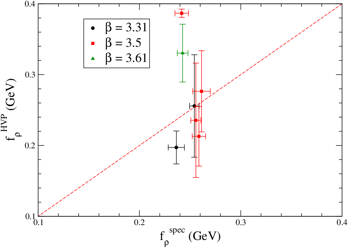
To determine $a_{\mu}^{\rm had,LO}$ we use the fitted parameters to define a continuous function $\Pi(Q^{2})$ with (12), substitute the resulting $\hat{\Pi}(Q^{2})$ into the integral (2), which we evaluate numerically.

In Figs. 6a and 6b we display our preliminary results with statistical error bars only. Fig. 6a shows the value of $a_{\mu}^{\rm had,LO}$ we obtain for the various ensembles, as a function of $M_{\pi}^{2}$. We show results from some other groups for comparison. Figure 6b shows only our physical $M_{\pi}$ ensemble results with other determinations (including calculations with experimental input).

Our future work will refine these calculations, with more ensembles, higher statistics and a full error budget. We also plan to include an estimate of the disconnected contribution.

The authors thank the Gauss Centre for Supercomputing (GCS) for providing computing time through the John von Neumann Institute for Computing (NIC) on the GCS share of the supercomputer JUQUEEN at Jülich Supercomputing Centre (JSC) and time granted on JUROPA at JSC. Computations were also performed using HPC resources provided by GENCI-[IDRIS] (grant 52275). This work was supported in part by the OCEVU Labex (ANR-11-LABX-0060) and the A*MIDEX project (ANR-11-IDEX-0001-02) funded by the “Investissements d’Avenir” French government program managed by the ANR. This work was in part funded by the “Deutsche Forschungsgemeinschaft” under the grant SFB-TR55.

References

- [1] G. W. Bennett et al. [Muon G-2 Collaboration], Phys. Rev. D 73, 072003 (2006) [hep-ex/0602035].
- [2] J. Beringer et al. (Particle Data Group), Phys. Rev. D86, 010001 (2012).
- [3] http://muon-g-2.fnal.gov/.
- [4] K. Hagiwara, et al., JPHGB G38, 085003 (2011).
- [5] M. Davier, et al., Eur. Phys. J. C66, 127 (2010). M. Davier, et al., Eur. Phys. J. C71, 1515 (2011).
- [6] R. Alemany, et al., Eur. Phys. J. C2, 123 (1998).
- [7] C. Aubin and T. Blum, Phys. Rev. D 75, 114502 (2007) [hep-lat/0608011].
- [8] P. Boyle, et al. Phys. Rev. D 85, 074504 (2012) [arXiv:1107.1497].
- [9] X. Feng, et al., Nucl. Phys. Proc. Suppl. 225-227, 269 (2012) [arXiv:1112.4946].
- [10] M. Gockeler et al. [QCDSF Collaboration], Nucl. Phys. B 688, 135 (2004) [hep-lat/0312032].
- [11] M. Della Morte, et al. PoS LATTICE 2012, 175 (2012) [arXiv:1211.1159].
- [12] S. Durr, et al., JHEP 1108, 148 (2011) [arXiv:1011.2711]; Phys. Lett. B 701, 265 (2011) [arXiv:1011.2403].
- [13] T. Blum, Phys. Rev. Lett. 91, 052001 (2003) [hep-lat/0212018].
- [14] B. E. Lautrup, A. Peterman and E. de Rafael, Phys. Rept. 3 (1972) 193; Nuovo Cim. A 1 (1971) 238.
- [15] M. Golterman, K. Maltman and S. Peris, [arXiv:1309.2153].
- [16] C. T. Sachrajda and G. Villadoro, Phys. Lett. B 609, 73 (2005) [hep-lat/0411033].
- [17] C. Aubin, T. Blum, M. Golterman and S. Peris, Phys. Rev. D 88, 074505 (2013) [arXiv:1307.4701].
- [18] K. G. Chetyrkin, J. H. Kuhn and M. Steinhauser, Nucl. Phys. B 482, 213 (1996) [hep-ph/9606230].
- [19] M. Davier, et al., Eur. Phys. J. C 71, 1515 (2011) [arXiv:1010.4180].
- [20] K. Hagiwara, et al., J. Phys. G 38, 085003 (2011) [arXiv:1105.3149].