A little more Gauge Mediation and the light Higgs mass

Gauge mediated supersymmetry breaking [1, 2, 3, 4] (for earlier works, please see, [5, 6, 7, 8, 9, 10, 11]) attractive due to several interesting features (i) flavour blind supersymmetry breaking soft terms (ii) very few parameters determine the entire spectrum (iii) different collider phenomenology compared to gravity mediated models as typically gravitino is the lightest supersymmetric particle (LSP) etc. However, phenomenologically¹¹ 1 For an early phenomenology of these models, please see, [12, 13, 14]. the minimal versions of gauge mediation are severely constrained due to the discovery of a Higgs particle with a mass around 125 GeV. In MSSM, for the lightest CP even Higgs to be around 125 GeV would require, stop mixing parameter $X_{t}$ to be large, $X_{t}\sim\sqrt{6}M_{S}$, where $M_{S}=\sqrt{m_{\tilde{t}_{1}}m_{\tilde{t}_{2}}}$. While this holds true as long as stops are light $\sim 1~\text{TeV}$, for very heavy stops $\gtrsim 4\,\text{TeV}$, the mixing parameter can be smaller. This would however push stops out of the reach of the LHC. In spite of theoretically appealing features, unfortunately, in minimal gauge mediation, the only way to fit a light Higgs mass $\sim 125~\text{GeV}$ is by making stops very heavy. The typical trilinear couplings in these models are very small at the mediation scale $\sim 0$. Renormalisation group (RG) effects do generate them at the weak scale, however their magnitude is not large enough unless one makes gluinos ultra heavy $\sim$ several TeV [15]. It should be noted that the constraints from 125 GeV Higgs boson are stronger even if one moves away from minimal mediation models to general gauge mediation models as long as $A_{t}$ remains zero at the messenger scale [16].

Several possible solutions have been explored in the literature [17, 18, 19, 20, 21, 22, 23, 24, 25, 26, 27, 28, 29, 30, 31, 32, 33, 34]. One of the directions which is popular with many authors is to introduce direct Yukawa couplings between messenger fields and the MSSM fields in addition to gauge interactions [35, 36]. In some cases, these interactions could also violate flavour [37]. In most of the models it is possible to generate large enough $A_{t}$ at the weak scale to fit the 125 GeV light CP even Higgs boson mass. In a recent survey [19, 38] it has been pointed out that a particular class of messenger-matter interactions, messenger- stop mixings, has the least fine tuning of all the possible models which fit the light Higgs mass. Another direction which has been considered is to add additional vector like quarks close to the weak scale which couple to the Higgs superfields. These lead to additional corrections to the light Higgs boson thus lifting its mass without the need of increasing the stop masses (see for example, [31, 30, 32]).

In the following we would like to take an alternate route. We would like to keep the minimal mediation structure in tact, thus would not like to introduce direct couplings between matter and messenger fields. Adding an additional singlet field, like in NMSSM could help to raise the light Higgs mass. There are however, problems with electroweak symmetry breaking while incorporating NMSSM in minimal gauge mediation. These are well documented in literature [39, 40]. There are ways out, either by adding additional matter fields or dynamics through which NMSSM can be made viable with minimal gauge mediation [41, 42, 43, 44, 45, 46, 47, 48, 49, 50]. Post 125 GeV Higgs boson, a model within this class has been explored in [26].

In the present work, we will consider an additional U(1) gauge group under which the ‘singlet’ of the NMSSM is charged. This U(1) factor also participates in gauge mediation. Anomaly cancellation requires additional vector like matter to be present. Such vector like matter is typically introduced to generate correct electroweak symmetry breaking while incorporating NMSSM in minimal mediation models [40]. In the present case, it is motivated from anomaly cancellation requirements. It should be noted that this kind of model has been considered earlier by the authors of Ref. [41]. Ours is a more explicit realisation of it in the sense that we have taken care of $U(1)$ charges and anomaly cancellation conditions. Furthermore, we have performed a more detailed analysis of the Higgs masses in the light of 125 GeV Higgs discovery.

We found that it is possible to find an appropriate set of rational U(1) charges which satisfy the anomaly cancellation conditions as well as allow the correct set of terms in the superpotential. Electroweak symmetry breaking is possible as the U(1) charged singlet can achieve a reasonable vacuum expectation value (vev). Two factors contribute to the raise in the lightest CP even Higgs mass: the effective $\mu$ term is sufficiently large $\sim 0.5-1\,\text{TeV}$ and secondly the RG generated $A_{t}$ term is large compared to minimal gauge mediation. The later is because at the 1-loop level, the $SU(3)$ beta function, $b_{3}$ is zero in this model and the 2-loop $b_{3}$ is not sufficiently large. Together they result in sufficient $X_{t}$ to ensure large mixing in the stop mass matrix. It is possible to find reasonable parameter space which gives correct lightest CP even Higgs mass and satisfy direct constraints from LHC as well as constraints from $Z-Z^{\prime}$ mixing.

The rest of the paper is organised as follows: In the next section particle spectrum and the model are presented. The details of supersymmetric spectrum and various constraints on the parameter space are discussed in section 3. Numerical results are presented in section 4. We close with an outlook in section 5.

The basic premise of the model is that the singlet of the NMSSM should no longer be a singlet, but instead, it is charged under an extension of the Standard Model gauge group such that it receives non-zero supersymmetry breaking contributions at the mediation scale. As it will be detailed in the next section this would help in attaining a large enough vacuum expectation value for the field ‘S’. In this present work, we try to do this by considering the simplest extension in terms of a $U(1)$. The relevant field $S$ is singlet under the Standard Model gauge group, but charged under the extra $U(1)$ ; as a consequence of which all the Standard Model fields are charged under the $U(1)$. The total gauge group is

where the first three represent the usual Standard Model gauge group and the additional gauge group is represented by a subscript A. $U(1)_{A}$ is a chiral gauge group and hence introduces an extra set of anomalies which need to be canceled for a consistent quantum field theory. This imposes a set of conditions on the $U(1)_{A}$ charges; they are listed in Appendix A. We insist that the anomalies cancel independently for the NMSSM sector and the Messenger sector. It is easily verified that the MSSM particle spectrum along with the new field $S$ is not sufficient to cancel all the anomalies. In particular, from $(U(1)_{A}-[SU(3)_{c}]^{2})$ anomaly condition we get

where $A_{1}(exotics)$ is the contribution of the new exotic fields which need to be added and $s$ is the $U(1)_{A}$ charge of the field $S$. The $U(1)_{A}$ charge $s$ cannot be zero as per our requirements. Furthermore, to generate the effective $\mu$ term ($\lambda SH_{u}H_{d}$) in the super-potential, the charge $s$ should be equal to

where $h_{1}$ and $h_{2}$ are the $U(1)_{A}$ charges of $H_{1}$ and $H_{2}$ respectively. We thus need coloured exotics to satisfy $U(1)_{A}-[SU(3)_{c}]^{2}$ anomaly. The number of the exotics is fixed by other anomaly conditions as well as by the $U(1)_{A}$ gauge invariance of the super-potential. It turns out that one possible minimal set of exotic fields would be three families of $SU(2)_{L}$ singlet coloured exotics. We introduce a pair of colour fundamental and anti-fundamentals $D_{i}$ and $\bar{D}_{i}$, which are $SU(2)$ singlets, for each of the three families. In addition to the QCD interactions they are allowed to couple with the field $S$ in the super-potential. The total particle spectrum and their corresponding representations and the $U(1)_{A}$ charges , in the order of Eq. (1) are given in the table below.

where $i$ represents the generation index running from 1 to 3. In the rest of the paper, we will consider all the $U(1)_{A}$ charges to be universal over all the generations and thus suppress the generation index. The only exception to this rule is the $U(1)_{A}$ charges of exotics $z_{i}$. We will consider them to be different for each of the generation, subject to the constraint that in each generation, $z_{i}+\bar{z}_{i}=-s$. The super-potential is given by

where $Y_{E},\,Y_{D},\,Y_{U},\lambda$, $\kappa_{i}$ are Yukawa couplings and we have suppressed generation and colour indices. Note that the field S does not have cubic self interactions.

We will consider a minimal set of messengers communicating the effect of spontaneous supersymmetry breaking in the hidden sector. The spurion $X$ couples to the messengers with the super-potential

where $\Phi$ are messengers in fundamental representation of an $SU(N)\supset G_{SM+A}$ gauge group and $\eta$ is some Yukawa coupling. The resultant soft terms can easily be generalised with the extra $U(1)_{A}$ and can be verified with the wave-function methods of Refs. [51, 52]. The mass terms for the gauginos and soft mass squared terms for the scalars at the mediation scale, $X$ are given as follows²² 2 In writing the formulae Eq.(7) we have suppressed the 1-loop and 2-loop functions. They are however taken in to account in the numerical analysis:

where through an abuse of notation, we have expanded the spurion as $<X>=X+\theta^{2}F_{X}$ and defined $\Lambda={F_{X}/X}$. $C_{i}(f)$ are quadratic Casimirs for the fields $f$ under the four gauge groups. The index $i$ here runs over all the four gauge groups of Eq.(1). We denote the gauge coupling corresponding to $U(1)_{A}$ as $g_{4}$ and we can see, the soft mass of $S$ has the following non-zero value at the $X$ scale :

where we used the standard notation of $\tilde{\alpha}_{i}=\alpha_{i}/(4\pi)$ and $\alpha_{i}=g_{i}^{2}/(4\pi)$. Similarly, we christen $M_{4}$ to be the neutral gaugino corresponding to $U(1)_{A}$ group. It’s mass is given by

The presence of additional $U(1)_{A}$ also introduces additional splittings between the mass squared terms at the mediation scale $X$. For example, the slepton doublets and the Higgs which are degenerate at the high scale in Minimal case, get split as:

However, as we will see later the freedom of these splits is limited as the choice of $U(1)_{A}$ is quite restricted due to phenomenological constraints and anomaly cancellation conditions. Finally, just as in the minimal messenger model, the trilinear $A$ -terms and bilinear $B$ terms remain zero at the mediation scale $X$.

The soft terms at the weak scale can be evaluated by using the relevant Renormalisation Group (RG) equations with the above boundary conditions, Eq.(7). One interesting aspect about the one loop beta functions for the gauge couplings is that the beta function of $SU(3)$, $b_{3}^{(1)}=0$. This is due to the presence of the additional colour triplets $D,\bar{D}$ in three generations³³ 3 We have not explored in the present work about the possibility of making this model finite in the UV (see for example [53]).. As the $\alpha_{s}$ does not run at the 1-loop level, most coloured particles receive larger corrections in RGE running, compared to the Minimal messenger model. This has consequences for the running of $y_{t}$ and subsequently to all the parameters which depend on $y_{t}$ or $A_{t}$. We have used 1-loop RGE for the soft terms and added 2-loop RGE’s for the gauge couplings and Yukawa couplings in this analysis. The relevant RGE for this model are given in Appendix C.

Before proceeding further, a comment about kinetic mixing is in order. The U(1) gauge fields can mix through the kinetic terms of the type $\chi\int d\theta~\mathcal{W}^{A}\mathcal{W}_{Y}$. The current bounds on $\chi$ limit it to $10^{-3}$[54]. We expect that the implications on the phenomenology to be discussed in our paper will be minimally affected due to the presence of the kinetic mixing. For this reason, we will neglect all its effects in the subsequent discussion.

At the weak scale, $M_{SUSY}\sim 1\,\text{TeV}$, we impose electroweak symmetry breaking conditions along with the $U(1)_{A}$ breaking. The neutral Higgs scalar potential is given by

where

The neutral components of the Higgs fields $H_{1}$ and $H_{2}$ get vacuum expectation values (VEV) at the weak scale, $\frac{v_{1}}{\sqrt{2}}$ and $\frac{v_{2}}{\sqrt{2}}$. The field $S$ also gets a VEV, $\frac{v_{s}}{\sqrt{2}}$ at the weak scale, breaking the $U(1)_{A}$ symmetry spontaneously. At the minima of the potential, the vevs and the soft terms along with the other parameters of the model get related. These minimisation conditions are given as

where $G^{2}=g_{1}^{2}+g_{2}^{2}$. The minimisation conditions are modified compared to the standard NMSSM case due to the presence of terms proportional to $g_{4}$. Subsequently, we can see from Eq. (18), that in the limit $v_{s}\gg v_{1},v_{2}$($v_{s}$ is required to be large which is discussed later in this section), we have

which is the typical vev one expects in extra U(1) models [55, 41]. At the high scale, $X$, $m_{S}^{2}$ which is positive and proportional to $\tilde{\alpha}_{4}^{2}\Lambda^{2}$ can be driven negative at the electroweak scale by the Yukawa couplings of the exotics $k_{1},k_{2},k_{3}$ .

This should be contrasted with the vev in minimal gauge mediation, without the $U(1)$ factor. See for example,Refs.[ [39, 56] ]. From the minimization conditions of NMSSM, we get

which is too small to get $\mu_{eff}$ ($\frac{\lambda v_{s}}{\sqrt{2}}$) of the order of electroweak symmetry breaking. To achieve a significant value either $\lambda$ has to be very large ($>1$) or $\kappa$ has to be too small. In both the cases, achieving electroweak symmetry breaking is highly constrained [57]. We now turn our attention to the Higgs sector. The CP-even tree-level Higgs mass squared matrix, $\Psi^{\dagger}\mathcal{M}_{+}^{2}\Psi$, where $\Psi^{T}=\{H_{1}^{0},H_{2}^{0},S\}$, and the elements of the matrix are given as:

Given that the physical Higgs spectrum should be non-tachyonic, we can derive constraints on the parameter space of the model. Firstly the sign of the determinant of the matrix, in the limit $v_{s}>>v_{1,2}$ is crucially dependent on the sign of the $A_{\lambda}$. This is obvious, by considering the full determinant of the $3\times 3$ mass matrix, which is given by

For $A_{\lambda}>0$, the region in which the sign of the determinant of the Higgs mass matrix changes is plotted in $\lambda,g_{4}$ plane by taking $h_{1}=-\frac{1}{2},h_{2}=-\frac{5}{2},s=3$, and $\tan{\beta}=10$. Electroweak symmetry breaking is not possible for the shaded region ($Det<0$) in the parameter space. From the figure, it is seen that for $g_{4}\lesssim 0.1$, large values of $\lambda\gtrsim 0.6$ are disfavoured as they do not allow electroweak symmetry breaking.

The question then arises, whether $A_{\lambda}>0$ ?. Typically the A terms are negative due to the RG running from the high scale. However, in this case, $A_{\lambda}$ turns out to be $\mathcal{O}(10)$ and positive at the weak scale. This positive $A_{\lambda}$ ensures us a safe electroweak vacuum. This is shown in the left panel of Figure 2 , where we have plotted $A_{\lambda}$ with respect to running scale. As we see from the figure 2, $A_{\lambda}$ initially turns negative and then increases turning positive at the weak scale. This happens because of the complicated coupling between $A_{t}$ and $A_{\lambda}$ RGE. The RGE of these parameters are presented in the Appendix C along with the other parameters. In the below, we reproduce them:

Compared to the minimal gauge mediated models, the running effects on the parameter $A_{t}$ are very large as $\alpha_{3}$ barely runs in this models. As mentioned above, $b_{3}=0$ at 1-loop and is very small, at the 2-loop. For this reason, after the SUSY threshold $M_{S}\sim 1\text{TeV}$, $\alpha_{s}$ barely runs all the way to the mediation scale. Due to this $Y_{t}$ and $A_{t}$ receive comparatively large corrections due to the relatively large $\alpha_{s}$. Additional corrections from $g_{4},k_{i}$ and $A_{k_{i}}$ also contribute in the running of the $A_{\lambda}$. This feeds into $A_{\lambda}$, making it positive at the weak scale. In the right panel of the Fig [2], we show the running of the $A_{t}$ for the same parameters

Let us focus our attention to the lightest Higgs mass eigenvalue. The matrix Eq.(20) gives an upper bound on the tree level lightest Higgs mass. In the present model, it has additional contribution from $\lambda$ and $g_{4}$ which is given as

In the NMSSM, it is well known that the tree level contribution can be appreciably enhanced from the MSSM tree level values only for large values of $\lambda\gtrsim 0.7$. The above bound is thus saturated only for special values of the parameters. For most of the parameter space, however the actual eigenvalue is far below the above bound. As in MSSM, one loop corrections would play a major role.

The total number of parameters are $\Lambda$, $M_{X}$, $g_{4}$, $\lambda$ and the $U(1)$ charges. Before proceeding to present the numerical results, we discuss the possible constraints on the various parameters. The first constraint we discuss is from the neutral gauge boson mixing. The neutral gauge bosons $Z$ and $Z^{\prime}$ mix with their mass matrix given by $\mathcal{L}~\supset~\chi^{T}\mathcal{M}_{Z^{\prime}Z}^{2}\chi$ where $\chi^{T}=\{Z^{\prime},Z\}$ with

where

The mixing of the matrix is given by

The current limits on $M_{Z^{\prime}}$ require it to be greater than 1 TeV [58]. For $g_{4}\sim g_{1}$, these limits already push $v_{s}$ to be much larger than 1 TeV. $\Theta_{ZZ^{\prime}}$ is constrained by electroweak precision data, it should be less than $O(10^{-3})$ [54]. As $v_{s}$ is already very heavy with $M_{Z}^{\prime}$ of a mass of TeV order, the constraint on mixing angle is avoided easily.

A second constraint comes from the mass spectrum of the scalar super-partners. The D-terms due to the new $U(1)_{A}$ group play an important role in determining the sfermion mass spectrum due to the large vev of the $S$ field. The strongest effects are felt in the stau mass matrix which is given as:

where

Notice that for the $D_{L}$ and $D_{e}$ to have positive values, the products of the $U(1)_{A}$ charges, $ls$ and $es$ should always be positive. This is because unlike $m_{\widetilde{Q}}^{2},m_{\widetilde{u}}^{2}$ and $m_{\widetilde{u}}^{2}$, the value of $m_{\widetilde{L}}^{2}$ at electroweak scale due to running is very low, as it should be, owing to the fact that $y_{\tau}\ll y_{t}$. So the sign of the diagonal terms in the stau mass squared matrix depends on the $D_{L}$ and $D_{e}$ which in turn depends on the dominant term $l\,s\,g_{4}^{2}\,v_{s}^{2}$. If we choose $U(1)_{A}$ charges $l$ and $s$ of different signs we expect tachyonic masses for stau’s.

The chargino mass matrix remains unaltered compared to the MSSM whereas the neutralino mass matrix is now expanded to include the neutral gauging of $U(1)_{A}$ as well as the fermionic partner of the $S$ field. Note that the fermonic partner of the $S$ is not exactly the singlino as it carries a $U(1)_{A}$ charge unlike the NMSSM case. To summarise the constraints, we have :

• •

  For consistent electroweak breaking : we need, $\lambda$ $=\sqrt{2}\,\,\frac{\mu_{eff}}{v_{s}}$ and $A_{\lambda}>0$. So $\lambda$ cannot be arbitrarily large for a given $g_{4}$ which is evident from the Figure 1

• •

  From $Z-Z^{\prime}$ mixing: we require that $v_{s}\sim$  $O(TeV)\gg v_{1},v_{2}$

• •

  Sfermion masses: From the $D$-terms of the sfermion mass matrices, we require that $U(1)_{A}$ charges $l$ and $s$ should have opposite signs

• •

  Landau pole:the new gauge coupling

  $$g_{4}<2\pi\sqrt{\frac{2}{b_{4}\log\frac{M_{X}}{M_{z}}}}.\\$$

  $g_{4}\approx 0.28$ for $b_{4}=145$ and $M_{X}=100$  TeV

To compute the sparticle spectrum at the weak scale, we use a modified version of the publicly available code SuSeFLAV [59] with 2-loop RGE for the gauge couplings and the Yukawa couplings. The RGE for the rest of the soft parameters are evaluated at the 1-loop level. For the Higgs spectrum, we compute the full 1-loop effective potential corrections presented in Appendix D. These corrections come from stop-top loop and the exotic quarks loop. Stop-top loop correction is the dominant contributor to the Higgs mass at the one loop. The correction due the exotic quarks is significant. It changes Higgs mass by few percent and we have checked that it is possible to get Higgs mass of 125 GeV by adding both the corrections, although we have not considered exotic quarks loop correction to the Higs mass in the numerical analysis. The free parameters are $\Lambda$, $\tan{\beta}$, $\lambda$, $g_{4}$, $k_{1}$, $k_{2}$ and $k_{3}$. These are randomly fixed at the low energy scale, for each set of these parameters, using RGEs we obtain corresponding values at the GMSB scale $X\simeq\Lambda$. Now along with the boundary conditions for the soft masses and A-terms, the same parameters are run down to the electroweak scale to check whether they satisfy minimization conditions given in section (2) and other constraints presented in section (3). This process is repeated several times to obtain a parameter space which satisfy electroweak symmetry breaking conditions. Subsequent to this, we impose phenomenological constraints from direct SUSY searches at LHC [60, 61] as well as the flavour constraints from $b\to s+\gamma$ and $b\to s+\mu^{+}\mu^{-}$.

In the numerical analysis, we fix the $U(1)_{A}$ charges to be as given in Table 1. It should be noted that these are not the only solutions available from anomaly cancellation conditions. A list of five solutions is presented in Appendix A. Of the remaining parameters, we have fixed $\tan\beta=10$ and varied the remaining parameters within a range presented in Table (2).

Instead of presenting the results in terms of regions of allowed parameter space, we present the correlations of the parameters with the lightest CP even Higgs boson mass. In Fig. (3), we present the correlation of the light Higgs mass with respect to the $A_{t}$ generated at the weak scale. The left panel presents the total Higgs mass whereas the right panel shows the 1-loop correction to the light Higgs mass. As expected we see that as $|A_{t}|$ increases, the 1-loop correction to the Higgs mass increases so does the total mass. It is also surprising to see larger values for $A_{t}\sim 900~\,GeV$ possible in this case and accordingly the higher values for Higgs mass $\sim 140~\,GeV$. Of course, the heavier Higgs masses correspond to heavier stops. Note that we have considered only dominant 1-loop corrections to the light Higgs mass. Two loop contributions [62] can be important and they would give a more precise number for the light Higgs mass. However, it is clear that one can easily achieve a light Higgs mass of $\mathcal{O}(125)\,\text{GeV}$.

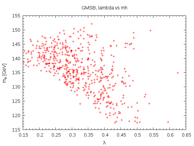
In Fig. (4), we present the correlation between $m_{h}$ and $\lambda$ in the left panel and $m_{h}$ and $g_{4}$ in the right panel. We find a surprising relation between $\lambda$ and $m_{h}$. The Higgs mass seems to be lower for higher values of $\lambda$. This is contrary to expectations based on NMSSM. This is because for higher values of $\lambda$ achieving electroweak symmetry breaking becomes harder. Similarly, larger values of $\lambda$ typically mean lighter values of $v_{s}$. Similarly, larger values of $g_{4}$ are not preferred by the data as they can lead to Landau poles. This can be seen from the right panel of Fig.(4). Thus, the regular NMSSM like enhancement of the tree level Higgs mass is not possible in this model.

From the allowed parameter space, we now present a representative point, Point(A) which give the lightest Higgs mass to be around 125 GeV. In this point, the next to lightest supersymmetry particle (NLSP) is the A-ino, the supersymmetric partner for the extra $U(1)_{A}$ gauge boson.

The discovery of a Higgs boson at 125 GeV has led to strong constraints on the gauge mediated supersymmetry breaking models. Most of the present models have concentrated on generating the required large trilinear $A_{t}$ coupling through messenger matter interactions. In the present work, we tried a different approach of combining the ideas of an extra $U(1)$ factor and NMSSM like models. Anomaly cancellation requirement automatically determines the extra particle spectrum of the model. The coloured particles barely run in this model from the weak scale to the mediation scale due to the small value of the strong beta function. This ‘stagnation’ of $\alpha_{s}$ between $M_{SUSY}$ and $M_{mess}$ and the presence of additional U(1) couplings helps for a larger value of the $A_{t}$ at the $M_{SUSY}$ even though one starts with zero at the mediation scale. Together with a reasonable value for the $\mu_{eft}=\lambda v_{s}$, this generates the required $X_{t}$ at the weak scale for the light stops.

While we have focussed on getting the right Higgs mass, the rest of the spectrum of the model is also quite interesting. There are heavy exotic coloured particles, new neutralinos which are combinations of the Standard Model singlino and the fermion of the $U(1)_{A}$ gauge boson. The lightest neutralino is still the LSP and could be the dark matter candidate. A study of collider signatures and dark matter issues could be interesting and will be pursued in a future work.

Finally, we have not concentrated on the issue of fine tuning in this model. Though we have not explicitly measured it, it is expected that it could be large as long as $M_{X}$ and $\Lambda$ are close as we have chosen. A reasonable separation between the scales can perhaps reduce the fine tuning (see for example, discussion in [63]).

References

• [1] M. Dine and A. E. Nelson, “Dynamical supersymmetry breaking at low-energies,” Phys.Rev., vol. D48, pp. 1277–1287, 1993.
• [2] M. Dine, A. E. Nelson, and Y. Shirman, “Low-energy dynamical supersymmetry breaking simplified,” Phys.Rev., vol. D51, pp. 1362–1370, 1995.
• [3] M. Dine, A. E. Nelson, Y. Nir, and Y. Shirman, “New tools for low-energy dynamical supersymmetry breaking,” Phys.Rev., vol. D53, pp. 2658–2669, 1996.
• [4] G. Giudice and R. Rattazzi, “Theories with gauge mediated supersymmetry breaking,” Phys.Rept., vol. 322, pp. 419–499, 1999.
• [5] M. Dine, W. Fischler, and M. Srednicki, “Supersymmetric Technicolor,” Nucl.Phys., vol. B189, pp. 575–593, 1981.
• [6] M. Dine and W. Fischler, “A Phenomenological Model of Particle Physics Based on Supersymmetry,” Phys.Lett., vol. B110, p. 227, 1982.
• [7] M. Dine and W. Fischler, “A Supersymmetric GUT,” Nucl.Phys., vol. B204, p. 346, 1982.
• [8] S. Dimopoulos and S. Raby, “Geometric Hierarchy,” Nucl.Phys., vol. B219, p. 479, 1983.
• [9] S. Dimopoulos and S. Raby, “Supercolor,” Nucl.Phys., vol. B192, p. 353, 1981.
• [10] C. R. Nappi and B. A. Ovrut, “Supersymmetric Extension of the SU(3) x SU(2) x U(1) Model,” Phys.Lett., vol. B113, p. 175, 1982.
• [11] L. Alvarez-Gaume, M. Claudson, and M. B. Wise, “Low-Energy Supersymmetry,” Nucl.Phys., vol. B207, p. 96, 1982.
• [12] K. Agashe and M. Graesser, “Improving the fine tuning in models of low-energy gauge mediated supersymmetry breaking,” Nucl.Phys., vol. B507, pp. 3–34, 1997.
• [13] J. A. Bagger, K. T. Matchev, D. M. Pierce, and R.-j. Zhang, “Weak scale phenomenology in models with gauge mediated supersymmetry breaking,” Phys.Rev., vol. D55, pp. 3188–3200, 1997.
• [14] H. Baer, M. Brhlik, C.-h. Chen, and X. Tata, “Signals for the minimal gauge mediated supersymmetry breaking model at the Fermilab Tevatron collider,” Phys.Rev., vol. D55, pp. 4463–4474, 1997.
• [15] P. Draper, P. Meade, M. Reece, and D. Shih, “Implications of a 125 GeV Higgs for the MSSM and Low-Scale SUSY Breaking,” Phys.Rev., vol. D85, p. 095007, 2012.
• [16] P. Grajek, A. Mariotti, and D. Redigolo, “Phenomenology of General Gauge Mediation in light of a 125 GeV Higgs,” JHEP, vol. 1307, p. 109, 2013.
• [17] A. Albaid and K. Babu, “Higgs boson of mass 125 GeV in GMSB models with messenger-matter mixing,” Phys.Rev., vol. D88, p. 055007, 2013.
• [18] M. Frank, L. Selbuz, L. Solmaz, and I. Turan, “Higgs Bosons in supersymmetric U(1)’ models with CP Violation,” Phys.Rev., vol. D87, p. 075007, 2013.
• [19] J. A. Evans and D. Shih, “Surveying Extended GMSB Models with mh=125 GeV,” JHEP, vol. 1308, p. 093, 2013.
• [20] N. Craig, S. Knapen, and D. Shih, “General Messenger Higgs Mediation,” JHEP, vol. 1308, p. 118, 2013.
• [21] L. Calibbi, P. Paradisi, and R. Ziegler, “Gauge Mediation beyond Minimal Flavor Violation,” JHEP, vol. 1306, p. 052, 2013.
• [22] P. Byakti and T. S. Ray, “Burgeoning the Higgs mass to 125 GeV through messenger-matter interactions in GMSB models,” JHEP, vol. 1305, p. 055, 2013.
• [23] J. L. Evans, M. Ibe, and T. T. Yanagida, “Relatively Heavy Higgs Boson in More Generic Gauge Mediation,” Phys.Lett., vol. B705, pp. 342–348, 2011.
• [24] J. L. Evans, M. Ibe, S. Shirai, and T. T. Yanagida, “A 125GeV Higgs Boson and Muon g-2 in More Generic Gauge Mediation,” Phys.Rev., vol. D85, p. 095004, 2012.
• [25] N. Craig, S. Knapen, D. Shih, and Y. Zhao, “A Complete Model of Low-Scale Gauge Mediation,” JHEP, vol. 1303, p. 154, 2013.
• [26] T. T. Yanagida, N. Yokozaki, and K. Yonekura, “Higgs Boson Mass in Low Scale Gauge Mediation Models,” JHEP, vol. 1210, p. 017, 2012.
• [27] T. Jelinski, J. Pawelczyk, and K. Turzynski, “On Low-Energy Predictions of Unification Models Inspired by F-theory,” Phys.Lett., vol. B711, pp. 307–312, 2012.
• [28] M. Abdullah, I. Galon, Y. Shadmi, and Y. Shirman, “Flavored Gauge Mediation, A Heavy Higgs, and Supersymmetric Alignment,” JHEP, vol. 1306, p. 057, 2013.
• [29] M. J. Perez, P. Ramond, and J. Zhang, “Mixing supersymmetry and family symmetry breakings,” Phys.Rev., vol. D87, no. 3, p. 035021, 2013.
• [30] M. Endo, K. Hamaguchi, S. Iwamoto, and N. Yokozaki, “Vacuum Stability Bound on Extended GMSB Models,” JHEP, vol. 1206, p. 060, 2012.
• [31] S. P. Martin and J. D. Wells, “Implications of gauge-mediated supersymmetry breaking with vector-like quarks and a  125 GeV Higgs boson,” Phys.Rev., vol. D86, p. 035017, 2012.
• [32] W. Fischler and W. Tangarife, “Vector-like Fields, Messenger Mixing and the Higgs mass in Gauge Mediation,” 2013.
• [33] G. Bhattacharyya, B. Bhattacherjee, T. T. Yanagida, and N. Yokozaki, “A practical GMSB model for explaining the muon (g-2) with gauge coupling unification,” 2013.
• [34] Z. Kang, T. Li, T. Liu, C. Tong, and J. M. Yang, “A Heavy SM-like Higgs and a Light Stop from Yukawa-Deflected Gauge Mediation,” Phys.Rev., vol. D86, p. 095020, 2012.
• [35] Z. Chacko and E. Ponton, “Yukawa deflected gauge mediation,” Phys.Rev., vol. D66, p. 095004, 2002.
• [36] Z. Chacko, E. Katz, and E. Perazzi, “Yukawa deflected gauge mediation in four dimensions,” Phys.Rev., vol. D66, p. 095012, 2002.
• [37] Y. Shadmi and P. Z. Szabo, “Flavored Gauge-Mediation,” JHEP, vol. 1206, p. 124, 2012.
• [38] “David Shih, Talk at SUSY-2013, ICTP, Trieste, http://susy2013.ictp.it/lecturenotes/01_Monday/Shih.pdf,”
• [39] A. de Gouvea, A. Friedland, and H. Murayama, “Next-to-minimal supersymmetric standard model with the gauge mediation of supersymmetry breaking,” Phys.Rev., vol. D57, pp. 5676–5696, 1998.
• [40] M. Dine, Y. Nir, and Y. Shirman, “Variations on minimal gauge mediated supersymmetry breaking,” Phys.Rev., vol. D55, pp. 1501–1508, 1997.
• [41] P. Langacker, N. Polonsky, and J. Wang, “A Low-energy solution to the mu problem in gauge mediation,” Phys.Rev., vol. D60, p. 115005, 1999.
• [42] U. Ellwanger, C.-C. Jean-Louis, and A. Teixeira, “Phenomenology of the General NMSSM with Gauge Mediated Supersymmetry Breaking,” JHEP, vol. 0805, p. 044, 2008.
• [43] T. Liu and C. E. Wagner, “Dynamically Solving the mu/B(mu) Problem in Gauge-mediated Supersymmetry Breaking,” JHEP, vol. 0806, p. 073, 2008.
• [44] K. Hamaguchi, K. Nakayama, and N. Yokozaki, “NMSSM in gauge-mediated SUSY breaking without domain wall problem,” Phys.Lett., vol. B708, pp. 100–106, 2012.
• [45] K. Hamaguchi, K. Nakayama, and N. Yokozaki, “A Solution to the mu/Bmu Problem in Gauge Mediation with Hidden Gauge Symmetry,” JHEP, vol. 1208, p. 006, 2012.
• [46] S. Dimopoulos, G. Dvali, and R. Rattazzi, “A Simple complete model of gauge mediated SUSY breaking and dynamical relaxation mechanism for solving the mu problem,” Phys.Lett., vol. B413, pp. 336–341, 1997.
• [47] D. E. Morrissey and A. Pierce, “Modified Higgs Boson Phenomenology from Gauge or Gaugino Mediation in the NMSSM,” Phys.Rev., vol. D78, p. 075029, 2008.
• [48] T. Yanagida, “A Solution to the mu problem in gauge mediated supersymmetry breaking models,” Phys.Lett., vol. B400, pp. 109–111, 1997.
• [49] J. de Blas and A. Delgado, “Singlet deflected anomaly/gauge mediation,” Phys.Lett., vol. B708, pp. 300–306, 2012.
• [50] J. de Blas and A. Delgado, “Exploring singlet deflection of gauge mediation,” Phys.Rev., vol. D83, p. 115011, 2011.
• [51] G. Giudice and R. Rattazzi, “Extracting supersymmetry breaking effects from wave function renormalization,” Nucl.Phys., vol. B511, pp. 25–44, 1998.
• [52] N. Arkani-Hamed, G. F. Giudice, M. A. Luty, and R. Rattazzi, “Supersymmetry breaking loops from analytic continuation into superspace,” Phys.Rev., vol. D58, p. 115005, 1998.
• [53] K. Babu, T. Kobayashi, and J. Kubo, “Finite theories and the SUSY flavor problem,” Phys.Rev., vol. D67, p. 075018, 2003.
• [54] A. Hook, E. Izaguirre, and J. G. Wacker, “Model Independent Bounds on Kinetic Mixing,” Adv.High Energy Phys., vol. 2011, p. 859762, 2011.
• [55] V. Barger, P. Fileviez Perez, and S. Spinner, “Minimal gauged U(1)(B-L) model with spontaneous R-parity violation,” Phys.Rev.Lett., vol. 102, p. 181802, 2009.
• [56] U. Ellwanger, C. Hugonie, and A. M. Teixeira, “The Next-to-Minimal Supersymmetric Standard Model,” Phys.Rept., vol. 496, pp. 1–77, 2010.
• [57] A. Delgado, G. Giudice, and P. Slavich, “Dynamical mu term in gauge mediation,” Phys.Lett., vol. B653, pp. 424–433, 2007.
• [58] S. Chatrchyan et al., “Search for anomalous t t-bar production in the highly-boosted all-hadronic final state,” JHEP, vol. 1209, p. 029, 2012.
• [59] D. Chowdhury, R. Garani, and S. K. Vempati, “SUSEFLAV: Program for supersymmetric mass spectra with seesaw mechanism and rare lepton flavor violating decays,” Comput.Phys.Commun., vol. 184, pp. 899–918, 2013.
• [60] ATLAS Collaboration, “https://twiki.cern.ch/twiki/bin/view/AtlasPublic/SupersymmetryPublicResults,”
• [61] CMS Collaboration, “https://twiki.cern.ch/twiki/bin/view/CMSPublic/PhysicsResultsSUS#CMS_Supersymmetry_Physics_Result,”
• [62] S. P. Martin and M. T. Vaughn, “Two loop renormalization group equations for soft supersymmetry breaking couplings,” Phys.Rev., vol. D50, p. 2282, 1994.
• [63] Z. Komargodski and N. Seiberg, “mu and General Gauge Mediation,” JHEP, vol. 0903, p. 072, 2009.
• [64] H.-S. Lee, K. T. Matchev, and T. T. Wang, “A U(1) -prime solution to the μ−\mu^{-} problem and the proton decay problem in supersymmetry without R-parity,” Phys.Rev., vol. D77, p. 015016, 2008.
• [65] S. R. Coleman and E. J. Weinberg, “Radiative Corrections as the Origin of Spontaneous Symmetry Breaking,” Phys.Rev., vol. D7, pp. 1888–1910, 1973.
• [66] N. K. Falck, “Renormalization Group Equations for Softly Broken Supersymmetry: The Most General Case,” Z.Phys., vol. C30, p. 247, 1986.