High-efficiency degenerate four wave-mixing in triply resonant nanobeam cavities
Abstract
We demonstrate high-efficiency, degenerate four-wave mixing in triply resonant Kerr () photonic crystal (PhC) nanobeam cavities. Using a combination of temporal coupled mode theory and nonlinear finite-difference time-domain (FDTD) simulations, we study the nonlinear dynamics of resonant four-wave mixing processes and demonstrate the possibility of observing high-efficiency limit cycles and steady-state conversion corresponding to depletion of the pump light at low powers, even including effects due to losses, self- and cross-phase modulation, and imperfect frequency matching. Assuming operation in the telecom range, we predict close to perfect quantum efficiencies at reasonably low input powers in silicon micrometer-scale cavities.
pacs
Valid PACS appear hereI Introduction
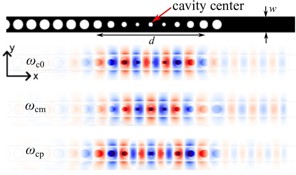
Optical nonlinearities play an important role in numerous photonic applications, including frequency conversion and modulation [1, 2, 3, 4, 5, 6, 7], light amplification and lasing [1, 8, 9, 10], beam focusing [1, 11], phase conjugation [1, 12], signal processing [13, 14], and optical isolation [15, 16]. Recent developments in nanofabrication are enabling fabrication of nanophotonic structures, e.g. waveguides and cavities, that confine light over long times and small volumes [17, 18, 19, 20, 21], minimizing the power requirements of nonlinear devices [22, 23] and paving the way for novel on-chip applications based on all-optical nonlinear effects [18, 24, 25, 26, 27, 28, 29, 30, 31, 32, 33]. In addition to greatly enhancing light–matter interactions, the use of cavities can also lead to qualitatively rich dynamical phenomena, including multistability and limit cycles [34, 35, 36, 37, 38, 39, 40]. In this paper, we explore realistic microcavity designs that enable highly efficient degenerate four-wave mixing (DFWM) beyond the undepleted pump regime. In particular, we extend the results of our previous work [41], which focused on the theoretical description of DFWM in triply resonant systems via the temporal coupled-mode theory (TCMT) framework, to account for various realistic and important effects, including linear losses, self- and cross-phase modulation, and frequency mismatch. Specifically, we consider the nonlinear process depicted in Fig. 1, in which incident light at two nearby frequencies, a pump and signal photon, is up-converted into output light at another nearby frequency, an idler photon, inside a triply resonant photonic crystal nanobeam cavity (depicted schematically in Fig. 8). We demonstrate that 100% conversion efficiency (complete depletion of the pump power) can be achieved at a critical power and that detrimental effects associated with self- and cross-phase modulation can be overcome by appropriate tuning of the cavity resonances. Surprisingly, we find that critical solutions associated with maximal frequency conversion are ultra-sensitive to frequency mismatch (deviations from perfect frequency matching resulting from fabrication imperfections), but that there exist other robust, dynamical states (e.g. “depleted” states and limit cycles) that, when properly excited, can result in high conversion efficiencies at reasonable pump powers. We demonstrate realistic designs based on PhC nanobeam cavities that yield 100% conversion efficiencies at pump powers and over broad bandwidths (modal lifetimes s). Although our cavity designs and power requirements are obtained using the TCMT framework, we validate these predictions by checking them against rigorous, nonlinear FDTD simulations.
Although chip-scale nonlinear frequency conversion has been a topic of interest for decades [33], most theoretical and experimental works have been primarily focused on large-etalon and singly resonant systems exhibiting either large footprints and small bandwidths [25, 26, 42, 43], or low conversion efficiencies (the undepleted pump regime) [22, 44, 45, 46]. These include studies of processes such as second harmonic generation [47, 48, 26, 49], sum and difference frequency generation [50], and optical parametric amplification [28, 27, 51], as well as processes such as third harmonic generation [52, 47], four-wave mixing [53, 54, 55] and optical parametric oscillators [22, 56, 57, 58]. Studies that go beyond the undepleted regime and/or employ resonant cavities reveal complex nonlinear dynamics in addition to high efficiency conversion [38, 23, 37, 39, 59, 41, 60], but have primarily focused on ring resonator geometries due to their simplicity and high degree of tunability [60]. Significant efforts are underway to explore similar functionality in wavelength-scale photonic components (e.g. photonic crystal cavities) [50, 49], although high-efficiency conversion has yet to be experimentally demonstrated. Photonic crystal nanobeam cavities not only offer a high degree of tunability, but also mitigates the well-known volume and bandwidth tradeoffs associated with ring resonators [61], yielding minimal device footprint and on-chip integrability [62, 63], in addition to high quality factors [64, 65, 21, 66, 67].
In what follows, we investigate the conditions and design criteria needed to achieve high efficiency DFWM in realistic nanobeam cavities. Our paper is divided into two primary sections. In Sec. II, we revisit the TCMT framework introduced in [41], and extend it to include new effects arising from cavity losses (Sec. II.1), self- and cross-phase modulation (Sec. II.2), and frequency mismatch (Sec. II.3). In Sec. III, we consider specific designs, starting with a simple 2d design (Sec. III.2) and concluding with a more realistic 3d design suitable for experimental realization (Sec. III.3). The predictions of our TCMT are checked and validated in the 2d case against exact nonlinear FDTD simulations.
II Temporal coupled-mode theory

In order to obtain accurate predictions for realistic designs, we extend the TCMT predictions of [41] to include important effects associated with the presence of losses, self- and cross-phase modulation, and imperfect frequency-matching. We consider the DFWM process depicted in Fig. 1, in which incident light from some input/output channel (e.g. a waveguide) at frequencies and is converted to output light at a different frequency inside a triply-resonant cavity. The fundamental assumption of TCMT (accurate for weak nonlinearities) is that any such system, regardless of geometry, can be accurately described by a few set of geometry-specific parameters [41]. These include, the frequencies and corresponding lifetimes (or quality factors ) of the cavity modes, as well as nonlinear coupling coefficients, and , determined by overlap integrals between the cavity modes (and often derived from perturbation theory [23]). Note that in general, the total decay rate () of the modes consist of decay into the input/output channel (), as well as external (e.g. absorption or radiation) losses with decay rate , so that . Letting denote the time-dependent complex amplitude of the th cavity mode (normalized so that is the electromagnetic energy stored in this mode), and letting denote the time-dependent amplitude of the incident (+) and outgoing () light (normalized so that is the power at the incident/output frequency ), it follows that the field amplitudes are determined by the following set of coupled ordinary differential equations [23]:
| (1) | ||||
| (2) | ||||
| (3) | ||||
| (4) |
where the nonlinear coupling coefficients [41],
| (5) | ||||
| (6) |
| (7) |
| (8) |
| (9) |
express the strength of the nonlinearity for a given mode, with the terms describing SPM and XPM effects and the terms characterizing energy transfer between the modes. (Technically speaking, this qualitative distinction between and is only true in the limit of small losses [23]).
II.1 Losses
Eqs. 1–4 can be solved to study the steady-state conversion efficiency of the system [] in response to incident light at the resonant cavity frequencies (), as was done in [41] in the ideal case of perfect frequency-matching (), no losses (), and no self- or cross-phase modulation (). In this ideal case, one can obtain analytical expressions for the maximum efficiency and critical powers, and , at which 100% depletion of the total input power is attained [41]. Performing a similar calculation, but this time including the possibility of losses, we find:
| (10) | ||||
| (11) |
With respect to the lossless case, the presence of losses merely decreases the maximum achievable efficiency by a factor of while increasing the critical power by a factor of . As in the case of no losses, 100% depletion is only possible in the limit as , from which it follows that the maximum efficiency is independent of . As noted in [41], the existence of a limiting efficiency (Eq. 11) can also be predicted from the Manley–Rowe relations governing energy transfer in nonlinear systems [68] as can the limiting condition . While theoretically this suggests that one should always employ as small a as possible, as we show below, practical considerations make it desirable to work at a small but finite (non-negligible) .
II.2 Self- and cross-phase modulation
Unlike losses, the presence of self- and cross-phase modulation dramatically alters the frequency-conversion process. Specifically, a finite leads to a power-dependent shift in the effective cavity frequencies that spoils both the frequency-matching condition as well as the coupling of the incident light to the corresponding cavity modes. One approach to overcome this difficulty is to choose/design the linear cavity frequencies to have frequency slightly detuned from the incident frequencies , such that at the critical powers, the effective cavity frequencies align with the incident frequencies and satisfy the frequency matching condition [41]. Specifically, assuming incident light at and , it follows by inspection of Eqs. 1–4 that preshifting the linear cavity resonances away from the incident frequencies according to the transformation,
| (12) | ||||
| (13) | ||||
| (14) |
yields the same steady-state critical solution obtained for , where denote the critical, steady-state cavity fields.
An alternative approach to excite the critical solution above in the presence of self- and cross-phase modulation is to detune the incident frequencies away from and , keeping the two cavity frequencies unchanged, while pre-shifting to enforce frequency matching. Specifically, by inspection of Eqs. 12–14, it follows that choosing input-light frequencies
| (15) | ||||
| (16) |
and tuning such that
| (17) |
yields the same steady-state critical solution above. This approach is advantageous in that the requirement that all three cavity frequencies be simultaneously and independently tuned (post-fabrication) is removed in favor of tuning a single cavity mode. Given a scheme to tune the frequencies of the cavity modes that achieves perfect frequency matching at the critical power, what remains is to analyze the stability and excitability of the new critical solution, which can be performed using a staightforward linear stability analysis of the coupled mode equations [38]. Before addressing these questions, however, is important to address a more serious concern.
II.3 Frequency mismatch
Regardless of tuning mechanism, in practice one can never fully satisfy perfect frequency matching (even when self- and cross-phase modulation can be neglected) due to fabrication imperfections. In general, one would expect the finite bandwidth to mean that there is some tolerance on any frequency mismatch [60]. However, here we find that instabilities and strong modifications of the cavity lineshapes arising from the particular nature of this nonlinear process lead to extreme, sub-bandwidth sensitivity to frequency deviations that must be carefully examined if one is to achieve high-efficiency operation.

To illustrate the effects of frequency mismatch, we first consider an ideal, lossless system with zero self- and cross-phase modulation () and with incident light at frequencies and , and powers and , respectively. With the exception of , the coupling coefficients and cavity parameters correspond to those of the 2d design described in Sec. III.2. Figure 2 (top) shows the steady-state conversion efficiency (solid lines) as a function of the frequency mismatch away from perfect frequency-matching, for multiple values of , with blue/red solid lines denoting stable/unstable steady-state fixed points. As shown, solutions come in pairs of stable/unstable fixed points, with the stable solution approaching the maximum-efficiency critical solution as . Moreover, one observes that as increases for finite , the stable and unstable fixed points approach and annihilate one other, with limit cycles appearing in their stead (an example of what is known as a “saddle-node homoclinic bifurcation” [69]). The mismatch at which this bifurcation occurs is proportional to , so that, as , the regime over which there exist high-efficiency steady states reduces to a single fixed point occurring at . Beyond this bifurcation point, the system enters a limit-cycle regime (shaded regions) characterized by periodic modulations of the output signal in time [70, 38, 37]. Interestingly, we find that the average efficiency of the limit cycles (dashed lines),
| (18) |
remains large and even as is several fractional bandwidths. The inset of Fig. 2 (top) shows the efficiency of this system as a function of time (in units of the lifetime ) for large mismatch . As expected, the modulation amplitude and period of the limit cycles depend on the input power and mismatch, and in particular we find that the amplitude goes to zero and the period diverges as . This behavior is observed across a wide range of , with larger leading to lower and larger amplitudes. For small enough mismatch, the modulation frequency enters the THz regime, in which case standard rectifications procedures [71] can be applied to extract the useful THz oscillations [72, 4, 73, 5, 74, 75].
Frequency mismatch leads to similar effects for finite , including homoclinic bifurcations and corresponding high-efficiency limit cycles that persist even for exceedingly large frequency mismatch. One important difference, however, is that the redshift associated with self- and cross-phase modulation creates a strongly asymmetrical lineshape that prevents high-efficiency operation for . Figure 2 (bottom) shows the stable/unstable fixed points (solid lines) and limit cycles (dashed regions) as a function of for the same system of Fig. 2 (top) but with finite , for multiple values of . As before, the coupling coefficients and cavity parameters correspond to those of the 2d design described in Sec. III.2. Here, in contrast to the case, the critical incident frequencies and are chosen according to Eqs. 15–16 in order to counter the effects of self- and cross-phase modulation, and are therefore generally different from and . Aside from the asymmetrical lineshape, one important difference from the case is the presence of additional stable/unstable low-efficiency solutions. Multistability complicates matters since, depending on the initial conditions, the system can fall into different stable solutions and in particular, simply turning on the source at the critical input power may result in an undesirable low-efficiency solution. One well-known technique that allows such a system to lock into the desired high-efficiency solutions is to superimpose a gradual exponential turn-on of the pump with a Gaussian pulse of larger amplitude [37]. We found that a single Gaussian pulse with a peak power of and a temporal width , depicted in the right inset of Fig. 2 (bottom), is sufficient to excite high-efficiency limit cycles in the regime .

Despite their high efficiencies (even for large ), the limit-cycle solutions above leave something to be desired. Depending on the application, it may be desirable to operate at high-efficiency fixed points. One way to achieve this for non-zero frequency mismatch is to abandon the critical solution and instead choose incidence parameters that exploit self- and cross-phase modulation in order to enforce perfect frequency matching and 100% depletion of the pump as follows,
| (19) | ||||
| (20) |
Specifically, enforcing Eqs. 19–20 by solving Eqs. 1–4 for , and , we obtain a depleted steady-state solution that, in contrast to the critical solution , yields a steady-state efficiency that corresponds to 100% depletion of the pump regardless of frequency mismatch. Note that we are not explicitly maximizing the conversion efficiency but rather enforcing complete conversion of pump energy in the presence of frequency mismatch, at the expense of a non-negligible input . Figure 3 shows the depleted steady-state efficiency (solid line) and corresponding incident powers (solid circles and dashed line) as a function of , for the same system of Fig. 2 (bottom). We find that for most parameters of interest, depleted efficiencies and powers are uniquely determined by Eqs. 19–20. As expected, the optimal efficiency occurs at and corresponds to the critical solution, so that , , and . For finite , the optimal efficiencies are lower due to the finite , but there exist a broad range of over which one obtains relatively high efficiencies . Power requirements and follow different trends depending on the sign of . Away from zero detuning, can only increase whereas decreases for and increases for . In the latter case, the total input power exceeds leading to the observed instability of the fixed-point solutions.
Finally, we point out that limit cycles and depleted steady states reside in roughly complementary regimes. Although no stable high-efficiency fixed points can be found in the regime, it is nevertheless possible to excite high-efficiency limit cycles. Conversely, although no such limit cycles exist for , it is possible in that case to excite high-efficiency depleted steady states.
III Nanobeam designs
In this section, we consider concrete and realistic cavity designs in 2d and 3d, and check the predictions of our TCMT by performing exact nonlinear FDTD simulations in 2d. Our designs are based on a particular class of PhC nanobeam structures, depicted schematically in Figs. 4 and 8, where a cavity is formed by the introduction of a defect in a lattice of air holes in dielectric, and coupled to an adjacent waveguide formed by the removal of holes on one side of the defect. We restrict our analysis to dielectric materials with high nonlinearities at near- and mid-infrared wavelengths [1], and in particular focus on undoped silicon, whose refractive index and Kerr susceptibility [76].
III.1 General design considerations
Before delving into the details of any particular design, we first describe the basic considerations required to achieve the desired high efficiency characteristics. To begin with, we require three modes satisfying the frequency-matching condition to within some desired bandwidth (determined by the smallest of the mode bandwidths). We begin with the linear cavity design, in which case we seek modes that approximately satisfy . The final cavity design, incorporating self- and cross-phase modulation, is then obtained by additional tuning of the mode frequencies as described above. Second, we seek modes that have large nonlinear overlap , determined by Eq. 8. (Ideally, one would also optimize the cavity design to reduce , but such an approach falls beyond the scope of this work.) Note that the overlap integral replaces the standard “quasiphase matching” requirement in favor of constraints imposed by the symmetries of the cavity [1]. In our case, the presence of reflection symmetries means that the modes can be classified as either even or odd and also as “TE-like” () or “TM-like” () [77], and hence only certain combinations of modes will yield non-zero overlap. It follows from Eq. 8 that any combination of even/odd modes will yield non-zero overlap so long as and have the same parity, and as long as all three modes have similar polarizations: modes with different polarization will cause the term in Eq. 8 to vanish. Third, in order to minimize radiation losses, we seek modes whose radiation lifetimes are much greater than their total lifetimes, as determined by any desired operational bandwidth. In what follows, we assume operational bandwidths with . Finally, we require that our system support a single input/output port for light to couple in/out of the cavity, with coupling lifetimes in order to have negligible radiation losses.
III.2 2d design
In what follows, we consider two different 2d cavities with different mode frequencies but similar lifetimes and coupling coefficients. (Note that by 2d we mean that electromagnetic fields are taken to be uniform in the direction.) The two cavities follow the same backbone design shown in Fig. 4 which supports three TE-polarized modes () with radiative lifetimes and , and total lifetimes and , respectively. The nonlinear coupling coefficients are calculated from the linear modal profiles (shown on the inset of Fig. 4) via Eqs. 8–7, and are given by:
where the additional factor of allows comparison to the realistic 3d structure below and accounts for finite nanobeam thickness (again, assuming uniform fields in the direction). Compared to the optimal , corresponding to modes with uniform fields inside and zero fields outside the cavity, we find that is significantly smaller due to the fact that these TE modes are largely concentrated in air. In the 3d design section below, we choose modes with peaks in the dielectric regions, which leads to much larger .

In order to arrive at this 2d design, we explored a wide range of defect parameters, with the defect formed by modifying the radii of a finite set of holes in an otherwise periodic lattice of air holes of period and radius in a dielectric nanobeam of width and index of refraction . The defect was parametrized via an exponential adiabatic taper of the air-hole radii , in accordance with the formula , where the parameter is an “effective cavity length”. Such an adiabatic taper is chosen to reduce radiation/scattering losses at the interfaces of the cavity [78]. The removal of holes on one side of the defect creates a waveguide, with corresponding cavity–waveguide coupling lifetimes determined by the number of holes removed [79, 80, 81]. To illustrate the dependence of the mode properties on the cavity parameters, Fig. 5(top) shows the evolution of the cavity-mode frequencies as a function of , with blue/red dots denoting even/odd modes and with larger dots denoting longer modal lifetimes. As expected, the volumes of the modes decrease with decreasing , leading to larger (smaller critical powers) but causing the frequency gap between the modes and radiation losses to increase. We find that the desired modal parameters for FWM lie at some intermediate . In order to tune the relative frequencies between the modes, an additional tuning parameter is required. Specifically, it follows from perturbation theory [61] that changing the central hole radius allows control of the even-mode frequencies while leaving odd-mode frequencies unchanged. Figure 5(bottom) shows the evolution of the cavity-mode frequencies as a function of , for a fixed . As described below, the particular choice of will depend on whether one seeks to operate with high-efficiency limit cycles versus high-efficiency steady-state solutions.
III.2.1 Limit cycles


In this section, we consider a design supporting high-efficiency limit cycles. Choosing , we obtain critical parameters , , , and , corresponding to frequency mismatch and critical efficiency . Choosing a small but finite , it follows from Fig. 2 (dashed line) that the system will support limit cycles with average efficiencies . To excite these solutions, we employed the priming technique described in Sec. II.3. Figure 6 shows as a function of , for incident frequencies determined by Eqs. 15–16, as computed by our TCMT (gray line) and by exact, nonlinear FDTD simulations (solid circles). The two show excellent agreement. For , we observe limit cycles with relatively high , in accordance with the TCMT predictions, whereas outside of this regime, we find that the system invariably falls into low-efficiency fixed points. The periodic modulation of the limit cycles means that instead of a single peak, the spectrum of the output signal consists of a set of equally spaced peaks surrounding . The top and bottom insets of Fig. 6 show the corresponding frequency spectra of the TCMT and FDTD output signals around , for a particular choice of (red circle), showing agreement both in the relative magnitude and spacing of the peaks.
III.2.2 Depleted steady states
In this section, we consider a design supporting high-efficiency, depleted steady states. Choosing , one obtains critical parameters , , , and , corresponding to frequency mismatch and critical efficiency . Choosing incident frequencies , , and incident powers and , it follows from Fig. 3 (dashed line) that the system supports stable, depleted steady states with efficiencies . Figure 7 shows the efficiency of the system as a function , with all other incident parameters fixed to the depleted-solution values above, where blue/red lines denote stable/unstable solutions. As before, we employ the priming technique of Sec. II.3 in order to excite the desired high efficiency solutions and obtain excellent agreement between our TCMT (gray line) and FDTD simulations (solid circles). Exciting the high-efficiency solutions by steady-state input “primed” with a Gaussian pulse is convenient in FDTD because it leads to relatively short simulations, but is problematic for , where the system becomes very sensitive to the priming parameters, and it became impractical in for us to find the optimal FDTD source conditions in Fig. 7. In realistic experimental situations, however, one can use a different technique to excite the high-efficiency solution in a way that is very robust to errors, based on adiabatic tuning of the pump power [37].
III.3 3d design

We now consider a 3d design, depicted in Fig. 8, as a feasible candidate for experimental realization. The cavity supports three TE00 modes () of frequencies and , radiative lifetimes . As before, the total lifetimes can be adjusted by removing air holes to the right or left of the defect, which would allow coupling to the resulting in-plane waveguides. (Alternatively, one might consider an out-of-plane coupling mechanism in which a fiber carrying incident light at both and/or is brought in close proximity to the cavity [79, 82].) In what follows, we do not consider any one particular coupling channel and focus instead on the isolated cavity design. Nonlinear coupling coefficients are calculated from the linear modal profiles (shown on the inset of Fig. 8) via Eqs. 9–7, and are given by:
Here, in contrast to the 2d design of Sec. III.2, we chose modes whose amplitudes are concentrated in dielectric regions, and therefore find appreciably larger.
In order to arrive at the above 3d design, we explored a cavity parametrization similar to the one described in [83]. Specifically, we employed a suspended nanobeam of width , thickness , and refractive index . The beam is schematically divided into a set of lattice segments, each having length and corresponding air-hole radii , where () is the length of the lattice segment immediately to the right (left) of the beam’s center. The cavity defect is induced via a linear taper of over a chosen set of segments, according to the formula:
In order to arrive at our particular design, we chose and varied the central cavity length to obtain the desired TE00 modes. Assuming total modal lifetimes , and and using these design parameters, we obtain critical parameters , , , and , corresponding to frequency mismatch and . Note that because the radiative losses in this system are non-negligible, the maximum efficiency of this system is of the optimal achievable efficiency . At these small , we find that depletion of the pump is readily achieved through the critical parameters associated with perfect frequency matching. However, as illustrated in Sec. III.2.1, it is indeed possible to choose a design that leads to highly efficient limit cycles or other dynamical behaviors.
We now express the power requirements of this particular design using real units instead of the dimensionless units of we have employed thus far. Choosing to operate at telecom wavelengths m, with corresponding and [1], we find that nm and . Although our analysis above incorporates effects arising from linear losses (e.g. due to material absorption or radiation), it neglects important and detrimental sources of nonlinear losses in the telecom range, including two-photon and free carrier absorption [84, 85]. Techniques that mitigate the latter exist, e.g. reverse biasing [86], but in their absence it may be safer to operate in the spectral region below the half-bandgap of silicon [76]. One possibility is to operate at m, in which case [76], leading to nm and . For a more detailed analysis of nonlinear absorption in triply resonant systems, the reader is referred to [87]. While that work does not consider the effects of nonlinear dispersion, self- and cross-phase modulation, or frequency mismatch, it does provide upper bounds on the maximum efficiency in the presence of two-photon and free-carrier absorption.
IV Concluding remarks
In conclusion, using a combination of TCMT and FDTD simulations, we have demonstrated the possibility of achieving highly efficient DFWM at low input powers () and large bandwidths () in a realistic and chip-scale (m) nanophotonic platform consisting of a triply resonant silicon nanobeam cavity. Our theoretical analysis includes detrimental effects stemming from linear losses, self- and cross-phase modulation, and mismatch of the cavity mode frequencies (e.g. arising from fabrication imperfections), and is checked against the predictions of a full nonlinear Maxwell FDTD simulation. Although power requirements in the tens of ms are not often encountered in conventional chip-scale silicon nanophotonics, they are comparable if not smaller than those employed in conventional centimeter-scale DFWM schemes [88, 86, 89]. Our proof-of-concept design demonstrates that full cavity-based DFWM not only reduces device dimensions down to m scales, but also allows depletion of the pump with efficiencies close to unity. However, we emphasize that there is considerable room for additional design optimization. In particular, we find that increasing the radiative lifetimes of the signal and converted modes (currently almost two orders of magnitudes lower than the pump) can significantly lower the power requirements of the system.
Acknowledgements: We acknowledge support from the MIT Undergraduate Research Opportunities Program and the U.S. Army Research Office through the Institute for Soldier Nanotechnology under contract W911NF-13-D-0001.
References
- [1] R. W. Boyd, Nonlinear Optics (Academic Press, California, 1992).
- [2] J. Hald, Optics Communications 197, 169 (2001).
- [3] R. Lifshitz, A. Arie, and A. Bahabad, Phys. Rev. Lett. 95, 133901 (2005).
- [4] Y. A. Morozov, I. S. Nefedov, V. Y. Aleshkin, and I. V. Krasnikova, Semiconductors 39, 113 (2005).
- [5] K.-L. Yeh, M. C. Hoffmann, J. Hebling, and K. A. Nelson, Applied Physics Letters 90, 171121 (pages 3) (2007).
- [6] J. Hebling, A. G. Stepanov, G. Almasi, B. Bartal, and J. Kuhl, Appl. Phys. B 78, 593 (2004).
- [7] Z. Ruan, G. Veronis, K. L. Vodopyanov, M. M. Fejer, and S. Fan, Opt. Express 17, 13502 (2009).
- [8] R. H. Stolen and J. E. Bjorkholm, IEEE J. Quantum Electron. 18, 1062 (1982).
- [9] N. M. Kroll, Phys. Rev. 127, 1207 (1962).
- [10] R. H. Stolen, E. P. Ippen, and A. R. Tynes, Appl. Phys. Lett. 20, 62 (1972).
- [11] S. A. Akhmanov, A. P. Sukhorukov, and R. V. Khokhlov, Soviet Physics JETP 23, 6 (1966).
- [12] R. A. Fisher, Optical phase conjugation (Academic Press, Inc, New York, 1983).
- [13] G. Contestabile, M. Presi, and E. Ciaramella, IEEE Photon. Tech. Lett. 16, 7 (2004).
- [14] S. J. B. Yoo, J. Lightwave Tech. 14, 6 (1996).
- [15] K. Gallo and G. Assanto, Appl. Phys. Lett. 79, 3 (2001).
- [16] H. Lira, Z. Yu, S. Fan, and M. Lipson, Phys. Rev. Lett. 109, 033901 (2012).
- [17] Y. Akahane, T. Asano, B.-S. Song, and S. Noda, Nature 425, 944 (2003).
- [18] V. R. Almeida, C. A. Barrios, R. R. Panepucci, and M. Lipson, Nature 431, 1081 (2004).
- [19] Y. A. Vlasov, M. O’Boyle, H. F. Hamann, and S. J. McNab, Nature 438, 65 (2005).
- [20] B.-S. Song, S. Noda, T. Asano, and Y. Akahane, Nature Materials 4, 207 (2005).
- [21] P. B. Deotare, M. W. McCutcheon, I. W. Frank, M. Khan, and M. Loncar, Appl. Phys. Lett. 94, 121106 (2009a).
- [22] T. J. Kippenberg, S. M. Spillane, and K. J. Vahala, Phys. Rev. Lett. 93, 083904 (2004).
- [23] A. Rodriguez, M. Soljačić, J. D. Joannopulos, and S. G. Johnson, Opt. Express 15, 7303 (2007).
- [24] M. Soljačić, M. Ibanescu, S. G. Johnson, Y. Fink, and J. D. Joannopoulos, Phys. Rev. E Rapid Commun. 66, 055601(R) (2002).
- [25] V. S. Ilchenko, A. A. Savchenkov, A. B. Matsko, and L. Maleki, Phys. Rev. Lett. 92, 043903 (2004).
- [26] J. U. Fürst, D. V. Strekalov, D. Elser, M. Lassen, U. L. Andersen, C. Marquardt, and G. Leuchs, Phys. Rev. Lett. 104, 153901 (2010).
- [27] X. Liu, R. M. Osgood, Y. A. Vlasov, and W. M. J. Green, Nature Photonics 4, 557 (2010).
- [28] M. A. Foster, A. C. Turner, J. E. Sharping, B. S. Schmidt, M. Lipson, and A. L. Gaeta, Nature 441, 960 (2006).
- [29] M. Bieler, IEEE J. Select. Top. Quant. Electron. 14, 458 (2008).
- [30] R. E. Hamam, M. Ibanescu, E. J. Reed, P. Bermel, S. G. Johnson, E. Ippen, J. D. Joannopoulos, and M. Soljacic, Opt. Express 12, 2102 (2008).
- [31] P. Bermel, A. Rodriguez, J. D. Joannopoulos, and M. Soljacic, Phys. Rev. Lett. 99, 053601 (2007).
- [32] J. Bravo-Abad, S. Fan, S. G. Johnson, J. D. Joannopoulos, and M. Soljacic, J. Lightwave Tech. 25, 2539 (2007).
- [33] L. Caspani, D. Duchesne, K. Dolgaleva, S. J. Wagner, M. Ferrera, L. Razzari, A. Pasquazi, M. Peccianti, D. J. Moss, J. S. Aitchison, et al., J. Opt. Soc. Am. B 28, A67 (2011).
- [34] F. S. Felber and J. H. Marburger, Appl. Phys. Lett. 28, 731 (1976).
- [35] Y. Dumeige and P. Feron, Phys. Rev. A 84, 043847 (2011).
- [36] R. G. Smith, IEEE J. Quantum Electron. 6, 215 (1970).
- [37] H. Hashemi, A. W. Rodriguez, J. D. Joannopoulos, M. Soljacic, and S. G. Johnson, Phys. Rev. A 79, 013812 (2009).
- [38] P. D. Drummond, K. J. McNeil, and D. F. Walls, Optica Acta. 27, 321 (1980).
- [39] K. Grygiel and P. Szlatchetka, Opt. Comm. 91, 241 (1992).
- [40] E. Abraham, W. J. Firth, and J. Carr, Physics Lett. A pp. 47–51 (1982).
- [41] D. Ramirez, A. W. Rodriguez, H. Hashemi, J. D. Joannopoulos, M. Solijacic, and S. G. Johnson, Phys. Rev. A 83, 033834 (2011).
- [42] K. R. Parameswaran, J. R. Kurz, R. V. Roussev, and M. M. Fejer, Opt. Express 27, 1 (2002).
- [43] P. S. Kuo and G. S. Solomon, Opt. Express 19, 16898 (2011).
- [44] M. Ferrera, L. Razzari, D. Duchesne, R. Morandotti, Z. Yang, M. Liscidini, J. E. Sipe, S. Chu, B. E. Little, and D. J. Moss, Nature Photonics 2, 737 (2008).
- [45] P. P. Absil, J. V. Hryniewicz, B. E. Little, P. S. Cho, R. A. Wilson, L. G. Joneckis, and P.-T. Ho, Opt. Lett. 25, 554 (2000).
- [46] Y. Dumeige and P. Feron, Phys. Rev. A 74, 063804 (2006).
- [47] J. S. Levy, M. A. Foster, A. L. Gaeta, and M. Lipson, Opt. Express 19, 11415 (2011).
- [48] K. Rivoire, S. Buckley, F. Hatami, and J. Vuckovic, Appl. Phys. Lett. 98, 263113 (2011).
- [49] S. Buckley, M. Radulaski, K. Biermann, and J. Vuckovic, ArXiv:1308.6051v1 (2013).
- [50] K. Rivoire, Z. Lin, F. Hatami, and J. Vuckovic, Appl. Phys. Lett. 97, 043103 (2010).
- [51] B. Kuyken, S. Clemmen, S. K. Selvaraja, W. Bogaerts, D. V. Thourhout, P. Emplit, S. Massar, G. Roelkens, and R. Baets, Opt. Lett. 36, 552 (2011).
- [52] T. Carmon and K. J. Vahala, Nature 3, 430 (2007).
- [53] H. Fukuda, K. Yamada, T. Shoji, M. Takahashi, T. Tsuchizawa, T. Watanabe, J. Takahashi, and S. Itabashi, Opt. Express 13, 4629 (2005).
- [54] S. Reza, M. A. Foster, A. C. Turner, D. F. Geraghty, M. Lipson, and A. L. Gaeta, Nature Photonics 2, 35 (2008).
- [55] I. Agha, M. Davanco, B. Thurston, and K. Srinivasan, Opt. Lett. 37, 2997 (2012).
- [56] P. Del’Haye, A. Schilesser, O. Arcizet, T. Wilken, R. Holzwarth, and T. J. Kippenberg, Nature 450, 1214 (2007).
- [57] J. S. Levy, A. Gondarenko, M. A. Foster, A. C. Turner, A. L. Gaeta, and M. Lipson, Nature Photonics 4, 37 (2010).
- [58] Y. Okawachi, K. Saha, J. S. Levy, Y. H. Wen, M. Lipson, and A. L. Gaeta, Opt. Lett. 36, 3398 (2011).
- [59] I. B. Burgess, A. W. Rodriguez, M. W. McCutecheon, J. Bravo-Abad, Y. Zhang, S. G. Johnson, and M. Loncar, OE 17, 9241 (2009).
- [60] Z.-F. Bi, A. W. Rodriguez, H. Hashemi, D. Duchesne, M. Loncar, K. Wang, and S. G. Johnson, Opt. Express 20, 7 (2012).
- [61] J. D. Joannopoulos, R. D. Meade, and J. N. Winn, Photonic Crystals: Molding the Flow of Light (Princeton Univ. Press, 1995).
- [62] C. Sauvan, G. Lecamp, P. Lalanne, and J. P. Hugonin, Opt. Express 13, 245 (2005).
- [63] A. R. M. Zain, N. P. Johnson, M. Sorel, and R. M. DeLaRue, Opt. Express 16, 12084 (2008).
- [64] M. W. McCutcheon and M. Loncar, Opt. Express 16, 19136 (2008).
- [65] M. Notomi, E. Kuramochi, and H. Taniyama, Opt. Express 16, 11095 (2008).
- [66] Y. Zhang, M. W. McCutcheon, I. B. Burgess, and M. Loncar, Opt. Lett. 34, 17 (2009).
- [67] Q. Quan and M. Loncar, Opt. Express 19, 18529 (2011).
- [68] H. A. Haus, Waves and Fields in Optoelectronics (Prentice-Hall, Englewood Cliffs, NJ, 1984).
- [69] V. S. Afraimovich and L. P. Shilnikov, Strange attractors and quasiattractors in Nonlinear Dynamics and Turbulence (Pitman, New York, 1983).
- [70] S. H. Strogatz, Nonlinear Dynamics and Chaos (Westview Press, Boulder, CO, 1994).
- [71] M. Tonouchi, Nature 1 (2007).
- [72] Y. S. Lee, T. Meade, V. Perlin, H. Winful, T. B. Norris, and A. Galvanauskas, Appl. Phys. Lett. 76, 2505 (2000).
- [73] K. L. Vodopyanov, M. M. Fejer, X. Xu, J. S. Harris, Y. S. Lee, W. C. Hurlbut, V. G. Kozlov, D. Bliss, and C. Lynch, Appl. Phys. Lett. 89, 141119 (2006).
- [74] A. Andornico, J. Claudon, J. M. Gerard, V. Berger, and G. Leo, Opt. Lett. 33, 2416 (2008).
- [75] J. Bravo-Abad, A. W. Rodriguez, J. D. Joannopoulos, P. T. Rakich, S. G. Johnson, and M. Soljacic, Appl. Phys. Lett. 96, 101110 (2010).
- [76] Q. Lin, J. Zhang, G. Piredda, R. W. Boyd, P. M. Fauchet, and G. P. Agrawal, Appl. Phys. Lett. 91, 021111 (2007).
- [77] J. D. Joannopoulos, S. G. Johnson, J. N. Winn, and R. D. Meade, Photonic Crystals: Molding the Flow of Light (Princeton University Press, 2008), 2nd ed., URL http://ab-initio.mit.edu/book.
- [78] M. Palamaru and P. Lalanne, Appl. Phys. Lett. 78, 1466 (2001).
- [79] G.-H. Kim and Y.-H. Lee, Opt. Express 12, 26 (2004).
- [80] A. Faraon, E. Waks, D. Englund, I. Fushman, and J. Vuckovic, Appl. Phys. Lett. 90, 073102 (2007).
- [81] M. G. Banaee, A. G. Pattantyus-Abraham, M. W. McCutcheon, G. W. Rieger, and J. F. Young, Appl. Phys. Lett. 90, 193106 (2007).
- [82] P. E. Barclay, K. Srinivasan, and O. Painter, Opt. Express 13, 801 (2005).
- [83] P. B. Deotare, M. W. McCutcheon, I. W. Frank, M. Khan, and M. Loncar, Appl. Phys. Lett. 94, 121106 (2009b).
- [84] T. K. Liang and H. K. Tsang, Appl. Phys. Lett. 84, 2745 (2004).
- [85] X. Yang and C. W. Wong, Opt. Express 15, 4763 (2007).
- [86] H. Rong, Y.-H. Kuo, A. Liu, M. Paniccia, and O. Cohen, Opt. Express 14, 1182 (2006).
- [87] X. Zeng and M. Popović, ArXiv:1310.7078v1 (2013).
- [88] J. R. Ong, R. Kumar, R. Aguinaldo, and S. Mookherjea, IEEE Photon. Tech. Lett. 25, 17 (2013).
- [89] K. Yamada, H. Fukuda, T. Tsuchizawa, T. Watanabe, T. Shoji, and S. Itabashi, IEEE Photon. Tech. Lett. 18, 9 (2006).