Towards the continuum limit in transport coefficient computations
Abstract:
The analytic continuation needed for the extraction of transport coefficients necessitates in principle a continuous function of the Euclidean time variable. We report on progress towards achieving the continuum limit for 2-point correlator measurements in thermal SU(3) gauge theory, with specific attention paid to scale setting. In particular, we improve upon the determination of the critical lattice coupling and the critical temperature of pure SU(3) gauge theory, estimating after a continuum extrapolation. As an application the determination of the heavy quark momentum diffusion coefficient from a correlator of colour-electric fields attached to a Polyakov loop is discussed.
July 29 - August 3, 2013
Mainz, Germany
1 Motivation
Among quantities playing a central role in the theoretical interpretation of heavy ion collision experiments at RHIC and LHC are so-called transport coefficients: shear and bulk viscosities as well as heavy and light quark diffusion coefficients. Because of strong interactions, these quantities need to be determined by numerical lattice Monte Carlo simulations. This represents a challenging problem, given that numerical simulations are carried out in Euclidean signature, whereas transport coefficients are Minkowskian quantities, necessitating an analytic continuation [1]. Nevertheless, the problem is solvable in principle [2], provided that lattice simulations reach a continuum limit and that short-distance singularities can be subtracted [3]. The purpose of this investigation is to probe the practical feasibility of these steps, by approaching the continuum limit for a particular 2-point correlator in pure SU(3) gauge theory, related to heavy-quark diffusion (cf. eq. (1)). An important ingredient in reaching the continuum limit is scale setting, so we start by discussing issues related to this topic in secs. 2, 3.
2 Improved determination of the SU(3) phase diagram
When SU(3) lattice gauge theory is discretized according to Wilson’s classic prescription, and an infinite spatial-volume limit is taken, the theory contains two parameters: the number of lattice sites in the temporal direction, denoted by , and the lattice coupling, denoted by . The phase diagram in the plane () contains a line of first order transitions; for a given , the critical point is denoted by . The continuum limit corresponds to , .
Because of computational limitations, lattice simulations were historically carried out at small values of . In fact, previous to our study, had been reliably determined only for [4, 5]; for instance, already at the best results available came from a lattice which does not correspond to the required infinite-volume limit. In addition to simulations, semi-analytic frameworks have recently been developed for estimating [6, 7], however these may contain uncontrolled uncertainties.
We have carried out new simulations at , in each case with at least two spatial lattice sizes, denoted by , in the range . The critical point is determined from the peak position of the susceptibility related to the Polyakov loop. A unique with is employed for infinite spatial-volume extrapolations. For illustration we display in fig. 1(left) our Polyakov loop susceptibility data on a lattice (at ) and their corresponding Ferrenberg-Swendsen reweighting (denoted by the curve in the figure). Using the peak position of this data (the triangle) and a similar data set for a lattice (at ) a finite-size extrapolation gives .


In fig. 1(right) we display our results for the critical coupling for , 12, 14 and 16. Also shown are old results from refs. [4, 5] and the results of semi-analytic computations from refs. [6, 7]. Our results for and 12 agree with the old ones within errors whereas for larger , has now been determined relatively reliably for the first time. Even though our current estimate at is preliminary (), it can be seen that the semi-analytic calculations miss some of the structure in the data.
3 Conversion of results to physical units
When transport coefficients are measured, then simulations are carried out a temperature above the critical temperature (denoted by ); for a fixed , this corresponds to . For any given , it is possible to carry out a corresponding zero-temperature simulation, on a lattice , in order to measure some physical quantity. Thereby the temperature can be expressed in terms of a chosen reference scale; from the results of sec. 2, in turn, the reference scale can be determined in terms of . Expressing everything in units of may increase the value of the results, given that is a quantity which allows e.g. to compare many related theories.
Various reference scales have been used in the past. The most traditional one is the root of the string tension, denoted by . The problem is that it is determined from a fit to the large-distance asymptotics of a static potential (or its derivative, the static force), but such fits are delicate, because the correct ansatz needs to be known and also because measurements at large distances are subtle. Quite concretely, some of the numbers cited by various groups, [4] versus [5], differ by a value much larger than the statistical error.
Another possible scale is the so-called Sommer scale, denoted by [8]. In this case the scale is determined from the static force at intermediate distances, which removes the need for fitting. The price to pay is that the discreteness of the lattice hampers the measurement, and an interpolation together with tree-level improvement is probably needed for stable results [8]. A value for has been obtained in ref. [9]: .
Recently a possible new scale was introduced, denoted by [10]. For any given , the lattice configuration is “cooled” through a classical Wilson flow until a certain observable reaches a prescribed value, at time . There is no fitting involved, and no interpolation; therefore probably suffers from less systematic uncertainties than the other scale choices.


Considering first the Sommer scale, the data of fig. 1(right) can be used for determining the dimensionless combination ; the results are shown in fig. 2(left). The results display the expected O() behaviour and can be extrapolated to the continuum. We obtain which agrees with an earlier result from ref. [9] but displays a much reduced error.
We also have preliminary estimates for , obtained at different lattice extensions from zero-temperature simulations at , and shown in fig. 2(right). Increasing the statistics and number of lattice ensembles hopefully yields accurate results for .
4 Application to heavy quark diffusion
Heavy quarks carry a colour charge and, whenever there are gauge fields present, are subject to a coloured Lorentz force, which adjusts their velocities to those corresponding to kinetic equilibrium (this corresponds to the physics of diffusion). Through linear response theory the effectiveness of the adjustment can be related to a “colour-electric correlator” [16, 17],
| (1) |
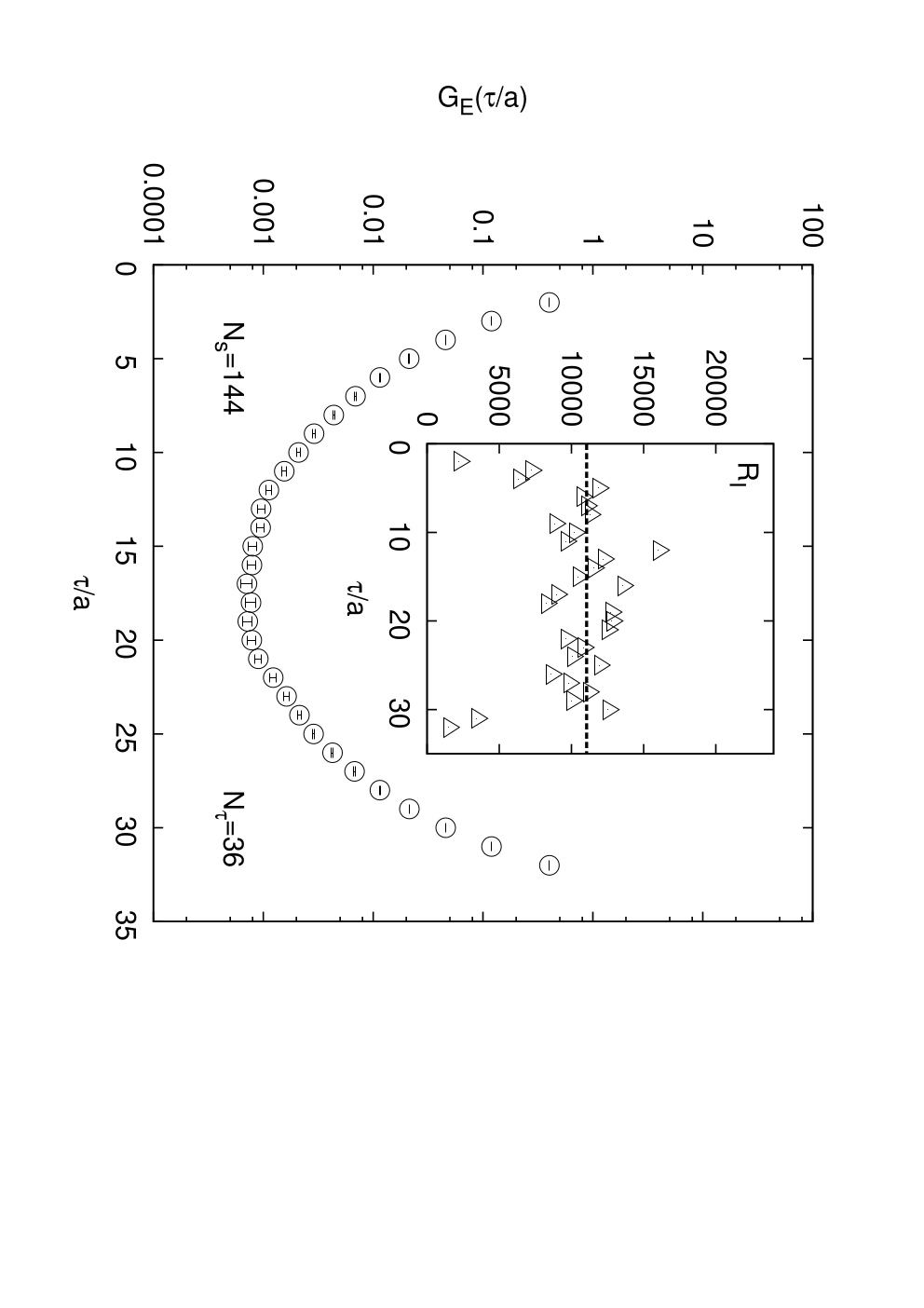
where denotes the colour-electric field, the temperature, and a Wilson line in the Euclidean time direction. A discretized version of this correlator is shown in fig. 3.
Preliminary lattice measurements of the colour-electric correlator have already been carried out [18, 19, 20]. The results look promising, hinting at a large and phenomenologically interesting non-perturbative effect in the diffusion coefficient. However, none of these results contain a systematic continuum extrapolation. The ultimate goal of our investigation is to perform one, by making use of the results of secs. 2, 3 as well as of new simulations.
Our numerical investigations are based on standard lattice QCD techniques. We employ the Wilson gauge action on fine isotropic lattices with lattices spacings down to fm. The measurement of eq. (1) is performed on gauge field configurations generated using 500 sweeps between subsequent configurations, guaranteeing that the configurations are statistically independent. However the correlation function in eq. (1) decreases rapidly with , and for suffers from a weak signal-to-noise ratio. In order to tackle this problem we use a multi-level update [21, 22] for the part of the operator that includes the electric field insertions, and link-integration (“PPR”) [23, 24] for the straight lines between them (the “fat links” in fig. 3). The table in fig. 3 summarizes the situation with labelling the number of statistically independent configurations and the number of additional “multilevel” updates. As demonstrated in fig. 4, these techniques suffice to yield a signal.

| 6.872 | 16 | 32 | 139 | 1000 | 1.111 |
| 6.872 | 16 | 64 | 99 | 1000 | 1.111 |
| 7.192 | 24 | 96 | 159 | 1000 | 1.077 |
| 7.544 | 36 | 144 | 278 | 1000 | 1.068 |
The lattice sizes of our simulations, corresponding to a temperature , substantially exceed those of earlier simulations [18, 19, 20], which had . Due to the increased number of multilevel updates we focussed on lattices with an aspect ratio (cf. the table in fig. 3), which was the optimal choice given the available computational resources. However, volume-scaling checks have been performed at the smallest values of .

After tree-level improvement [8, 22] our measurements yield a correlator denoted by , which is furthermore multiplied by a perturbative renormalization factor [20]. Normalizing the resulting correlator to
| (2) |
the data are displayed in fig. 5. They exhibit a clear enhancement over the next-to-leading order (NLO) prediction from ref. [25]. A continuum extrapolation remains to be carried out.
5 Outlook
The Euclidean correlator of eq. (1) is related to a corresponding spectral function through . Once a perturbatively determined short-distance divergence is subtracted from a continuum-extrapolated , the remainder may be subjected to an analytic continuation algorithm [2, 3] or a well-motivated model like in refs. [19, 20]. In particular, a “momentum diffusion coefficient”, often denoted by , can be obtained from . In the non-relativistic limit (i.e. for , where stands for a heavy quark mass) the corresponding “diffusion coefficient” is given by . It will be interesting to see whether preliminary estimates of the diffusion coefficient [19, 20] can be confirmed after a continuum limit, and how well the results perform in phenomenological comparisons with LHC heavy ion data (cf. e.g. ref. [26]). Of course, taking the continuum limit plays an important role in the extraction of the light-quark diffusion coefficient and electrical conductivity as well [27, 28].
Acknowledgment
This work has been supported in part by the DFG under grant GRK881, by the SNF under grant 200021-140234, and by the European Union through HadronPhysics3 and ITN STRONGnet (grant 238353). Simulations were performed using JARA-HPC resources at the RWTH Aachen (project JARA0039), JUDGE/JUROPA at the JSC Jülich, the OCuLUS Cluster at the Paderborn Center for Parallel Computing, and the Bielefeld GPU cluster.

References
- [1] H.B. Meyer, Eur. Phys. J. A 47 (2011) 86 [1104.3708].
- [2] G. Cuniberti et al, Commun. Math. Phys. 216 (2001) 59 [cond-mat/0109175].
- [3] Y. Burnier, M. Laine and L. Mether, Eur. Phys. J. C 71 (2011) 1619 [1101.5534].
- [4] B. Beinlich, F. Karsch, E. Laermann and A. Peikert, Eur. Phys. J. C 6 (1999) 133 [hep-lat/9707023].
- [5] B. Lucini, M. Teper and U. Wenger, JHEP 01 (2004) 061 [hep-lat/0307017].
- [6] J. Langelage et al, JHEP 02 (2011) 057 [Erratum-ibid. 07 (2011) 014] [1010.0951].
- [7] X. Cheng and E.T. Tomboulis, Phys. Rev. D 86 (2012) 074507 [1206.3816].
- [8] R. Sommer, Nucl. Phys. B 411 (1994) 839 [hep-lat/9310022].
- [9] S. Necco, Nucl. Phys. B 683 (2004) 137 [hep-lat/0309017].
- [10] M. Lüscher, JHEP 08 (2010) 071 [1006.4518].
- [11] M. Guagnelli et al. [ALPHA Collaboration], Nucl. Phys. B 535 (1998) 389 [hep-lat/9806005].
- [12] S. Necco and R. Sommer, Nucl. Phys. B 622 (2002) 328 [hep-lat/0108008].
- [13] S. Dürr, Z. Fodor, C. Hoelbling and T. Kurth, JHEP 04 (2007) 055 [hep-lat/0612021].
- [14] S. Capitani, M. Lüscher, R. Sommer and H. Wittig, Nucl. Phys. B 544 (1999) 669 [hep-lat/9810063].
- [15] N. Brambilla et al, Phys. Rev. Lett. 105(2010)212001 [Erratum-ibid. 108(2012)269903] [1006.2066].
- [16] J. Casalderrey-Solana and D. Teaney, Phys. Rev. D 74 (2006) 085012 [hep-ph/0605199].
- [17] S. Caron-Huot, M. Laine and G.D. Moore, JHEP 04 (2009) 053 [0901.1195].
- [18] H.B. Meyer, New J. Phys. 13 (2011) 035008 [1012.0234].
- [19] D. Banerjee, S. Datta, R. Gavai and P. Majumdar, Phys. Rev. D 85 (2012) 014510 [1109.5738].
- [20] A. Francis, O. Kaczmarek, M. Laine and J. Langelage, PoS LATTICE 2011 (2011) 202 [1109.3941].
- [21] M. Lüscher and P. Weisz, JHEP 09 (2001) 010 [hep-lat/0108014].
- [22] H.B. Meyer, Phys. Rev. D 76 (2007) 101701 [0704.1801].
- [23] G. Parisi, R. Petronzio and F. Rapuano, Phys. Lett. B 128 (1983) 418.
- [24] P. de Forcrand and C. Roiesnel, Phys. Lett. B 151 (1985) 77.
- [25] Y. Burnier, M. Laine, J. Langelage and L. Mether, JHEP 08 (2010) 094 [1006.0867].
- [26] W.M. Alberico et al, Eur. Phys. J. C 73 (2013) 2481 [1305.7421].
- [27] H.-T. Ding et al, Phys. Rev. D 83 (2011) 034504 [1012.4963].
- [28] Y. Burnier and M. Laine, Eur. Phys. J. C 72 (2012) 1902 [1201.1994].