Supernova Relic Neutrino Search with Neutron Tagging at Super-Kamiokande-IV
Abstract
A search for Supernova Relic Neutrinos ’s is first conducted via inverse-beta-decay by tagging neutron capture on hydrogen at Super-Kamiokande-IV. The neutron tagging efficiency is determined to be , while the corresponding accidental background probability is %. Using 960 days of data, we obtain 13 inverse-beta-decay candidates in the range of between 13.3 MeV and 31.3 MeV. All of the observed candidates are attributed to background. Upper limits at 90% C.L. are calculated in the absence of a signal.
Keywords:
Neutron tagging; Water Cherenkov detector; hydrogen; Supernova Relic Neutrinos1 Introduction
Neutrinos emitted from all past core-collapse supernovae should form an isotropic flux. Sometimes called the Diffuse Supernova Neutrino Background (DSNB), these neutrinos will be referred to as Supernova Relic Neutrinos (SRN) herein. Many models have been constructed to predict the SRN flux and spectrum [1, 2, 3, 4, 5, 6, 7, 8, 9, 10, 11, 12]. Although all six types of neutrinos are emitted from a core-collapse supernova, SRN’s are most likely detected via the inverse beta decay (IBD) reaction in existing detectors. Super-Kamiokande (SK) has previously carried out searches for SRNs from the expected IBD positrons without requiring the detection of a delayed neutron, placing an integral flux limit for MeV () in the absence of a signal [14, 15]. Since the detector cannot directly differentiate electrons from positrons (the positron annihilation signal is below Cherenkov threshold in water), these searches suffer from background of electrons and positrons. Some of these potential backgrounds include atmospheric neutrino and charged-current interactions and atmospheric neutrino neutral-current interactions. Many background channels either do not produce neutrons or more than one neutron, but they can generate an electron or positron that passes all of the selection criteria, thereby contaminating the candidate samples. Spallation backgrounds have limited the lower anti-neutrino energy threshold in previous SRN searches at SK.
Positive identification of ’s by tagging (and counting) neutrons in delayed coincidence will play a critical role in both the suppression of backgrounds in those samples as well as in lowering the energy threshold. Kamland made the first attempt to search for the SRN flux down to 8.3 MeV by detecting IBDs with neutron capture on hydrogen in a one-kiloton liquid scintillator detector [13]. This paper will present a study to detect IBDs with neutron capture on hydrogen at SK, providing an improved search of SRNs from the previous threshold of 17.3 MeV down to the present 13.3 MeV, where greater SRN flux is expected. In addition, this study can be treated as an after-the-fact approach in parallel to the ongoing RD initiative aimed at detecting IBDs in water with enhanced neutron captures on dissolved gadolinium.
2 Experimental approaches to detect the neutron
To detect the neutron signal, two independent approaches have been proposed to implement this capability in the SK experiment, a large underground water Cherenkov detector containing 50 kilotons of pure water. The detector consists of a cylindrical inner volume viewed by 11,129 inward-facing 50-cm diameter photomultiplier tubes (PMTs), surrounded by an outer annular volume viewed by 1,885 outward-facing 20-cm PMTs. More detailed descriptions of the detector can be found elsewhere [16]. The first approach [17] involves doping the water with a water-soluble chemical compound of gadolinium, neutron capture on which yields a gamma cascade with a total energy of about 8 MeV. These relatively high energy -rays should be readily seen by SK. The second approach is to detect the single 2.2 MeV released from neutron capture on hydrogen [18]. This approach requires a 500-s forced trigger scheme following a normal trigger, in order to identify the 2.2 MeV offline.
The detection of delayed-coincidence 2.2 MeV ’s was first successfully demonstrated in SK using forced triggers [19]. In the summer of 2008, SK’s front-end electronics were upgraded, after which began the data-taking period known as SK-IV. A major part of this upgrade was to use a 60 kHz periodic trigger to seamlessly read out all PMTs all the time. In this data stream, events are searched for by a software trigger, which is based on the number of coincident PMT hits within 200 ns. To search for delayed-coincidence 2.2 MeV ’s, a new coincidence level was introduced: a super-high-energy (SHE) event requires at least 70 coincident PMT hits corresponding to about 10 MeV (this level was lowered to 58 or about 8 MeV in the summer of 2011). SHE events contain all PMT hits from 5 s before the SHE trigger time to 35 s afterwards. The 5 s of data prior the SHE trigger time provides a chance to catch pre-activity events, e.g. a prompt -ray in a sub-Cherenkov muon background event produced by an atmospheric interaction with oxygen. SHE events without coincident outer detector activity are always followed by an after trigger (AFT) which contains all PMT hits of the subsequent 500 s. The SK-IV data set used in this analysis was taken from November 22, 2008, to December 27, 2011, with a total livetime of 960 days.
3 The IBD event selection
The IBD candidate search can be divided into two steps: one to find the prompt signal with an energy ranging from 12 to 30 MeV in the SHE trigger data; the other to tag the IBD signal through the detection of a delayed event shortly after a prompt event is found. The timing window for the delayed event ranges from 2 to 535 s following the prompt event. To avoid PMT signal reflection at the SK front-end electronics after an event, the delayed event search starts two s after the prompt event time (defined by a GPS-synchronized clock). The prompt events are selected by applying a number of cuts to suppress muon-induced spallation background, atmospheric neutrinos, solar neutrinos, and low energy radioactivities. Details of the selection criteria for the prompt events, such as the spallation cut, pre/post activity cut etc, can be found in [15]. Unlike the analysis in [15], the reconstructed Cherenkov angle is required to be greater than 38 and less than 50 degrees. Also, the solar cosine angle cut of [15] is loosened to 0.9 for energies below 16 MeV because of neutron tagging. The number of remaining solar neutrino events in the sample is estimated to be about two events. Table 1 gives a summary of the event selection. Most efficiencies are evaluated using Monte Carlo (MC) simulation except for that of the spallation cut. The overall systematic uncertainty of the primary event efficiency is 3.3% due to uncertainties in the IBD cross section (1.0%), and the data reduction (3.1% as given in [15]), which are added in quadrature.
| Cuts | (%) | |
|---|---|---|
| First reduction | 49288 | 99.220.04 |
| Spallation cut | 2417 | 86.020.18 |
| External event cut | 2148 | 82.360.19 |
| Solar cut | 1649 | 81.540.20 |
| Cherenkov angle cut | 996 | 75.170.22 |
| Pre/post activity cut | 959 | 75.060.22 |
| cut | 948 | 74.320.22 |
| Multi-ring cut | 943 | 73.640.22 |
| cut | 942 | 73.140.23 |
An average 2.2 MeV event in SK produces about seven recorded PMT hits, all of which share a common orientation in both time and space, but most of the hits have various arrival times due to the different travel distances. The flat timing distribution for these signal hits can be sharpened to form a timing peak if the common orientation or vertex is known. However, the continuous 50 MHz dark noise and radioactive background for all the PMTs render a stand-alone reconstruction very difficult because of the long neutron lifetime. Fortunately, since neutrons produced in IBD quickly thermalize and are eventually captured by hydrogen with a mean free path length of 50 cm, to a good approximation the location for an emission of a 2.2 MeV can be treated to share a common vertex with the prompt event, for which the reconstructed position resolution is 4050 cm. The reconstructed vertex for the prompt event is therefore used to calculate the path length to each hit PMT, in order to subtract the time-of-flight (TOF) from the measured light arrival time. Due to a PMT timing resolution of 3 ns, the hits of real signal events cluster within a 10 ns window, while hits due to PMT dark noise, radioactivity in the surrounding rock, radon contamination events in water, and so on are typically more spread out since the light does not originate from the primary event vertex. A 10 ns sliding window is then applied to search for every timing peak and to give the number of PMT hits (N10). Fig. 1 shows the distribution of N10 for a 2.2 MeV signal and background, in which the signal events are from Monte Carlo simulation, while the background events are from the random trigger data.
To remove background PMT hits the following selection criteria are applied:

The number of PMT hits in N10 is required to be greater than 7. It is noted that about 86% of low energy background events originating near the detector wall have clustered PMTs in both space and time, and thus survive the N10 cut. The number of PMT hits in clusters (N) is defined for those within 10 ns and less than as seen from the positron candidate vertex. A cut on the quantity of NN is required to be greater than 5. Since most of the light of a 2.2 MeV gamma originates from a single Compton electron, most hits are in the same detector hemisphere, while PMT noise is distributed more uniformly. As a result, a summed vector is calculated for all the hits in N10. Angles between the individual vector for each hit and the summed vector are computed, giving the number of hits with an angle greater than (N). The delayed event should be NN 6, which removes events with many background hits in the backward hemisphere. Some PMTs are more likely to be illuminated than others for a given vertex. A hit probability of the i-th PMT is defined by , where is the distance from the vertex to the i-th PMT, is the incident angle, includes the angular dependence of PMT geometry and reflection/absorption of acrylic case, and is the attenuation length of Cherenkov light in the SK water. The calculated hit probabilities for all the hits are sorted in decreasing order. The number of hits accounting for the bottom 25-50% of the summed probabilities is defined as N. The fraction varies with the vertex location and is set to 50% when the vertex is close to the wall. A cut on NN is required to be greater than 4. The final reduction utilizes a likelihood ratio based on four discriminating variables: number of PMT hits within 150 ns around N10 peak, root mean square of the N10 timing peak, root mean square of the azimuth angles for all the PMT hit vectors along the summed vector, and mean value of opening angle between the PMT hit vectors and the summed vector. The likelihood ratio is required to be greater than 0.35.
Table 2 gives a summary for the selection criteria, the background probability, and the efficiency of the delayed events for each cut. The efficiency of the delayed event is corrected with a factor of 92% due to the 533 s time window. It is observed that most delayed events cannot fire sufficient PMTs to meet the minimum requirement on N10.
| Cuts | Bkg Prob. (%) | Efficiency(%) |
|---|---|---|
| N 7 | 100 | 30.190.04 |
| NN 5 | 25.480.04 | 28.270.04 |
| NN 6 | 21.130.04 | 26.780.04 |
| NN 4 | 4.140.02 | 19.110.04 |
| Likelihood ratio 0.35 | 1.060.01 | 17.740.04 |
Basing the TOF correction on the SRN candidate vertex (rather than the true vertex of the delayed event) changes the efficiency of finding delayed events by at most 2.5% relatively. Uniformity of both the MC signal efficiency and the background probability were studied using 110 positions within the detector. These spatial variations of MC signal efficiency and background probability were found to be 5.9% and 16.8%, respectively. These variations were then assigned to the systematic uncertainties. Therefore, the efficiency and the background probability for the delayed events are and %, respectively. Combining the primary event efficiency and delayed event efficiency, the IBD detection efficiency () is obtained to be %.
4 Test with Am/Be source data
To verify the detection efficiency for the 2.2 MeV ’s given in Table 2, a test was carried out using an Am/Be source embedded in a bismuth germanate (BGO) scintillator during SK-IV. The experimental setup and other details can be found elsewhere [19]. The experimental apparatus was deployed at certain positions in the SK tank, during which the forced trigger gate for catching the 2.2 MeV ’s was temporarily enlarged to 800 s in order to obtain a more complete neutron lifetime spectrum. To get the time distribution of the source-related background and accidental background, 10 Hz of 800s random trigger data was also taken. Fig. 2 shows the distribution of time differences (T) between the delayed events and the prompt events, which is fitted with an exponential plus a constant with the signal fraction as a free parameter, to give the neutron lifetime in water. In order to verify the neutron lifetime time and examine possible position dependence of detection efficiency, the source was deployed at three different locations: at the center of the tank, close to the wall, and close to the top. All of the resulting lifetime measurements were consistent within one standard deviation. The average neutron lifetime in water was found to be ()s. The efficiencies measured at the three locations are in agreement within 10%, which also agrees with the estimation of Monte Carlo simulation. The average efficiency of % in this enlarged 800 s window is in good agreement with the value of % estimated from MC simulation.

5 Analysis and Results
Returning to the low energy SRN search using 960 live days of SK-IV data, after passing the selection criteria for both the prompt events and the delayed events the relevant distributions for the remaining events with at least one neutron candidate are shown in Fig. 3. There are 13 IBD candidates observed consistent with accidental background events evaluated to be . Two out of these 13 primary events with electron energies around 12 MeV are observed to have two neutron candidates, which indicates they are likely to be from spallation backgrounds with high neutron multiplicity.
A number of studies have been performed to provide insight into the origin of possible background in this energy domain, especially those arising from atmospheric CC interaction, production and NC interactions with water. This is achieved by changing the cut on the Cherenkov angle of the primary event, in which an electron/positron is defined with . The and events are defined with , while the NC events are defined with . There are 144 primary and candidate events with 22 delayed candidates and 489 NC candidate events with 47 delayed candidates. A clear neutron lifetime curve is observed in both delayed candidate samples, showing that the primary events are indeed accompanied by neutrons. The flat timing offset distribution for the delayed candidates in Fig. 3 does not show significant leakage from these two types of physical backgrounds. The number of atmospheric events is estimated to be 0.1, while the number of the events is about 1.0. The later is due to the charged-current interaction, which produces a delayed neutron and a positron from an invisible Michel decay. In absence of a significant signal the Rolke method [20] is used to convert the number of observed and expected background events and to a 90% C.L upper limit of 80.1 events in total or 30.5 events/22.5 (ktonyear), taking into into account the IBD detection efficiency . Table 3 lists the expected number of SRN events in 22.5 ktonyear for different models. The upper limit on the SRN flux can be derived from using the following simple relation:
| (1) |
where (cm-2s-1) is the total flux for a certain model and is the predicted annual event rate in the energy range which can be found in Table 3. This table also contains upper limits () at 90% C.L. for different models and the predicted annual event rate () after efficiency correction.
| SRN model | ||||
|---|---|---|---|---|
| Constant SN [1] | 52.3 | 10.8 | 1.4 | 147.5 |
| HBD 6 MeV [10] | 21.8 | 4.4 | 0.6 | 150.9 |
| Chemical evolution [4] | 8.5 | 1.5 | 0.2 | 172.6 |
| Heavy metal [5, 6] | 31.3 | 4.7 | 0.6 | 201.8 |
| LMA [7] | 28.8 | 4.2 | 0.5 | 208.8 |
| Failed SN [9] | 12.0 | 1.7 | 0.2 | 214.9 |
| Cosmic gas [3] | 5.3 | 0.7 | 0.1 | 230.6 |
| Star formation rate [8] | 18.7 | 1.8 | 0.2 | 316.3 |
| Population synthesis [2] | 42.1 | 1.3 | 0.2 | 986.1 |

Model-independent differential flux upper limits with one MeV energy bins are also calculated. The 90% C.L upper limits are calculated by
| (2) |
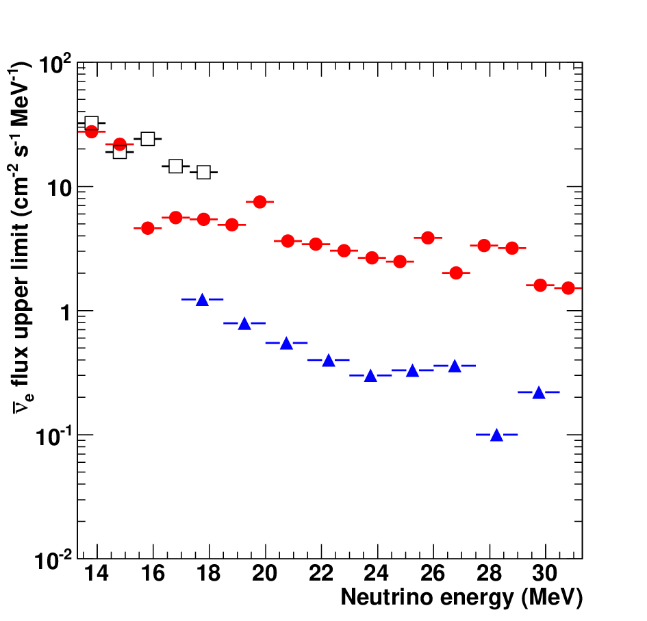
where is the upper limit at 90% C.L. in each energy bin, is livetime in seconds, is the number of free protons, is the average cross section for IBD at the center of each energy bin, and is the IBD detection efficiency for each energy bin. Fig. 4 shows the upper limits for in the energy range of 13.331.3 MeV. Limits from KamLAND [13] based on 2343 live-days are also shown for comparison.
The previous SK search for SRN IBD positrons in [15] placed an integral 90% C.L. limit on the SRN flux above 17.3 MeV neutrino energy of 2.9 cm-2s-1 (LMA model [7]). In that search, SRN signal and atmospheric neutrino backgrounds were fitted to the energy spectra of the data for three different samples differentiated by the reconstructed Cherenkov angle with an extended unbinned maximum likelihood method. The SRN signal populates the single electron-like sample () below 30 MeV (signal region). Various types of atmospheric neutrino background dominate the background region above 30 MeV as well as the other two (background) samples. To compare with the SK-IV differential limits in this paper, the previous SK background spectra as well as the SRN candidate positron spectra above 30 MeV (total energy) were fit to only atmospheric neutrino background contributions. The resulting background fit was extrapolated in the signal region between 16 and 29.5 MeV (total positron energy) taking into account statistical and systematic uncertainties. The data was divided into nine bins of 1.5 MeV. Fig. 4 shows the 90% C.L. upper flux limits derived for each bin based on the background expectations with Gaussian uncertainties and the IBD cross section evaluated at the bin center. Below 17.3 MeV spallation background increases exponentially, so SRN detection in that energy range is very difficult without neutron tagging. As the SRN flux per MeV rises with decreasing energy, the region below 17.3 MeV is the most sensitive.
Since this study covers the high end of the solar neutrino spectrum, a solar upper limit at 90% C.L. of the annual event rate is also calculated, giving an estimate of 21.2 events/22.5 ktonyear. This corresponds to , where is the solar flux predicted by the Standard Solar Model [21]. This limit is 20 times more stringent than the previous SK result [22] due to the powerful background reduction provided by neutron tagging. However, note that the limit is an order less stringent than the KamLAND result [13] because of the higher neutrino energy threshold.
6 Summary and outlook
In summary, a search for SRN at SK-IV is first conducted via IBDs by tagging neutron capture on hydrogen. The neutron tagging efficiency is determined to be , while the corresponding accidental background probability is %. No appreciable IBD signal in the distribution of neutron lifetime is found using 960 days of data. The number of observed IBD candidates are consistent with the expected accidental background. A model-independent differential flux upper limit at SK is first derived from the previous 17.3 MeV threshold down to 13.3 MeV of the electron anti-neutrino energy.
With more data collected and after further efforts in suppressing spallation background, it is expected that the neutrino energy threshold can be lowered down to 10 MeV and the better SRN flux limit can eventually be obtained with neutron capture on hydrogen at SK-IV. In addition, intense RD is currently underway towards a gadolinium-enhanced SK. The higher signal detection efficiency and greater background rejection provided by neutron capture on gadolinium, as well as the lowered energy threshold it makes possible, are expected – in the not-too-distant future – to greatly improve SK′s sensitivity and ultimately provide the world’s first observation of the SRN signal.
7 Acknowledgment
The authors gratefully acknowledge the cooperation of the Kamioka Mining and Smelting Company. The Super-Kamiokande detector was built and operated with funds provided by the Japanese Ministry of Education, Culture, Sports and Technology, the United States Department of Energy, and the U.S. National Science Foundation. This work is also supported by the National Natural Science Foundation of China (Grants No.11235006).
8 References
References
- [1] T. Totani and K. Sato, Astropart. Phys. 3, 367 (1995).
- [2] T. Totani, K. Sato and Y. Yoshii, Astrophys. J. 460, 303 (1996).
- [3] R. A. Malaney, Astropart. Phys. 7, 125 (1997).
- [4] D. H. Hartmann and S. E. Woosley, Astropart. Phys. 7, 137 (1997).
- [5] M. Kaplinghat, G. Steigman and T. P. Walker, Phys. Rev. D 62, 043001 (2000).
- [6] L. Strigari, M. Kaplinghat, G. Steigman and T. Walker, JCAP, 0403:007 (2004).
- [7] S.Ando, K.Sato and T. Totani, Astropart. Phys. 18, 307 (2003).
- [8] M. Fukugita and M.Kawasaki, Mon.Not.Roy.Astron.Soc. 340, L7 (2003).
- [9] C. Lunardini, Phys. Rev. Lett. 102, 231101(2009).
- [10] S. Horiuchi, J.F.Beacom and E.Dwek, Phys. Rev. D 79, 083013 (2009).
- [11] F. Vissani and G. Pagliaroli, Astron. Astrophys. 528 (2011)L1.
- [12] K. Nakazato, Phys. Rev. D 88, 083012 (2013).
- [13] A. Gando et al. (KamLAND Collaboration), Astrophys.J. 745(2012)193.
- [14] M. Malek et al. (Super-Kamiokande Collaboration), Phys. Rev. Lett. 90, 061101(2003).
- [15] K. Bays et al. (Super-Kamiokande Collaboration), Phys. Rev. D 85, 052007 (2012).
- [16] Y. Fukuda et al. (Super-Kamiokande Collaboration), Nucl. Instrum. Meth. A501 (2003) 418-462.
- [17] J. F. Beacom and M. R. Vagins, Phys. Rev. Lett., 2004, 93: 171101.
- [18] S. Chen and Z. Deng, Nucl. Phys. B Proc. Suppl., 2007, 166: 252.
- [19] H. Watanabe et al. (Super-Kamiokande Collaboration), Astropart. Phys., 2009, 31: 320.
- [20] W. A. Rolke, A. M. Lopez and J. Conrad, Nucl. Instrum. Meth. A551 (2005) 493-503.
- [21] J. N. Bahcall and M. H. Pinsonneault, Phys.Rev.Lett., 2004, 92 121301.
- [22] Y. Gando et al. (Super-Kamiokande Collaboration), Phys.Rev.Lett., 2003, 90: 171302.