A Bayesian approach to sparse channel estimation in OFDM systems

Sparse channel estimation is an important topic found in many different applications (see e.g [1, 2, 3, 4, 5] and the references therein). In fact, in many real-world channels of practical interest, e.g. underwater acoustic channels [6], digital television channels [7], and residential ultrawideband channels [8], the associated impulse response tends to be sparse. To obtain an accurate channel impulse response is crucial since it is used in the decoding stage. Sparsity helps one can obtain better channel estimates. In addition, the most common technique for promoting sparsity is by an $\ell_{1}-$norm regularization, commonly termed as Lasso [9]. However, sparsity can be promoted in different ways. For example, in [10], sparsity is promoted by generating a pool of possible models, and then performing model selection.

A special characteristic of OFDM systems is its sensitivity to frequency synchronizations errors (see e.g. [12]), which is produced (among other causes) by carrier frequency offset (CFO). This adds an extra difficulty to the channel estimation problem, since the CFO must be estimated as well as other channel parameters. To estimate the CFO, Maximum Likelihood (ML) estimation has been successfully utilized (see e.g. [25, 11, 12]).

In this work, we combine the following problems: (i) estimation of a sparse channel impulse response (CIR) in OFDM systems, (ii) estimation of CFO, (iii) estimation of the noise variance, (iv) estimation of the transmitted symbol, and (v) estimation of the (hyper) parameter defining the prior probability density function (pdf) of the sparse channel. The estimation problem is solved by utilizing a generalization of the EM algorithm (see e.g. [11, 12, 13, 17] and the references therein) for MAP estimation, based on the $\ell_{1}-$norm of the CIR. In particular, the same methodology has been applied in [17] for the identificaton of a sparse finite impulse response filter with quantized data. Our work generalizes previous work on joint CFO and CIR estimation, see [11] and the generalization [13].

The problem of estimating a sparse channel and the transmitted symbol has been previously addresses in the literature [14]. In [14], it is also considered bit interleaved coded modulation (BICM) in OFDM systems. The approach in [14] corresponds to the utilization of the generalized approximate message passing (GAMP) algorithm [15], which allows for solving the BICM problem. GAMP corresponds to a generalization of the approximate message passing (AMP) algorithm [16], although it does not allow for unknown parameters other than the channel. The AMP and GAMP algorithms are based on belief propagation [15, 16]. When the system is linear (with respect to the channel response), GAMP and AMP are the same algorithm [15]. In addition, for sparsity problems, the AMP algorithm corresponds to an efficient implementation of the Lasso estimator, see[15] and the references therein. Hence, under the same setup, the MAP-EM algorithm we propose and the GAMP algorithm utilized in [14] yield the same results.

We consider the following OFDM system model (see e.g. [12, 13] and the references therein), depiected in Fig. 1 [12]:

• • The channel is modelled as a finite impulse response (FIR) filter $\textbf{h}=[h_{0}\,\,h_{1}\,\,\ldots\,\,h_{L-1}]^{T}\in\mathbb{C}^{L}$ with $L$ taps.

  • CFO is modelled by $\textbf{C}_{\varepsilon}=\exp\{j\mathrm{diag}\left(\frac{2\pi\varepsilon k}{N_{C}}\right)\}$, with $k=0,1,\ldots,N_{C}-1$; $\varepsilon$ is the normalized frequency offset ($|\varepsilon|\leq 1/2$, $N_{C}$ is the number of subcarriers).

  • The cyclic prefix (CP) is removed at the receiver. Thus, the received signal is given by

  $$\textbf{r}=\textbf{C}_{\varepsilon}\tilde{\textbf{H}}{\sf P}\textbf{x}+\boldsymbol{\eta},\vskip-2.84526pt$$

  (1)

  where the channel matrix $\tilde{\textbf{H}}$ is an $(N_{C}\times N_{C})$ circulant matrix whose first column is given by $[h_{0},\,\,h_{1},\,\,\cdots\,\,$ $h_{L-1},\,\,0\,\,\dots\,\,0]^{T}$, x is the transmitted signal (after the inverse discrete Fourier transform), $\sf P$ is a permutation matrix that shuffles the transmitted symbol samples in any desired fashion [12], $\boldsymbol{\eta}\sim{\mathcal{N}}(0,\sigma^{2}{\bf I}_{N_{C}})$, and ${\bf I}_{N_{C}}$ is the identity matrix of dimension $N_{C}$. Notice that the time-domain representation of the multicarrier signals in (1) resembles a single-carrier system. However, the main difference corresponds to the utilization of the cyclic prefix, which yields a circulant channel matrix at the receiver after the cyclic prefix removal.

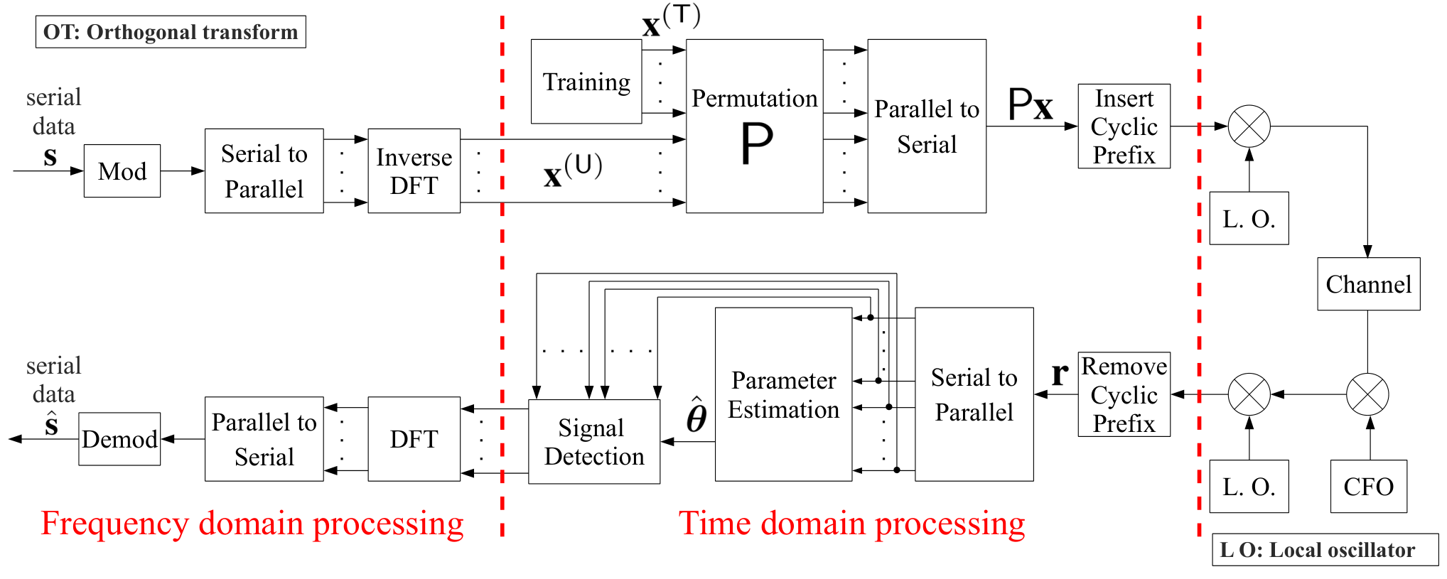
The transmitted signal is assumed to have a deterministic part (comprising known training data) and a stochastic part (comprising the unknown data). Thus, the transmitted signal corresponds, after the application of the IDFT, to the time domain multiplexing of a training sequence and data coming from the data terminal equipment. We also need to express the transmitted signal in terms of the known (training) component, $\textbf{x}^{(\mathsf{T})}$, and the unknown component, $\textbf{x}^{(\mathsf{U})}$. Thus, the real representation of the transmitted signal x is given by

where $(\cdot)_{\text{\textscr}}$, $(\cdot)_{\text{\textsci}}$, $(\cdot)^{\mathsf{(T)}}$ and $(\cdot)^{\mathsf{(U)}}$ represent the real part, imaginary part, training part, and unknown part, respectively.

For estimation purposes, it is possible to express the model in (1) as a real-valued state-space model with sample index $k$:

where $\bar{\textbf{y}}_{k}=[\mathfrak{Re}\left\{r_{k}\right\}\,\mathfrak{Im}\left\{r_{k}\right\}]^{T}$, $\bar{\boldsymbol{\eta}}_{k}=[\mathfrak{Re}\left\{\eta_{k}\right\}\,\mathfrak{Im}\left\{\eta_{k}\right\}]^{T}$, $k=0,1,...,N_{C}-1$ is the time sample index of the OFDM symbol, $\mathfrak{Re}\left\{\cdot\right\}$ and $\mathfrak{Im}\left\{\cdot\right\}$ denote the real and imaginary parts, respectively,

and $\textbf{q}_{k}$ is the $k$th column of the identity matrix. This state-space representation is equivalent to (1), but it is more convenient for the identification approach used in this work. In addition, and as it will be shown in Section 3.2, the estimation procedure is based upon expressions in the form of $E[\bar{\textbf{x}}^{(\sf U)}|\bar{\textbf{y}}]$ and $E[\bar{\textbf{x}}^{(\sf U)}{\textbf{x}^{\mathsf{(U)}}}^{T}|\bar{\textbf{y}}]$, amongst other quantities. The attainment of these two expectations can be achieved, for instance, by applying Bayes’ rule for the posterior pdf

for any given prior pdf $p(\textbf{x}^{\mathsf{(U)}})$.

Regarding the received signal, the conditional pdf of $\textbf{y}=[\bar{\textbf{y}}^{T}_{0},\dots,\bar{\textbf{y}}^{T}_{N_{C}-1}]^{T}$ is given by $p(\textbf{y}\,|\,\boldsymbol{\chi},{\boldsymbol{\theta}})\sim\mathcal{N}(\textbf{M}\bar{\textbf{x}},\boldsymbol{\Sigma}_{y})$ where the vector of parameters $\boldsymbol{\theta}=(\bar{\textbf{h}},\varepsilon,\sigma)$, $\bar{\textbf{h}}=[\mathfrak{Re}\left\{\textbf{h}\right\}\,\mathfrak{Im}\left\{\textbf{h}\right\}]^{T}$, and

with $\hat{\boldsymbol{\eta}}=[\bar{\boldsymbol{\eta}}_{0}^{T}\,\cdots\,\bar{\boldsymbol{\eta}}_{N_{C}-1}^{T}]$. For proper additive white noise with variance $\sigma^{2}$, $\boldsymbol{\Sigma}_{y}=0.5\sigma^{2}{\bf I}_{2N_{C}}$. For the unknown part of the transmitted signal, the corresponding pdf is simply expressed as $p(\bar{\textbf{x}}^{(\sf{U})})$. This allows the transmitted signal to be generated by any modulation scheme, yielding a family of possible pdf’s.

To promote sparsity in the parameter $\bar{\textbf{h}}$, we include an $\ell_{1}$ regularization term in the form of a prior distribution, $p(\bar{\textbf{h}})$, which, in turn, leads to a MAP estimation problem. In general, MAP estimation allows for the inclusion of one or more terms that account for statistical prior knowledge of the parameters $\boldsymbol{\theta}$. However, here we are interested in utilizing prior knowledge of the channel impulse response only. On the other hand, in a MAP estimation problem, a good estimate $\hat{\sigma}$ is crucial. Thus, it is important to take into account $\sigma$ in the definition of the problem (see e.g. [26]). If this is not done, the regularized optimization problem may be non-convex and exhibit numerical difficulties. To address this issue, we can express the prior distribution for $\bar{\textbf{h}}$ as

Since we assume no prior knowledge for the channel noise variance nor the CFO, we choose non-informative marginal prior distributions, for example, $p(\sigma)=p(\epsilon)=1$ (see [26]). Then, the maximization problem becomes

where $p(\textbf{y}|\boldsymbol{\theta})$ is the likelihood function.

To achieve convexity, we now can use the procedure suggested in [26]. That is, we introduce the following reparametrization: $\textbf{\textscg}=\bar{\textbf{h}}/\sigma$, $\rho=\sigma^{-1}$. We therefore define a new parameter to be estimated: $\boldsymbol{\gamma}=(\textbf{\textscg},\varepsilon,\rho)$. Using the new parametrization, and looking at the second term of the right hand side of (11), this term can expressed as a function of \textscg (or equivalently of the “individual” terms of \textscg, $\text{\textscg}_{j}$ is the $j$th element of \textscg, $j=1,2,...,2L$, as (see e.g. [22])

where $z(\cdot)$ is a function specifying the log-prior.

In this section, we present a numerical example using our approach for an OFDM system with CFO. We assume that the unknown part of the time-domain transmitted signal is approximately Gaussian distributed (a consequence of the Central Limit Theorem). Thus, $p(\bar{\textbf{x}}^{(\sf{U})})\sim\mathcal{N}\left(\textbf{0},\boldsymbol{\Sigma}_{\bar{x}^{({\sf U})}}\right)$, where $\boldsymbol{\Sigma}_{\bar{x}^{({\sf U})}}=\begin{bmatrix}\boldsymbol{\Sigma}_{\textbf{x}_{\text{\textscr}}^{({\sf U})}}&\boldsymbol{\Sigma}_{\textbf{x}_{\text{\textscr}}^{({\sf U})}\textbf{x}_{\text{\textsci}}^{({\sf U})}}\\ \boldsymbol{\Sigma}_{\textbf{x}_{\text{\textsci}}^{({\sf U})}\textbf{x}_{\text{\textscr}}^{({\sf U})}}&\boldsymbol{\Sigma}_{\textbf{x}_{\text{\textsci}}^{({\sf U})}}\end{bmatrix}$, $\boldsymbol{\Sigma}_{\textbf{x}_{\text{\textscr}}^{({\sf U})}}=E[\textbf{x}_{\text{\textscr}}^{({\sf U})}{\textbf{x}_{\text{\textscr}}^{({\sf U})}}^{T}]$, $\boldsymbol{\Sigma}_{\textbf{x}_{\text{\textsci}}^{({\sf U})}}=E[\textbf{x}_{\text{\textsci}}^{({\sf U})}{\textbf{x}_{\text{\textsci}}^{({\sf U})}}^{T}]$, and $\boldsymbol{\Sigma}_{\textbf{x}_{\text{\textsci}}^{({\sf U})}\textbf{x}_{\text{\textscr}}^{({\sf U})}}=E[\textbf{x}_{\text{\textsci}}^{({\sf U})}{\textbf{x}_{\text{\textscr}}^{({\sf U})}}^{T}]$ (known).

The expectations on the right hand side of (17) and (18) can be readily calculated by applying Kalman filtering to the model in (8). In addition, we consider that channel noise variance is unknown. We consider the following set-up: (i) $N_{C}=64$, (ii) a sparse channel impulse response of length $20$, with $14$ taps equal to zero, (iii) the transmitted signal is Gaussian distributed, (iv) the signal to noise ratio is $5[\text{dB}]$ and $10[\text{dB}]$, (v) $\varepsilon=0.2537$, and (vi) $62.5\%$ of training. As a performance measure, we consider the normalized mean square error, defined as $\text{NMSE}:=(\textbf{h}-\hat{\textbf{h}})^{H}(\textbf{h}-\hat{\textbf{h}})/(\textbf{h}^{H}\textbf{h})$. Using 100 different realizations for the noise, the results can be seen in Table 1. We can conclude that regularization only helps if limited amount of data is available. For the case of $\text{SNR}=10[\text{dB}]$, in Fig 2, the average BER for ML estimation is 0.0195, and for MAP estimation is 0.0132.

In this work, we have proposed an algorithm to estimate sparse channels in OFDM systems, the CFO, the variance of the noise, the symbol, and the parameter defining the a priori distribution of the sparse channel. This is achieved in the framework of MAP estimation, using the EM algorithm.

Sparsity has been promoted by using an $\ell_{1}$-norm regularization, in the form of a prior distribution for the CIR. For that, the EM algorithm has been modified to include this case. In addition, we have concentrated the cost function in the M-step to numerically optimize one single variable ($\varepsilon$).

The numerical examples illustrate the effectiveness of this approach for the partial training case, obtaining, in most cases studied, a lower value for NMSE using regularization compared to the value for NMSE using no regularization. For the full training case, there is no noticeable difference between the estimates obtained with ML and MAP. This confirms that prior knowledge is useful when the amount of data is limited.

References

- [1] S. F. Cotter and B. D. Rao, “Sparse channel estimation via matching pursuit with application to equalization,” IEEE Trans. Comms., 50(3), pp. 374–377, 2002.
- [2] M. Stojanovic, “Underwater acoustic communication channels: Propagation models and statistical characterization,” IEEE Comms. Mag., 47(1), pp. 84–89, 2009.
- [3] C.R. Berger, S. Zhou, J.C. Preisig, and P. Willett ”Sparse Channel Estimation for Muticarrier Underwater Acoustic Communication: From Subspace Methods to Compressed Sensing,” IEEE Trans. Signal Proc., 58(3), pp. 1708–1721, 2010.
- [4] G. Tauböck and F. Hlawatsch, ”A compressed sensing technique for OFDM channel estimation in mobile environments: Exploiting channel sparsity for reducing pilots,” ICASSP, 2008.
- [5] S. Kim, “Angle-domain frequency-selective sparse channel estimation for underwater MIMO-OFDM systems,” IEEE Comms. Letters, vol. 16, no. 5, pp. 685–687, 2012.
- [6] D.B. Kilfoyle and A.B. Baggeroer, ”The state of the art in underwater acoustic telemetry,” IEEE J. Oceanic Eng.,, 25(1), pp.4-27, 2000.
- [7] Receiver performance guidelines, ”ATSC recommended practices for digital television,” 2004. Available: http://www.stsc.org/standards /practices.html.
- [8] A. F. Molisch, “Ultrawideband propagation channels-Theory, measurement, and modeling,” IEEE Trans. Veh. Tech., 54(5), pp.1528–45, 2005.
- [9] R. Tibshirani, “Regression shrinkage and selection via the lasso,” J. Royal. Statist. Soc B, vol. 58, no. 1, pp. 267–288, 1996.
- [10] E. G. Larsson and Y. Selén, “Linear regression with a sparse parameter vector,” IEEE Trans. Signal Proc., 55(2), pp. 451–460, 2007.
- [11] R. Mo, Y. H. Chew, T. T. Tjhung, and C. C. Ko, “An EM-based semiblind joint channel and frequency offset estimator for OFDM systems over frequency selective fading channels,” IEEE Trans. Veh. Tech., 57(5), pp.3275–3282, 2008.
- [12] R. Carvajal, J. C. Agüero, B. I. Godoy, and G. C. Goodwin, “EM-based channel estimation in Muticarrier systems with phase distortion,” IEEE Trans. Veh. Tech., vol. 62, no. 1, pp. 152-160, 2013.
- [13] R. Carvajal, B. I. Godoy, J. C. Agüero, and G. C. Goodwin, “EM-based sparse channel estimation in OFDM systems,” SPAWC, June 2012.
- [14] P. Schniter, “A message -Passing Receiver for BICM-OFDM over Unknown Clustered-Sparse Channels,” IEEE Journal of Sel. Topics in Sig. Process., vol. 5, no. 8, pp. 1462–1474, 2011.
- [15] S. Rangan, “Generalized approximate message passing for estimation with random linear mixing,” arXiv:1010.5141v2 [cs.IT]., Aug. 2012.
- [16] D. L. Donoho, A. Maleki, and A. Montanari, “Message-passing algorithms for compressed sensing,” Proc. Nat. Acad. Sci., vol. 106, no. 45, pp. 18 914–18919, Nov. 2009.
- [17] B. Godoy, J.C. Agüero, R. Carvajal, G.C. Goodwin, and J.I. Yuz, “Identification of sparse FIR systems using a general quantization scheme,” International Journal of Control, accepted for publication.
- [18] K. S. Miller, Complex stochastic processes: An introduction to theory and applications, London, UK: Addison-Wesley Pub. Co., Inc., 1974.
- [19] S. Buzzi, M. Lops, and S. Sardellitti, “Widely linear reception strategies for layered space-time wireless communications,” IEEE Trans. Signal Proc., 54(6), pp. 2252–2262, 2006.
- [20] Z. Wang, X. Ma, and G. B. Giannakis, “OFDM or single-carrier block transmissions?,” IEEE Trans. Commun., vol. 52, no. 3, pp.380–394, 2004.
- [21] K. Amleh, H. Li, and T. Li, “Robust channel estimation and detection for single-carrier and multicarrier block transmission systems,” IEEE. Trans. Veh. Tech., vol. 59, no. 2, pp. 662–672, 2010.
- [22] N. G. Polson and J. G. Scott, “Data augmentation for non-Gaussian regression models using variance-mean mixtures,” Biometrika, vol. 100, no. 2, pp. 459–471, 2013.
- [23] A. P. Dempster, N. M. Laird, and D. B. Rubin, “Maximum likelihood from incomplete data via the EM algorithm,” J. R. Stat. Soc. B, 39(1), pp. 1–38, 1977.
- [24] O. Barndorff-Nielsen, J. Kent, and M. Sorensen, ”Normal variance-mean mixtures and z distributions,” Int. Stat. Review, 50(2), 1982.
- [25] P.H. Moose, ”A Technique for Orthogonal Frequency Division Multiplexing Frequency Offset Correction,” IEEE Trans. Comms., 42(10), pp. 2908–2914, 1994.
- [26] N. Städler, P. Bühlmann, and S. van de Geer, ”-penalization for mixture regression models,” Test, vol. 19, pp. 209–256, 2010.
- [27] T. Söderström, and P. Stoica, System Identification,” Prentice-Hall, 1989.