Impact of Limpware on HDFS:
A Probabilistic Estimation

Thanh Do Haryadi S. Gunawi

^† University of Wisconsin-Madison

University of Chicago

Abstract

With the advent of cloud computing, thousands of machines are connected and managed collectively. This era is confronted with a new challenge: performance variability, primarily caused by large-scale management issues such as hardware failures, software bugs, and configuration mistakes. In our previous work [2, 3] we highlighted one overlooked cause: limpware – hardware whose performance degrades significantly compared to its specification. We showed that limpware can cause severe impact in current scale-out systems. In this report, we quantify how often these scenarios happen in Hadoop Distributed File System.

1 Introduction

In our latest work [2, 3], we highlight one overlooked cause of performance variability: limpware - hardware whose performance degrades significantly compared to its specification. The growing complexity of technology scaling, manufacturing, design logic, usage, and operating environment increases the occurrence of limpware. We believe this trend will continue, and the concept of performance perfect hardware no longer holds. We have collected reports and anecdotes on cases of limpware. We find that disk bandwidth can drop by 80%, network throughput by two orders of magnitude, and processor speed by 25%. Interestingly, such degraded behavior is exhibited by both commodity as well as enterprise hardware. Our work shows that although today’s scale-out systems employ redundancies, they are not capable of making limpware “fail in place”. Impact of limpware cascades, leading to degraded operation (e.g., a write can degrade to 1KB without trigger a failover), nodes and cluster (e.g., a node or the whole cluster are unable to perform certain task).

In this report, we calculate how often these degraded scenarios happen in HDFS [1]. Although, HDFS employs redundancies for fault-tolerance, its protocols are susceptible to limpware [2, 3]. We specifically look at three protocols (i.e., read, write, and regeneration) and quantify the probability that these protocols experience degraded condition. We further verify our calculation by simulation. Our results show that probabilities of these scenarios are alarmingly high in small and medium (e.g., 30-node) clusters. However, these probabilities reduce significantly when size of cluster increases, as “Scale can be your friend” [4].

This report is structured as follows. We highlight an overview of HDFS in Section 2, present the probability derivation in Section 3, and conclude.

2 HDFS Overivew

We now briefly describe the architecture and main operations of HDFS [1]. HDFS has a dedicated master, the namenode, and multiple workers called datanodes. The namenode is responsible for file-system metadata operations, which are handled by a fixed-size thread pool with 10 handlers by default. The namenode stores all metadata, including namespace structure and block locations, in memory for fast operations.

While the namenode serves metadata operations, the datanodes serve read and write requests. For fault tolerance, data blocks are replicated across datanodes. A new data block is written through a pipeline of three different nodes by default. Therefore, each data block typically has three identical replicas. On read, HDFS tries to serve the request a replica that is closest to the reader.

Since a data block can be under-replicated due to many reasons such as disk and machine failures, the namenode ensures that each block has the intended number of replicas by sending commands to datanodes, asking them to regenerate certain blocks. Block regeneration also happens when a datanode is decommissioned; all of its blocks are regenerated before it leaves. Each datanode allows maximumly two threads serving regeneration request at a time so that regeneration does not affect foreground workload.

3 Probability Derivation

In this section, we first show examples of limpware causing negative impact on three protocols of HDFS: read, write, and regeneration. We then calculate how often such scenarios happen for each protocol.

3.1 Impact of Limpware

Refer to caption — Figure 1: Impact of limpware on HDFS. The figures show the impact of slow network card on three HDFS protocols: read, write and regeneration.

Our previous work [2] shows that HDFS is limpware intolerant. Here, we show examples of HDFS protocols suffering from negative impact of slow network card (NIC). Specifically, we run workloads that exercise three HDFS protocols (read, write, and regeneration), inject slowdown to NIC of a node in the cluster, and measure the resulting execution time. Figure 1 shows the results. The normal bandwidth for the network is 100Mbps. We slow down the NIC to 10, 1, and 0.1Mbps in each experiment. We inject crash to evaluate HDFS fail-stop failure tolerance. In all experiments, HDFS is not able to detect a slow NIC, hence does not trigger a failover. As a result, total execution time in case of slow NIC is orders of magnitude higher than in normal scenario.

These results confirm that HDFS protocols are not able to tolerate limpware. We next quantify how often such negative impacts happen for each protocol, given the cluster’s size, number of data blocks it manages, and number of user requests.

3.2 Degraded Read

$\bullet$ Definition. Consider an $n$ -node cluster which has one slow node $L$ and $n-1$ good nodes. A user request reads data from one out of three copies (assuming 3-way replication) of certain block $B$ . Each copy has an equal chance to be chosen. We define a degraded read to be a read request that reads data the slow node $L$ .

$\bullet$ Derivation. We now derive the probability of a degraded read. There are two conditions for a read of block $B$ to degrade. First, $L$ must contain one copy of $B$ , and second, the copy in $L$ is chosen for reading.

Let’s derive the probability for the first condition. There are ${n\choose 3}$ ways to choose 3 out of $n$ nodes; there are ${n-1\choose 3}$ ways to choose 3 out of $n-1$ good nodes. Therefore, the number of ways to choose 3 nodes, one of which is $L$ , out of $n$ nodes is ${n\choose 3}-{n-1\choose 3}$ . The probability for L to contain one copy of $B$ is:

\begin{split}P(L~contains~one~copy~of~B)=\frac{{n\choose 3}-{n-1\choose 3}}{{n\choose 3}}=\frac{3}{n}\end{split}

(1)

Since there are three copies of $B$ , the probability for the copy in slow node $L$ to be chosen for reading is $\frac{1}{3}$ . As a result, the probability for a read to degrade is:

P(a~read~to~degrade)=p_{rl}=\frac{3}{n}\times\frac{1}{3}=\frac{1}{n}

(2)

Let $r$ be the number of read requests of a user during a certain operation period (e.g., a day). We now derive the probability that the user has at least one degraded read. The probability for a read not to degrade is $1-p_{rl}$ . The probability for all $r$ requests not to degrade is $(1-p_{rl})^{r}$ . As a result, the probability for a user to experience at least one degraded read is:

P(user~has~at~least~one~degraded~read)=P_{rl}=1-(1-p_{rl})^{r}=1-(1-\frac{1}{n})^{r}

(3)

$\bullet$ Result. Figure 2 plots probabilities for a request to degrade ( $p_{rl}$ ) and for a user to experience at least one degraded read ( $P_{rl}$ ). As cluster size increases, these probabilities decrease since there are more healthy nodes.

3.3 Degraded Write

$\bullet$ Definition. Consider an $n$ -node cluster which has one slow node $L$ and $n-1$ good nodes. A user write request requires HDFS to allocate 3 nodes to write to (assuming 3-way replication). Each node has an equal chance to be chosen in a write pipeline. We define a degraded write to be a write request whose pipeline contains $L$ .

$\bullet$ Derivation. We now derive the probability for write to be slow. It is the probability for $L$ to be chosen as one of the nodes in the 3-node write pipeline. We follow the similar derivation as in Section 3.2. There are ${n\choose 3}$ ways to choose 3 out of $n$ nodes; there are ${n-1\choose 3}$ ways to choose 3 out of $n-1$ good nodes. Therefore, the number of ways to choose 3 nodes, one of which is $L$ , out of $n$ nodes is ${n\choose 3}-{n-1\choose 3}$ . Thus, the probability for a write to be degraded is:

P(a~write~to~degrade)=p_{wl}=\frac{{n\choose 3}-{n-1\choose 3}}{{n\choose 3}}=\frac{3}{n}

(4)

Let $r$ be the total number of requests that a user has during a certain working period (e.g., a day). We now derive the formula for the probability that the user experience at least one slow write, $P_{wl}$ . The probability for a write not to be slow is $1-p_{rl}$ . The probability for the user does not have any slow write equals the probability that all $r$ write requests are not degraded, which is $(1-p_{wl})^{r}$ . Therefore, the probability for the user experiences at least one degraded write is:

P(user~has~at~least~one~degraded~write)=P_{wl}=1-(1-p_{wl})^{r}=1-(1-\frac{3}{n})^{r}

(5)

$\bullet$ Result. Figure 3 plots the probabilities for degraded write as function of cluster size and number of user requests. These probabilities are significant larger than those for degraded read, because each write has to be written to a 3-node pipeline. Even in a cluster of 50 nodes, a user is likely to experience one slow write on every 40 requests.

3.4 Degraded Regeneration

3.4.1 Definitions

Consider an HDFS cluster consisting of $n$ datanodes, one of which is slow (node $L$ ). Let $C$ be a node that crashes; there are $n-1$ surviving nodes including the slow one. Let $G$ be the set of good nodes (nodes are neither slow nor crashed); there are $n-2$ good nodes.

Let $b$ be the total number of blocks in node $C$ . When node $C$ crashes, HDFS triggers regeneration workload to regenerate those lost blocks. On average, each surviving node has to replicate $m=\frac{b}{n-1}$ blocks to other live nodes.

m=\frac{b}{n-1}

(6)

For each lost block, the master chooses a source and a destination datanode. The source is chosen from live nodes that still carry the block. The destination node is chosen using the write allocation policy (that uses randomness). A source datanode can only run two regeneration threads at a time.

$\bullet$ Degraded node. Consider a good node $X,X\in G$ . When both regeneration threads of $X$ send blocks to a slow node $L$ , the node is not available for new regeneration tasks until the two threads finish (which could take a long time). We define this situation a degraded node during regeneration process. The situation is illustrated in Figure 4a.

$\bullet$ Degraded cluster. When all good nodes are degraded, as illustrated in Figure 4b, the whole system is unable to start any regeneration task. We define this scenario a degraded cluster. Formally, the cluster degrades during regeneration when $\forall X\in G,X$ degrades.

$\bullet$ Degraded block. The system may not be able to regenerate block $B$ for a long time. This can happen in two cases, which are illustrated in Figures 4c and 4d. First, all remaining copies of $B$ are in degraded nodes (Figures 4c), and second, one copy of B is in a degraded node, the other is in slow node $L$ (Figures 4d). Note that these cases are mutually exclusive and in the illustration, replication threads are copying different blocks other than $B$ .

3.4.2 Derivation

We now derive the probabilities for degraded node, cluster, and block scenarios. To facilitate our calculation, we first derive the probability that node $L$ is destination of a copy task.

$\bullet$ $L$ is destination for a copy task. Consider a scenario where good node $X$ $(X\in G)$ copies one of its blocks (e.g., block $B$ ) to another node. Let $p$ be the probability that $L$ is selected as destination. For this to happen, there are two conditions: first, $L$ does not have a copy of $B$ and second, the master chooses $L$ to be the destination.

We now derive the probability of the first condition. Since $X$ and $C$ both contain a copy of $B$ , the probability for $L$ to also contain $B$ is $\frac{1}{n-2}$ . Therefore, the probability for a copy of $B$ not in $L$ is $1-\frac{1}{n-2}=\frac{n-3}{n-2}$ .

P(copy~of~block~B~in~L)=\frac{1}{n-2}

(7)

P(copy~of~block~B~not~in~L)=1-\frac{1}{n-2}=\frac{n-3}{n-2}

(8)

We calculate the probability that the master chooses $L$ as destination, given that $L$ does not contain $B$ . Note that to the master can only choose one from $n-3$ nodes that do not have a copy of block $B$ . Thus, given $L$ not storing $B$ , the probability for $L$ to be the destination is $\frac{1}{n-3}$ . As a result, the probability for $X$ to copy block $B$ to $L$ is:

p=P(L~is~destination~of~a~copy~task)=\frac{n-3}{n-2}\times\frac{1}{n-3}=\frac{1}{n-2}

(9)

$\bullet$ Degraded node probability. Let $P_{nl}$ be the probability for node $X,X\in G$ degrades during regeneration process. We assume the time to copy a block between two good nodes is inconsiderable compared to the time to copy a block between a good and a slow node $L$ . As a result, $P_{nl}$ is the probability that $X$ copies at least two blocks to $L$ , out of $m$ blocks it has to regenerate.

Since the probability for X not to copy any blocks to L (out of $m$ blocks) is $(1-p)^{m}$ and the probability for X to copy exactly one block to L (again, out of $m$ blocks) is ${m\choose 1}\times p\times(1-p)^{m-1}$ , we have:

\begin{split}P(a~node~degrades)=P_{nl}\\ =1-(1-p)^{m}-{m\choose 1}\times p\times(1-p)^{m-1}\\ =1-(1-\frac{1}{n-2})^{\frac{b}{n-1}}-\frac{b}{(n-1)\times(n-2)}\times(1-\frac{1}{n-2})^{\frac{b-n+1}{n-1}}\end{split}

(10)

$\bullet$ Degraded cluster probability. Let $P_{cl}$ be the probability for the whole cluster to degrade during regeneration. This scenario happens when all good nodes degrade. Therefore:

P(the~cluster~degrades)=P_{cl}={P_{nl}}^{n-2}

(11)

$\bullet$ Degraded block probability. Let $p_{bl}$ be the probability for a block $B$ to be degraded. There are two mutually exclusive cases for this scenario (Figure 4c and Figure 4d). Let the probabilities of these cases are $p_{bl_{1}}$ and $p_{bl_{2}}$ , respectively. Because they are mutually exclusive, we have:

p_{bl}=p_{bl_{1}}+p_{bl_{2}}

(12)

We now calculate probability of the first case, $p_{bl_{1}}$ , the case where all of block $B$ ’s remaining copies are stored in degraded nodes (Figure 4c). Let $i$ be the number of good but degraded nodes. The probability to have exactly $i$ good but degraded nodes is

\begin{split}P(having~i~degraded~nodes)=\\ p_{nl}(i)={n-2\choose i}\times{P_{nl}}^{i}\times(1-P_{nl})^{n-2-i}\end{split}

(13)

For this first case to happen, there are two conditions: (1) $i\geq 2$ ; and (2) two copies of block $B$ are stored among those $i$ nodes. There are ${n-1\choose 2}$ ways to place two copies of $B$ among $n-1$ nodes (excluding the crashed one which must contain $B$ ). There are ${i\choose 2}$ ways to place two copies of $B$ among $i$ degraded nodes. Therefore, the probability for two copies of $B$ be in two (out of $i$ ) degraded nodes is $\frac{{i\choose 2}}{{n-1\choose 2}}$ . As a result:

p_{bl_{1}}(i)=p_{nl}(i)\times\frac{{i\choose 2}}{{n-1\choose 2}},2\leq i\leq n-2

(14)

To calculate the exact value of $p_{bl_{1}}$ , we must consider all possible values of $i$ . Because $i$ can vary from $2$ to $n-2$ , the final equation for the probability of the first case (Figure 4c) is:

p_{bl_{1}}=\sum_{i=2}^{n-2}p_{nl}(i)\times\frac{{i\choose 2}}{{n-1\choose 2}}

(15)

Now, let’s calculate, $p_{bl_{2}}$ , the probability for the second case (Figure 4d), which happens when: (1) $i\geq 1$ ; and (2) one remaining copy of $B$ is in $L$ , and the other is in one (out of $i$ ) good but degraded node. Again, the probability to have exactly $i$ good but degraded nodes is $p_{nl}(i)$ . There are ${i\choose 1}=i$ ways to place two copies of $B$ , one of which in $L$ and the other one in degraded node. Therefore, the probability for two copies of $B$ be in this situation is $\frac{i}{{n-1\choose 2}}$ . As a result:

p_{bl_{2}}(i)=p_{nl}(i)\times\frac{i}{{n-1\choose 2}},1\leq i\leq n-2

(16)

Since $i$ can vary from $1$ to $n-2$ in the second case, we have:

p_{bl_{2}}=\sum_{i=1}^{n-2}p_{nl}(i)\times\frac{i}{{n-1\choose 2}}

(17)

Since two cases for a block to degrade are mutually exclusive, the degraded block probability is:

\begin{split}P(a~degraded~block)=p_{bl}=p_{bl_{1}}+p_{bl_{2}}\\ =\sum_{i=2}^{n-2}p_{nl}(i)\times\frac{{i\choose 2}}{{n-1\choose 2}}+\sum_{i=1}^{n-2}p_{nl}(i)\times\frac{i}{{n-1\choose 2}}\end{split}

(18)

We are now able to calculate the probability for the scenario where at least one block degrades during regeneration process. The probability for a block B not to degrades is $1-p_{bl}$ . The probability of having zero degraded block is $(1-p_{bl})^{b}$ . Therefore, the probability of having at least one degraded block:

\begin{split}P(at~least~one~degraded~block)=\\ P_{bl}=1-(1-p_{bl})^{b}\end{split}

(19)

3.4.3 Results

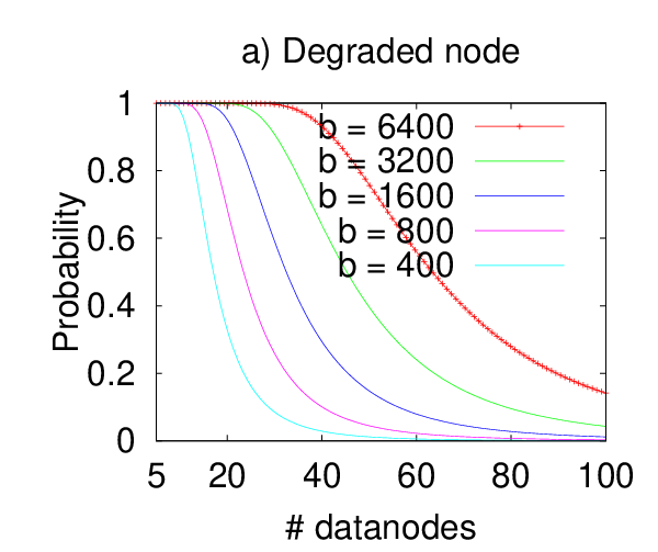
To be more confident with our calculation, we simulate HDFS regeneration protocol and run regeneration workload. We vary the number of nodes in the cluster and the number of lost blocks. We run each configuration (with different cluster size and number of lost blocks) 100 times, and measures the probability of degraded block and degraded cluster.

Figures 5 and 6 show both our calculation and simulation results. Degraded-node and degraded-cluster probabilities are relatively high for a small to medium (e.g., 30-node) cluster. Degraded block probability is alarmingly high: even in a 100-node cluster, a dead 20%-full 1TB node (that can store 3200 blocks) will lead to at least one degraded block. Simulation results are similar to our calculation.

4 Conclusion

Limpware without doubt is a destructive failure mode, yet we show that HDFS fail to properly handle limpware. We present a probabilistic estimation of how often such negative impact of limpware happens to three important HDFS protocols: read, write, and regeneration. Our estimation shows that impact of limpware is significant, even a medium sized cluster of 30-40 nodes.

References

[1] HDFS Architecture. http://hadoop.apache.org/common/docs/current/hdfs_design.html.
[2] Thanh Do and Haryadi S. Gunawi. The case for limping-hardware tolerant cloud. In 5th USENIX Workshop on Hot Topics in Cloud Computing (HotCloud), 2013.
[3] Thanh Do, Mingzhe Hao, Tanakorn Leesatapornwongsa, Tiratat Patana-anake, and Haryadi S. Gunawi. Limplock: Understanding the Impact of Limpware on Scale-Out Cloud Systems. In Proceedings of the 4th ACM Symposium on Cloud Computing (SoCC), 2013.
[4] Diego Ongaro, Stephen M. Rumble, Ryan Stutsman, John Ousterhout, and Mendel Rosenblum. Fast Crash Recovery in RAMCloud. In Proceedings of the 23rd ACM Symposium on Operating Systems Principles (SOSP), 2011.

Impact of Limpware on HDFS: A Probabilistic Estimation