LHC-scale left-right symmetry and unification
Abstract
We construct a comprehensive list of non-supersymmetric standard model extensions with a low-scale LR-symmetric intermediate stage that may be obtained as simple low-energy effective theories within a class of renormalizable GUTs. Unlike the traditional “minimal” LR models many of our example settings support a perfect gauge coupling unification even if the LR scale is in the LHC domain at a price of only (a few copies of) one or two types of extra fields pulled down to the TeV-scale ballpark. We discuss the main aspects of a potentially realistic model building conforming the basic constraints from the quark and lepton sector flavour structure, proton decay limits, etc. We pay special attention to the theoretical uncertainties related to the limited information about the underlying unified framework in the bottom-up approach, in particular, to their role in the possible extraction of the LR-breaking scale. We observe a general tendency for the models without new coloured states in the TeV domain to be on the verge of incompatibility with the proton stability constraints.
Keywords:
Left-right symmetry, LHC; GUTpacs
14.60.Pq, 12.60.Jv, 14.80.CpI Introduction
It is well-known that with only the standard model (SM) field content the gauge couplings do not unify at a single energy scale, while the minimal supersymmetric standard model (MSSM) leads to quantitatively precise gauge coupling unification (GCU), if the scale of supersymmetry is “close” to the electro-weak (EW) scale [1, 2, 3, 4, 5, 6, 7]. 11 1 Actually, within supersymmetric models it is only required that the new fermions (higgsinos, wino and gluino) have masses near the EW scale, as in the so-called “split SUSY” scenario [8, 9]. However, there are many extensions of the SM that lead to GCU without supersymmetry (SUSY). In particular, it is much less known that already in [10] GCU was studied in a number of non-SUSY extensions of the SM. We also mention one particular example with vector-like quarks (VLQ) that was discussed recently in [11], where the Higgs mass and stability bounds and the GCU were considered in an SM extension with two different VLQs.
On the other hand, there are rather few publications which discuss GCU within left-right symmetric extensions of the SM. The main reason for this is probably the fact that for minimal left-right (LR) symmetric extensions of the SM the couplings do not unify unless the LR scale is rather high, say () GeV, as has been shown already in [12].
While for the SM the term “minimal” is unambiguously defined, for LR symmetric extensions of the SM the term “minimal-LR” model has been used for quite different models in the literature. Usually in “minimal LR” models a second SM Higgs doublet is added to the SM field content at the LR scale to complete a bi-doublet, , 22 2 Throughout this paper we will use the notation for scalars and for fermions with the subscript denoting the quantum numbers with respect to either the left-right () or the SM group (). as required by the LR group. To break the LR group to the SM group one then (usually) adds a pair of triplets + [13, 14, 15]. Here the presence of the left-triplet allows to maintain parity in the LR phase, i.e. , sometimes also called “manifest LR” symmetry. This construction automatically also creates a seesaw mass for the right-handed neutrinos from the vacuum expectation value of the [15]. We will call this setup the “minimal LR” (mLR) model in the following. Alternatively, also a pair of doublets, + , could break the LR group for an equally simple setup. However, in this case one would need to rely on an inverse [16] (or linear [17, 18]) seesaw for generating neutrino masses.
In [19] it has been argued that a “truly minimal LR model” has only two doublets + but no bi-doublet. In this case, all fermion masses are generated from non-renormalizable operators (NROs). While this setup has indeed one field less than the above “minimal-LR” models, it needs some additional unspecified new physics to generate the NROs and, thus, can not be considered a complete model. Unification in this “truly minimal” setup is achieved for an LR scale around roughly GeV (and a grand unified theory (GUT) scale of roughly GeV [20].
A LR model with only bi-doublets can not generate the observed Cabibbo-Kobayashi-Maskawa (CKM) mixing angles at tree-level, see the discussion in the next section. This can be solved by adding a second plus a pair of neutral triplets, + . A supersymmetric version of this setup has been discussed in [21, 22], see also [23]. We will call this model the “minimal LR” (mLR) model. Fig. 1 shows the running of the gauge couplings for the minimal setup (“mLR”), including 2-loop beta coefficients, in the left plot and for the mLR model in the right plot. Note, that the best fit point (b.f.p.) for GeV and GeV in the mLR model, while the b.f.p. for GeV and GeV in the mLR model.33 3 The authors of [21, 22] called this the “minimal supersymmetric LR” model. In this original supersymmetric version the b.f.p. for the LR scale from GCU is equal to the GUT scale.


Obviously, such a large scale for the LR-symmetry will never be probed experimentally and this explains, perhaps, why LR models have not been studied very much in the literature in the context of GCU. It is, however, quite straightforward to construct LR symmetric models, where the LR is close to the EW scale. Just to give an indication, the running of the inverse gauge couplings for two example models, which we will discuss later in this paper and which lead to correct GCU with a very low LR scale, are shown in fig. 2. As discussed in section III, many such examples can be constructed and moreover, many of these examples give perfect GCU at a price of only (a few copies of) one or a few additional types of fields.


Our work is, of course, not the first paper in the literature to discuss GCU with a low LR scale. Especially supersymmetric models with an extended gauge group have attracted recently some attention. Different from the non-SUSY case, in SUSY LR models one needs to pay special attention not to destroy the unification already achieved within the MSSM. This can be done in different ways. In the supersymmetric model of [24] the LR symmetry is broken at a large scale, but the subgroup survives down to the EW scale. In this construction, the scale where is broken to does not enter in the determination of the GUT scale, . Following [27] we will call such models "sliding scale" models, since can slide down from (nearly) to any arbitrary value, without destroying GCU. Also supersymmetric sliding models with a full low-scale LR group can be constructed, as shown in [25, 26]. Alternatively, one can obtain sliding LR models, using an additional intermediate scale, as has been shown in [27]. Many examples of such “sliding-scale” supersymmetric LR constructions have then be discussed in [28].
However, supersymmetry is not needed in low scale LR models to achieve GCU, as first discussed in the relatively unknown paper [29]. Our work is based on similar ideas as this earlier paper [29], but differs in the following aspects from it: (a) We do not insist on manifest LR symmetry. While parity maintaining LR models are, of course, a perfectly valid possibility, they only form a subclass of all LR models. (b) The study [29] concentrated exclusively on GCU. We also discuss constraints on model building due to the requirement of explaining correctly the CKM in LR symmetric models. We further take in account constraints coming from the requirement that we should have the necessary fields to have a successful seesaw mechanism for neutrino masses. (c) We add a discussion of “sliding models”; as discussed above a particular (but interesting) sub-class of LR models. And, (d) we pay special attention to uncertainties in the predictions of the LR and GUT scales (and the resulting uncertainty in the proton decay half-lives). As shown below, these uncertainties are entirely dominated by the current theory error, due to the (calculable but) unknown threshold errors.
The rest of this paper is organized as follows. In the next section we discuss our minimal requirements for the construction of low-scale LR symmetric models. Special emphasis is put on the discussion of how to generate a realistic CKM matrix at tree-level. In section III we then discuss a number of possible LR models. We first consider “minimal” low-scale setups, i.e. models which fulfil all requirements discussed in section II with a field content as small as possible. We then discuss also “sliding-scale LR models”. By this term we understand models, which lead to the correct unification, but in which the scale, where LR symmetry is broken, is essentially a free parameter. This latter models are non-minimal, but reminiscent of the supersymmetric LR constructions discussed in [28]. In section IV we then discuss uncertainties for the prediction of the LR scale and the proton decay half-life in the different models, before turning to a short summary and conclusion in section V. A number of details and tables of possible models are given in the appendices.
II Basic requirements
There are several basic conceptual and phenomenological requirements that we shall impose on the set of all possible LR-symmetric extensions of the Standard model. From the bottom-up perspective these are:
- •
Rich enough structure to account for the CKM mixing even after the SM Higgs doublet is promoted to the LR bi-doublet, and a rich enough structure to support some variant of the seesaw mechanism.
- •
Consistency of the assumed high-scale grand unified picture; here we shall be concerned, namely, with the perturbativity of the models up to at least the unification scale, the quality of the gauge coupling convergence (to be at least as good as in the minimal supersymmetric standard model) and compatibility with the current proton decay limits.
Technically, we shall also assume that the masses of the extra degrees of freedom are well clustered around at most two scales, i.e., the LR scale and the GUT scale; if this was not the case there would be no way to navigate through the plethora of possible scenarios. Implicitly, the LR scale will be located in the TeV ballpark otherwise decoupling would make the new physics escape all LHC tests.
II.1 Account for the SM flavour physics
The need to accommodate flavour physics is clearly the least speculative of the requirements above and, thus, the one we begin with.
II.1.1 Two bi-doublets plus one extra scalar
With just the SM fermions at hand, there must obviously be more than a single bi-doublet coupled to the quark and lepton bilinears in any renormalizable LR-symmetric theory; otherwise, the Yukawa lagrangian (in the “classical” LR notation with , and so on, cf. table (4))
| (1) |
yields irrespective of the vacuum expectation value (VEV) structure of and, hence, at the breaking scale. With a second bi-doublet at play, one has instead
| (2) |
which admits non-proportional to (and, therefore, a potentially realistic CKM provided44 4 Note that in the opposite case one can go into a basis in which one of the two bi-doublets is entirely deprived of its VEVs and, hence, one is effectively back to the single- case (1).
| (3) |
Note that we conveniently chose the index to label columns (i.e., they change in the vertical direction) while the indices label the rows.
Needless to say, the VEV structure of such a theory is driven by the relevant scalar potential. With just the two bi-doublets at play it can be written in a very compact form
| (4) |
where the mass matrix can be, without loss of generality, taken symmetric, cf. eq. (6) in [21]. In such a simple case, however, it is almost obvious that the condition (3) can not be satisfied because of the interchange symmetry which yields implying . Hence, either eq. (2) or eq. (4) require further ingredients.
Let us first try to devise (3) by adding some extra scalar fields so that the simple scalar potential (4) loses the symmetry.
To this end, it is clear that the desired asymmetric term must contain at least a pair of ’s and anything that can be coupled to such a bilinear, i.e., an singlet or a triplet, either elementary (with a super-renormalizable coupling) or as a compound of two doublets. Clearly, a singlet field (of any kind) behaves just like the explicit singlet mass term in (4) and, as such, it does not lift the undesired degeneracy.
Hence, only the triplet option is viable, either in the form of an elementary scalar55 5 We discard the “symmetric solution” with an elementary because such a field can not get any significant VEV without ruining the SM parameter. (to be denoted , see again table 4) which couples to the bi-doublets via an antisymmetric coupling
| (5) |
or a non-elementary triplet made of a pair of doublets (and ) replacing, effectively, . Let us mention that the former option has been entertained heavily in the SUSY LR context [21, 22] where the requirement of renormalizability of the superpotential simply enforces this route; in the non-SUSY framework, however, the doublet solution is at least as good as the triplet one.
To conclude, we shall consider all settings with the SM matter content, a pair of LR bi-doublets and either and extra -like triplet or an extra -like doublet consistent with the requirement of a realistic SM flavour.
II.1.2 Extra fermions
Relaxing the strictly SM-like-matter assumption, one may attempt to exploit the mixing of the chiral matter with possible vector-like fermions emerging in various extensions of the SM. Among these, one may, for instance, arrange the mixing of the SM left-handed quark doublet with the part of an extra -type vector-like pair
| (6) |
or a mixing of the SM and/or (in the notation in which all matter fields are left-handed) with the extra and/or -like fields
| (7) |
For the sake of simplicity, we shall consider all these possibilities at once and then focus on several special cases with either some of these fields missing or with extra correlations implied by the restoration of the LR symmetry at some scale.
The relevant piece of the Yukawa-type + mass lagrangian in such a case reads (omitting all the gauge indices as well as the omnipresent transposition and Lorentz factors in all terms):
| (8) | |||||
where and are the standard Yukawa matrices of the SM; the dimensionalities of the other matrix couplings (primed ’s) and/or direct mass terms (’s) should be obvious once the number of each type of the extra matter multiplets is specified.
In the QCDQED phase, this structure gives rise to the following pair of the up- and down-type quark mass matrices (the last columns and rows indicate whether the relevant field comes from an doublet or a singlet and, hence, justify the qualitative structure of the mass matrix; note also that we display only one of the off-diagonal blocks of the full Dirac matrices written in the Weyl basis and we do not pay much attention to numerical factors such as Clebsches and/or normalisation):
| (9) |
Given this, there are several basic generic observations one can make:
- •
The spectrum of both these matrices always contains three “light” eigenvalues, i.e., those that are proportional to the breaking VEV. This, of course, provides a trivial consistency check of their structure.
- •
Removing the second row+column in both (that corresponds to integrating out ) and/or the third row+column in (and, thus, integrating out ) and/or the third row+column in (and thus integrating out ) the game is reduced to all the different cases discussed in many previous studies in the SM context.
- •
There are several entries in and that are intercorrelated already at the SM level; yet stronger correlations can be expected if the effective lagrangian (8) descends from a LR-symmetric scenario. For example, grouping and into doublets the degeneracy among and would be exact up to (model-dependent) -breaking terms; in such a case the (dis-)similarity of the up and down quark spectra and mixing matrices depends on the details of the specific -breaking mechanism which, obviously, will be able to smear such degeneracies (and, thus, open room for a potentially realistic spectra and the CKM matrix) only if the relevant VEV is comparable to (or larger than) the singlet mass terms therein. Note that here we implicitly assume that there is no other mechanism such as the one described in the previous section operating to our desire.
Hence, if one wants to make use of the extra vector-like fermions in order to account for a realistic SM quark masses and mixing in the LR setting, such extra matter fields should be included at (or below) the LR scale, otherwise they will effectively decouple. This is the second route to the realistic SM flavour that we shall entertain in what follows.
To conclude, without going into more details, we shall consider all scenarios including some of the combinations of the extra matter fields discussed above with masses at the LR scale eligible for the subsequent renormalization group (RG) analysis. In this respect, it is also worth stressing that there are many specific realisations of the structures above at the LR level that differ namely by the origin of the desired vector-like fermions therein and, thus, by the specific structure of the effective mass matrices above. An interested reader is deferred to section III where several examples are discussed in more detail.
II.1.3 Seesaw & neutrino masses
We also require there are fields in the model that may support some variant of the seesaw mechanism, either ordinary or inverse/linear, and, thus, provide Majorana masses for neutrinos. Technically, the requirements are identical to those given in the previous SUSY study [28] so we shall just recapitulate them here: i) in models where the LR symmetry is broken by one automatically has a right-handed neutrino mass and, thus, type-I seesaw; if is also present, type-II contribution to the seesaw formula is likely. ii) as for the models with the LR breaking driven by one may implement either an inverse [16] and/or linear [17, 18], seesaw if is present, or a variant of type-III seesaw if and/or is available.
II.2 Consistency of the high-scale grand unification
II.2.1 Perturbativity
Since the analysis in the next sections relies heavily on perturbative
techniques we should make sure these are under control in all cases of
our interest. In particular, one should assume that for all couplings
perturbativity is not violated at and below the same
holds for all the effective parameters of the low-energy theory. To
this end we shall, as usual, adopt a very simplified approach assuming
that none of the gauge couplings explodes throughout the whole
“desert” and, at the same time, the unified coupling does not
diverge right above the unification scale.
On top of that, a perturbative description does not make much (of a
quantitative) sense either even if the couplings are formally
perturbative up to (and the spectrum is compact) when some of
them diverge very close above : in fact, the results would be
extremely sensitive to the matching scale selection because their
rapid just-above- growth is equivalent to large thresholds for
not-so-well chosen matching scale.
II.2.2 Grand unification
Technically, is best defined as the mass scale of the heavy vector bosons governing the perturbative baryon number violating (BNV) processes. At first approximation, this may be determined as the energy at which the running gauge couplings in the scheme converge to a point; from consistency, this is then assumed to be the scale where the heavy part of the scalar and vector spectrum is integrated in.
Needless to say, if accuracy is at stakes, this picture is vastly oversimplified. The main issue of such an approach is the lack of a detailed information about the high-energy theory spectrum which, in reality, may be spread over several orders of magnitude66 6 Note that this, in fact, is rather typical for “simple” models which tend to suffer from the emergence of pseudo-Goldstone bosons associated to spontaneously broken accidental global symmetries, especially when there are several vastly different scales at play, cf. [30].. The “threshold effects” thus generated can then significantly alter the naïve picture by as much as a typical two-loop -function contribution.
This makes it particularly difficult to get a good grip on the GUT scale from a mere renormalization group equations (RGE) running - with the thresholds at play the running gauge couplings in the “usual” schemes such as do not intersect at a point and the only way may be accurately determined is, indeed, a thorough inspection of the heavy spectrum, see, e.g., [31]. In this respect, perhaps the best that may be done in the bottom-up approach (in which, by definition, the shape of the heavy spectrum is ignored) is to define by means of a optimisation based on an educated guess of the relevant theory error, cf. section IV.
Another issue which often hinders the determination of is the proximity of the unification and Planck scales which usually makes it impossible to neglect entirely the Planck-suppressed effective operators, especially those that, in the broken phase, make the gauge kinetic terms depart from their canonical form. In the canonical basis, these then yield yet another source of out-of-control shifts in the GUT-scale matching conditions, i.e. smear the single-point gauge unification picture yet further, see for instance [32] and references therein. A simple back-of-the-envelope calculation reveals that in most cases such effects are again comparable to those of the two-loop contributions in the gauge beta functions. Furthermore, the real cut-off associated to the quantum gravity effects may be further reduced below the Planck scale if the number of propagating degrees of freedom above is very large, cf. [33].
Since none of these issues may be addressed without a thorough
analysis of the coupled system of the two-loop renormalization group
equations augmented with a detailed information about the high-scale
spectrum (and, possibly, even quantum gravity), in what follows we
shall consider a unification pattern to be fine if the effective
running gauge couplings do converge to a small
region characterised by a certain “radius” in the “
plot” (with and denoting
the regularization scale). Note that, in practice,
we shall perform a -analysis of the gauge coupling RG
evolution pattern with three essentially free parameters at play,
namely, (denoting the LR-scale where the part of the spectrum
that restores the gauge symmetry is integrated in),
(the scale of the assumed intersection of the relevant
effective gauge couplings of the intermediate-scale LR model) and
(the unified “fine structure” coupling); with these
three degrees of freedom, however, an ideal fit of all three SM
effective gauge couplings, i.e., , and
, is (almost) always achievable. Hence, we shall push the
-analysis further in attempt to assess the role of the
theoretical uncertainties in the possible future determination of
these three parameters that may be obtained in several different ways,
cf. Sect. IV.
II.2.3 Proton lifetime
There are in general many ingredients entering the proton lifetime predictions in the grand unification context with very different impact on their quality and accuracy. Barring the transition from the hadronic matrix elements to the hard quark-level correlators (assumed to be reasonably well under control by the methods of the lattice QCD and/or chiral Lagrangian techniques), these are namely the masses of the mediators underpinning the effective BNV operators. At the level, these are namely the notorious GUT-scale and (and/or and ) gauge bosons, and also the three types of potentially dangerous scalars , and (descending from the fields nr. 9, 10, 14 and 19 in table 4) with direct Yukawa couplings to matter. In both cases, the flavour structure of the relevant BNV currents is the central issue that can hardly be ignored in any dedicated proton lifetime analysis. From this point of view, the gauge-driven -decay is usually regarded to as being under a better control because it depends only on the (unified) gauge coupling and a set of unitary matrices encoding transitions from the defining to the mass bases in the quark and lepton sectors (whose matrix elements, barring cancellations, are typically ) while the scalar BNV vertices are governed by the Yukawa couplings and, thus, are often (unduly) expected to be suppressed for the processes involving the first generation quarks and leptons. In either case, a detailed study of the flavour structure of the BNV currents is far beyond the scope of the current study; the best one can do then is to assume conservatively the gauge channels’ dominance and suppose that the elements of the underlying unitary matrices are of order 1.
However, in theories with accidentally light (TeV-scale) states one should not finish at the level but rather consider also BNV transitions that may be induced by such “unusual” scalars. To this end, let us just note that the emergence of baryon number violating operators has been recently discussed in some detail in [34] (see also [35, 36]) and a specific set of scalars (in particular, , and ) underpinning such transitions in GUTs has been identified. Nevertheless, in the relevant graphs these fields are often accompanied by the “usual” scalars above and, thus, for acceptable transitions the BNV operators tend to be also suppressed so we shall not elaborate on them any further.
Since neither these issues may be handled without a very detailed analysis of a specific scenario, for the sake of the simple classification of potentially viable settings intended for the next section we shall stick to the leading order (i.e., ) purely gauge transitions and implement the current SK constraint of years [37]. This will be imposed through the simple phenomenological formula
| (10) |
which, technically, provides a further input to the analysis in section IV. We shall also ignore all the effects related to pulling the effective operators from down to the electroweak scale, see, e.g., [38, 39, 40].
III Low scale left-right models
We will first discuss the simplest variants of models, i.e. those with one new energy scale, which we will denote by . Later on we will also discuss the possibility to have a “sliding” LR scale “on top” of a SM-group stage with extended particle content. These latter models are slightly more complicated in their construction than the minimal ones, but interesting since they are reminiscent of the supersymmetric sliding models discussed in [27, 28].
Although all our models are inspired by unification, we do not concern ourself with the first step of symmetry breaking, i.e. . The interested reader is referred to, for example, [26] or [24]. In the LR stage, we consider a total of 24 different representations, as listed in table (4). These fields give all representations found in multiplets up to and we consider multiplets up to simply because the right triplet, , which presents one of the two simplest possibilities to break the LR group correctly, is in the stage. Larger multiplets could be easily included, but lead of course to more elaborate models. The transformation properties of all our allowed multiplets under the LR group are given in table 4 of the appendix.
In this section, we will keep the discussion mostly at the 1-loop level for simplicity. Two-loop -coefficients can be easily included, but do not lead to any fundamental changes in the models constructed. Recall that at 1-loop order two copies of a complex scalar give the same shift in the -coefficients as one copy of a Weyl fermion. The coefficients for scalars and fermions differ at two-loop order, of course, but these differences are too small to be of any relevance in our model constructions considering current uncertainties, see section IV.
III.1 “Minimal” models
The master equation for the running of the inverse gauge couplings at the 1-loop level can be written as:
| (11) |
where , as usual. The corresponding -coefficients are:
| (12) |
The (B-L) charges in eq. (12) are written in canonical normalization. Here, stand for the contributions from additional fields, not accounted for in the SM, while the coefficients for the groups include the contribution from one bi-doublet field, . We decided to include this field in the directly, since the SM Higgs in all our constructions.
Next, and are related to the SM hypercharge via:
| (13) |
Eq. (13) can be used to eliminate one of the four running couplings from the system of equations, since the orthogonal combination is a free paramter. Defining , with a coefficient then allows finding the GUT scale using only three running couplings.
Finding a model which unifies correctly, then simply amounts to calculating a set of consistency conditions on the , which can be derived from eq. (11), by equating and . Two examples, for which a correct unification is found with a low value of are shown in fig. 3. Note that, the model to the left has a rather low unification scale (while the one to the right has a rather high one). The half-life for proton decay in the best fit point at 1-loop level (at 2-loop level) for the model on the left is estimated to be y ( y), below the lower limit from Super-K [41, 37]. This will be important in the discussion on the error bar for proton decay in section IV and is a particular feature of all model constructions without additional coloured fields, see below.


As discussed in the previous section, we then require a number of additional conditions for a model to be both, realistic and phenomenologically interesting: (i) All models must have the agents to break the LR symmetry to the SM group; (ii) all models must contain (at least) one of the minimal ingredients to generate a realistic CKM and generate neutrino masses and angles; (iii) models must have perturbative gauge couplings all the way to ; (iv) should be large enough to prevent too rapid proton decay, numerically we have used (somewhat arbitrarily) GeV as the cut-off in our search; and, lastly (v) the predicted should be low enough such that at least some of the new fields have masses accessible at the LHC. As the cut-off in the search we used, again somewhat arbitrarily, TeV. 77 7 For both, and the values quoted are only the limits used in the search for models. Whether a particular model survives the constraints from proton decay searches depends not only on the values of and but also on their uncertainties, see section IV.
Before discussing the different model classes, we first ask the question how involved our constructions are. Different criteria can be defined for comparing the complexity of different models, perhaps the two simplest ones are: (i) : the number of additional different kinds of fields introduced and (ii) : the total number of new fields introduced. Consider first the classical, “minimal” high-scale LR models, mentioned already in the introduction. As shown in table 1 the mLR [13, 14, 15] introduces only 2 kind of fields, each with only one copy for a total of 2 new fields, while the mLR already needs 5 different fields. However, a realistic model should not only try to minimize the number of new fields, it should also fulfil basic phenomenological constraints discussed previously. On this account, we would not consider the mLR a valid model, since it has a trivial CKM at tree-level, while the mLR is excluded (or at least at the boundary of being excluded 88 8 See the discussion in section IV.) by the constraints from the proton decay half-life. The model mmLR (more-minimal LR), on the other hand, can pass the phenomenological tests, with only (,)=(3,3). However, this model does not have (“exact parity”) at the scale where the LR symmetry is broken and exact parity symmetry was required in most constructions of LR models, that we have found in the literature. The question whether exact parity (“manifest”) LR symmetry is a more important requirement for a “good” model than having the smallest possible number of new fields clearly is more a matter of taste than a scientific measure. We decided not to insist on exact parity and instead construct models with the fewest number of total fields possible.
The models we construct then can be separated into two different classes: (a) models in which a realistic CKM is generated by the extension of the scalar sector and (b) models in which a realistic CKM is generated by the extension of the fermion sector.
III.1.1 Model class [a]: “Scalar” CKM models
Consider first models of class (a). The breaking the LR group can be either achieved via a right triplet, (case [a.1]), or by a (right) doublet, (case [a.2]), as discussed in the previous section. Several examples of simple models for both classes are given in table 1.
| Name | Configuration | parity? | CKM? | [GeV] | [y] | ||
| mLR | 2 | 2 | ✓ | ☹ | |||
| mLR | 5 | 5 | ✓ | ✓ | |||
| mmLR | 3 | 3 | ☹ | ✓ |
| Configuration | parity? | CKM? | [GeV] | [y] | ||
| 3 | 5 | ☹ | ✓ | |||
| 3 | 6 | ☹ | ✓ | |||
| 4 | 6 | ☹ | ✓ | |||
| 5 | 10 | ✓ | ✓ |
| Configuration | parity? | CKM? | [GeV] | [y] | ||
| 2 | 17 | ☹ | ✓ | |||
| 3 | 5 | ☹ | ✓ | |||
| 4 | 4 | ☹ | ✓ | ??? | ||
| 4 | 6 | ☹ | ✓ | |||
| 5 | 16 | ✓ | ✓ |
Consider the triplet case first. The minimal field content for the triplet case consists in and the simplest model we have found is given by , and for a total of copies, followed by , and for a total of =6. Both models have rather short proton decay half-lives, with the =6 model doing slightly better than the =5 model. For this reason we used the =6 model in figs (2) and (3) and in section IV for our discussion. Once additional new fields are allowed with non-zero coefficients, a plethora of models in this class can be found. Example models for each of the 24 fields are given in table 5 in the appendix. Here, let us only briefly mention two more examples: and . The former shows (see discussion of fig. 4 below) that at the price of introducing one coloured field, the proton decay half-life constraint can be completely evaded, while the latter demonstrates that it is possible to obtain exact parity symmetry even with different number of copies of fields in the left and right sector of the model - at a price of a few additional copies of fields.
Consider now model class [a.2]: . In this case, in principle the simplest model possible consists in only two different fields, since can play the double role of breaking the LR symmetry and generating the non-trivial CKM, as explained in the previous section. However, as table 1 shows, our condition of having a low TeV enforces a large number of copies for this possibility: , but , not a very minimal possibility. Table 1 also shows that with three different fields, much smaller multiplicities lead to consistent solutions. With 3 different fields a solution with =5 exists, for four different fields =4 is possible in one example. However, again, the example with =5 has a rather short , while the =4 contains a copy of . This field induces proton decay via a dimension-6 operator, see discussion in the previous section and thus does not lead to a realistic model, unless either the or the Yukawa coupling is eliminated by the imposition of some symmetry. The next simplest model then contains (=4,=5). This case, however, has a b.f.p. for the above our usual cutoff. Once we allow for (=4,=6) or larger, again many possibilities exist, one example is given in table 1. As for the case [a.1], models with exact parity are possible, but require a larger number of copies of fields.
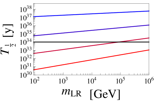
Before closing this discussion on model class (a), we briefly comment on the comparatively low values for the proton lifetime for all cases in which no coloured field is added to the configuration. In the SM (with one Higgs and at 1-loop order) equals at a scale of roughly GeV. Adding a second Higgs, as necessary to complete the bi-doublet in our LR models,99 9 As in the MSSM, where a second Higgs doublet must be present. lowers this GUT scale to roughly GeV. Any addition of a field charged under increases , leading to a further reduction in , unless some coloured field is added at the same time. Thus, all models with a second (or other fields charged under ) but no additional coloured particles will have a GUT scale below GeV. This is indeed quite an important constraint, as is shown in fig. 4. Recall, for a the , while for the . Thus, “colourless” models can have at most one additional , otherwise they are ruled out by proton decay constraints. We note, that the figure is based on a 1-loop calculation and that this conclusion is only strengthened, once 2-loop coefficients are included, compare to the lifetimes quoted in table 1.
III.1.2 Model class [b]: “Fermionic” CKM models
| Configuration | parity? | CKM? | [GeV] | [y] | ||
| 4 | 6 | ☹ | ✓ | |||
| 5 | 11 | ☹ | ✓ | |||
| 5 | 12 | ☹ | ✓ | |||
| 5 | 13 | ✓ | ✓ | |||
| 5 | 7 | ☹ | ✓ | |||
| 5 | 11 | ☹ | ✓ | |||
| 4 | 7 | ☹ | ✓ | |||
| 4 | 7 | ☹ | ✓ | |||
| 4 | 9 | ☹ | ✓ |
We now turn to a discussion of models with additional fermions, see table 2. As discussed in section II, a non-trivial CKM can be generated in LR models with extensions in the fermion sector essentially by three kind of fields, corresponding to vector like copies of the SM fields , and . In the list of 24 different fields shown in table 4 in the appendix, there are in fact several which contain states which can play the role of the VLQs after the breaking of the LR symmetry.
Consider, for example, the case of . The could be generated from , or . Similarly, , or , while , , and . In the SM regime, therefore, different terms from the LR regime can lead to the same effects. We will consider only the three simplest possibilities here, , and , where we have marked the fields with a prime again to note that they have to be introduced in vector-like pairs. Other cases can be constructed in a similar manner. For these three fields the corresponding Lagrangian terms in the LR-regime are:
| (14) | |||||
where and correspond to the SM left and right-handed quarks in the LR regime. Note, that contains the SM-like VEV , while for and the corresponding mass terms are generated from the VEVs of and . Recall that, as discussed in section II, not all terms are necessary and in principle two terms (one mass term and one Yukawa term) are sufficient in all cases to generate the desired structure.
In table 2 we give some simple example models for these cases: , and . Here, we wrote for simply to get a more compact table. Since we count these as two different kinds of fields and at least one or is needed to break the LR symmetry, the minimal seems to be three in these constructions. However, once we impose TeV, no solution with =3 survives, although there are many solutions with =4 and 5. Perhaps the simplest case possible is the model in the first line, which fulfils all our conditions for the price of just two extra and one extra . In general, models which break the LR symmetry via need more copies of fields to get a consistent model with low , . Also, it is possible to conserve parity exactly, as the table shows. However, the model with the smallest that we found still has =13. We have not found any model with less than =7 for the cases and .
In case of models with VLQs, the constraints from proton decay are relatively easy to fulfil, see table 2. This is simply due to the fact that VLQs add a non-zero , by which can be raised to essentially any number desired.
III.2 “Sliding” LR models
We now turn to the discussion of “sliding-LR” models. These are defined as models where the unification is independent of the intermediate scale . In (minimal) supersymmetric extensions of the SM “sliding-LR” models are the only possibility to have a low [24, 27, 28]. However, as we show in this subsection, supersymmetry is not a necessary ingredient to construct sliding models.
We will discuss in the following just two examples of sliding LR models. The first one, based on the idea of “split” supersymmetry [8, 9], shows the relation of our non-supersymmetric sliding models, with the supersymmetric ones discussed in [28]. The second one is based on a SM extension with vector-like quarks, first mentioned in [10] and recently discussed in much more detail in [11]. This second example serves to show, how non-SUSY sliding models can be just as easily constructed as supersymmetric ones.
The sliding conditions can be understood as a set of conditions on the allowed coefficients of the gauge couplings in the LR regime [28], assuring that at 1-loop order at the GUT scale are independent of the additional particle content in the LR regime. In order to achieve successful unification, therefore, it is necessary to first add to the standard model an additional field content at some scale . Although not necessary from a theoretical point of view, we require that is at a “low” scale, i.e. TeV, to ensure that the models predict some interesting collider phenomenology. We will call this additional field content “configuration-X” and “SM+X”. A list of simple X-configurations, which when added to the SM at in the range (few) TeV lead to unification as precise or better than the one obtained in the MSSM, is given in table 6 in the appendix. In this table (at least) one example for each one of our fields is presented.
As the first example, we will discuss the “split SUSY-like” case, which corresponds to . As is well-known, in split SUSY the sparticle spectrum is "split" in two regimes: all scalars (squarks, sleptons and all Higgs fields except ) have masses at a rather high scale, typically GeV, while the fermions, gluino (), wino (), bino () and the higgsinos (, and ) must have TeV-ish masses. This way GCU is maintained with a at the GUT scale as small as is the case in the MSSM (but at a different value of ). However, while in split SUSY is added at the high scale, for our LR constructions we will need this second Higgs at a low scale and, therefore, we call this scenario “split SUSY-like”. Note that, while split SUSY uses fermions at the low scale, GCU can be maintained also with a purely bosonic , since only the 2-loop coefficients change (slightly), which can be compensated by a slight shift in . We note in passing that this particular has, of course, all the interesting phenomenology of split SUSY, like a candidate for the dark matter, or a quasi-stable gluino at the LHC [8].
The quantum numbers of this particular particle content in the LR regime are then: , and , with the coefficients corresponding to this particular given by:
| (15) |
Imposing now the requirement that is independent of the intermediate scale , results in the set of conditions:
| (16) | ||||
| (17) |
Obviously, many different sets of can fulfil these conditions and also realize particle configurations that provide a realistic CKM. To provide just the simplest example, consider scalar CKM models, class [a.1]. These require at least one copy of and each, as discussed in the previous subsection. The simplest sliding solution for this class is given by with (and a GeV). In the LR regime we thus have SM (+ Higgs completed to one bi-doublet) particle content plus . Fig. 5 shows the independence of the GCU from the value of . Note again, that GCU is lost, once is raised above a certain value, the b.f.p. for , including 2-loop coefficients, being TeV.
 |
 |
As in the case of the non-sliding solutions, of course it is also possible to construct sliding-LR models of class [a.2], the simplest 2-field solution is with .
As mentioned above, unification in non-SUSY extensions of the SM have been studied already in [10]. A particular interesting example is the one studied in [11], which adds two kinds of VLQs to the SM particle content, namely and . This model could, potentially, explain the much discussed enhancement in [42, 43]. 1010 10 The latest CMS data now gives much smaller , see the web-page of CMS public results at: twiki.cern.ch/twiki/bin/view/CMSPublic/PhysicsResultsHIG.
As our second sliding-LR example, we thus choose , which in the LR regime corresponds to , with the used to complete the . The coefficients of this configuration are:
| (18) |
The sliding conditions in this case are the same as above and the simplest solution following these conditions and allowing to break the LR symmetry correctly is: , with . The running of the inverse gauge couplings for this example is shown in fig. 6.

IV Uncertainties in new physics scale and proton half-life
One of the aspects of model building for new physics models, rarely discussed in the literature, are uncertainties. While ideally, of course, predictions such as the existence of new particles at the TeV scale should be testable over the whole range of the allowed parameter space, in reality most model builders content themselves with showing that for some particular choice of parameters consistent solutions for their favorite model exist.
In this section we discuss uncertainties for the predictions of our LR models. In these models, once we have fixed the particle content of a particular version, there are essentially three free parameters: , and . However, since there are also three gauge couplings, with values fixed by experiment, for any given model , and are fixed up to some error by the requirement of gauge coupling unification. This results essentially in two predictions: First, the mass scale, where the gauge bosons of the extended gauge sector and (possibly) other particles of the model should show up. This scale coincides, of course, with the range of , as derived from the fit. And, second, derived from and , we obtain a range for the predicted half-life of proton decay.
The analysis of this section uses a minimization, which fits the three measured SM gauge couplings as functions of the three unknowns. We start by discussing the error budget. The total error budget can be divided into a well defined experimental error plus a theory error. For the experimental input we use [44]:
| (19) | |||
The experimental errors quoted are at the 1- confidence level (CL). Note especially the small value of , according to [44], compared to the older value of [45].
Much more difficult to estimate is the theory error. In our discussion presented in section (III) we have used 1-loop -coefficients for simplicity. Two-loop -coefficients for general non-supersymmetric theories, have been derived long ago [46, 47, 47], see also [48], and can be easily included in a numerical analysis. However, a consistent 2-loop calculation requires the inclusion of the 1-loop thresholds from both, light states at the LR-scale and heavy states at the GUT scale. While we do fix in our constructions the particle content in the LR-symmetric phase, we have not specified the Higgs content for the breaking of to the LR group in detail. Thus, the calculation of the GUT scale thresholds is not possible for us, even in principle. The ignorance of the thresholds should therefore be included as (the dominant part of) the theoretical error, once two-loop -coefficients are used in the calculation.
The 1-loop thresholds are formally of the order of a 2-loop effect and, thus, it seems a reasonable guess to estimate their size by a comparison of the results using 1-loop and 2-loop coefficients in the RGE running. This, however, can be done using different assumptions. We have tried the following four different definitions for the theory error:
- •
(i) Perform a search at 1-loop and at 2-loop. Consider the difference as the theoretical error, common to all .
- •
(ii) Perform a search at 1-loop and at 2-loop. Calculate using as the starting point, but keeping the and from the 2-loop calculation. This generates which depend on the group , but does not take into account the overall shift on caused by the change from 1-loop to 2-loop coefficients.
- •
(iii) Perform a search at 1-loop and at 2-loop. Calculate using and as the starting point, but keeping the from the 2-loop calculation. This takes into account both, the shift of and from 1-loop to 2-loop calculation.
- •
(iv) Perform a search at 1-loop. For the b.f.p. of , and found, calculate the values of . Use as the error. One should expect this definition to give, in principle, the most pessimistic error estimate. See, however, the discussion below.
| Def.: | ||||
|---|---|---|---|---|
| (i) | 0.76 | 0.76 | 0.76 | 0.76 |
| (ii) | 0.57 | 0.41 | 1.18 | 0.72 |
| (iii) | 1.31 | 0.34 | 0.40 | 0.68 |
| (iv) | 1.21 | 0.41 | 0.40 | 0.67 |
| Def.: | ||||
|---|---|---|---|---|
| (i) | 0.86 | 0.86 | 0.86 | 0.86 |
| (ii) | 0.46 | 0.46 | 1.18 | 0.70 |
| (iii) | 1.30 | 0.39 | 0.30 | 0.66 |
| (iv) | 1.11 | 0.44 | 0.22 | 0.59 |
Example shifts (“errors”) in determined by the four different methods defined above and for two particular models, discussed in previous sections, are given in table 3. The first and most important observation is that the theory errors estimated in this way are always much larger than the experimental errors on the gauge couplings. We would like to stress, however, that in absolute terms corresponds only to a % shift in the value of , depending on the model. It is found that all four methods lead to very similar , but which of the couplings is assigned the smallest error depends on the method and on the model.


Perhaps more surprising is that method (iv) in the examples shown in the table does not automatically lead to the largest nor to the largest average error, , in these examples 1111 11 For the MSSM method (iv) indeed leads to the largest , see below.. We can attribute this somewhat unexpected result to the correlated shifts induced by the simultaneous change in and in method (iv), which can even conspire in some models to give an unrealistically small deviation in one particular coupling, see the value of in the second model shown in table 3, for example.
In fig. 7 we then show the distributions using the four different set of values of for the model used in the left panel of table 3. Here, the (denoted by the cross) and the corresponding 1, 2- and 3- CL contours are shown in the plane , where is the proton decay half-life estimated via eq. (10). While at first glance, the different methods seem to produce somewhat different results, a closer inspection reveals that the two main conclusions derived from this analysis are in fact independent of the method. First, in all four methods the model is excluded by the lower limit for the proton decay half-live from Super-K [41, 37] data at the one sigma level, but becomes (barely) allowed at 2- CL. And, second, while the model has a preferred value for the scale within the reach of the LHC, the upper limit on - even at only 1- CL! - is very large, between [] GeV depending on the method. The model could therefore be excluded by (a) a slight improvement in the theoretical error bar or (b) from an improved limit on the proton decay, but not by direct accelerator searches. This latter conclusion is, of course, not completely unexpected, since the value of enters in the analysis only logarithmically as the difference between and .
As fig. 7 shows, in three of the four methods the error in the determination of the is around orders of magnitude at one sigma, while in method (ii) - due to the correlation with - we find approximately y. This is mainly due to a change in the GUT scale, when going from the 1-loop to the 2-loop -coefficients. Note, that the value of enters in the fourth power in the calculation of ; thus, an error of a factor of 100 corresponds only to a shift of a factor of in the GUT scale.


In fig. 8 we show the distributions, for the model on the right panel of table 3, using two of the four methods for determining of table 3. The plots for methods (ii) and (iii) lead to results similar to (i) and (iv), respectively, and are therefore not shown. Again, is only very weakly constrained in this analysis, but for this model, the b.f.p. of the GUT scale is much larger, around GeV, so proton decay provides hardly any constraints on this model. Note the strong correlation between and in the plot on the left, which leads to a much larger “error” bar in the predicted range of the proton decay half-life for this model, roughly 5 orders of magnitude at one sigma CL.
We have repeated this exercise for a number of different LR models 1212 12 Among them the two “minimal” LR models discussed in the introduction., see the appendix and discussion in the previous section and have always found numbers of similar magnitude. We have checked, however, that these “large” shifts in are not a particular feature of our LR models. For this check we have calculated also for a number of models with only the SM group up to the GUT scale (see appendix). There, instead of we used the energy where the new particles appear, call it , as a free parameter. Very similar values and variations for are found in this study too. It may be interesting to note that the smallest we found corresponds to a model which is essentially like split supersymmetry 1313 13 This is the first example of SM+X configurations discussed in section III.2. with a of only . (In methods (ii)-(iv) the vary for this model between and with a mean of .) On the other hand, for the MSSM we find a and values of even up to , depending on which of our four methods is used. Thus, the uncertainties discussed in this section should apply to practically all new physics models, which attempt to achieve GCU.


Reducing the theory error on will be possible only, if thresholds are calculated at both new physics scales, and . Since this task is beyond the scope of the present work, in fig. 9 we show plots as a function of the unknown theory error . The model considered is excluded by the proton decay constraint at 2- CL up to an error of roughly , indicating that even a minor improvement in the theory error can have important consequences for all models with a relatively low GUT scale, say GeV. On the other hand, in order to be able to fix the LR-scale to a value low enough such that accelerator tests are possible, requires a much smaller theory error. The exact value of this “minimal” error required depends on the model, but as can be seen from fig. 9 theory errors of the order of will be necessary.
V Conclusions
In this work we attempted to construct a comprehensive list of non-SUSY models with LR-symmetric intermediate stage close to the TeV scale that may be obtained as simple low-energy effective theories within a class of renormalizable non-SUSY SO(10) grand unifications assuming some of the components of scalar representations with dimensions up to 126 to be accidentally light. In order to make our way through the myriads of options we assumed that all such light fields (besides those pushed down by the need to arrange for the low LR breaking scale) necessary to maintain the SO(10)-like gauge coupling unification are clustered around the same (TeV) scale.
Remarkably enough, the vast number of settings that pass all the phenomenological constraints (in particular, the compatibility with the quark and lepton masses and mixings, the current proton lifetime limits, perturbativity and gauge coupling unification) can be grouped into a relatively small number of types characterised, in our classification, by the extra fields underpinning the emergence of the SM flavour structure. Needless to say, the popular low-scale LR alternatives to the MSSM such as, e.g., split-SUSY, simple extensions of the mLR and/or mLR models, are all among these.
In the second part of the study we elaborate in detail on the theoretical uncertainties affecting the possible determination of (not only) the LR scale from the low-energy observables focusing namely on the impact of different definitions of the reflecting the generic incapability of the simplistic bottom-up approach to account for most of the details of the full top-down analysis. To this end, we perform a numerical analysis of a small set of sample scenarios to demonstrate how difficult it is in general to extrapolate the low-energy information over the “desert” to draw any strong conclusion about the viability of the underlying unified theory without a detailed account for, e.g., the GUT-scale thresholds and other such high-scale effects. Nevertheless, within the bottom-up approach employed in this study the character of our results is inevitably just indicative and further improvements are necessary before drawing any far-fetched conclusions. To this end, the simple classification of the basic potentially realistic schemes given in Sect. III may be further improved in several directions, among which perhaps the most straightforward are, e.g., the viability of arranging the considered spectra in specific SO(10) GUTs, their perturbativity beyond the unification scale, etc.
Acknowledgements
This work is supported in part by EU Network grant UNILHC PITN-GA-2009-237920. C.A. and M.H. also acknowledge support from the Spanish MICINN grants FPA2011-22975, MULTIDARK CSD2009-00064 and the Generalitat Valenciana grant Prometeo/2009/091. J. C. R. acknowledges the financial support from grants CFTP-FCT UNIT 777, CERN/FP/123580/2011 and PTDC/FIS/102120/2008. The work of M.M. is supported by the Marie-Curie Career Integration Grant within the 7th European Community Framework Programme FP7-PEOPLE-2011-CIG, contract number PCIG10-GA-2011-303565, by the Research proposal MSM0021620859 of the Ministry of Education, Youth and Sports of the Czech Republic and by the “Neuron” Foundation for scientific research.
Appendix A List of fields
Table (4) gives transformation properties under the group for all representations of up to dimension . For the sake of convenience only, we also give names of certain representations, which have been used in the literature before.
| |||||||||||||||||||||||||||||||||||||||||||||||||||||||||||||||||||||||||||||||||||||||||||||||||||||||||||||||||||||||||||||||||||||
|
Appendix B LR unification: simple configurations
The breaking of the LR symmetry to the : requires the presence of one of the fields: or . All configurations contain then at least one of these fields and also one bi-doublet (to complete “ bi-doublet” basic field content). Table 5 shows the simplest LR configurations for scalar CKM (where the necessary fields are: , , or ) for each one of the fields presented in table 4.
| Extra field | Configuration | |||
|---|---|---|---|---|
Appendix C SM-X extended unification: simple configurations
It is possible to achieve one-step unification of the SM coupling constants withing non-SUSY models. This is performed adding to the SM a new particle content at scale . This particle content can be as simple as the configurations shown in table 6, which added to the lead “” models that unify equal or even better than the MSSM. Therefore, for each one of the fields in table 4 (in the SM version) one of the simplest configurations is obtained as follows: (unification equal or better that the MSSM) and GeV in order to obtain proton life times allowed by the actual bounds.
References
- [1] S. Dimopoulos, S. Raby, and F. Wilczek, Phys.Rev. D24, 1681 (1981).
- [2] L. E. Ibanez and G. G. Ross, Phys.Lett. B105, 439 (1981).
- [3] W. J. Marciano and G. Senjanovic, Phys.Rev. D25, 3092 (1982).
- [4] M. Einhorn and D. Jones, Nucl.Phys. B196, 475 (1982).
- [5] U. Amaldi, W. de Boer, and H. Furstenau, Phys.Lett. B260, 447 (1991).
- [6] P. Langacker and M.-x. Luo, Phys.Rev. D44, 817 (1991).
- [7] J. R. Ellis, S. Kelley, and D. V. Nanopoulos, Phys.Lett. B260, 131 (1991).
- [8] N. Arkani-Hamed and S. Dimopoulos, JHEP 0506, 073 (2005), arXiv:hep-th/0405159.
- [9] G. F. Giudice and A. Romanino, Nucl.Phys. B699, 65 (2004), arXiv:hep-ph/0406088.
- [10] U. Amaldi, W. de Boer, P. H. Frampton, H. Furstenau, and J. T. Liu, Phys.Lett. B281, 374 (1992).
- [11] I. Gogoladze, B. He, and Q. Shafi, Phys.Lett. B690, 495 (2010), arXiv:1004.4217.
- [12] B. Brahmachari, U. Sarkar, and K. Sridhar, Phys.Lett. B297, 105 (1992).
- [13] R. N. Mohapatra, F. E. Paige, and D. P. Sidhu, Phys.Rev. D17, 2462 (1978).
- [14] R. N. Mohapatra and G. Senjanovic, Phys.Rev.Lett. 44, 912 (1980).
- [15] R. N. Mohapatra and G. Senjanovic, Phys.Rev. D23, 165 (1981).
- [16] R. N. Mohapatra and J. W. F. Valle, Phys. Rev. D34, 1642 (1986).
- [17] E. K. Akhmedov, M. Lindner, E. Schnapka, and J. W. F. Valle, Phys.Lett. B368, 270 (1996), arXiv:hep-ph/9507275.
- [18] E. K. Akhmedov, M. Lindner, E. Schnapka, and J. W. F. Valle, Phys. Rev. D53, 2752 (1996), hep-ph/9509255.
- [19] B. Brahmachari, E. Ma, and U. Sarkar, Phys.Rev.Lett. 91, 011801 (2003), arXiv:hep-ph/0301041.
- [20] F. Siringo, Phys.Part.Nucl.Lett. 10, 94 (2013), arXiv:1208.3599.
- [21] C. S. Aulakh, K. Benakli, and G. Senjanovic, Phys.Rev.Lett. 79, 2188 (1997), arXiv:hep-ph/9703434.
- [22] C. S. Aulakh, A. Melfo, A. Rasin, and G. Senjanovic, Phys.Rev. D58, 115007 (1998), arXiv:hep-ph/9712551.
- [23] J. N. Esteves et al., JHEP 1201, 095 (2012), arXiv:1109.6478.
- [24] M. Malinsky, J. C. Romao, and J. W. F. Valle, Phys.Rev.Lett. 95, 161801 (2005), arXiv:hep-ph/0506296.
- [25] S. K. Majee, M. K. Parida, A. Raychaudhuri, and U. Sarkar, Phys.Rev. D75, 075003 (2007), arXiv:hep-ph/0701109.
- [26] P. S. B. Dev and R. N. Mohapatra, Phys.Rev. D81, 013001 (2010), arXiv:0910.3924.
- [27] V. De Romeri, M. Hirsch, and M. Malinsky, Phys.Rev. D84, 053012 (2011), arXiv:1107.3412.
- [28] C. Arbelaez, R. M. Fonseca, M. Hirsch, and J. C. Romao, Phys.Rev. D87, 075010 (2013), arXiv:1301.6085.
- [29] M. Lindner and M. Weiser, Phys.Lett. B383, 405 (1996), arXiv:hep-ph/9605353.
- [30] S. Bertolini, L. Di Luzio, and M. Malinsky, Phys. Rev. D81, 035015 (2010), arXiv:0912.1796 [hep-ph].
- [31] S. Bertolini, L. Di Luzio, and M. Malinsky, Phys.Rev. D87, 085020 (2013), arXiv:1302.3401 [hep-ph].
- [32] X. Calmet, S. D. Hsu, and D. Reeb, Phys.Rev.Lett. 101, 171802 (2008), arXiv:0805.0145 [hep-ph].
- [33] G. Dvali, Fortsch.Phys. 58, 528 (2010), arXiv:0706.2050 [hep-th].
- [34] K. S. Babu and R. N. Mohapatra, Phys.Rev. D86, 035018 (2012), arXiv:arXiv:1203.5544.
- [35] S. Weinberg, Phys. Rev. D22, 1694 (1980).
- [36] H. A. Weldon and A. Zee, Nucl.Phys. B173, 269 (1980).
- [37] Super-Kamiokande Collaboration, K. Abe et al., (2013), arXiv:1305.4391.
- [38] A. J. Buras, J. R. Ellis, M. K. Gaillard, and D. V. Nanopoulos, Nucl.Phys. B135, 66 (1978).
- [39] J. R. Ellis, M. K. Gaillard, and D. V. Nanopoulos, Phys.Lett. B88, 320 (1979).
- [40] F. Wilczek and A. Zee, Phys.Rev.Lett. 43, 1571 (1979).
- [41] Super-Kamiokande, H. Nishino et al., Phys.Rev. D85, 112001 (2012), arXiv:1203.4030.
- [42] ATLAS Collaboration, (2013).
- [43] CMS Collaboration, S. Chatrchyan et al., JHEP 1306, 081 (2013), arXiv:1303.4571.
- [44] Particle Data Group, J. Beringer et al., Phys.Rev. D86, 010001 (2012).
- [45] Particle Data Group, C. Amsler et al., Phys.Lett. B667, 1 (2008).
- [46] D. R. T. Jones, Phys.Rev. D25, 581 (1982).
- [47] M. E. Machacek and M. T. Vaughn, Nucl.Phys. B222, 83 (1983).
- [48] M.-x. Luo, H.-w. Wang, and Y. Xiao, Phys.Rev. D67, 065019 (2003), arXiv:hep-ph/0211440.