Non-Markovian Reduced Systems for Stochastic Partial Differential Equations: The Additive Noise Case

Mickaël D. Chekroun MCDepartment of Mathematics, University of Hawaii at Manoa, Honolulu, HI 96822, USA, and Department of Atmospheric & Oceanic Sciences, University of California, Los Angeles, CA 90095-1565, USA Email address: mdchekroun@math.hawaii.edu Email address: mchekroun@atmos.ucla.edu , Honghu Liu HLDepartment of Atmospheric & Oceanic Sciences, University of California, Los Angeles, CA 90095-1565, USA Email address: hliu@atmos.ucla.edu and Shouhong Wang SWDepartment of Mathematics, Indiana University, Bloomington, IN 47405, USA Email address: showang@indiana.edu, http://www.indiana.edu/~fluid

Abstract.

This article proposes for stochastic partial differential equations (SPDEs) driven by additive noise, a novel approach for the approximate parameterizations of the “small” scales by the “large” ones, along with the derivaton of the corresponding reduced systems. This is accomplished by seeking for stochastic parameterizing manifolds (PMs) introduced in [CLW13] which are random manifolds aiming to provide — in a mean square sense — such approximate parameterizations. Backward-forward systems are designed to give access to such PMs as pullback limits depending through the nonlinear terms on the time-history of the dynamics of the low modes when the latter is simply approximated by its stochastic linear component. It is shown that the corresponding pullback limits can be efficiently determined, leading in turn to an operational procedure for the derivation of non-Markovian reduced systems able to achieve good modeling performances in practice. This is illustrated on a stochastic Burgers-type equation, where it is shown that the corresponding non-Markovian features of these reduced systems play a key role to reach such performances.

Key words and phrases:

Stochastic parameterizing manifolds, non-Markovian reduced equations, Burgers equation driven by additive noise, model reduction, stochastic modeling

2010 Mathematics Subject Classification

34F05, 35B42, 35R60, 37D10, 37L05, 37L10, 37L25, 37L55, 37L65, 60H15

1. Introduction

The reduction problem of stochastic partial differential equations (SPDEs) has attracted a lot of attention recently, and various approaches have been proposed, which include the amplitude equations approach [BM13, PPK+12] and the manifold-based approaches [CLW13, KDKR13] among many others [EMS01, FS09, GKS04, Rob08]; see also the references therein.

In this article, we extend to SPDEs driven by additive noise, the strategy introduced in [CLW13] to derive effective non-Markovian reduced equations. This approach is based on approximate parameterizations of the “small” scales by the “large” ones via the concept of stochastic parameterizing manifolds (PMs), where the latter are random manifolds aiming to improve in mean square error the partial knowledge of the full SPDE solution when compared with its projection onto the resolved modes.

Backward-forward systems are designed to give access to such PMs in practice. The key idea consists here of representing the modes with high wave numbers as a pullback limit depending on the time-history of the modes with low wave numbers. The resulting manifolds obtained by such a procedure are not subject to a spectral gap condition such as encountered in the classical stochastic invariant/inertial manifold theory. Instead, certain PMs can be determined under weaker non-resonance conditions; see (NR) below.

Such an idea of parameterizing the high modes as a functional of the the time-history of the low modes, has been used in the context of 2D-turbulence [EMS01]¹¹ 1 We mention also data-based approaches such as [CKG11, KCRG13] where it has been shown — in the context of climate dynamics — that an appropriate conditioning of the signal’s high-frequency variability on the time-history of the low-frequency modes helps predict the path of the future variations., with the essential difference that the pullback limits considered here are associated with backward-forward systems that are partially coupled in the sense that only the (past values) of the resolved variables force nonlinearly the equations of the unresolved variables, without any feedback in the dynamics of the former; see Eqns. (3.4) below. In such systems, the dynamics of the low modes is simply approximated by its stochastic linear component which helps simplify its integration when compared with the fully coupled versions²² 2 directly rooted in the work of [DPD96]. encountered previously for the approximation of stochastic inertial manifolds [KDKR13], while still making possible the achievement of a good parameterizing quality.

Non-Markovian stochastic reduced systems are then derived based on such a PM approach. The reduced systems take the form of stochastic differential equations (SDEs) involving random coefficients that convey memory effects via the history of the Wiener process, and arise from the nonlinear interactions between the low modes, embedded in the “noise bath.” These random coefficients exhibit typically an exponential decay of correlations whose rate depends explicitly on gaps arising in the non-resonances conditions. It is shown on a stochastic Burgers-type equation, that such PM-based reduced systems can achieve very good performance in reproducing the SPDE dynamics projected onto the resolved modes.

2. Functional framework

Our functional framework takes place in a pair of Hilbert spaces ( $\mathcal{H}_{1}$ , $\mathcal{H}$ ), such that $\mathcal{H}_{1}$ is compactly and densely embedded in $\mathcal{H}$ . Let $A:\mathcal{H}_{1}\rightarrow\mathcal{H}$ be a sectorial operator [Hen81, Def. 1.3.1] such that $-A$ is stable in the sense that its spectrum satisfies $\mathrm{Re}(\sigma(-A))<0$ . To deal with nonlinear SPDEs for which the nonlinear terms are responsible of a loss of regularity compared to the ambient space $\mathcal{H}$ , we consider standard interpolated spaces $\mathcal{H}_{\alpha}$ between $\mathcal{H}_{1}$ and $\mathcal{H}$ (with $\alpha\in[0,1))$ ³³ 3 depending on the problem at hand; see e.g. [Hen81]. along with perturbations of the linear operator $-A$ given by a one-parameter family, $\{B_{\lambda}\}_{\lambda\in\mathbb{R}}$ , of bounded linear operators from $\mathcal{H}_{\alpha}$ to $\mathcal{H}$ , depending continuously on $\lambda$ . Defining $L_{\lambda}$ as $-A+B_{\lambda},$ we are thus left with a one-parameter family of sectorial operators $\{-L_{\lambda}\}_{\lambda\in\mathbb{R}}$ , each of them mapping $\mathcal{H}_{1}$ into $\mathcal{H}$ .

Our main purpose is to present a general strategy⁴⁴ 4 based on the notion of stochastic PMs introduced in [CLW13] in the context of SPDEs driven by linear multiplicative noise. able to provide effective reduced equations for nonlinear stochastic evolution equations driven by additive white noise:

(2.1)

\,\mathrm{d}u=(L_{\lambda}u+F(u))\,\mathrm{d}t+\,\mathrm{d}W_{t};

where $F$ is a continuous nonlinear map from $\mathcal{H}_{\alpha}$ into $\mathcal{H}$ for some $\alpha\in[0,1)$ . For simplicity, we assume $L_{\lambda}$ to be self-adjoint with an orthonormal basis of eigenfunctions $\{e_{k}\}_{k\in\mathbb{N}}$ in $\mathcal{H}$ , with corresponding eigenvalues $\{\beta_{k}(\lambda)\}_{k\in\mathbb{N}}$ . In our setting, only the first $N$ modes will be randomly forced according to

(2.2)

W_{t}(\omega)=\sum_{i=1}^{N}\sigma_{i}W_{t}^{i}(\omega)e_{i},\qquad t\in\mathbb{R},\;\sigma_{i}>0,\;\omega\in\Omega,

where $\{W^{i}\}_{1\leq i\leq N}$ is a family of mutually independent standard two-sided Brownian motions, with paths in $C_{0}(\mathbb{R},\mathbb{R})$ . A natural space of realizations $\Omega=C_{0}(\mathbb{R},\mathbb{R}^{N})$ , can be then associated with $W$ ; $\Omega$ being endowed with its corresponding Borel $\sigma$ -algebra $\mathcal{F}$ , its filtration $\{\mathcal{F}_{t}\}$ , and the Wiener measure $\mathbb{P}$ ; see [Arn98, Appendix A]. Throughout this article we will adopt the formalism of random dynamical systems (RDSs) [Arn98, CLW13, CSG11].

We will assume hereafter that the stochastic evolution equation (2.1) is such that for any initial datum $u_{0}\in H_{\alpha}$ there exists a unique global pathwise solution of (2.1); see e.g. [DPZ08] for conditions.

3. Stochastic Parameterizing Manifolds: Analytic Expressions and “Past-Noise” Dependence

In this section, following [CLW13], stochastic parameterizing manifolds (PMs) are introduced. Backward-forward systems are designed to give access to such PMs in practice. The key idea consists of representing the modes with “high” wave numbers (as parameterized by the sought PM) as a pullback limit depending on the time-history of the modes with “low” wave numbers. The cut between what is “low” and what is “high” is organized as follows. The subspace $\mathcal{H}^{\mathfrak{c}}\subset\mathcal{H}$ defined by,

(3.1)

\displaystyle\mathcal{H}^{\mathfrak{c}}:=\mathrm{span}\{e_{1},\cdots,e_{m}\},

spanned by the $m$ -leading modes will be considered as our subspace associated with the low modes. Its topological complements, $\mathcal{H}^{\mathfrak{s}}$ and $\mathcal{H}^{\mathfrak{s}}_{\alpha}$ in respectively, $\mathcal{H}$ and $\mathcal{H}_{\alpha}$ , will be considered as associated with the high modes. We will use $P_{\mathfrak{c}}$ and $P_{\mathfrak{s}}$ to denote the canonical projectors associated with $\mathcal{H}^{\mathfrak{c}}$ and $\mathcal{H}^{\mathfrak{s}}$ .

3.1. Stochastic parameterizing manifolds: Definition

For a given SPDE of type (2.1), based on [CLW13, Sect. 8], we define a stochastic parameterizing manifold $\mathfrak{M}$ , as the graph of a random function $h^{\mathrm{pm}}$ from $\mathcal{H}^{\mathfrak{c}}$ to $\mathcal{H}^{\mathfrak{s}}_{\alpha}$ which is aimed to provide, for any $u(t,\omega)$ solution of (2.1) given for a realization $\omega$ , an approximate parameterization of the “high” part $u_{\mathfrak{s}}(t,\omega)=P_{\mathfrak{s}}u(t,\omega)$ in terms of the “low” one $u_{\mathfrak{c}}(t,\omega)=P_{\mathfrak{c}}u(t,\omega)$ , so that the mean squared error, $\int_{0}^{T}\bigl\|u_{\mathfrak{s}}(t,\omega)-h^{\mathrm{pm}}(u_{\mathfrak{c}}(t,\omega),\theta_{t}\omega)\bigr\|_{\alpha}^{2}\,\,\mathrm{d}t$ , is smaller than the variance of $u_{\mathfrak{s}}$ , $\int_{0}^{T}\|u_{\mathfrak{s}}(t,\omega)\|_{\alpha}^{2}\;\,\mathrm{d}t$ , whenever $T$ is sufficiently large. In statistical terms, a PM function $h^{\mathrm{pm}}$ is thus such that the fraction of variance of $u_{\mathfrak{s}}(t,\omega)$ unexplained by $h^{\mathrm{pm}}(u_{\mathfrak{c}}(t,\omega),\theta_{t}\omega)$ is less than the unity; see [CLW13, Sect. 8] for more details. More precisely we have

Definition 3.1.

A stochastic manifold $\mathfrak{M}$ given by

\displaystyle\mathfrak{M}(\omega):=\{\xi+h^{\mathrm{pm}}(\xi,\omega)\mid\xi\in\mathcal{H}^{\mathfrak{c}}\},\;\,\omega\in\Omega,

with $h^{\mathrm{pm}}:\mathcal{H}^{\mathfrak{c}}\times\Omega\rightarrow\mathcal{H}^{\mathfrak{s}}_{\alpha}$ being a measurable mapping, is called a stochastic parameterizing manifold (PM) associated with the SPDE (2.1) (for some fixed $\lambda$ ) if the following conditions are satisfied:

(i)

The function $h(\cdot,\omega):\mathcal{H}^{\mathfrak{c}}\rightarrow\mathcal{H}^{\mathfrak{s}}_{\alpha}$ is continuous for each $\omega$ .

(ii)

For any $u_{0}\in\mathcal{H}_{\alpha}$ , there exists a positive random variable $\omega\mapsto T_{0}(\omega;u_{0})$ , such that:

(3.2)

\displaystyle\int_{0}^{T}\!\bigl\|u_{\mathfrak{s}}(t,\omega;u_{0})-h^{\mathrm{pm}}(u_{\mathfrak{c}}(t,\omega;u_{0}),\theta_{t}\omega)\bigr\|_{\alpha}^{2}\,\,\mathrm{d}t<\int_{0}^{T}\!\|u_{\mathfrak{s}}(t,\omega;u_{0})\|_{\alpha}^{2}\,\,\mathrm{d}t,\text{ }\forall\>\omega\in\Omega,\;T>T_{0}(\omega;u_{0}),

where $u_{\mathfrak{c}}(t,\omega;u_{0})=P_{\mathfrak{c}}u(t,\omega;u_{0})$ and $u_{\mathfrak{s}}(t,\omega;u_{0})=P_{\mathfrak{s}}u(t,\omega;u_{0})$ , with $u(t,\omega;u_{0})$ being the solution of the SPDE (2.1) emanating from $u_{0}$ , and driven by the realization $\omega$ .

For a given realization $\omega$ and a given initial datum $u_{0}$ , if $u_{\mathfrak{s}}(\cdot,\omega;u_{0})$ is not identically zero, the parameterization defect of $\mathfrak{M}$ is defined as the following time-dependent ratio:

(3.3)

Q(T,\omega;u_{0}):=\frac{\int_{0}^{T}\bigl\|u_{\mathfrak{s}}(t,\omega;u_{0})-h^{\mathrm{pm}}(u_{\mathfrak{c}}(t,\omega;u_{0}),\theta_{t}\omega)\bigr\|_{\alpha}^{2}\,\,\mathrm{d}t}{\int_{0}^{T}\|u_{\mathfrak{s}}(t,\omega;u_{0})\|_{\alpha}^{2}\,\,\mathrm{d}t},\quad T>T_{0}(\omega;u_{0}).

3.2. Stochastic parameterizing manifolds as pullback limits of backward-forward systems

In this section, we consider the problem of determination of PMs for SPDEs such as given by Eq. (2.1). Theorem 3.1 below provides analytic solutions to this problem, when the nonlinearity $F$ is bilinear, denoted as $B$ below. This is achieved by following the approach introduced in [CLW13] that we adapt to the case of additive noise. In that respect, we consider the following backward-forward system associated with the SPDE (2.1):


(3.4a)	$\displaystyle\mathrm{d}u^{(1)}_{\mathfrak{c}}=L_{\lambda}^{\mathfrak{c}}u^{(1)}_{\mathfrak{c}}\,\mathrm{d}s+\mathrm{d}P_{\mathfrak{c}}W_{s},$	$\displaystyle s\in[-T,0],\quad\;u^{(1)}_{\mathfrak{c}}(s,\omega)\|_{s=0}=\xi,$
(3.4b)	$\displaystyle\mathrm{d}u^{(1)}_{\mathfrak{s}}=\bigl(L_{\lambda}^{\mathfrak{s}}u^{(1)}_{\mathfrak{s}}+P_{\mathfrak{s}}B(u^{(1)}_{\mathfrak{c}}(s-T,\omega))\bigr)\mathrm{d}s+\mathrm{d}P_{\mathfrak{s}}W_{s-T},$	$\displaystyle s\in[0,T],\qquad u^{(1)}_{\mathfrak{s}}(s,\theta_{-T}\omega)\|_{s=0}=0,$

where $L_{\lambda}^{\mathfrak{c}}:=P_{\mathfrak{c}}L_{\lambda}$ , $L_{\lambda}^{\mathfrak{s}}:=P_{\mathfrak{s}}L_{\lambda}$ , and $\xi\in\mathcal{H}^{\mathfrak{c}}$ .

In the system above, the initial value of $u_{\mathfrak{c}}^{(1)}$ is prescribed in fiber $\omega$ , and the initial value of $u_{\mathfrak{s}}^{(1)}$ in fiber $\theta_{-T}\omega$ . The solution of this system is obtained by using a backward-forward integration procedure made possible due to the partial coupling between the equations constituting the system (3.4) where $u^{(1)}_{\mathfrak{c}}$ forces the evolution equation of $u^{(1)}_{\mathfrak{s}}$ but not reciprocally. Note that since, $u_{\mathfrak{c}}^{(1)}$ emanating (backward) from $\xi$ in $\mathcal{H}^{c}$ , forces the equation ruling the evolution of $u_{\mathfrak{s}}^{(1)}$ , the latter depends naturally on $\xi$ and we will emphasize thus this dependence as $u_{\mathfrak{s}}^{(1)}[\xi]$ hereafter. Theorem 3.1 below identifies non-resonance conditions (NR) under which the pullback limit of $u_{\mathfrak{s}}^{(1)}[\xi]$ exists; these non-resonance conditions differing interestingly from those identified for the multiplicative noise case in [CLW13].

As it will be illustrated in the next section in the case of a stochastic Burgers-type equation driven by additive noise, such a pullback limit may be used in practice to give efficiently access to PMs, for a broad class of regimes; see also [CLW13]. The following theorem provides an analytical description of such PMs which in particular emphasizes the dependence on the past of the noise path of these manifolds but of a different form than arising in the multiplicative noise case [CLW13]. As in the latter case though, such features result from the nonlinear self-interactions of the low modes, ‘‘embedded in the noise bath,’’⁵⁵ 5 The nature of this “noise bath” being additive compared to [CLW13]. and such as projected onto the high modes, i.e. from $P_{\mathfrak{s}}B(u^{(1)}_{\mathfrak{c}}(s-T,\omega))$ in (3.4); see the proof sketched below.

Theorem 3.1.

Let us consider the SPDE (2.1) as given within the functional setting of Section 2, with here $F$ assumed to be a bilinear function $B$ . Assume also that $\beta_{n}(\lambda)<0$ for all $n>m$ . Let ${\color[rgb]{0,0,0}\mathcal{I}}:=\{1,\cdots,m\}$ with $m=\textrm{dim}(\mathcal{H}^{\mathfrak{c}})$ . We assume furthermore that the following non-resonance conditions hold:

(NR)			$\displaystyle\text{ }\forall\>\,(i_{1},i_{2})\in\mathcal{I}^{2},\ n>m,\quad\text{ if }\quad\langle B(e_{i_{1}},e_{i_{2}}),e_{n}\rangle\neq 0,\quad\text{ then }\quad\beta_{i_{1}}(\lambda)+\beta_{i_{2}}(\lambda)-\beta_{n}(\lambda)>0,$
			$\displaystyle\text{ }\forall\>\,(i_{1},i_{2})\in\mathcal{I}^{2},\ n>m,\quad\text{ if }\quad\langle B(e_{i_{1}},e_{i_{2}}),e_{n}\rangle\neq 0\text{ and }\sigma_{i_{1}}\neq 0,\quad\text{ then }\quad\beta_{i_{2}}(\lambda)-\beta_{n}(\lambda)>0,$
			$\displaystyle\text{ }\forall\>\,(i_{1},i_{2})\in\mathcal{I}^{2},\ n>m,\quad\text{ if }\quad\langle B(e_{i_{1}},e_{i_{2}}),e_{n}\rangle\neq 0\text{ and }\sigma_{i_{2}}\neq 0,\quad\text{ then }\quad\beta_{i_{1}}(\lambda)-\beta_{n}(\lambda)>0.$

Then the pullback limit of the solution $u_{\mathfrak{s}}^{(1)}[\xi](T,\theta_{-T}\omega;0)$ to (3.4b) exists and is given by:

(3.5)		$\displaystyle h^{(1)}_{\lambda}(\xi,\omega)$	$\displaystyle=\lim_{T\rightarrow+\infty}u_{\mathfrak{s}}^{(1)}[\xi](T,\theta_{-T}\omega;0)$
(3.5)			$\displaystyle=\int_{-\infty}^{0}e^{-\tau L_{\lambda}^{\mathfrak{s}}}L_{\lambda}^{\mathfrak{s}}P_{\mathfrak{s}}W_{\tau}(\omega)\,\mathrm{d}\tau+\int_{-\infty}^{0}e^{-\tau L_{\lambda}^{\mathfrak{s}}}P_{\mathfrak{s}}B(u_{\mathfrak{c}}^{(1)}(\tau,\omega;\xi))\,\mathrm{d}\tau,\quad\text{ }\forall\>\,\xi\in\mathcal{H}^{\mathfrak{c}},\;\omega\in\Omega,$

where $u_{\mathfrak{c}}^{(1)}(s,\omega;\xi)$ is the solution of (3.4a):

(3.6)

u_{\mathfrak{c}}^{(1)}(s,\omega;\xi)=e^{sL_{\lambda}^{\mathfrak{c}}}\xi+P_{\mathfrak{c}}W_{s}(\omega)-\int_{s}^{0}e^{(s-\tau)L_{\lambda}^{\mathfrak{c}}}L_{\lambda}^{\mathfrak{c}}P_{\mathfrak{c}}W_{\tau}(\omega)\,\mathrm{d}\tau.

Moreover, $h^{(1)}_{\lambda}$ has the following analytic expression:

(3.7)		$\displaystyle h^{(1)}_{\lambda}(\xi,\omega)$	$\displaystyle=\sum_{n=m+1}^{N}Z_{n,\lambda}(\omega)e_{n}+\sum_{n=m+1}^{\infty}\sum_{i_{1}=1}^{m}\sum_{i_{2}=1}^{m}\Bigl(A_{\lambda}^{n,i_{1},i_{2}}(\omega)+B_{\lambda}^{n,i_{1},i_{2}}(\omega)\xi_{i_{1}}$
(3.7)			$\displaystyle+C_{\lambda}^{n,i_{1},i_{2}}(\omega)\xi_{i_{2}}+D_{\lambda}^{n,i_{1},i_{2}}\xi_{i_{1}}\xi_{i_{2}}\Bigr)\langle B(e_{i_{1}},e_{i_{2}}),e_{n}\rangle e_{n},$

where $\xi_{i}=\langle\xi,e_{i}\rangle$ , $i=1,\cdots,m$ , and

		$\displaystyle Z_{n,\lambda}(\omega):=\sigma_{n}\beta_{n}(\lambda)\int_{-\infty}^{0}e^{-\tau\beta_{n}(\lambda)}W_{\tau}^{n}(\omega)\,\mathrm{d}\tau,\;\;A_{\lambda}^{n,i_{1},i_{2}}(\omega)=\sum_{j=1}^{4}M_{j,\lambda}^{n,i_{1},i_{2}}(\omega),\;\;B_{\lambda}^{n,i_{1},i_{2}}(\omega)=\sum_{j=5}^{6}M_{j,\lambda}^{n,i_{1},i_{2}}(\omega),$
		$\displaystyle C_{\lambda}^{n,i_{1},i_{2}}(\omega)=\sum_{j=7}^{8}M_{j,\lambda}^{n,i_{1},i_{2}}(\omega),\quad D_{\lambda}^{n,i_{1},i_{2}}:=\int_{-\infty}^{0}e^{(\beta_{i_{1}}(\lambda)+\beta_{i_{2}}(\lambda)-\beta_{n}(\lambda))\tau}\,\mathrm{d}\tau=\frac{1}{\beta_{i_{1}}(\lambda)+\beta_{i_{2}}(\lambda)-\beta_{n}(\lambda)},$

with

	$\displaystyle M_{1,\lambda}^{n,i_{1},i_{2}}(\omega)$	$\displaystyle:=\sigma_{i_{1}}\sigma_{i_{2}}\int_{-\infty}^{0}e^{-\beta_{n}(\lambda)\tau}W_{\tau}^{i_{1}}(\omega)W_{\tau}^{i_{2}}(\omega)\,\mathrm{d}\tau,$
	$\displaystyle M_{2,\lambda}^{n,i_{1},i_{2}}(\omega)$	$\displaystyle:=-\sigma_{i_{1}}\sigma_{i_{2}}\beta_{i_{2}}(\lambda)\int_{-\infty}^{0}\Bigl(e^{-\beta_{n}(\lambda)\tau}W_{\tau}^{i_{1}}(\omega)\int_{\tau}^{0}e^{(\tau-\tau^{\prime})\beta_{i_{2}}(\lambda)}W_{\tau^{\prime}}^{i_{2}}(\omega)\,\mathrm{d}\tau^{\prime}\Bigr)\,\mathrm{d}\tau,$
	$\displaystyle M_{3,\lambda}^{n,i_{1},i_{2}}(\omega)$	$\displaystyle:=-\sigma_{i_{1}}\sigma_{i_{2}}\beta_{i_{1}}(\lambda)\int_{-\infty}^{0}\Bigl(e^{-\beta_{n}(\lambda)\tau}W_{\tau}^{i_{2}}(\omega)\int_{\tau}^{0}e^{(\tau-\tau^{\prime})\beta_{i_{1}}(\lambda)}W_{\tau^{\prime}}^{i_{1}}(\omega)\,\mathrm{d}\tau^{\prime}\Bigr)\,\mathrm{d}\tau,$
	$\displaystyle M_{4,\lambda}^{n,i_{1},i_{2}}(\omega)$	$\displaystyle:=\sigma_{i_{1}}\sigma_{i_{2}}\beta_{i_{1}}(\lambda)\beta_{i_{2}}(\lambda)\int_{-\infty}^{0}\Bigl(e^{-\beta_{n}(\lambda)\tau}\int_{\tau}^{0}e^{(\tau-\tau^{\prime})\beta_{i_{1}}(\lambda)}W_{\tau^{\prime}}^{i_{1}}(\omega)\,\mathrm{d}\tau^{\prime}\int_{\tau}^{0}e^{(\tau-\tau^{\prime})\beta_{i_{2}}(\lambda)}W_{\tau^{\prime}}^{i_{2}}(\omega)\,\mathrm{d}\tau^{\prime}\Bigr)\,\mathrm{d}\tau,$
	$\displaystyle M_{5,\lambda}^{n,i_{1},i_{2}}(\omega)$	$\displaystyle:=\sigma_{i_{2}}\int_{-\infty}^{0}e^{(\beta_{i_{1}}(\lambda)-\beta_{n}(\lambda))\tau}W_{\tau}^{i_{2}}(\omega)\,\mathrm{d}\tau,$
	$\displaystyle M_{6,\lambda}^{n,i_{1},i_{2}}(\omega)$	$\displaystyle:=-\sigma_{i_{2}}\beta_{i_{2}}(\lambda)\int_{-\infty}^{0}\Bigl(e^{(\beta_{i_{1}}(\lambda)-\beta_{n}(\lambda))\tau}\int_{\tau}^{0}e^{(\tau-\tau^{\prime})\beta_{i_{2}}(\lambda)}W_{\tau^{\prime}}^{i_{2}}(\omega)\,\mathrm{d}\tau^{\prime}\Bigr)\,\mathrm{d}\tau,$
	$\displaystyle M_{7,\lambda}^{n,i_{1},i_{2}}(\omega)$	$\displaystyle:=\sigma_{i_{1}}\int_{-\infty}^{0}e^{(\beta_{i_{2}}(\lambda)-\beta_{n}(\lambda))\tau}W_{\tau}^{i_{1}}(\omega)\,\mathrm{d}\tau,$
	$\displaystyle M_{8,\lambda}^{n,i_{1},i_{2}}(\omega)$	$\displaystyle:=-\sigma_{i_{1}}\beta_{i_{1}}(\lambda)\int_{-\infty}^{0}\Bigl(e^{(\beta_{i_{2}}(\lambda)-\beta_{n}(\lambda))\tau}\int_{\tau}^{0}e^{(\tau-\tau^{\prime})\beta_{i_{1}}(\lambda)}W_{\tau^{\prime}}^{i_{1}}(\omega)\,\mathrm{d}\tau^{\prime}\Bigr)\,\mathrm{d}\tau.$

Proof.

(Sketch) First note that the solution of (3.4) can be formally obtained by using the variation-of-constants formula followed by an integration by parts performed to the resulting stochastic convolution terms. By doing so, the solution to (3.4b) is given by $u_{\mathfrak{s}}^{(1)}[\xi](T,\theta_{-T}\omega;0)=-e^{TL_{\lambda}^{\mathfrak{s}}}P_{\mathfrak{s}}W_{-T}(\omega)+\int_{-T}^{0}e^{-\tau L_{\lambda}^{\mathfrak{s}}}L_{\lambda}^{\mathfrak{s}}P_{\mathfrak{s}}W_{\tau}(\omega)\,\mathrm{d}\tau+\int_{-T}^{0}e^{-\tau L_{\lambda}^{\mathfrak{s}}}P_{\mathfrak{s}}B(u_{\mathfrak{c}}^{(1)}(\tau,\omega;\xi))\,\mathrm{d}\tau$ , where $u_{\mathfrak{c}}^{(1)}(\cdot,\omega;\xi)$ is the solution of (3.4a) which takes the form of (3.6).

Since $\beta_{n}(\lambda)<0$ for $n>m$ , the term $e^{TL_{\lambda}^{\mathfrak{s}}}P_{\mathfrak{s}}W_{-T}(\omega)$ converges to zero as $T\rightarrow+\infty$ . This implies that the pullback limit of $u_{\mathfrak{s}}^{(1)}[\xi]$ exists and takes the form given in (3.5) provided that the two integrals involved in the expression of $u_{\mathfrak{s}}^{(1)}[\xi]$ converge as $T\rightarrow+\infty$ . The existence of $\int_{-\infty}^{0}e^{-\tau L_{\lambda}^{\mathfrak{s}}}L_{\lambda}^{\mathfrak{s}}P_{\mathfrak{s}}W_{\tau}(\omega)\,\mathrm{d}\tau$ is a consequence of $\beta_{n}(\lambda)<0$ for $n>m$ . The existence of $\int_{-\infty}^{0}e^{-\tau L_{\lambda}^{\mathfrak{s}}}P_{\mathfrak{s}}B(u_{\mathfrak{c}}^{(1)}(\tau,\omega;\xi))\,\mathrm{d}\tau$ results from the non-resonance condition (NR). This can be seen by expanding the bilinear term $P_{\mathfrak{s}}B(u_{\mathfrak{c}}^{(1)}(\tau,\omega;\xi))$ , using the expression of $u_{\mathfrak{c}}^{(1)}$ given in (3.6), and the fact that $L_{\lambda}$ is self-adjoint. This leads to three types of terms factorized by $\langle B(e_{i_{1}},e_{i_{2}}),e_{n}\rangle e_{n}$ in (3.7): the constant terms, the linear ones and the quadratic ones, where the coefficients $D_{\lambda}^{n,i_{1},i_{2}}$ and $M_{j,\lambda}^{n,i_{1},i_{2}}(\omega)$ therein, are ensured to exist due to the (NR)-conditon. The condition $\beta_{n}(\lambda)<0$ for $n>m$ , ensuring the existence of the Ornstein-Uhlenbeck processes $Z_{n,\lambda}$ , we conclude then to the existence of $h^{(1)}_{\lambda}$ along with its analytic expression given in (3.7).

∎

Note that under similar assumptions to [CLW13, Theorem 8.4], it can be shown furthermore that $h^{(1)}_{\lambda}$ such as provided by the Theorem above, constitutes a PM function for the given SPDE (2.1).

Note also that the random coefficients $Z_{n,\lambda}$ and $M_{j,\lambda}^{n,i_{1},i_{2}}$ given above exhibit decay of correlations as it can be checked by similar calculations performed for the proof of [CLW13, Lemma 9.1]. In particular, $Z_{n,\lambda}$ , $M_{5,\lambda}^{n,i_{1},i_{2}}$ and $M_{7,\lambda}^{n,i_{1},i_{2}}$ are standard Ornstein-Uhlenbeck processes, which exhibit exponential decay of correlations with rates respectively given by $|\beta_{n}(\lambda)|$ , $\beta_{i_{1}}(\lambda)-\beta_{n}(\lambda)$ and $\beta_{i_{2}}(\lambda)-\beta_{n}(\lambda)$ .

As we will illustrate in the next section, the decay of correlations of the aforementioned coefficients are responsible for bringing extrinsic memory effects⁶⁶ 6 in the sense of [Hai09, HO07]. in the $h^{(1)}_{\lambda}$ -based stochastic reduced systems of Eq. (2.1); see (4.2) below. The memory effects will turn out to play an important role in the performance achieved by such systems for the modeling of the SPDE dynamics projected onto the low modes. Unlike with the multiplicative noise case [CLW13], such memory effects come with constant and linear terms which are absent compared to the deterministic case, where the resulting $h^{(1)}_{\lambda}(\xi)$ is reduced to $\sum_{n=m+1}^{\infty}\sum_{i_{1}=1}^{m}\sum_{i_{2}=1}^{m}D_{\lambda}^{n,i_{1},i_{2}}\xi_{i_{1}}\xi_{i_{2}}\big\langle B(e_{i_{1}},e_{i_{2}}),e_{n}\rangle e_{n}.$

4. PM-based Non-Markovian Reduced Systems: Application to a Stochastic Burgers Equation

In this section, we consider the following stochastic initial-boundary value problem on the interval $(0,l)$ :

(4.1)

\mathrm{d}u=\big(\nu u_{xx}+\lambda u-\gamma uu_{x}\big)\mathrm{d}t+\mathrm{d}W_{t}(x,\omega),

supplemented with the Dirichlet boundary conditions, $u(0,t;\omega)=u(l,t;\omega)=0$ , $t\geq 0$ , and initial condition $u(x,0;\omega)=u_{0}(x)$ , $x\in(0,l)$ , where $\nu,\lambda$ and $\gamma$ are positive parameters, and $u_{0}$ is some appropriate initial datum. This problem can be cast into the abstract form (2.1) with $\mathcal{H}:=L^{2}(0,l)$ , and $\mathcal{H}_{1}:=H^{2}(0,l)\cap H_{0}^{1}(0,l)$ , see e.g. [DPDT94]. Here, the noise $W_{t}(x,\omega)$ is taken to be $\sum_{i=1}^{N}\sigma_{i}e_{i}(x)W_{t}^{i}(\omega)$ as above with $e_{i}(x)$ denoting the eigenmodes of the linear part $L_{\lambda}u=\nu u_{xx}+\lambda u$ . Such a stochastic model is inscribed in the long tradition of study of the Burgers turbulence subject to random forces; see among many others [BFK00, Fri95].

Note that the eigenvalues of $L_{\lambda}$ are given by $\beta_{n}(\lambda):=\lambda-\frac{\nu n^{2}\pi^{2}}{l^{2}}$ , $n\in\mathbb{N}$ , and the corresponding eigenvectors are $e_{n}(x):=\sqrt{2/l}\sin(n\pi x/l)$ , $x\in(0,l)$ . We consider below the case where the subspace $\mathcal{H}^{\mathfrak{c}}$ is spanned by the first two eigenmodes, i.e. $\mathcal{H}^{\mathfrak{c}}:=\mathrm{span}\{e_{1},e_{2}\}$ .

By projecting (4.1) against the low modes $e_{1}$ and $e_{2}$ , we have $\mathrm{d}u_{\mathfrak{c}}=\big(L_{\lambda}^{\mathfrak{c}}u_{\mathfrak{c}}+P_{\mathfrak{c}}B(u_{\mathfrak{c}}+u_{\mathfrak{s}})\big)\mathrm{d}t+\mathrm{d}P_{\mathfrak{c}}W_{t}$ , where as before $u_{\mathfrak{c}}:=P_{\mathfrak{c}}u$ with $P_{\mathfrak{c}}$ being the canonical projector associated with $\mathcal{H}^{\mathfrak{c}}$ . By replacing $u_{\mathfrak{s}}(t,\omega):=P_{\mathfrak{s}}u(t,\omega)$ with the pullback limit $h^{(1)}_{\lambda}(\xi,\theta_{t}\omega)$ given by (3.7), we obtain the following reduced equation

(4.2)

\mathrm{d}\xi=\Big(L_{\lambda}^{\mathfrak{c}}\xi+P_{\mathfrak{c}}B\big(\xi+h^{(1)}_{\lambda}(\xi,\theta_{t}\omega)\big)\Big)\mathrm{d}t+\mathrm{d}P_{\mathfrak{c}}W_{t},

aimed to provide an approximation of the SPDE dynamics projected onto the low modes.

Recalling that the random coefficients $Z_{n,\lambda}$ and $M_{j,\lambda}^{n,i_{1},i_{2}}$ contained in the expansion of $h^{(1)}_{\lambda}$ exhibit decay of correlations, we can conclude that extrinsic memory effects in the sense of [Hai09, HO07] are thus conveyed by the drift part of (4.2), making such reduced systems non-Markovian.

The analytic form of $h^{(1)}_{\lambda}(\xi,\omega)$ can be obtained from (3.7) by noting that in this example, the nonlinear interactions $B_{i_{1}i_{2}}^{n}:=\langle B(e_{i_{1}},e_{i_{2}}),e_{n}\rangle$ are given by $B_{i_{1}i_{2}}^{n}=-\gamma\langle e_{i_{1}}(e_{i_{2}})_{x},e_{n}\rangle$ , which take the following form:

(4.3)

B_{i_{1}i_{2}}^{n}=-\frac{\gamma i_{2}\pi}{\sqrt{2}l^{3/2}},\text{ if }n=i_{1}+i_{2};\quad B_{i_{1}i_{2}}^{n}=-\frac{\gamma i_{2}\pi\mathrm{sgn}(i_{1}-i_{2})}{\sqrt{2}l^{3/2}},\text{ if }n=|i_{1}-i_{2}|;\quad B_{i_{1}i_{2}}^{n}=0,\text{ otherwise}.

In particular, for the subspace $\mathcal{H}^{\mathfrak{c}}$ chosen above, we have $\langle e_{i_{1}}(e_{i_{2}})_{x},e_{n}\rangle=0$ for any $n\geq 5$ and $i_{1},i_{2}\in\{1,2\}$ .

From a practical viewpoint, it is however cumbersome to use directly the analytic formula of $h^{(1)}_{\lambda}$ to determine the vector field $P_{\mathfrak{c}}B\big(\xi+h^{(1)}_{\lambda}(\xi,\theta_{t}\omega)\big)$ as $\xi$ varies in $\mathcal{H}^{\mathfrak{c}}$ . Instead, we approximate $h^{(1)}_{\lambda}$ “on the fly” — along a trajectory $\xi(t,\omega)$ of interest — substituting $h^{(1)}_{\lambda}(\xi(t,\omega),\theta_{t}\omega)$ by $u^{(1)}_{\mathfrak{s}}[\xi(t,\omega)](t+T,\theta_{-T}\omega;0)$ as obtained by integration of the backward-forward system (3.4), for $T$ chosen sufficiently large; cf. [CLW13, Sect. 11]. This is much more manageable and leads naturally to consider the following substitutive reduced equation,


(4.4a)		$\displaystyle\mathrm{d}\xi_{t}=\Big(L_{\lambda}^{\mathfrak{c}}\xi_{t}+P_{\mathfrak{c}}B\big(\xi_{t}+u^{(1)}_{\mathfrak{s}}[\xi(t,\omega)](t+T,\theta_{-T}\omega;0)\big)\Big)\mathrm{d}t+\mathrm{d}P_{\mathfrak{c}}W_{t},\quad\xi(0,\omega)=\phi,\quad t>0,$
	where $\phi$ is appropriately chosen according to the SPDE initial datum, and $u^{(1)}_{\mathfrak{s}}[\xi]$ is obtained via
(4.4b)		$\displaystyle\mathrm{d}u^{(1)}_{\mathfrak{c}}=L_{\lambda}^{\mathfrak{c}}u^{(1)}_{\mathfrak{c}}\mathrm{d}s+\mathrm{d}P_{\mathfrak{c}}W_{s},\hskip 130.0002ptu^{(1)}_{\mathfrak{c}}(s,\omega)\|_{s=t}=\xi(t,\omega),\quad s\in[t-T,t],$
(4.4c)		$\displaystyle\mathrm{d}u^{(1)}_{\mathfrak{s}}=\bigl(L_{\lambda}^{\mathfrak{s}}u^{(1)}_{\mathfrak{s}}+P_{\mathfrak{s}}B(u^{(1)}_{\mathfrak{c}}(s-T,\omega))\bigr)\mathrm{d}s+\mathrm{d}P_{\mathfrak{s}}W_{s-T},\hskip 11.99998ptu^{(1)}_{\mathfrak{s}}(s,\theta_{-T}\omega)\|_{s=t}=0,\quad\;s\in[t,T+t],$

which written in coordinate form, gives (cf. [CLW13, Section 11.2]),


(4.5a)			$\displaystyle\,\mathrm{d}\xi_{1}=\Bigl(\beta_{1}(\lambda)\xi_{1}+\frac{\gamma\pi}{\sqrt{2}l^{3/2}}\Bigl(\xi_{1}\xi_{2}+\xi_{2}y_{3}^{(1)}+\sum_{j=3}^{N}y_{j}^{(1)}y_{j+1}^{(1)}\Bigr)\Bigr)\,\mathrm{d}t+\sigma_{1}\,\mathrm{d}W^{1}_{t},\hskip 20.00003ptt>0,$
(4.5b)			$\displaystyle\,\mathrm{d}\xi_{2}=\Bigl(\beta_{2}(\lambda)\xi_{2}+\frac{\sqrt{2}\gamma\pi}{l^{3/2}}\Bigl(-\frac{1}{2}(\xi_{1})^{2}+\xi_{1}y_{3}^{(1)}+\xi_{2}y_{4}^{(1)}+\sum_{j=3}^{N}y_{j}^{(1)}y_{j+2}^{(1)}\Bigr)\Bigr)\,\mathrm{d}t+\sigma_{2}\,\mathrm{d}W^{2}_{t},\hskip 13.00005ptt>0,$
(4.5c)			$\displaystyle\text{with}\hskip 40.00006pt\xi_{1}(0,\omega)=\langle\phi,e_{1}\rangle,\qquad\xi_{2}(0,\omega)=\langle\phi,e_{2}\rangle,$

where $\xi_{t}=\xi_{1}(t,\omega)e_{1}+\xi_{2}(t,\omega)e_{2}$ and $y_{i}^{(1)}$ , $i=3,\cdots,N$ , are obtained via,


(4.6a)		$\displaystyle\,\mathrm{d}y^{(1)}_{1}=\beta_{1}(\lambda)y^{(1)}_{1}\,\mathrm{d}s+\sigma_{1}\,\mathrm{d}W^{1}_{s},\hskip 150.00023pts\in[t-T,t],$
(4.6b)		$\displaystyle\,\mathrm{d}y_{2}^{(1)}=\beta_{2}(\lambda)y_{2}^{(1)}\,\mathrm{d}s+\sigma_{2}\,\mathrm{d}W^{2}_{s},\hskip 150.00023pts\in[t-T,t],$
(4.6c)		$\displaystyle\,\mathrm{d}y_{3}^{(1)}=\Bigl(\beta_{3}(\lambda)y_{3}^{(1)}-\frac{3\gamma\pi}{\sqrt{2}l^{3/2}}y_{1}^{(1)}(s-T,\omega)y_{2}^{(1)}(s-T,\omega)\Bigr)\,\mathrm{d}s+\sigma_{3}\,\mathrm{d}W^{3}_{s-T},\hskip 10.00002pts\in[t,T+t],$
(4.6d)		$\displaystyle\,\mathrm{d}y_{4}^{(1)}=\Bigl(\beta_{4}(\lambda)y_{4}^{(1)}-\frac{\sqrt{2}\gamma\pi}{l^{3/2}}[y_{2}^{(1)}(s-T,\omega)]^{2}\Bigr)\,\mathrm{d}s+\sigma_{4}\,\mathrm{d}W^{4}_{s-T},\hskip 20.00003pts\in[t,T+t],$
(4.6e)		$\displaystyle\,\mathrm{d}y_{j}^{(1)}=\beta_{j}(\lambda)y_{j}^{(1)}\,\mathrm{d}s+\sigma_{j}\,\mathrm{d}W^{j}_{s-T},\hskip 20.00003pts\in[t,T+t],\qquad j=5,\cdots,N,$
	$\displaystyle\text{with}\hskip 10.00002pty^{(1)}_{1}(s,\omega)\|_{s=t}=\xi_{1}(t,\omega),\quad y_{2}^{(1)}(s,\omega)\|_{s=t}=\xi_{2}(t,\omega),\quad y_{i}^{(1)}(s,\theta_{-T}\omega)\|_{s=t}=0,\quad i=3,\cdots,N.$

Numerical results. We assess below the performances achieved by the reduced system (4.5)-(4.6), in the modeling of the pathwise SPDE dynamics on the $\mathcal{H}^{\mathfrak{c}}$ -modes, on one hand; and of the full spatio-temporal field $u$ obtained by direct simulation of the SPDE (4.1), on the other. The importance of the memory terms conveyed by $h^{(1)}_{\lambda}$ is assessed by comparison with the performances achieved by an averaged version of (4.5), which consists of replacing $h^{(1)}_{\lambda}$ in the non-Markovian reduced system (4.2) by its expected value $\mathbb{E}(h^{(1)}_{\lambda})$ :

(4.7)

\mathrm{d}\xi=\Big(L_{\lambda}^{\mathfrak{c}}\xi+P_{\mathfrak{c}}B\big(\xi+\mathbb{E}\big(h^{(1)}_{\lambda}(\xi,\theta_{t}\omega)\big)\big)\Big)\mathrm{d}t+\mathrm{d}P_{\mathfrak{c}}W_{t}.

It can be shown that the concerned random coefficients provided by Theorem 3.1 come each with zero-expectation, resulting in an agreement of $\mathbb{E}(h^{(1)}_{\lambda})$ with the pullback limit associated with the corresponding deterministic backward-forward system. The coordinate form of (4.7) can then be obtained easily; see [CLW13].

For all the simulations below, the noise is taken to be $W_{t}(x,\omega)=\sum_{i=1}^{10}\sigma_{i}e_{i}(x)W_{t}^{i}(\omega)$ , with $\sigma_{1}=\cdots=\sigma_{10}=:\sigma>0$ . The values of $\sigma$ and other system parameters are specified in the captions of the figures given below; the numerical schemes adopted here are those used in [CLW13, Sect. 11] adapted to the additive noise case. In all the numerical experiments that follow, the time step has been taken to be $\delta t=0.01$ , and the mesh size $\delta x$ has been specified as indicated in the Figures captions below.

Figure 1. (a)-(b): The dynamics of the resolved modes modeled by the reduced system (4.5)-(4.6) compared with the SPDE dynamics projected onto the resolved modes; (c)-(d): Analogous results given in (a)-(b) produced by the averaged reduced system (4.7); (e)-(f): Probability density functions (PDFs) of the first two modes amplitudes as estimated from a direct simulation of the SPDE (4.1) (black) vs those such as obtained by simulation of the reduced system (4.5)-(4.6) (red), and its averaged version (4.7) (blue); (g): Time averages of the parameterization defect of

u^{(1)}_{\mathfrak{s}}[\xi]

for various

\lambda

and

\sigma

; here the time average (for a given realization

\omega

) is

\frac{1}{T_{2}-T_{1}}\int_{T_{1}}^{T_{2}}Q(T,\omega;u_{0})\,\,\mathrm{d}T

, where

Q

is computed using (3.3) with

u^{(1)}_{\mathfrak{s}}[u_{\mathfrak{c}}(t,\omega)](t+T,\theta_{-T}\omega;0)

in place of

h^{\mathrm{pm}}_{\lambda}

; and

T_{1}

and

T_{2}

are taken here to be

400

and

1000

, respectively. The vertical dashed line on panel (g) corresponds to

\lambda=1.7\lambda_{c}

which is the value of

\lambda

used for the results shown in panels (a)-(f). Here,

\lambda_{c}:=\nu\pi^{2}/l^{2}

is the critical value at which the leading eigenvalue

\beta_{1}(\lambda)

changes sign. Except in (g), where the values of

\lambda

and

\sigma

are varied, the results reported here were computed for the following values of the parameters:

\gamma=0.5

l=7\pi

\nu=2

\lambda=1.7\lambda_{c}

, and

\sigma=3

. In all cases,

\delta x=0.1679.

Similar to [CLW13], it has been observed that the results reported here are robust w.r.t. the choice of the realization.

Results of Fig. 1 are reported for a regime corresponding to a large amount of noise, and for a domain size $l$ corresponding to small decay rates of correlations of the memory terms⁷⁷ 7 For instance, the decaying rates of $Z_{3,\lambda}$ and $M_{5,\lambda}^{3,1,2}$ are given here by $|\beta_{3}(\lambda)|\approx 0.29$ and $\beta_{1}(\lambda)-\beta_{3}(\lambda)\approx 0.33$ , respectively., so that in particular, such regimes correspond to a natural test bed for assessing the role of the extrinsic memory terms in the modeling performance achieved by the reduced system (4.5)-(4.6). This assessment is accomplished by comparing the results of (4.5)-(4.6) with those of the averaged reduced system (4.7). Figure 1 (a)–(d) shows an episode where (4.5)-(4.6) outperforms (4.7) in modeling the first two modes amplitudes. It has been observed that such episodes repeat very often as time flows, as supported by Fig. 1 (e)-(f) from the estimation of the corresponding probability density functions (PDFs). The latter show that the PDFs of the first two modes amplitudes as simulated by (4.5)-(4.6) coincide almost with those of the SPDE dynamics projected onto the $\mathcal{H}^{\mathfrak{c}}$ -modes, whereas the PDFs simulated from the averaged reduced system (4.7) fails in capturing the correct statistical behavior, demonstrating thus the modeling improvements brought by the non-Markovian features of (4.5)-(4.6).

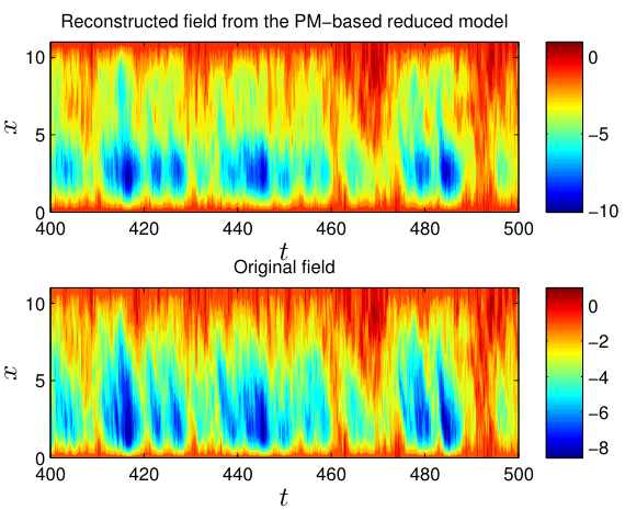
Refer to caption — Figure 2. Spatio-temporal field, $\xi(t,\omega)+u^{(1)}_{\mathfrak{s}}[\xi(t,\omega)](t+T,\theta_{-T}\omega;0)$ , reconstructed from the reduced system (4.5)-(4.6) (upper panel). For comparison the SPDE solution field is plotted in the lower panel. Here the model parameters are $\gamma=0.5$ , $l=3.5\pi$ , $\nu=2$ , $\sigma=1.5$ , and $\lambda=1.7\lambda_{c}$ . Here $\delta x=0.0839.$

It has also been noticed that very good reconstructions of the SPDE solution $u$ can be obtained from the reduced model (4.5)-(4.6), in certain regimes. Figure 2 illustrates such a regime where the coarse-grained features of the spatio-temporal fluctuations of the solution $u$ are well reproduced from the solution $\xi(t,\omega)$ of the reduced model (4.5)-(4.6) once the nonlinear corrective term $u^{(1)}_{\mathfrak{s}}[u_{\mathfrak{c}}(t,\omega)](t+T,\theta_{-T}\omega;0)$ has been added. For all the numerical experiments, the pullback time $T$ in (4.5)-(4.6) is fixed to be $T=2$ . It has been checked that an increase of $T$ has little impact on the quality of the results reported here.

Modeling performances such as reported in Fig. 1 (a)-(d) and Fig. 2, are underpinned by the fact that $h^{(1)}_{\lambda}$ provides a good parameterization of the unresolved modes by the resolved ones as supported by the computations of the (time-averaged) parameterization defects shown in Fig. 1 (g). This is particularly remarkable given that a pathwise SPDE solution $u$ may follow a bimodal behavior such as illustrated in Fig. 3 for the first mode amplitude.⁸⁸ 8 for the same parameters values used for Fig. 2.

Figure 3. (a)-(b) and (c): Bimodal behavior of the SPDE dynamics as projected onto

e_{1}

along with its modeling from the non-Markovian system (4.5)-(4.6) (red), and from its averaged version (4.7) (blue). Noise-induced transitions occurring in time are well-captured by the non-Markovian reduced system when compared to its averaged version. Parameters are those of Fig. 2.

It has been observed that the transitions between the corresponding statistical equilibrium states are very often well captured by the reduced model (4.5)-(4.6) with nevertheless some failures that may occur as time flows; see Fig. 3 (a). The overall bimodal behavior as observed on the first mode is however well-captured by the non-Markovian system (4.5)-(4.6) when compared to its averaged version (4.7) (cf. Fig. 3 (c)), demonstrating once again the importance of the memory effects in reproducing non-trivial statistical features of the dynamics as well as the noise-induced transitions occurring in time; compare Fig. 3 (a) with Fig. 3 (b). The ability of capturing such transitions accurately is tightly related to the modeling problem of the excitation of the small scales by the noise through the nonlinear terms.

The differences in the finer-scale details as observed in Fig. 2 are for instance due to such noise-induced phenomenon and the limited number of modes resolved (here only two). In that respect, it is worthwhile to mention that $u^{(1)}_{\mathfrak{s}}$ obtained by integration of (4.4c), belongs to $\mathrm{span}\{e_{3},\cdots,e_{10}\}$ with its components onto the fifth up to the tenth modes being modeled just as a red noise (see (4.6e)), due to the particular nonlinear self-interactions of the low modes for the problem at hand; see (4.3). Such a “standard” red noise approximation for the fifth to the tenth modes is however not detrimental to the modeling performances achieved by the reduced system (4.5)-(4.6), when these modes do not contain a too important fraction, $\mathfrak{f}_{5}^{10}(T):=|\sum_{j=5}^{10}\langle u,e_{j}\rangle e_{j}|_{L^{2}(0,T;\mathcal{H}_{\alpha})}^{2}|u_{\mathfrak{s}}|_{L^{2}(0,T;\mathcal{H}_{\alpha})}^{-2}$ , of the unresolved variance of the signal, as $T$ evolves. For such a case, the non-Markovian features brought by the more elaborated stochastic “reddish” processes $M_{j,\lambda}^{n,i_{1},i_{2}}$ ( $n\in\{3,4\}$ , $i_{1},i_{2}\in\{1,2\}$ ) — arising typically with non-Gaussian statistics (cf. [CLW13, Fig. 1]) — in the reduced system (4.5)-(4.6), are sufficient to achieve a good parameterization of the excitation of the small scales by the noise, leading to the successes reported in Figures 1, 2 and 3.

When $\mathfrak{f}_{5}^{10}$ happens to get large, the episodes of time where the modeling performances achieved by (4.5)-(4.6) get deteriorated, become more numerous. A remedy to such episodes of deterioration relies on the usage of other parameterizing manifolds based on multilayer backward-forward systems such as introduced in [CLW13]. The latter convey a “matriochka” of nonlinear self-interactions of the low modes which arise typically with a hierarchy of memory effects of more elaborated structures than conveyed by $h^{(1)}_{\lambda}$ ; see [CLW13, Section 11.3] for the multiplicative noise case. The corresponding results for the additive noise case will be reported elsewhere.

Acknowledgments

MDC and HL are supported by the National Science Foundation grant DMS-1049114 and Office of Naval Research grant N00014-12-1-0911. SW is supported in part by National Science Foundation grants DMS-1211218, and DMS-1049114, and by Office of Naval Research grant N00014-11-1-0404.

References

[Arn98] L. Arnold, Random Dynamical Systems, Springer, 1998.
[BFK00] J. Bec, U. Frisch, and K. Khanin, Kicked Burgers turbulence, J. Fluid Mech. 416 (2000), 239–267.
[BM13] D. Blömker and W. W. Mohammed, Amplitude equations for SPDEs with cubic nonlinearities, Stochastics: An International Journal of Probability and Stochastic Processes 85 (2013), no. 2, 181–215.
[CKG11] M. D. Chekroun, D. Kondrashov, and M. Ghil, Predicting stochastic systems by noise sampling, and application to the El Niño-Southern Oscillation, Proceedings of the National Academy of Sciences 108 (2011), no. 29, 11766–11771.
[CLW13] M. D. Chekroun, H. Liu, and S. Wang, On stochastic parameterizing manifolds: Pullback characterization and non-Markovian reduced equations, Preprint, http://arxiv.org/pdf/1310.3896v1.pdf (2013).
[CSG11] M. D. Chekroun, E. Simonnet, and M. Ghil, Stochastic climate dynamics: Random attractors and time-dependent invariant measures, Physica D 240 (2011), no. 21, 1685–1700.
[DPD96] G. Da Prato and A. Debussche, Construction of stochastic inertial manifolds using backward integration, Stochastics Stochastics Rep. 59 (1996), no. 3-4, 305–324.
[DPDT94] G. Da Prato, A. Debussche, and R. Temam, Stochastic Burgers’ equation, Nonlinear Differential Equations Appl. 1 (1994), no. 4, 389–402.
[DPZ08] G. Da Prato and J. Zabczyk, Stochastic Equations in Infinite Dimensions, Encyclopedia of Mathematics and its Applications, vol. 44, Cambridge University Press, Cambridge, 2008.
[EMS01] W. E, J. C. Mattingly, and Y. Sinai, Gibbsian dynamics and ergodicity for the stochastically forced Navier–Stokes equation, Comm. Math. Phys. 224 (2001), no. 1, 83–106.
[Fri95] U. Frisch, Turbulence: The legacy of A. N. Kolmogorov, Cambridge University Press, Cambridge, 1995.
[FS09] E. Forgoston and I. B. Schwartz, Escape rates in a stochastic environment with multiple scales, SIAM J. Applied Dynamical Systems 8 (2009), no. 3, 1190–1217.
[GKS04] D. Givon, R. Kupferman, and A. Stuart, Extracting macroscopic dynamics: model problems and algorithms, Nonlinearity 17 (2004), no. 6, R55–R127.
[Hai09] M. Hairer, Ergodic properties of a class of non-Markovian processes, Trends in stochastic analysis, London Math. Soc. Lecture Note Ser., vol. 353, Cambridge Univ. Press, 2009, pp. 65–98.
[Hen81] D. Henry, Geometric Theory of Semilinear Parabolic Equations, Lecture Notes in Mathematics, vol. 840, Springer-Verlag, Berlin, 1981.
[HO07] M. Hairer and A. Ohashi, Ergodic theory for SDEs with extrinsic memory, Ann. Probab. (2007), 1950–1977.
[KCRG13] D. Kondrashov, M.D. Chekroun, A.W. Robertson, and M. Ghil, Low-order stochastic model and “past-noise forecasting” of the Madden–Julian oscillation, Geophysical Research Letters 40 (2013), no. 19, 5305––5310.
[KDKR13] X. Kan, J. Duan, I. G. Kevrekidis, and A. J. Roberts, Simulating stochastic inertial manifolds by a backward-forward approach, SIAM J. Appl. Dyn. Syst. 12 (2013), no. 1, 487–514.
[PPK⁺12] M. Pradas, G. A. Pavliotis, S. Kalliadasis, D. T. Papageorgiou, and D. Tseluiko, Additive noise effects in active nonlinear spatially extended systems, European J. Appl. Math. 23 (2012), no. 5, 563–591.
[Rob08] A. J. Roberts, Normal form transforms separate slow and fast modes in stochastic dynamical systems, Physica A 387 (2008), 12–38.