Monotone homotopies and contracting discs on Riemannian surfaces
Abstract
We prove a “gluing” theorem for monotone homotopies; a monotone homotopy is a homotopy through simple contractible closed curves which themselves are pairwise disjoint. We show that two monotone homotopies which have appropriate overlap can be replaced by a single monotone homotopy. The ideas used to prove this theorem are used in [CL2] to prove an analogous result for cycles, which forms a critical step in their proof of the existence of minimal surfaces in complete non-compact manifolds of finite volume.
We also show that, if monotone homotopies exist, then fixed point contractions through short curves exist. In particular, suppose that is a simple closed curve of a Riemannian surface, and that there exists a monotone contraction which covers a disc which bounds consisting of curves of length . If and , then there exists a homotopy that contracts to over loops that are based at and have length bounded by , where is the diameter of the surface. If the surface is a disc, and if is the boundary of this disc, then this bound can be improved to .
Introduction.
The central object of study is a monotone homotopy on a Riemannian surface . A monotone homotopy is one in which every curve is simple, and in which pairs of curves do not self-intersect. For the purposes of this article, we will assume that all curves are contractible. If the manifold is a -disc, then this can be rephrased as follows.
Definition 0.1
Let be a Riemannian manifold with boundary diffeomorphic to that of the -disc. Let be a smooth map such that , , and is a simple closed curve parametrized by for each . We will say that is a weakly monotone homotopy if closed -discs bounded by satisfy the inclusion for every and with . If these discs satisfy a stronger condition that , where is the interior of , then the homotopy will be called strictly monotone, or just monotone.
Figure 1(a) depicts a strictly monotone homotopy of to the point , while Figure 1(b) depicts a homotopy that is not monotone. This definition can be trivially extended to homotopies connecting a simple closed contractible curve to a point on any closed Riemannian surface not diffeomorphic to the -disc. There is one technicality, however; if is diffeomorphic to , then there is an ambiguity due to non-uniqueness of . We agree to resolve it by allowing any possible choice of the system of discs that is continuously dependent on , and that has the monotonicity (or strict monotonicity) property.
There are several natural conjectures concerning the existence of monotone homotopies in the presence of regular homotopies. The first one of these conjectures concerns contractions of a disc, and the second concerns contractions of a simple closed curve on a Riemannian surface.
Conjecture 0.2
Suppose that is a Riemannian manifold which is diffeomorphic to a disc. If there is a contraction of through curves of length at most then, for every , there is a monotone contraction of through curves of length at most .
Conjecture 0.3
Suppose that is a Riemannian surface and that is a simple closed curve on . If is contractible through curves of length at most then, for every , there is a monotone contraction of a simple closed curve through curves of length at most which covers .
In the second conjecture, when we say that the monotone contraction covers , we mean that is contained in the the disc with boundary which is the image of the contraction.
Both of these conjectures can be simplified by using the following theorem of independent interest proved by the first author and Yevgeny Liokumovich in [CL1]:
Theorem 0.4
(G. R. Chambers, Y. Liokumovich [CL1]) Let be a Riemannian surface. Let be a closed curve in . Suppose there exists a homotopy such that ; , and the length of is at most for all . Then, for any , there exists a homotopy , such that ; ; the length of is at most , and is a simple closed curve for every .
By applying this theorem, Conjectures 0.2 and 0.3 can be reduced to statements about homotopies through simple closed curves.
Our main theorem is a “gluing” statement about monotone homotopies. A monotone homotopy from an initial curve to a final curve traverses an annulus with as its “outer” boundary component, and as its “inner” boundary component. We begin by stating the relationship between the two annuli formed by the two homotopies which we are going to glue together:
Definition 0.5
Suppose that and are two monotone homotopies with initial curves and , and with final curves and . Suppose further that two continuous of families of discs have been chosen that have boundaries equal to the curves of and of , respectively. For every curve of or , we use to denote the disc that fills . In particular, the curves are simple and bound discs for and . We will say that and are nested if . Furthermore, we will say that and are strictly nested if
- 1.
- 2.
- 3.
To state our theorem we also require the following definition:
Definition 0.6
Let and be two closed curves in a Riemannian manifold .
We will say that and satisfy the simple intersection property if, for every two points of intersection of and , they are consecutive on if and only if they are consecutive on .
We can now state our main gluing theorem.
Theorem 0.7
Suppose that and are monotone homotopies which are nested, and which pass through curves of length at most . Furthermore, suppose that there is a closed curve such that, using the notation from Definition 0.5,
- 1.
lies in the closed annulus .
- 2.
minimizes length among all closed curves in this annulus homotopic to .
- 3.
and satisfy the simple intersection property, and and also satisfy the simple intersection property.
Then, for every , there exists a monotone homotopy with a corresponding family of discs such that the disc which fills the initial curve contains , and the disc which fills the final curve is contained in . Additionally, we can construct so that it is composed of curves of length at most .
Suppose that and are strictly nested, and that both pass through curves of length at most . Then, for every , we can find a monotone homotopy composed of curves of length at most , which begins on , and which ends on .
This suggests a natural way to approach Conjectures 0.2 and 0.3. First, we apply Theorem 0.4 to reduce the problem to the case where the homotopies pass through simple closed curves. Next, we choose a finite sequence of simple closed curves from this homotopy. We then produce a sequence of monotone homotopies such that is strictly nested with respect to for all , and such that is contained in the annulus which traverses. The idea of how to produce this sequence is to choose and close together, and then to perturb each within its normal neighborhood. We then apply Theorem 0.7 to the pair and obtaining a new homotopy which covers both and , and which is strictly nested with respect to . We then iterate this process for the new homotopy and , obtaining a homotopy which covers , and , and which is strictly nested with respect to . Continuing this process for all of the homotopies we achieve the desired result.
This procedure fails because the perturbation argument does not yield a sequence of strictly nested homotopies. Instead, we can attempt to execute this approach for nested homotopies. In this case, the perturbation argument produces a sequence of nested homotopies, but the proof still fails due to the fact that the inductive step no longer holds. In particular, if , , and form a sequence of nested homotopies, and if we attempted to glue together and as per Theorem 0.7, then the result may no longer be nested with respect to .
In [CL2], the first author and Y. Liokumovich use exactly this technique (and a proof which mimics the proof of Theorem 0.7) to solve conjectures analogous to Conjecture 0.2 and 0.3 for one parameter families of sufficiently regular cycles. This result plays a crucial role in their proof that every complete manifold of finite volume contains a (possibly non-compact) minimal surface.
0.1 Contracting discs in Riemannian manifolds
Conjectures 0.2 and 0.3, if true, have numerous implications. One which we are particularly interested in is the following. Assume that is a smooth surface, possibly with boundary, and that is a simple closed curve on . Assume that can be contracted to a point via free loops (closed curves) of length at most . We would like to contract over closed curves based at a point so that the maximal length of these curves is as small as possible. Can we estimate the required maximal length in terms of and the diameter of ? Such a result would have a large number of applications, some of which will be discussed at the end of the introduction. This problem is already interesting when is a -disc endowed with a Riemannian metric and is its boundary. The simple example of a Riemannian metric on that looks like a long thin finger shown in Figure 2 demonstrates that we cannot estimate the required length in terms of alone, and this example suggests that at the very least we need to add a summand equal to . In this example, we can contract the boundary of the disc via short closed curves to a point far from (see Figure 2(a)). To replace this homotopy by one composed of loops based at a point , we connect and by a minimizing geodesic . In the course of our new homotopy, we travel along to one of the closed curves in the original homotopy, travel along this curve, and then return back along (Figure 2(b)). At some moment we end up at a loop that consists of two copies of traversed in opposite directions. This loop can then be contracted to along itself.
Of course, there are other, more complicated Riemannian metrics on the -disc, such as the metric depicted in Figure 3. There is also the family of Riemannian metrics considered in [FK]. For these metrics, the connection between the length of curves in the “best” free loop homotopy and the length of curves in the “best” fixed point homotopy is not so evident.
Our first theorem asserts that if Conjecture 0.2 is true, then adding the summand and an arbitrarily small to will always suffice. It is quite possible that one does not need , but this does not seem to follow from a compactness argument, as when , our homotopies can become wigglier and wigglier. (More formally, we do not establish a bound on the Lipschitz constants of our homotopies as .)
Theorem 0.8
Let be a Riemannian manifold with boundary diffeomorphic to the standard disc of dimension . Denote its diameter by . Suppose there exists a homotopy connecting the boundary of to some point such that the length of every closed curve in this homotopy does not exceed a real number . If Conjecture 0.2 is true then, for any and for any , there exists a fixed point homotopy that connects with , and passes through loops that are based at and have length not exceeding .
In particular, if there exists a monotone contraction of through curves of length at most , then the result holds.
Proof. By Conjecture 0.2, there exists a strictly monotone homotopy between and over simple curves of length at most . Fix a point on , and let be a minimal geodesic connecting to . The length of is at most . For each , there is exactly one such that the curve goes through . Let this curve be denoted by . Note that, if intersects a curve in multiple times, then we will be able to find multiple values for that result in the same curve.
Our new contraction of through curves based at is now defined as follows. For each , define to be the curve
where is the segment of traversed from to . Each curve in this homotopy is bounded in length by . Furthermore, it ends at , which can obviously be contracted to through curves based at of length no more than . This completes the proof.
Our second theorem deals with the general case of a simple contractible curve on a surface endowed with a Riemannian metric.
Theorem 0.9
Let be a closed Riemannian surface of diameter . Let be a simple closed curve in , and a point on . If there exists a homotopy between and a point that passes through closed curves of length not exceeding , and if Conjecture 0.3 is true, then there exists a homotopy that contracts to through loops that are based at and have length .
In particular, if there is a monotone contraction of a simple closed curve through curves of length at most which covers , then the result holds.
The proof of this theorem is significantly more involved; we will postpone its proof until the end of the article.
The questions considered in this paper fall within the realm of questions of investigating geometric properties of “optimal” homotopies.
Another example of such a question was a long-standing question of S. Frankel and M. Katz posed at the end of their paper [FK]. They asked if one contract the boundary of a Riemannian -disc so that the length of curves in the homotopy is majorized above in terms of the diameter , area , and the length of the boundary of the manifold? Note that this question is a modification of an earlier question asked by M. Gromov ([Gr], p. 100). The positive answer to this question was given by Y. Liokumovich, A. Nabutovsky and the second author of this paper in [LNR]. In particular, it was shown that can be contracted over curves of length at most , where is the length of . This estimate is optimal up to a multiplicative factor in the second term. When , [LNR] provides a better bound of . This was improved to the asymptotically tight upper bound by P. Papasoglu in a recent paper [P]. Note that it is impossible to bound the length of curves in the best homotopy solely in terms of the area of , as an example of a three-legged star fish with long tentacles depicted in Figure 4 demonstrates. It is also impossible to bound the length solely in terms of the diameter of , as was proved by Frankel and Katz in [FK], answering the original version of the question of M. Gromov mentioned above.
A closely related family of questions deals with establishing the existence of various upper bounds on the maximal length of optimal sweep-outs and slicings of surfaces either by closed curves or, more generally, by cycles. For example, it was shown by Y. Liokumovich that there does not exist a universal diameter bound for the maximal length of curves or cycles in an optimal sweep-out of a closed Riemannian surface (see [L1] and [L2]). On the other hand, F. Balacheff and S. Sabourau have found an upper bound for the maximal length of a cycle in an optimal sweep-out of a surface in terms of the genus and the area of the surface (see [BS]). Also, a “short” sweep-out of a Riemannian -sphere is possible if one assumes that there is no “short” geodesics of index . This follows from the results of C. B. Croke in [C]. In this case, the maximal length of a cycle can be bounded by the area or the diameter of the surface.
Note that we cannot hope to prove Conjecture 0.2 when one has a simple curve on a surface, or even a simple closed curve in a disc that is not assumed to be the boundary of that disc. This fact makes proving Theorem 0.9 more difficult than Theorem 0.1, and is the reason for the appearance of the extra in our upper bound. We are grateful to Yevgeny Liokumovich for first attracting our attention to this fact in conjunction with the example shown in Figure 5. This figure depicts a metric on a Riemannian -disc and a curve such that the optimal homotopy contracting the curve to a point is not monotone. Notice that there are three bumps depicted in this figure: two of them are long and thin and the one in the middle is short and asymmetric. It takes less length to go under the middle bump than over it. The original curve winds around the two thin bumps, and goes over the short one. In order to contract to a point, it has to be stretched over the thin bumps but, because they are long, the length of the curve will necessarily increase in the process. Thus, to begin with, it makes sense to first homotope to , which runs below the middle bump. is shorter than , so we can “spend” this “excess” length on dragging the curve over the two thin bumps one at a time. This corresponds to the curves and in Figure 5. We now have to push the curve over the middle bump. This homotopy results in , which can then be easily contracted to a point. The resulting homotopy is not monotone. Note that is not the boundary of the disc, and so this example does not constitute a counterexample to Conjecture 0.2.
Applications. If Conjectures 0.2 and 0.3 are true, then Theorem 0.8 and Theorem 0.9 will have have numerous immediate and potential applications to the geometry of loop spaces of Riemannian -spheres, to questions about the lengths of geodesics, and to problems about optimal sweep-outs.
In particular, Theorem 0.9 provides a canonical way of obtaining a “short” based loop homotopy out of a “short” free loop homotopy on a Riemannian surface. The second author has encountered this problem many times, and each time it was solved using ad hoc methods. Specifically, Theorems 0.8 and 0.9 can be applied in the following situations.
(1) Lengths of geodesics on Riemannian -spheres.
Let be an arbitrary pair of points on a Riemannian -sphere of diameter . A. Nabutovsky together with the second author have demonstrated that there exist at least geodesics joining them of length at most (see [NR2]). If , then this bound becomes (see [NR1]). We have noticed that applying Theorem 0.9 dramatically decreases the complexity of proofs in [NR1] and [NR2], and improves the bounds in [NR2] to , and the bounds in [NR1] to . These improvements are due to the fact that the main technical difficulty encountered in [NR1] and especially in [NR2] is the possible formation of intersections between various closed curves in a homotopy between a closed curve and a point.
(2) Geometry of the loop spaces of Riemannian -spheres. Applying Theorem 0.9 will immediately generalize Theorem 1.1 in [NR3] to the free loop space of a Riemannian -sphere . To be more precise, one can show that any map , where is a free loop space on , is homotopic to a map that passes through curves of length that do not exceed . Here, is the diameter of , is the number of distinct non-trivial periodic geodesics on of length at most , and is a function of that can be written down explicitly. Moreover, one can explicitly majorize the lengths of loops in an “optimal” homotopy connecting and in terms of and .
1 Proof of Theorem 0.7
In this section we prove Theorem 0.7, which we recall below:
Theorem 1
Suppose that and are monotone homotopies which are nested, and which pass through curves of length at most . Furthermore, suppose that there is a closed curve such that, using the notation from Definition 0.5,
- 1.
lies in the closed annulus .
- 2.
minimizes length among all closed curves in this annulus homotopic to .
- 3.
and satisfy the simple intersection property, and and also satisfy the simple intersection property.
Then, for every , there exists a monotone homotopy with a corresponding family of discs such that the disc which fills the initial curve contains , and the disc which fills the final curve is contained in . Additionally, we can construct so that it is composed of curves of length at most .
Suppose that and are strictly nested, and that both pass through curves of length at most . Then, for every , we can find a monotone homotopy composed of curves of length at most , which begins on , and which ends on .
Proof. Without loss of generality, let us assume that the homotopies and are strictly monotone and pass through smooth curves. Let be the disc corresponding to the final curve of , and let be the disc corresponding to the initial curve of . We may also assume that and are disjoint. If necessary, all of these properties can be achieved by an arbitrarily small perturbation of and .
Let us consider the closure of the annulus . Let be the shortest closed curve among all closed curves in this closed annulus that are homotopic to . By hypothesis, we may assume that and the final curve of have the simple intersection property, and that and the initial curve of also have the simple intersection property. Note that the length of is at most . It is easy to see that is a simple closed curve. Let be a closed domain diffeomorphic to the -disc that has as its boundary and is contained in . We may assume that the initial and final curves in and are transverse to up to a small perturbation.
We will form as follows. We will define a process which transforms into a weakly monotone homotopy which starts at the boundary of a disc which contains , and which ends at , which transforms into a weakly monotone homotopy which starts at and ends on the boundary of a disc contained in . This process will increase the lengths of curves by at most . will then will then be defined as the concatenation of the modified and perturbed slightly so that it is strictly monotone.
We will define this process in three steps. Step 1 defines the above process for modifying , Step 2 defines the above process for modifying , and Step 3 defines the concatenation of the two homotopies.
In all of these steps, the homotopies formed may not be strictly monotone, and may contain curves with tangential self-intersections (or segments which agree). These will be resolved in the final step by a slight perturbation. Throughout this section, we will use the notation to denote the disc that has boundary equal to the curve , and we will use the notation to denote the disc that has boundary .
Step 1. We will modify the homotopy to obtain a new homotopy so that the new homotopy will be monotone, will be outside of the disc bounded by , and .
First, we will construct a -parameter family of simple closed curves that can possibly have a finite number of discontinuities (as a function of the parameter ). We will then remove the discontinuities.
The new curves will be constructed as follows. The general principle is to “push” (arcs of) outside of the interior of the disc . More specifically, if as in Figure 6(a), then we will let . If or as in Figure 6(b), then we will let .
Now suppose that and that neither one is a subset of the other. Let us consider , a subdivision of such that and otherwise.
Let us consider those arcs of that are inside . Clearly those arcs will be inside as well. However, also, by the monotonicity of the homotopy , these arcs will be outside of . Thus, they will lie in the closed annulus , the closure of .
Consider one such arc of between and . These two points coincide with points and which subdivide the curve into two arcs. Let us select the arc of between these two points which is path homotopic to the arc of with the same endpoints which lies inside the closed annulus between and . Now replace this arc of by . The resulting curve will not be contractible in the closed annulus between and . Also, the length of does not exceed the length of the arc of that it replaced, as otherwise would not be the shortest non-contractible curve in the closed annulus. Therefore, the resulting curve will have length bounded by the length of the original curve. Note that is outside of since and satisfy the simple intersection property, and so (arcs of) curves in the homotopy can move only outside. Furthermore, if and are strictly nested, then and do not intersect, and so . Also, by the hypotheses of lemma, . As a result, .
Additionally, note that the resulting map regarded as a -parametric family of closed curves depending on the parameter is monotone, but its dependence on is not necessarily continuous.
The possible discontinuities may only occur at those curves that are tangent to at some points. (Here it is convenient for us to think that is smooth. While, in general, will be only piecewise smooth, we can perturb it into an arbitrarily close smooth curve of arbitrarily close length. This replacement of by a very close smooth curve adds a summand to our estimates that can be made arbitrarily small. Therefore, without loss of generality we can assume that is smooth.) Without loss of generality, we can also assume that, for each value of , there is at most one point where and are tangent, and that all of these tangencies are non-degenerate. (If not, we can perturb so that the resulting homotopy has these properties, and so that the curves increase in length only by an arbitrarily small amount.) Let us modify the family so that the singularities at tangential points are resolved.
In order to do this, let us consider such that the curve is tangent to at the point . Let us consider the following two cases:
Case A. The set of intersections of with the curve consists of the one point . First, consider the situation in which as in Figure 7(a), where denotes the interior of the set. This situation is not possible since the homotopy is monotone, and since . Hence, there are two possibilities: the curve , as in Figure 7(b), or , as in Figure 7(c). In the former case, we let , and in the latter case, we let .
In both of these cases, the problem with continuity of the newly constructed -parametric family of curves at cannot arise. Indeed, let us consider the first case, when as in Figures 7(a) and 8(b). The second situation will be analogous. Let us consider a family of curves . We can choose to be small enough so that there are no points where and are tangent for any in the interval . By the monotonicity of the homotopy , if , so for each , as depicted in Figures 8(b) and 8(c). Since , is continuous at from the right. For the other direction, each curve with has exactly two points of intersection with that we will denote and , where . Note that and , where by the monotonicity of the homotopy , and both and vary continuously with as approaches from the left, and approach and , respectively. Note that the segment is inside of . Hence, our algorithm continuously replaces this segment by the segment . Thus, we obtain continuity from the left, as shown in Figure 8(d).
Case B. Let us now assume that intersects at points for some . Let be a partition of the unit interval such that , and where all the intersections are transverse except for , where it touches the curve at .
Let us consider the arcs and . There are two possibilities to consider: either both and lie inside , or both of them lie outside. It is not possible for one of the arcs to be inside, and for the other to be outside, because that would imply that either the intersection at is transverse, or the tangency at this point is degenerate, and either of these options contradicts our assumptions.
First, assume that both arcs and are outside of . Then, according to our algorithm, the arcs of the new curve on the interval will remain unchanged. Let us consider , where is selected so that the curves in the family do not have any additional tangential intersections, as in Figures 9(a) and 9(b). Then, for any nearby curve, the corresponding arc is either outside , or has two more additional transverse intersections with in small neighbourhood of . Let us denote these intersections as and . Thus, will locally be formed by continuously replacing by an arc of between the same endpoints. Hence, in this case, changes continuously when is near . Note that while and can come in any order as is indicated in Figure 9, this fact does not affect the above analysis.
Thus, the only problematic case is when the arcs and are inside as in Figures 11 and 12. Let and be three points of intersection between and , where is the tangential point, and and are its neighbours. By “neighbours” we will mean points of intersection that are the closest to the tangential point along . That is, if , then and . It is, however, quite possible that along there are intersection points that are closer to than and as in Figure 10.
Each pair of points subdivides the curve into two segments connecting them. Let us denote the two arcs connecting with as and , the two arcs connecting and as and , and the two arcs connecting and as and . Also, let us select , and so that their interiors do not intersect. Without loss of generality, let be the arc of between and in , while is the arc between and in .
Since and are inside , our algorithm requires that we change them to the corresponding arcs of . The possible discontinuity is a result of the following situation. Let us define two options for replacing arcs of with arcs of . Note that, as before, the arc of that we are replacing an arc of with is the one that is path homotopic to the arc of inside the closed annulus .
Option 1. Separately replace and with the appropriate arcs of .
Option 2. Let . Replace with the appropriate arc of .
As we will see, the two different options will some time result in the same curve, and some times not. Our algorithm, at point , always uses Option 1. Let us, however, consider the curves that are formed by both options.
Let us first consider Option 1. Without loss of generality, suppose that arc is changed to . (The other option is .) Now there are two possibilities for the arc . It will either be changed to or to .
Now let us consider Option 2. Note that if was changed to , then must be changed to . Thus, in this case, it does not matter whether we used Option 1 or Option 2 (see Figure 11).
However, if was changed to , then must be changed to . While , we have that . (Recall that denotes traversed in the opposite direction, from to .) Thus, is path homotopic to by simply contracting to along itself. Observe that the length of the curve during this homotopy changes monotonically (see Figure 12).
One can see that while the former situation does not create a discontinuity, the latter situation does. Let be once again small enough so that and do not have any additional tangential points on the interval .
It is possible that, when , will approach the curve obtained using Option 2 as approaches , and for , will approach the curve obtained using Option 1 as approaches (or the other way around). This is shown in Figure 13.
If we include the homotopy between the curves formed by Option 1 and Option 2 as described above, the resulting family of curves will become continuous and we will be done.
Note that some of the curves obtained in the procedure described above could have self-intersections, however, this happens only when they include arcs of traversed twice in opposite directions. It is easy to see that one can make all closed curves in simple using an arbitrarily small perturbation.
Step 2. We will modify the homotopy to obtain , a monotone homotopy with the following properties: , and is contained inside the disc bounded by . Moreover, the maximal length of curves in the new homotopy will increase by not more than a summand that can be made arbitrarily small.
By analogy with Step 1, the new curves in the homotopy will be constructed by “pushing in” those segments of that lie outside the disc . Let be the closed disc that has as its boundary, as in the hypotheses of the lemma. It will be a procedure that is dual to the one in Step 1.
We will denote the curves in the new homotopy by . In particular, , so .
Now, let us describe the curve . If , then we will let . If , then we will let . If , then we will let be some point , where is obtained as follows. Let such that . Let .
Finally, suppose that , but that one is not a subset of the other. In this case, is constructed as follows. Let us consider arcs of that are outside . That is, let be a subdivision of the unit interval, such that for some , and otherwise. Let us consider each that lies outside . By the monotonicity of , it lies in the annulus bounded by and . The points and subdivide into two arcs. Exactly one of these arcs has the property that, if it is replaced by , then the resulting curve will be non-contractible in the annulus. We replace by this arc of . When this is done for all arcs, we obtain . Clearly, .
is constructed in a completely analogous manner for an arbitrary . Note that while the length of curves in the one-parameter family with has not increased compared to , at this stage there can arise some discontinuities with respect to . As in Step 1, those discontinuities can only occur at the points where and are tangent, and only when touches from the outside of , since only arcs of outside are to be replaced.
Note also that if and intersect at only one point, as in Figures 14(a) and 14(b), then continuity at remains intact.
Thus, let us assume that there are intersection points at , . Let be the point of tangency. Once again, let and be its neighbours with respect to . Let us denote the arc of that connects with by and the arc that connects with by , as in Figures 15(a) and 15(b).
, and subdivide into three non-intersecting arcs that will be denoted as , and , indexed by the pair of points that each segment connects. Again, we are assuming that these three arcs have disjoint interiors. Their complements in will be denoted as , and , respectively.
As in Case 1, a discontinuity can only arise if replacing followed by yields a different curve than that obtained by replacing as a single arc.
It is easy to see that, when touches from the outside of , there are two situations to consider.
The first situation is depicted in Figure 15(a). In this case, we replace by and by . The other approach would be to replace the arc by the arc . Thus, in this case, the two different options of replacing arcs lead to the same result. In this situation, no discontinuities are formed.
The second situation is depicted in Figure 15(b). In this case, we replace by and by , while is replaced by . While , we observe that . Thus, is path homotopic to by simply contracting along itself to the point . This forms a discontinuity in our homotopy , but if we also include this contraction (extended to the whole curve as a part of our -parameter family ), the discontinuity will be resolved. This is analogous to the method used to resolve discontinuities in Case 1.
Step 3. After we have constructed and , we can concatenate and (). We obtain the desired homotopy by slightly perturbing this weakly monotone homotopy to make it strictly monotone.
2 Proof of Theorem 0.9
In this section, we prove Theorem 0.9. Since we may assume that Conjecture 0.3 is true, we have a simple closed contractible curve in , and a strictly monotone contraction which covers , and which consists of simple closed curves of length no more than .
Given a point and an , we wish to construct a contraction of through curves based at with the property that all curves are bounded in length by
where is the diameter of the manifold. We will also show that there is a specific point such that there is a contraction of through curves based at of length bounded by
Throughout this proof, we produce curves of length less than or equal to for some , where is chosen to be arbitrarily small. When we combine two curves of length bounded in this way, we simply write that the result has length bounded by . Although not strictly true, since we chose the original to be as small as desired, we can just go back and choose it to be , in which case the new inequality holds. To improve readability, we do not mention this argument when it is used.
We will also be using the terms interior and exterior of and of , which we redefine here for clarification:
Definition 2.1
Since is a monotone contraction, there is a disc defined by the set of all points that are in the image of some curve in . For each point , is simple and is contained in , and as such divides into two open regions. Exactly one of these regions is entirely contained in . This region is the interior of , and the other region is the exterior. Similarly, since covers , is contained in . Since it is simple, divides into regions, exactly one of which is entirely contained in . This region is the interior of , and the other region is the exterior of .
We will prove two lemmas which, when combined, will allow us to prove this theorem. For each, we assume that is fixed.
Lemma 2.2
There exists a point and a point such that there exists a homotopy from to either a curve formed by slightly perturbing or to the point through curves of length at most . Additionally, lies on every curve in the homotopy .
Since the point has the aforementioned properties, is a based loop homotopy. Our second lemma takes and transforms it into a contraction of through curves based at of length at most .
Lemma 2.3
If Lemma 2.2 does not contract to , then there exists a contraction of the curve formed by slightly perturbing through loops based at of length bounded by . We denote this contraction by .
We will first demonstrate how these two lemmas can be used to prove Theorem 0.9, and will then prove each of them in turn.
Proof of Theorem 0.9. Let be our original homotopy, be the homotopy generated by Lemma 2.2, and let be the homotopy generated by Lemma 2.3. By Lemma 2.2, either contracts to the point , or it homotopes to a slight perturbation of . If it contracts to the point , then we are done. If it doesn’t, then we have to use Lemma 2.3. We do this by concatenating and to get a contraction of through curves based at of length at most , as desired. Hence, the point is the special base point mentioned above. Furthermore, this will complete the proof of the theorem: if we choose any point , then we can build the appropriate contraction based at as follows. Let be an arc of from to of length at most , and let be the same arc, but with opposite orientation. Lastly, let be the curve formed by concatenating with . We can then take our contraction of based at , and for each curve in this contraction, we replace with the curve that is formed by traversing , then , then . In this way, we produce a homotopy from to which is based at , and which consists of curves of length at most . Since can be contracted through loops based at of length at most , this completes the proof.
We are left now with proving each of the two lemmas outlined above.
2.1 Proof of Lemma 2.2
To prove Lemma 2.2, we will adopt an approach that will be very similar to that used by Chambers and Liokumovich in [CL1]. To begin with, we would like to perturb the homotopy so that only finitely many non-transverse intersections between and occur, and so that they do not occur concurrently.
Lemma 2.4 (Perturbation Lemma)
For any , we can perturb , obtaining a new homotopy and points
such that, for all , all intersections between and are transverse, except for exactly one intersection at one point . The two possible interactions are shown in Figure 16. also has the following additional properties:
- 1.
is a contraction that covers .
- 2.
is monotone.
- 3.
consists of curves of length at most .
To prove this lemma, we use the same technique as in Proposition 2.1 from [CL1]; we apply the parametric version of Thom’s Multijet Transversality Theorem to the submanifold of the -fold -jet bundle corresponding to curves with singularities to show that a perturbation is possible which satisfies the above criteria. This approach does not rule out other singular behaviour which involves self-intersections in or in , however, since both of these are simple, they have no self-intersections, and so the interactions between the two curves are limited to the isolated tangential intersections shown in Figure 16. We use the term Reidemeister move to describe this behaviour, this term being derived from the obvious relationship between this singularity and the knot moves used in Reidemeister’s Theorem. We also note that, since is a contraction that covers , . In other words, there must be at least Reidemeister moves, once where transitions from a curve which lies completely in the exterior of to one which only partly lies in the exterior, and a Reidemeister move in which goes from being a curve which only partly lies in the interior of , to a curve which lies either entirely in the interior of , or entirely in the exterior of .
To simplify this exposition, we will assume that has already been perturbed, and so it already has all of the properties described in Lemma 2.4.
We now want to prove Lemma 2.2 for and . We will define the point and the point , and then prove that these points satisfy all of the required criteria.
Definition 2.5
Let be the last point at which and intersect, and let be the point at which this intersection occurs. Note that , and and intersect tangentially at .
The idea to prove that Lemma 2.2 holds for these values of and is similar to that used by Chambers and Liokumovich in [CL1]. We construct a certain graph where the vertices represent curves, and the edges represent homotopies between curves. We then show that this graph contains a certain path which represents a homotopy that easily implies the existence of the desired homotopy.
Vertices
We begin to construct this graph by defining its vertices. As above, each vertex will correspond to a certain curve. For each , consider
We will begin by identifying certain closed curves whose images lie in . We will then eliminate some of these curves based on several criteria. For each curve that remains, we will add a vertex. We begin by defining our large set of closed curves. We will call these curves subcurves at .
Definition 2.6 (Subcurves at )
Choose any pair of distinct intersection points between and . We can write as the disjoint union of , , and two open segments and . Each of these segments can be used to join to . Similarly, can be written as the disjoint union of , , and two open segments and . Each of these segments can also be used to join to .
For any piecewise smooth closed curve whose image lies in , if we can find such a pair of intersection points such that can be written as the disjoint union of , , and for , then we say that is a subcurve at .
We say that such a subcurve has endpoints and , and we will denote the segment of the curve that comes from as , and the segment that comes from as . Both are open, contiguous segments of their respective curves.
Before we define which subcurves we will use to generate vertices, we will need a few definitions first. To start, we want to define two open, disjoint, contiguous segments of , which we will call and . Note that the monotonicity of guarantees that they are disjoint.
Definition 2.7 ( and )
We define the segment as the segment of that is not contained in the closure of the interior of . Since there are exactly two intersection points between and , this segment is well defined.
We define as the open segment of that is contained in the interior of . Since and intersect in exactly two points, this segment is well defined. These are shown in Figure 17.

We have a simple property of and which results from the monotonicity of :
Lemma 2.8
For every point , and for any intersection point between and , lies neither in , nor does it lie in .
We can now begin to define the set of subcurves that we will use to produce our vertices; we will define whether or not a subcurve respects .
Definition 2.9 (Respects )
We say that a subcurve at respects if the segment of (the segment that came from ) has the following two properties:
- 1.
- 2.
For every subcurve at that respects , we give each endpoint of this curve a sign, either a , or a . Let be an endpoint of . Orienting , we can list the order in which we encounter intersection points. Let and be the intersection points which we encounter immediately before and after , which may be the same point. Since is oriented, we can also produce two contiguous segments of : the segment traversed from to , and the segment traversed from to (with respect to the orientation of ). Neither segment contains any intersection points. Let them be and .
We also see that exactly one of and must be contained in the interior of since is a transverse intersection point of and . Let this component be . Furthermore, recalling that is the segment of that comes from , exactly one of and must be contained in . Let this component be .
If , then we assign a sign to . If not, then we assign a sign to . Note that the sign of a point does not depend on how we orient .
Figure 18 depicts curves and . It also depicts a subcurve which respects and its endpoints. Here, is the same curve that appears in Figure 17, and we assume that and are as in this figure. The segment of is shown, and the signs of both endpoints are displayed as well. Lastly, is shown with the tangent vector at each of its endpoints. We see that the directions of these tangents with respect to the interior of do not agree with the signs of both intersection points, as per Definition 2.10. Hence, is not a valid subcurve.

We can now define the set of subcurves which we want to use to produce vertices. We call such a subcurve valid.
Definition 2.10 (Valid subcurve)
We say that a subcurve at is valid if it respects , and if the following additional properties are true of .
To begin, let and be the endpoints of . We can parametrize so that it goes from to . Since and intersect transversely at and at , we can categorize the tangent vector of at and at as being into the interior of , or into the exterior of .
We then require that, at , the tangent of points into the interior of if the sign at is , and that it points into the exterior of if it is . We also require that, at , the tangent of points into the exterior of if the sign at is , and that the tangent points into the interior at if the sign is . Note that this definition is independent of the order in which we choose the endpoints of ; a subcurve is valid with respect to one order of endpoints if and only if it is valid with respect to the other order.
For each valid subcurve at with , we add a vertex to the graph . We say that this vertex is generated from . We also have a length bound for each valid subcurve, as a result of it being composed of a segment of and a segment of :
Lemma 2.11 (Length bound for valid subcurves)
For each valid subcurve , the length of is at most
Edges
We now add edges to this graph. The idea will be that, for each , we will add a set of edges, denoted by . We will specify an algorithm which takes any vertex generated from or from , and produces a different vertex , also generated from or from . This algorithm is symmetric in that, if given vertex , it will produce vertex . We then join each pair of vertices produced by this algorithm by an edge. will be the collection of these edges.
To define this algorithm, fix a vertex in generated from . We will define the algorithm in two parts, depending on whether the resulting vertex is generated from (a “vertical” edge), or if it is generated from (a “horizontal” edge).
Throughout the definition of this algorithm, we say that two intersections and between and at are “involved” or “deleted” in the Reidemeister move between and . By this, we mean the following. Let the point at which and become tangent to each other be , with . Since all intersections between and are transverse on , we can trace the path of and forward to . When we do this, we see that gets traced to the tangential intersection at (which is deleted), and gets traced to the same intersection point. We use the same terminology to describe intersection points between and at that can be traced backwards to the tangential intersection at .
Vertical Edges Recall that, between and , there is exactly one Reidemeister move. This move involves two intersection points between and ; it either creates two intersection points, or it deletes two of them. Let be the valid subcurve at that produced the vertex and let and be the two distinct endpoints of . If neither of these points is involved in the Reidemeister move, then the algorithm to find the vertex generated from is simple. Since neither nor are deleted from to , they both follow continuous paths from to . Let and be the points which we reach at . We also see that we can follow and from to in a similar fashion, arriving at and . Let be the subcurve formed by following from to , followed by from back to . If is a valid subcurve, then it corresponds a vertex . We will show that it is indeed valid; is the vertex that is produced by the algorithm.
As a result of Lemma 2.8, has all of the required inclusion/exclusion properties with respect to and , and so respects . To show that it is valid, we notice that the sign of is the same as that of , and the sign of is the same as that of . Let us orient from to , and from to . We then have that the direction of the tangent vector of at with respect to the interior of is the same as the direction of the tangent vector of at with respect to the interior of . Similarly, the direction of the tangent vector at is the same as that at . Hence, is a valid subcurve, and so we are done.
If is instead generated from , and neither of the endpoints of are involved in the Reidemeister move between and , then we follow the exact same procedure as above, but in reverse.
Horizontal Edges Again, let the vertex be generated from , let be the valid subcurve which corresponds to , and let and be the endpoints of . If neither nor are involved in the Reidemeister move between and , then we use the algorithm described above. In this component of the algorithm, we determine the resulting vertex if or are involved in the move. Furthermore, let be the point between and at which is tangent to . This is the point at which the Reidemeister move “occurs”.
We first rule out the possibility that both and are involved in the Reidemeister move:
Lemma 2.12
and cannot both be deleted in the Reidemeister move between and .
Proof. Assume that they are both involved in the Reidemeister move. As in the definition of subcurves, we can break into two contiguous segments, each with endpoints and . We do this by starting at , and then by traversing to in each of the two possible directions. Let these two components be and . If both and are involved in the Reidemeister move, then at least one of these two segments would have to contain no intersection points. This is because no intersection points are deleted between and , and there is no way for intersection points to move through each other. As such, until , the order of intersection points as we traverse remains the same. Hence, if there were intersection points in both and , then there would be no way for and to be deleted together, as there would have to be an interaction between at least one other pair of intersection points first. Let this intersection-free segment be .
We can also choose this segment so that, for every , is an intersection point between and for some .
Furthermore, since is a valid subcurve, it respects , and so we see that exactly one must contain , and the other must contain . Hence, must contain one of these curves. By Lemma 2.8, there are thus points in that are not realized as intersection points between and . This is a contradiction, and so and cannot both be deleted in the Reidemeister move between and .
Let us now move to the case where just one of or is deleted at . Without loss of generality, let us assume that it is , and let be the other intersection point at which is deleted with in the Reidemeister move. We adopt a similar approach to when we added vertical edges. We can trace the path of forward until , and we also trace the path of forward until . We notice that, since both are deleted at , they merge at this point. We can thus trace a path from to by first going forward to , tracing the path of forward, and then we can go backward, tracing the path of backwards.
This path from to induces a homotopy from to a subcurve at with endpoints and . is formed from the segment of and the segment of . The first is found by following forward to , then by going backwards to , using as an endpoint instead of as we go backwards; is found by doing the same, but with . This is shown in Figure 19.

The question, as before, is if is a valid subcurve. We see that, since is a valid subcurve, it respects , and so has the proper inclusion/exclusion properties with respect to and . Lemma 2.8 then implies that has similar properties, and so respects .
To show that is valid, we must show that agrees with the signs of and . We first observe that the sign of with respect to is opposite to the sign of with respect to . On the other hand, the sign of remains unchanged. If we orient from to , and from to , then we see that the tangent vector of at has the same direction with respect to the interior of as the tangent vector of at , and so this endpoint meets the necessary criteria. In terms of , we see that the direction of the tangent vector of at with respect to the interior of is opposite to that of the tangent vector of at . Hence, this endpoint meets the necessary criteria as well, and so is valid. The rigorous proof of this is a case-by-case analysis on the segment of around and . The cases are formed by considering all possible interiors of , and all possible arcs . This is shown in Figure 20. Since is valid, it corresponds to a vertex , which is the desired vertex.
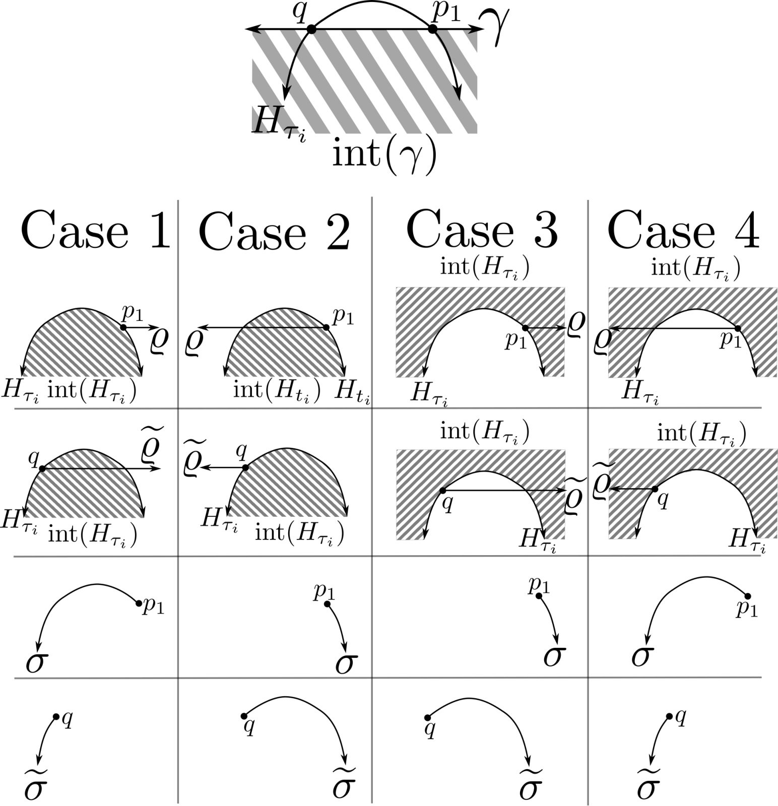
If is generated from , then we follow the above procedure, but in reverse. That is, if the Reidemeister move between and creates two intersection points of which one is an endpoint of , then we follow the above steps to produce a vertex . Note that for reasons analogous to those presented in the proof of Lemma 2.12, both endpoints of cannot be created by the Reidemeister move between and .
Before we complete the proof of Lemma 2.2, we prove some important properties of :
Lemma 2.13 (Properties of )
The graph has the following properties:
- 1.
For each set of edges , , and for each vertex generated from or , is the endpoint of exactly one edge in .
- 2.
All vertices generated from and all vertices generated from have degree 1; all other vertices have degree .
- 3.
There is exactly one vertex generated from , and one vertex generated from , and they correspond to the curves shown in Figure 21.
- 4.
If two vertices are joined by an edge, then there is a homotopy of closed curves between the curves corresponding to the vertices through closed curves of length at most . Furthermore, all of these curves contain .
Proof. The first statement is a result of the fact that the algorithm used to add edges takes any vertex generated from or from and produces a vertex , . Since we use this algorithm to add edges, there is an edge between and . Additionally, it is easy to check that this algorithm is symmetric in that the vertex will produce the vertex . Hence, each vertex is the endpoint of exactly one edge in .
The second statement results from the fact that, for each vertex that is generated from or from , is the endpoint of exactly one edge from or , respectively, and there is no other set which contains an edge that has as an endpoint. Thus, the degree is . For any vertex generated from with , is the endpoint of an edge from , and is also the endpoint of an edge from . Hence, it has degree .
The third statement follows from looking at the set of all valid subcurves at and . At each of these points, there are exactly two intersections between and , and so it is a simple exercise to look at each of the four subcurves and to show that the only ones that are valid are the ones depicted in Figure 21.
The last statement comes from examining how we add edges. In all of the cases, we are tracing two intersection points back or forth, and keeping track of one segment of that connects these points and one segment of that also connects these two points, which generates a continuous homotopy. Since both and are bounded in length by , taking a segment of one and joining it with a segment from the other has length at most
The fact that they all contain is a result of two observations. First, all subcurves at any respect , and so contain . Second, as a result of Lemma 2.8, no intersections between and lie in for any .

We can now prove Lemma 2.2.
Proof of Lemma 2.2. From Lemma 2.13, we have that there is only vertex generated from , and one vertex generated from . Additionally, they have degree , and all other vertices in have degree . As a result, we have that there is a path in from to . Let and be the subcurves that correspond to and , respectively. Due to the property of that edges represent homotopies over closed curves of length at most , there is thus a homotopy from to over such curves. Furthermore, every curve in this homotopy contains .
We now observe that is homotopic to over curves of length at most , and so we can homotope to over closed curves with the same length bound. All of these curves also contain .
The rest of the proof depends on whether contracts to a point inside or outside . If it contracts to a point outside , then we see that can be contracted to the point on through curves that contain . Since is contained in all curves in this homotopy up to , we conclude that is contained in every curve in this entire contraction.
If contracts to a point inside , then recalling that is the last point at which intersects , and is the point of tangential intersection at , we can homotope to through curves containing and which are bounded in length by . Since can also be homotoped to through such curves, this gives us a desirable homotopy from to . This completes the proof.
Finally, we illustrate this process using an explicit homotopy. This is shown in Figure 22.

2.2 Proof of Lemma 2.3
We now prove Lemma 2.3. Given a curve and a point , we want to show that we can contract through curves based at , and of length at most . The idea here is to employ a method similar to that used in this article to produce a contraction of the boundary of a Riemannian disc from a monotone contraction of that boundary. To do this, let be the point that contracts to. Join to via a minimal geodesic, and let be the last point of intersection between this geodesic and . This is depicted in Figure 23.

Our homotopy now works as follows. One should refer to Figure 24 for a visual reference. Let be the segment of the minimal geodesic that connects to entirely in the interior of . Let the length of be ; we of course have that , where is the diameter of the manifold. Let be a segment of that connects to which is of length at most . We now produce our contraction of in three parts. The first part is a homotopy from to the curve formed by traversing from to , following by traversing the entirety of from to , and then by traversing from back to . This homotopy consists of curves bounded in length by . Let us call this curve .

The second step is a homotopy from to the curve formed by traversing from to , then from to , then from back to , then from back to . Let us call this curve . This homotopy, , is defined on the interval , where (as above) is the length of . For each , let be the segment of from which has a length of . Since is monotone, there is exactly one curve corresponding to a curve in the homotopy which has the property that it goes through if , and that it goes through the endpoint of which is not if . Now, we define to be the curve formed by traversing , then , then , then , then . Since is monotone, this produces a continuous homotopy of piecewise smooth simple curves of length at most .
The third step is that we homotope to the point by contracting it in the obvious way; since it is a curve traversed forward from to to and then backward from to to , it is obvious how to do this without exceeding a length bound of .
By concatenating the above homotopies, we get a homotopy of closed curves with the desired properties, completing the proof.
Acknowledgements: This work was supported in part by an NSERC Discovery Grant (Rotman), by NSERC Postgraduate and Postdoctoral Scholarships (Chambers), and by an Ontario Graduate Scholarship (Chambers). This paper was partially written during the authors’ visit of the Max-Planck Institute for Mathematics in Bonn. The authors would like to thank the Max-Planck Institute for its kind hospitality.
This work is based on Chambers’ doctoral work. The authors would like to thank Arnaud de Mesmay, Erin W. Chambers, and Tim Ophelders for finding an error in an earlier version of this article.
References
- [BS] F. Balacheff, S. Sabourau, Diastolic and isoperimetric inequalities on surfaces, Ann. Sci. École Norm. Sup. 43 (2010), 579-605.
- [CL1] G. R. Chambers, Y. Liokumovich, Converting homotopies to isotopies and dividing homotopies in half in an effective way, Geom. Funct. Anal., vol. 24 (2014), 1080-1100.
- [CL2] G. R. Chambers, Y. Liokumovich, Existence of minimal hypersurfaces in complete manifolds of finite volume, preprint, arXiv:1609.04058.
- [C] C. B. Croke, Area and the length of the shortest closed geodesic, J. Diff. Geom. 27 (1988), 1-21.
- [FK] S. Frankel, M. Katz, The Morse landscape of a Riemannian disc, Ann. Inst. Fourier, Grenoble 43, 2 (1993), 503-507.
- [Gr] M. Gromov, Asymptotic invariants of infinite groups in Geometric Group Theory, v. 2, 1-295, London Math. Soc. Lecture notes Ser., vol. 182, Cambridge Univ. Press, Cambridge, 1993.
- [LNR] Y. Liokumovich, A. Nabutovsky, R. Rotman, Contracting the boundary of a Riemannian -disc, preprint, arXiv:1205.5474.
- [L1] Y. Liokumovich, Spheres of small diameter with long sweep-outs, Proc. Amer. Math. Soc. 141 (2013), 309-312.
- [L2] Y. Liokumovich, Surfaces of small diameter with large width, preprint, math arXiv:1307.2306, to appear in Journal of Topology and Analysis, 2013.
- [NR1] A. Nabutovsky, R. Rotman, Linear bounds for lengths of geodesic loops on Riemannian -spheres, J. Diff. Geom. 89 (2011), 217-232.
- [NR2] A. Nabutovsky, R. Rotman, Linear bounds for lengths of geodesic segments on Riemannian -spheres, J. Topol. Anal. 05, 409 (2013), 409-438.
- [NR3] A. Nabutovsky, R. Rotman, Length of geodesics and quantitative Morse theory on loop spaces, Geom. Funct. Anal., vol. 23 (2013), 367-414.
- [P] P. Papasoglu, Contracting thin disks, preprint, math arXiv:1309.2967.
| Gregory R. Chambers | Regina Rotman |
| Department of Mathematics | Department of Mathematics |
| University of Chicago | University of Toronto |
| Chicago, Illinois, 60637 | Toronto, Ontario M5S 2E4 |
| USA | Canada |
| e-mail: chambers@math.uchicago.edu | rina@math.utoronto.ca |