UAB-FT-744
Higgs Bosons in Extra Dimensions†
Mariano Quiros
Department of Physics, CERN Theory Division,
CH-1211, Geneva 23, Switzerland
and
Institució Catalana de Recerca i Estudis
Avançats (ICREA)
Institut de Física d’Altes Energies, Universitat Autònoma de Barcelona
08193 Bellaterra, Barcelona, Spain
Abstract
In this paper, motivated by the recent discovery of a Higgs-like boson at the LHC with a mass GeV, we review different models where the hierarchy problem is solved by means of a warped extra dimension. In the Randall-Sundrum model electroweak observables provide very strong bounds on the mass of KK modes which motivates extensions to overcome this problem. Two extensions are briefly discussed. One particular extension is based on the deformation of the metric such that it strongly departs from the AdS5 structure in the IR region while it goes asymptotically to AdS5 in the UV brane. This model has the IR brane close to a naked metric singularity (which is outside the physical interval) characteristic of soft-walls constructions. The proximity of the singularity provides a strong wave-function renormalization for the Higgs field which suppresses the and parameters. The second class of considered extensions are based on the introduction of an extra gauge group in the bulk such that the custodial symmetry is gauged and protects the parameter. By further enlarging the bulk gauge symmetry one can find models where the Higgs is identified with the fifth component of gauge fields and for which the Higgs potential, along with the Higgs mass, can be dynamically determined by the Coleman-Weinberg mechanism.
†Invited Review Paper submitted to Int. J. Mod. Phys. A special issue on ”Extra Dimensions versus Collider Physics”
1 Introduction
The discovery of the Higgs boson [the last missing ingredient of the Standard Model (SM)] at the LHC by the ATLAS [1] and CMS [2] collaborations, with a mass GeV, has now completed the Standard Model (SM) picture and made a big progress in clarifying the mechanism of electroweak symmetry breaking (EWSB). Although its nature, perturbative [as in the original Brout-Englert-Higgs (BEH) mechanism] versus non-perturbative [as in QCD], is not yet fully unveiled, everything seems to point towards a perturbative mechanism in the SM, although the accuracy of experimental data is not yet enough to rule out physics Beyond the Standard Model (BSM). Moreover from the theoretical point of view such electroweak vacuum would not be stable under quantum corrections (also known as hierarchy problem) which contribute to the Higgs mass with quadratically divergent radiative corrections, provided that we consider the SM as an effective theory. In particular the top quark contributes to the Higgs self-energy as
| (1.1) |
where is the SM cutoff. In the absence of any tuning this implies an upper bound on the cutoff scale as
| (1.2) |
and therefore beyond this cutoff there should exist new physics to stabilize it. Uncovering the nature of the electroweak symmetry breaking should amount to uncovering the kind of new physics (if any) which stabilizes the electroweak vacuum!
In fact there are two main avenues for solving the hierarchy problem depending on whether we consider the Higgs as an elementary scalar (perturbative EWSB) or a composite state (non-perturbative EWSB). The paradigm of perturbative EWSB which solves the hierarchy problem is supersymmetric theories, where there is an extra symmetry (supersymmetry) and extra matter (sfermions, gauginos and Higgsinos) with couplings dictated by supersymmetry such that there are extra contributions to the Higgs mass which cancel its quadratic sensitivity on the scale. For instance there is an extra scalar boson with the same quantum number of the top quark (the stop) whose contribution cancels that of the quark top in Eq. (1.1). This is not the solution we will cover in this review article.
The hierarchy problem is also solved provided that at some scale the Higgs dissolves, and the theory of its constituents is at work. This case is similar to QCD where the pions dissolve into quarks and gluons beyond . In fact the compositeness scale acts as a cutoff of quadratic divergences. The typical example of compositeness is Technicolor. Modern theories of compositeness involve an extra dimension through the Anti-de-Sitter/Conformal-Field-Theory (AdS/CFT) correspondence [3]. This provides an extra motivation to study models in a warped extra dimension, the paradigm being the original five-dimensional (5D) Randall-Sundrum (RS) setup [4] which, in particular, we will review in this article whose contents are as follows.
In section 2 we will consider some general features of the 5D Standard Model propagating in the bulk of an extra dimension with an arbitrary warp factor. In section 3 we will provide general expressions for the oblique electroweak observables , , and for a general warp factor and a general bulk Higgs profile. For completeness we will also provide general expressions for the observables , which appear when we use different localization of bulk fermions in order to solve the flavour problem. This mechanism would also generate flavor-changing neutral currents (FCNC) and CP violating effective operators. However, as the issue of fermion flavor will not be covered in this review, we will concentrate in the following sections on constraints from universal corrections. In section 4 we will consider the case of AdS5, the original RS proposal. We will deduce the constrains on the Higgs profile in order to solve the hierarchy problem and the constraints imposed on the mass of the first KK excitation of gauge bosons from electroweak precision tests (EWPT). In particular we will find that, depending on the Higgs localization, EWPT impose lower bounds TeV, which are outside the LHC reach and would recreate a little hierarchy problem. This problem has motivated extensions of the RS model in order to overcome those bounds. Two possibilities have been reviewed here. The first possibility, considered in section 5, consists in introducing a dilatonic scalar such that the warping of the fifth dimension is strongly modified near the IR brane while it behaves as AdS5 near the UV region. In fact we are using soft-wall metrics such that the naked singularity is regularized by the IR brane. The closer the IR brane to the naked singularity the stronger the effect. The hierarchy problem imposes constrains on the Higgs profile which are stronger than those in the RS case. It turns out that there is a strong renormalization wave equation for the Higgs field such that there is an extra suppression on electroweak observables. This renormalization effect effectively depends on the departure of the IR metric from AdS5. Electroweak constraints then provide mild bounds as TeV depending on the values of the parameters defining the metric. The second way out to the problem of strong electroweak constraints on the pure RS model has been reviewed in section 6. It consists in adding a gauge symmetry in the bulk which contains the custodial symmetry group and thus guarantees that the SM tree-level condition is respected, thanks to the cancellations induced by the extra states required to accommodate matter in multiplets, while there is a tree-level contribution to the parameter. In this case the one-loop contribution to the parameter coming from the top quark and its partners should be considered. Finally EWPT impose the condition TeV. Moreover we also review the case where one embeds the custodial group into a larger group such that the Higgs degrees of freedom can be identified with the fifth components of the 5D gauge fields along the broken generators: these models are dubbed Gauge-Higgs Unification models. In Gauge Higgs Unification the Higgs potential and the Higgs mass can be obtained dynamically by the Coleman-Weinberg mechanism. Different models then essentially differ by the bulk group containing and by the subgroup surviving at the IR brane and they are thus dubbed with different names, e.g. minimal composite Higgs model for . Finally section 7 contains our conclusions which essentially will depend on future experimental results on the LHC13-14 running where Higgs data on production strengths will be delivered with more accuracy. In particular they should clarify whether there are any departures with respect to the Standard Model predictions in the different channels.
2 Standard Model in Warped Extra Dimensions
We will now consider the Standard Model propagating in a 5D space with an arbitrary metric such that in proper coordinates the line interval is: where . This anstaz is the most general one consistent with Minkowski space-time in 4D. We define the 5D gauge bosons as , where and , and the SM Higgs as
| (2.1) |
where the matrix contains the three 5D SM fields . The Higgs background as well as the metric are for the moment arbitrary functions and they will be specified later on. We will consider the 5D action for the gauge fields and the Higgs field as:
| (2.2) | |||||
where is the 5D potential, () the 4D brane potentials, the induced metric at the brane located at , and we will choose conventionally . The bulk and brane potentials will depend in general, not only on the Higgs but also on possible stabilizing (dilatonic) fields in the theory. From here on we will assume that is quadratic in . Electroweak symmetry breaking will be triggered on the IR brane. We thus choose the brane potentials as
| (2.3) |
The effect of the warp factor can be encoded in the parameter defined as
| (2.4) |
and in order to solve the hierarchy problem has to be chosen such that for a Planckian value of , is at the TeV scale: i.e. .
One can then construct the 4D effective theory out of (2.2) by making the KK-mode expansion where . The functions satisfy the equations of motion (EOM) they are normalized as , and satisfy the Neumann boundary conditions (BC) We have defined the 5D -dependent gauge boson masses as where , and , , are the 5D and couplings respectively. Only the lightest mass eigenvalue will be significantly affected by the breaking so we simplify our notation by defining for the zero modes and for the higher modes (). An approximated expression is given by [5, 6, 7, 8]
| (2.5) |
The background is determined from the bulk EOM and BC
| (2.6) |
while for the Higgs fluctuations, the bulk EOM and BC are
| (2.7) |
With our choice (2.3) of boundary potential the UV boundary conditions for the background and fluctuations are the same, and for a quadratic bulk Higgs potential the Higgs wave function for () is thus proportional to . For small Higgs mass this will still be a good approximation to the exact wave function. This means that the 5D VEV will be carried almost entirely by the zero mode.
We can then write an effective theory by the decomposition and calculate the effective Lagrangian for the mode . In fact the SM Lagrangian is where the SM parameters and are related to 5D quantities by [6]
| (2.8) |
and
| (2.9) |
The usual SM expressions for the Higgs VEV and Higgs mass follow straightforwardly. The quantity is an additional wave function renormalization depending on both the gravitational and Higgs backgrounds. As we will see in the next section (see also Refs. [5] and [6]), a sizable suppresses the () parameter by two (one) powers of , which leads to a corresponding reduction in the value of from EWPT. Moreover we see here that the parameter , or equivalently the Higgs mass, is further reduced with respect to by a factor which in turn reduces the required amount of fine-tuning in the factor .
3 Electroweak precision observables
There are three experimental input parameters, usually referred to as , and parameters [9], which appear in theories where fermions couple in a universal way: they are called oblique parameters. In models with a gap between the electroweak and new physics scales the parameter is expected to be small since it corresponds to a dimension eight operator. On the other hand, there are other dimension six operators unrelated to electroweak breaking which in some models can have sizable coefficients. It has thus been suggested to instead consider the set , , and as a more adequate basis for models of new physics [10]. They are defined as
| (3.1) |
where is the electromagnetic gauge coupling defined at the -pole mass.
In theories with a Higgs mode of mass one can relate , , and to the coefficients of the dimension six operators
| (3.2) |
in the effective low energy Lagrangian respectively. These coefficients can be obtained in the effective theory by integrating out the KK-modes from where one can write the general expression [6]
| (3.3) |
where the function , determined by the localization properties of fermion with a 5D Dirac mass equal to , is given by
| (3.4) |
and we are assuming for the moment universal localization of all fermions. Similarly the localization properties of the Higgs field are determined by the function given by
| (3.5) |
In the case of UV-localized fermions we can see that . This is the usually considered case as first and second generation fermions, which are the relevant ones for most of the precision observables, are light and then for them. In the case of flat fermions, i.e. we have that so that but still is non-vanishing and it has to be taken into account for phenomenological purposes. Finally for the case of IR localized fermions () is localized towards the IR brane. As also the Higgs is localized towards the IR brane in order to solve the hierarchy problem (as we will see later on) it turns out that also is localized towards the IR brane and thus the difference , along with the parameter, tends to be small, but still the contribution from the other parameters , and can give very strong phenomenological constraints.
If fermion localization is not universal, i.e. if the constants are not equal for all fermions, as it is usually the case when one wants to provide a theory of fermion flavor from fermion localization, then non-oblique corrections are also generated. In particular the most important of those non-oblique operators give corrections to the coupling. The calculation was done in Ref. [11] with the result
| (3.6) |
where and and the integrals and are
| (3.7) |
As the bounds from the coupling depend, to a large extent, on the different localization of bulk quarks in order to reproduce the texture of quark masses and mixing angles, a topic which will not be covered by this article, we will concentrate on the case of oblique corrections and we will assume that approximately first and second generation quarks are localized towards the UV brane, in which case in Eq. (3.1). We can then readily compute the electroweak observables as
where
| (3.9) |
The dimensionless integrals are expected to be of the same order. In particular one expects . We see that is enhanced by a volume factor and thus it is expected to be the leading observable, while carries no power of the volume and it is thus the next to leading one. On the other hand the and parameters are suppressed with one (two) additional volume factor(s) as compared to ().
4 AdS5
The paradigm of warped space was first introduced by Randall and Sundrum [4] and it consists in a 5D AdS space, i.e. with a metric given by , with two branes localized at (the UV brane) and at (the IR brane). In this case the wave function of KK gauge bosons is obtained analytically (neglecting the small correction from EWSB) as
| (4.1) |
where and are Bessel functions and the constant and the mass eigenvalues come from imposing the UV and IR boundary conditions. is the AdS curvature and it is warped down to the TeV scale by while the mass of the first KK mode is related to by the relation: with .
4.1 The hierarchy problem
The original solution to the hierarchy problem comes for a Higgs field fully localized in the IR brane [4]. In this case we can write the Higgs action as
| (4.2) |
where is the induced metric at the IR brane. After making the rescaling the action can be written as
| (4.3) |
from where it can be seen that a Planckian value of is brought to the electroweak value as . In fact this result is completely general: any mass parameter in the IR brane get rescaled in the same way as . This is the original warped solution to the hierarchy problem.
Of course having a Higgs localized on the IR brane is not the only solution to the hierarchy problem as we will see next. In fact, for a quadratic bulk Higgs potential as , to determine whether the hierarchy problem is successfully solved by a profile of the form with small let us write the solution of our Higgs profile subject to a generic electroweak symmetry preserving UV-boundary condition (2.6) as
| (4.4) |
For no fine-tuning is necessary in order to keep only the first term, since near the IR brane (where EWSB occurs) the second term is always irrelevant. On the contrary, for , the second term would be dominating and one needs to fine-tune in order to maintain the solution . This fact has a simple holographic interpretation: since the hierarchy problem is solved by the Higgs compositeness for , but not for (see Ref. [12] for a more detailed discussion). One can now quantify using 5D techniques the required amount of fine-tuning for by imposing and assuming that the second component in (4.4) is similar to the first component at the IR brane, we can easily quantify the amount of required fine-tuning as
| (4.5) |
In fact Eq. (4.5) yields, for , the same amount of fine-tuning which is required in the Standard Model, while it decreases linearly in the exponent along the interval .
In this theory the function in Eq. (2.8) is given by and the value of the Higgs mass from (2.8) is given by
| (4.6) |
Then the required amount of fine-tuning for obtaining a light Higgs boson can be quantified by imposing as
| (4.7) |
This would correspond to a 1% fine-tuning for TeV. However, as we will see in the next section, electroweak observables put very strong lower bounds on the value of , which translate into a more severe tuning for a Higgs with a mass GeV as experimentally observed at the LHC. For instance for TeV the required tuning is : this is the typical tuning in the RS model and it would create a little hierarchy problem associated with the KK masses.
4.2 Electroweak constraints
For the AdS5 metric it is very simple to compute analytically the , , and parameters from Eq. (3.3). In fact they are given by [5]
| (4.8) |
from where we can see that, as foreseen for general metrics, the parameter is enhanced by the compactification volume and it is thus the most constraining one out of the oblique parameters. On the other hand does not depend on the volume and it is the next to leading parameter, while and are suppressed by the compactification volume and they are thus usually negligible in phenomenological applications. In the following we will just consider the leading and parameters.

Comparison of oblique parameters with experimental data provide in general lower bounds on the KK masses . In Fig. 1 we show the 95% CL (68% CL) allowed region, for a Higgs mass GeV, which corresponds to the region inside the outer (inner) ellipse [13]. The dots and interpolating lines correspond to the predictions of the RS model for [right (red dots) dashed line] and for the limit [left (blue dots) dashed line]. The values for the (red) dots correspond to TeV where the dots are spaced by TeV, and TeV corresponds to the dot touching the 95% CL ellipse while TeV corresponds to the most outer dot. Similarly the line corresponding to an IR localized Higgs corresponds to TeV where the dots are spaced by TeV and TeV is the dot touching the 95% CL ellipse while TeV is the furthest dot on the blue line.
Therefore from the results of Fig. 1 we conclude that, for an IR localized Higgs, compatibility with EWPT provides the lower bound TeV at the 95% CL, while the bound improves when we delocalize the Higgs from the IR brane as much as possible. The solution of the hierarchy problem then implies that and we get the global bound TeV at the 95% CL.
The model described in this section has of course the capability of providing a theory of quark and lepton flavor by adjusting the constants to fit all fermion masses and mixing angles contained in the CKM [11] and the PMNS [14] matrices. This process is not for free because it originates extra FCNC and CP violating operators which further constrain the model parameters. These developments are outside the scope of this review article and will be covered in Ref. [15].
However it goes without saying that the RS model we have just presented is not phenomenologically appealing as:
- •
KK modes are not accessible to LHC.
- •
It recreates a little hierarchy problem.
The ways of relaxing the strong constraints from the electroweak observables consist obviously in modifying the model as will be explained in the next sections. We will see that there are mainly two options to overcome this problem:
- •
Either one can deform the metric in the IR region in such a way that it is still AdS5 asymptotically near the UV brane (AAdS5). As we will see the deformation can create a naked singularity of the metric. By localizing the IR brane close enough to the singularity its effect will damp the impact of the -observable on the lower KK mass bounds. In this kind of background we do not need to add extra matter and/or gauge bosons and we can just propagate the Standard Model content in the bulk.
- •
Or another option is to keep the AdS5 geometry everywhere but to extend the gauge group and matter content in the bulk. In particular we will see that introducing a local group in the bulk (which holographically corresponds to a global custodial symmetry group in 4D) the -observable can be protected from radiative corrections and again the bounds on KK mass observables are mitigated. We will call these Custodial Models.
Let us finally mention another way of relaxing constraints from electroweak observables (although it will not be covered in this review). It consists [16, 17] in introducing brane-localized kinetic terms for gauge bosons and/or fermions. These terms will be generated anyway from radiative corrections at the orbifold fixed points (where branes are localized). The shortcoming of this approach is that the required strengths for overcoming the constraints from electroweak observables are much larger that the natural values generated by radiative corrections.
5 Standard Model in singular backgrounds
Let us assume the 5D background metric is such that there is a naked singularity at the point and that we locate the IR brane at , a short distance away from the singularity, i.e. with . In principle this can be done by introducing a stabilizing diatonic field with potentials at the UV and IR branes fixing appropriates values and . In this case as the metric has a singularity at the integral defining the Higgs wave function renormalization in Eq. (2.8) is dominated by the region near and it is thus enhanced with respect to the RS value. Constructions based on singular backgrounds are usually dubbed soft-walls [18, 19, 20, 21, 22].
One particularly simple construction was proposed in Ref. [23] (see also Ref. [24]) where the metric and dilaton profiles were given by
| (5.1) | |||||
| (5.2) |
where is a real parameter and we are using the normalization . As we can see from (5.2) near the UV brane () the metric coincides with that of AdS5 while when there is a large departure from the AdS5 metric: this is the typical behaviour of AAdS5.
As we said we are assuming that the brane dynamics fixes the values of the field on the UV and IR branes respectively. The interbrane distance, , as well as the location of the singularity, , are related to the values of the field at the branes by the following simple expressions:
| (5.3) |
which shows that the required large hierarchy can naturally be fixed with values of the fields and , . Note that due to its exponential dependence on , can be small or, in other words, the IR brane can naturally be located very close to the singularity. One interesting feature of this model is that the value of the volume required to solve the hierarchy problem is smaller than in the model with AdS5 as it is shown in Fig. 2 where we plot as a function of for (which we will be using in the rest of this paper) and .
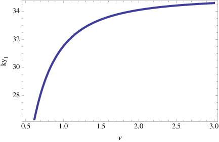
We see that for values of there can be a considerable reduction on the volume . On the contrary for large values of the RS-limit is recovered and consequently the volume .
The EOM, e.g. for the gauge boson KK modes, cannot be solved analytically in such a complicated background so that all the calculations have to be performed numerically. A useful fit relating the parameter with the mass of the first KK excitation is given by Ref. [5]
| (5.4) |
5.1 The hierarchy problem
The bulk Higgs potential is written as
| (5.5) |
and the coefficients of the two operators and can be considered as independent parameters. However since the parameter can be traded by a global shift in the value of the field, or in particular by a shift in its value at the UV brane , for simplicity we will fix its value to hereafter. We can now write the general solution to Eq. (2.6) as
| (5.6) |
The two integration constants are fixed from the boundary conditions in (2.6) derived from the boundary potentials given in Eq. (2.3).
In order to determine whether the hierarchy problem is successfully solved by a profile of the form with small let us write the solution of our Higgs profile subject to a generic electroweak symmetry preserving UV-boundary condition as
| (5.7) |
As in the AdS5 case, for 11 1 Note that while for RS, for the singular metric (5.2) as we will see next. the solution will be fine-tuned due to the exponential enhancement in the integrand. We can rewrite the solution as
| (5.8) |
where the function is given by
| (5.9) |
Note that is defined as a complex function but its imaginary parts cancels in (5.8) leading to a real function. One should view as the generalization of in the RS case. In order to keep the exponential solution without the need of any fine-tuning we must require the function to be small in absolute value. Since is a monotonically increasing function of it will be enough to inspect which will be a measure of the fine-tuning required in in order to keep the exponential solution. In particular the absence of fine-tuning requires roughly . The contour plot for in the plane () with is plotted in the solid (red) line of Fig. 3 22 2 In the considered region of the parameter space we can see that the value satisfies the fine-tuning condition for all values of so that fixing is just a conservative assumption..

In fact the allowed (fine-tuned) region which corresponds to () is above (below) the solid line. We see that in the limit (where the RS metric is reached) the bound on corresponds to as in the case of AdS5 metric.
The Higgs mass is given by Eq. (2.8) as
| (5.10) |
so that the required fine-tuning to reproduce the experimental value GeV depends on the values of and . If we quantify the fine-tuning by imposing that then
| (5.11) |
so that the larger (the smaller) () the less fine-tuned is the theory. In particular the factor was one of the elements which increased the fine-tuning in the Higgs mass determination in the case of AdS5 as for . In the deformed metric of this section we can achieve values of which then lower the amount of fine-tuning. In particular in Fig. 3 we plot dashed contour lines of constant (on the right side), 1 (next curve, 2 (next curve) and 5 (on the left side). In the region allowed by the solution to the hierarchy problem (above the solid line) we see that, depending on the values of and , we can have values of as large as . The second factor which determines the degree of fine-tuning in fixing a light Higgs is the value of which is constrained by EWPT as we will see in the next section. In fact in the region where if TeV, as we will see next, then and there is no fine-tuning at all.
To analyze perturbative unitarization of the theory one can compute the coupling of the Higgs to gauge bosons and in particular one can prove that [6]
| (5.12) |
so a light Higgs unitarizes the theory in a similar way as the SM Higgs.
5.2 Electroweak constraints
For the singular metric of Eq. (5.2) the electroweak observables of Eq. () do not have an analytical expression. They have to be computed numerically. However in the region where is large enough we can approximate and by


| (5.13) |
We will check the accuracy of the approximation by defining the corresponding relative errors as
| (5.14) |
which we plot in Fig. 4 as a function of for and . We can see from the left panel of Fig. 4 that is a good approximation, within an error %, while from the right panel we see that approximates the exact value of only with errors %. The reason for the different accuracy of both observables is that the goodness of the approximation is governed by the size of , and is suppressed by two powers of while is suppressed only by one power of . The plots in Fig. 4 are valid for any value of .

In Fig. 5 we plot the values of the and parameters (using the exact numerical expressions) for , 33 3 For which there is no hierarchy problem in the considered region of the parameter space, see Fig. 2. and various values of , and we compare them with the region allowed by experimental data. Using the results from the plots in Fig. 5 we can see that the 95% CL bounds on considerably decrease with respect to their values in the RS model. In particular we can read from Fig. 5 the following bounds: 0.8 TeV (for ), 1.2 TeV (for ), 1.8 TeV (for ) and 10 TeV (for ). In fact for the value we essentially recover the results from the RS model as we can see in the solid lines of Fig. 5 which correspond to the RS model for the cases of and a fully IR localized Higgs .
We can understand the improvement from electroweak constraints in the soft-wall model by the different behaviour of the Higgs profile at the IR brane location (see e.g. Ref. [25]). In fact the normalized physical Higgs wave function is defined as
| (5.15) |
where is a normalization factor such that
| (5.16) |
As KK-modes are localized towards the IR brane it turns out that their overlapping with the Higgs excitations (and therefore their contribution to the electroweak observables and ) depends to a large extent on the values of the physical Higgs wave functions at the IR brane. In fact the values of the physical Higgs wave functions for the AdS5 and singular background (SW) satisfy the inequality (for a fixed ) if the singular background metric departs sufficiently from AdS5 at the IR brane. This property is exhibited in the left panel of Fig. 6 [the shadowed (yellow) region] where we plot as a function of for the fixed value . We have used for the RS case while we are using for the SW case consistently with the previous comments about the solution of the hierarchy problem. In this way our result is a conservative one, as from Fig. 3 we can see that values would be consistent with the solution to the hierarchy problem for values . Notice that the condition (shadowed region) is satisfied for where we expect deep deviations from AdS5 near the IR brane. Notice also that in both cases we have fixed the condition to solve the hierarchy problem so that for the SW case as we saw in Fig. 3. The profiles of the physical Higgs wave functions (for , , and ) and (with ) are plotted as functions of in the right panel of Fig. 6 where we can see that has a maximum at a value .


Implications at the LHC for this class of warped extra-dimensional models have been studied in Refs. [25, 26, 27]. These papers discuss both the production of electroweak and strong Kaluza-Klein gauge bosons. Only signals involving the third generation of quarks seem to be feasible in order to probe this scenario.
As we had tree-level contributions to the oblique parameters we did not pay too much attention for the moment to radiative corrections as they are expected to be subdominant, provided they are calculable. This issue has been discussed in several papers [28, 25] and here we just review the main argument, which is purely based on dimensional analysis. We will exemplify this analysis with the and parameters. As there is no custodial symmetry protecting the parameter we can write the bulk effective Lagrangian terms as
| (5.17) |
where is the 5D cutoff scale and we assume canonical dimensions for the gauge fields, which can be done by defining the kinetic terms as and . The prefactors come just from the dimension of the Higgs propagating in the bulk and the dimensionless coefficients and are related to the and parameters.
The leading one-loop diagram contributing to the parameter is that given in Fig. 7 where the top quark is exchanged in the loop
with a 5D coupling with dimension 44 4 This comes from the bulk interaction term with .. The contribution from the diagram in Fig. 7 is then proportional to times the 5D integral over momenta. As it follows that the term in the momentum integral proportional to has dimension -1 and it is thus finite. If we subtract the top-quark zero mode the result should be controlled by the scale [25]. This result only holds at one loop. In fact if we consider the two-loop diagram of Fig. 8
we get its contribution to be proportional to and thus as the momentum integral has dimension 0, and so it is logarithmically divergent (still calculable). Only the three loop diagram, proportional to , will be linearly sensitive to the cutoff and thus non calculable but tiny.
A similar analysis can be done for the parameter. At one-loop it is generated by the diagram in Fig. 8
which is proportional to . As it means that the momentum integral has dimension -1 and it is thus finite. At two-loop we consider the diagram of Fig. 10
which is proportional to and from we see that the corresponding loop integral is logarithmically divergent and thus calculable. Again only the three loop diagrams, proportional to , will be linearly sensitive to the cutoff but with a huge loop suppression.
Let us finally notice that these results are valid only for a bulk propagating Higgs. If the Higgs is localized on the IR brane, and so it has mass dimension , then we can write the tree-level effective Lagrangian as
| (5.18) |
and the localized top Yukawa coupling 55 5 From the brane localized Yukawa interaction with . has dimension . In this case the diagram of Fig. 7 contributing to the parameter is proportional to with dimension such that the term proportional to in the calculation of the diagram has dimension +2, which means a quadratic sensitivity to the cutoff and the corresponding contribution not being computable. Likewise the diagram of Fig. 9 contributing to the parameter is proportional to with dimension , which means a logarithmic sensitivity to the scale of the parameter, while the two loop diagram of Fig. 10 proportional to , with dimension , yields a quadratic sensitivity.
In this section we have seen how in models with the Standard Model propagating in the bulk of the extra dimension we can cope with the experimental values of the electroweak observables by departing from the AdS5 geometry near the IR brane. Of course in these models we can also fix the quark and lepton structure of masses and mixing angles by the different localization of fermions in the bulk by means of different 5D Dirac masses. As in the RS model this process creates FCNC and CP violating operators which should be made consistent with their experimental bounds [11, 25, 14]. This issue will not be considered here, as it will be reviewed elsewhere [15].
6 Custodial Models
Another way of enforcing the strong constraints imposed by the parameter is to promote the custodial symmetry to a gauge symmetry in the bulk. This idea was put forward in Ref. [29]. In particular the construction proposed there consisted in enlarging the electroweak gauge group in the bulk to (where ). The gauge group is then broken by boundary conditions in the UV brane to the Standard Model gauge group (where ) while it remains unbroken in the IR brane. We can thus impose Neumann () boundary conditions on the brane [] to keep the corresponding gauge boson massless and Dirichlet () boundary conditions [] to give it an (infinite) mass. Thus the required boundary conditions on the (UV, IR) branes at are 66 6 All gauge couplings here are 5D. Their 4D counterparts are defined according to the usual formula: .
| (6.1) |
and the 5D covariant derivative becomes in terms of the new gauge fields
| (6.2) |
where and are the couplings, is the coupling, the coupling and is the charge with the mixing angle given by
| (6.3) |
Since we have enlarged the bulk gauge symmetry the right-handed fermions should be promoted to doublets under . However since we are breaking this symmetry through the UV boundary conditions only one of the components of the doublet should have a zero mode while the other should not have any. This means that to have two zero modes we need to double the number of doublets with different boundary conditions. For instance for the right-handed up quarks we will need to doublets
| (6.4) |
where only the untilded fields possess a zero mode. In fact since we are breaking through the orbifold boundary conditions, one component of must be even (with a zero mode) and the other odd (no zero mode). This doubling on the number of fields is only required in the quark sector as in the lepton sector for the doublet
| (6.5) |
only the field needs to possess a zero mode.
Finally the Higgs is considered as a bidoublet under , with a potential localized at the IR brane such that it provides a minimum at GeV and with a small ratio to the warped down curvature scale . The Yukawa couplings to fermions are written by the IR localized terms .
As the KK-modes are localized towards the IR boundary and both the bulk and the IR boundary respect exactly the custodial symmetry (even for ) the vanishing of the parameter is enforced by the custodial symmetry. In fact the detailed calculation [29] shows that there is a tree-level cancellation between the contribution from and and the terms enhanced by vanish. This yields at the tree level, and assuming that light fermions are localized at the UV brane, the following expressions for and
| (6.6) |
where .
At the one-loop level, on top of the usual Standard Model leading contribution from the top quark zero mode, the dominant contribution comes from a loop where the KK-modes and are exchanged, as in the diagrams of Figs. 7 and 11 where big dots correspond to Higgs insertions .
In fact after summation over all KK-modes in the loop, and considering , Ref. [29] gets the numerical result
| (6.7) |
where is the mass of the first KK-mode for gauge bosons. In Fig. 12 we plot the values of the and parameters

from Eqs. (6.6) and (6.7) and we compare them with the experimental data on electroweak observables. The dots correspond to values of TeV with an interval between points of TeV. From there one can infer the lower bound of TeV at the 95% CL.
Up to this point we considered the Higgs as a fundamental field but there are theories where the Higgs is not introduced as an extra matter because:
- •
- •
Or the Higgs is the fifth component of the gauge bosons of an enlarged bulk gauge symmetry.
In these cases EWSB is generated dynamically. In particular the latter possibility is being explored in depth at present and it is dubbed Gauge-Higgs Unification (GHU) [33, 34, 35, 36, 37].
GHU is actually an alternative to supersymmetry [38], where the (5D) gauge symmetry in the bulk protects the mass of extra-dimensional components of gauge bosons [39, 40, 41]. This solution to the hierarchy problem requires an extended gauge group with respect to the SM gauge group. It can be constructed in flat or warped space, although in warped space the GIM-RS mechanism protects the theory with differently localized fermion fields from huge flavor violation, which otherwise would require severe constraints on the mass of KK modes [42]. The four-dimensional components of 5D gauge bosons of with boundary conditions span the four-dimensional gauge group while the fifth components , with boundary conditions 77 7 Correspondingly and have boundary conditions., contain the four-dimensional Higgs (and Goldstone boson) fields in a number equal to the number of Pseudo Goldstone Bosons (PGB) which are left out in the four dimensional theory.
In general will be broken by boundary conditions to () on the UV (IR) brane. For the number of PGB is so different models differ by different choices for and . Some models [43, 44, 45] are defined in the table below.
| Model | # PGB () |
|---|---|
| SO(4)/SO(3) | 6-3=3 (Higgsless SM) |
| SU(3)/SU(2)U(1) | 8-4=4 |
| SO(5)/SO(4) | 10-6=4 |
| SO(6)/SO(5) | 15-10=5 ( + singlet) |
| SO(6)/SO(4)SO(2) | 15-6-1=8 |
The first model in the table, , contains the SM Goldstone bosons and thus it is a Higgless model. This kind of models have been excluded by the discovery at the CERN LHC of the Higgs-like boson with mass GeV. The second model presented in the table, , is sometimes studied as a toy model as it contains the SM Higgs on top of the SM Goldstone Bosons. In order to accommodate quark hypercharge it has to be accompanied by factor(s). It does not contain the custodial symmetry on the IR brane and thus the parameter is not protected for it. The rest of the models in the table contain the custodial subgroup on the IR brane and so their contribution to the parameter is protected. In particular the third model on the table, , [usually accompanied by a common factor ] is the minimal model which contains the custodial subgroup and thus it is commonly dubbed as Minimal Composite Higgs Model (MCHM) [44].
In the dual theory is characterized by the spontaneous breaking scale such that the expansion parameter in the theory is
| (6.8) |
The parameter controls perturbative unitarity through a relation similar to Eq. (5.12). However unlike in the models presented in previous sections with a fundamental scalar Higgs, where the parameter , in the models presented in this section depends on and can thus be considered as a free parameter. For instance in the limit the SM result is obtained and the Higgs unitarizes the theory without the need of any extra particle. On the other extreme in the Technicolor limit all unitarity must be provided by new TeV resonances at scales close to the electroweak scale. For intermediate values of unitarity must be partially restored by resonances at scales which depend on the value of .
As we are identifying the Higgs field with the fifth component of a gauge field, 5D gauge invariance prevents any bulk potential term at the tree level. However a Coleman-Weinberg potential is generated at one-loop level which can be responsible for EWSB. This potential can be written on general grounds in the usual way
| (6.9) |
where are the mass eigenvalues of KK modes of the different bulk fields in the presence of the Higgs background . The potential (6.9) was computed and given an analytic approximation in Ref. [46] using holographic methods in arbitrary gravitational backgrounds. In particular, in the AdS5 background it can be written as
| (6.10) |
where are the degrees of freedom for the different fields ( for gauge bosons, =-4 for fermions) and the corresponding couplings ( for gauge bosons, for the top quark). As for they are representation dependent order one constants: are eigenvalues of the symmetric mass matrix and the Higgs decay constant is given by
| (6.11) |
We can see that the potential (6.10) is periodic. The gauge components have a minimum at while the fermionic components have a maximum at and thus trigger EWSB and a minimum at , i.e. . Depending on the number of bosonic and fermionic degrees of freedom one can generate a non-trivial minimum in between. This situation has been exemplified in the plot of Fig. 13 where we have considered a case with () and the number of bosonic and fermionic degrees of freedom as required to generate such an intermediate minimum.

Moreover one can consider in general an effective theory [47] parametrized by , which measures the degree of compositeness of the Higgs. In this theory all Higgs couplings (cubic, quartic, , …) depart from the SM values by quantities which are proportional to . These models have been confronted to EWPT and direct searches [48]. The former ones provide the strongest constraints which yield typical bounds at 99% CL in the absence of additional contributions to the and parameters.
7 Conclusions
It is clear at this moment that the next step in Higgs physics belongs to the LHC, in particular to the ATLAS and CMS collaborations, so that confronting in great accuracy different theories on electroweak symmetry breaking with experimental data should wait till LHC13-14, when more statistics will be accumulated and Higgs production rates will be given more accurately. In particular if theories with extra dimensions are the solution to the hierarchy problem the Higgs is expected to be composite to some extent, which should leave imprints in experimental data and in particular on Higgs production strengths. In any case if a warped space is a solution of the hierarchy problem it requires a UV completion as the theory becomes strongly coupled at some multi-TeV scale. But even if it turns out that the detection of the degree of Higgs compositeness be outside the LHC accuracy it is clear that a confirmation of the extra dimensional nature of the space should be made by direct detection of the extra states that all these theories predict: KK excitations, extra 4D matter (as the extra states required by the custodial models), …. So the main (obvious) conclusion is that from 2015 on, when LHC13-14 will restart operations, we should stay tuned.
Acknowledgments
Work partly supported by the Spanish Consolider-Ingenio 2010 Programme CPAN (CSD2007-00042) and by CICYT-FEDER-FPA2011-25948.
References
- [1] G. Aad et al. [ATLAS Collaboration], “Observation of a new particle in the search for the Standard Model Higgs boson with the ATLAS detector at the LHC,” Phys. Lett. B 710, 49 (2012) [arXiv:1207.7214 [hep-ex]].
- [2] S. Chatrchyan et al. [CMS Collaboration], “Observation of a new boson at a mass of 125 GeV with the CMS experiment at the LHC,” Phys. Lett. B 710, 26 (2012) [arXiv:1207.7235 [hep-ex]].
- [3] J. M. Maldacena, “The Large N limit of superconformal field theories and supergravity,” Adv. Theor. Math. Phys. 2, 231 (1998) [hep-th/9711200].
- [4] L. Randall and R. Sundrum, “A Large mass hierarchy from a small extra dimension,” Phys. Rev. Lett. 83, 3370 (1999) [hep-ph/9905221].
- [5] J. A. Cabrer, G. von Gersdorff and M. Quiros, “Warped Electroweak Breaking Without Custodial Symmetry,” Phys. Lett. B 697, 208 (2011) [arXiv:1011.2205 [hep-ph]].
- [6] J. A. Cabrer, G. von Gersdorff and M. Quiros, “Suppressing Electroweak Precision Observables in 5D Warped Models,” JHEP 1105, 083 (2011) [arXiv:1103.1388 [hep-ph]].
- [7] J. A. Cabrer, G. von Gersdorff and M. Quiros, “Improving Naturalness in Warped Models with a Heavy Bulk Higgs Boson,” Phys. Rev. D 84, 035024 (2011) [arXiv:1104.3149 [hep-ph]].
- [8] J. A. Cabrer, G. von Gersdorff and M. Quiros, “Warped 5D Standard Model Consistent with EWPT,” arXiv:1104.5253 [hep-ph].
- [9] M. E. Peskin and T. Takeuchi, “Estimation of oblique electroweak corrections,” Phys. Rev. D 46, 381 (1992).
- [10] R. Barbieri, A. Pomarol, R. Rattazzi and A. Strumia, “Electroweak symmetry breaking after LEP-1 and LEP-2,” Nucl. Phys. B 703, 127 (2004) [hep-ph/0405040].
- [11] J. A. Cabrer, G. von Gersdorff and M. Quiros, “Flavor Phenomenology in General 5D Warped Spaces,” JHEP 1201, 033 (2012) [arXiv:1110.3324 [hep-ph]].
- [12] M. A. Luty and T. Okui, “Conformal technicolor,” JHEP 0609, 070 (2006) [hep-ph/0409274].
- [13] J. Beringer et al. (Particle Data Group), Phys. Rev. D86, 010001 (2012) and 2013 partial update for the 2014 edition.
- [14] G. von Gersdorff, M. Quiros and M. Wiechers, “Neutrino Mixing from Wilson Lines in Warped Space,” JHEP 1302, 079 (2013) [arXiv:1208.4300 [hep-ph]].
- [15] G. von Gersdorff, ”Flavor Physics in Warped Geometries,”, to appear in this Special Issue.
- [16] H. Davoudiasl, J. L. Hewett and T. G. Rizzo, “Brane localized kinetic terms in the Randall-Sundrum model,” Phys. Rev. D 68, 045002 (2003) [hep-ph/0212279].
- [17] M. S. Carena, E. Ponton, T. M. P. Tait and C. E. M. Wagner, “Opaque branes in warped backgrounds,” Phys. Rev. D 67, 096006 (2003) [hep-ph/0212307].
- [18] S. S. Gubser, “Curvature singularities: The good, the bad, and the naked,” Adv. Theor. Math. Phys. 4, 679 (2000) [arXiv:hep-th/0002160].
- [19] A. Karch, E. Katz, D. T. Son and M. A. Stephanov, “Linear Confinement and AdS/QCD,” Phys. Rev. D 74, 015005 (2006) [arXiv:hep-ph/0602229].
- [20] B. Batell and T. Gherghetta, “Dynamical Soft-Wall AdS/QCD,” Phys. Rev. D 78, 026002 (2008) [arXiv:0801.4383 [hep-ph]].
- [21] A. Falkowski and M. Perez-Victoria, “Electroweak Breaking on a Soft Wall,” JHEP 0812, 107 (2008) [arXiv:0806.1737 [hep-ph]].
- [22] B. Batell, T. Gherghetta and D. Sword, “The Soft-Wall Standard Model,” Phys. Rev. D 78, 116011 (2008) [arXiv:0808.3977 [hep-ph]].
- [23] J. A. Cabrer, G. von Gersdorff and M. Quiros, “Soft-Wall Stabilization,” New J. Phys. 12, 075012 (2010) [arXiv:0907.5361 [hep-ph]].
- [24] N. Brouzakis and M. Quiros, “Unitarity and singular backgrounds,” arXiv:1309.3402 [hep-ph].
- [25] A. Carmona, E. Ponton and J. Santiago, “Phenomenology of Non-Custodial Warped Models,” JHEP 1110, 137 (2011) [arXiv:1107.1500 [hep-ph]].
- [26] J. de Blas, A. Delgado, B. Ostdiek and A. de la Puente, “LHC Signals of Non-Custodial Warped 5D Models,” arXiv:1206.0699 [hep-ph].
- [27] M. Frank, N. Pourtolami and M. Toharia, “Higgs Production in General 5D Warped Models,” arXiv:1311.1824 [hep-ph].
- [28] C. Delaunay, O. Gedalia, S. J. Lee, G. Perez and E. Ponton, “Ultra Visible Warped Model from Flavor Triviality and Improved Naturalness,” Phys. Rev. D 83, 115003 (2011) [arXiv:1007.0243 [hep-ph]].
- [29] K. Agashe, A. Delgado, M. J. May and R. Sundrum, “RS1, custodial isospin and precision tests,” JHEP 0308, 050 (2003) [hep-ph/0308036].
- [30] B. A. Dobrescu, “Electroweak symmetry breaking as a consequence of compact dimensions,” Phys. Lett. B 461, 99 (1999) [hep-ph/9812349].
- [31] G. Burdman and L. Da Rold, “Electroweak Symmetry Breaking from a Holographic Fourth Generation,” JHEP 0712, 086 (2007) [arXiv:0710.0623 [hep-ph]].
- [32] Y. Bai, M. Carena and E. Ponton, “The Planck Scale from Top Condensation,” Phys. Rev. D 81, 065004 (2010) [arXiv:0809.1658 [hep-ph]].
- [33] Y. Hosotani, S. Noda, Y. Sakamura and S. Shimasaki, “Gauge-Higgs unification and quark-lepton phenomenology in the warped spacetime,” Phys. Rev. D 73, 096006 (2006) [hep-ph/0601241].
- [34] Y. Hosotani and Y. Sakamura, “Anomalous Higgs couplings in the SO(5) x U(1)(B-L) gauge-Higgs unification in warped spacetime,” Prog. Theor. Phys. 118, 935 (2007) [hep-ph/0703212].
- [35] Y. Hosotani, N. Maru, K. Takenaga and T. Yamashita, “Two Loop finiteness of Higgs mass and potential in the gauge-Higgs unification,” Prog. Theor. Phys. 118, 1053 (2007) [arXiv:0709.2844 [hep-ph]].
- [36] Y. Hosotani, K. Oda, T. Ohnuma and Y. Sakamura, “Dynamical Electroweak Symmetry Breaking in SO(5) x U(1) Gauge-Higgs Unification with Top and Bottom Quarks,” Phys. Rev. D 78, 096002 (2008) [Erratum-ibid. D 79, 079902 (2009)] [arXiv:0806.0480 [hep-ph]].
- [37] Y. Hosotani, “126 GeV Higgs boson and universality relations in the gauge-Higgs unification,” arXiv:1304.3907 [hep-ph].
- [38] I. Antoniadis, K. Benakli and M. Quiros, “Finite Higgs mass without supersymmetry,” New J. Phys. 3, 20 (2001) [hep-th/0108005].
- [39] G. von Gersdorff, N. Irges and M. Quiros, “Bulk and brane radiative effects in gauge theories on orbifolds,” Nucl. Phys. B 635, 127 (2002) [hep-th/0204223].
- [40] G. von Gersdorff, N. Irges and M. Quiros, “Finite mass corrections in orbifold gauge theories,” hep-ph/0206029.
- [41] G. von Gersdorff, N. Irges and M. Quiros, “Radiative brane mass terms in D greater than 5 orbifold gauge theories,” Phys. Lett. B 551, 351 (2003) [hep-ph/0210134].
- [42] A. Delgado, A. Pomarol and M. Quiros, “Electroweak and flavor physics in extensions of the standard model with large extra dimensions,” JHEP 0001, 030 (2000) [hep-ph/9911252].
- [43] R. Contino, Y. Nomura and A. Pomarol, “Higgs as a holographic pseudoGoldstone boson,” Nucl. Phys. B 671, 148 (2003) [hep-ph/0306259].
- [44] K. Agashe, R. Contino and A. Pomarol, “The Minimal composite Higgs model,” Nucl. Phys. B 719, 165 (2005) [hep-ph/0412089].
- [45] R. Contino, L. Da Rold and A. Pomarol, “Light custodians in natural composite Higgs models,” Phys. Rev. D 75, 055014 (2007) [hep-ph/0612048].
- [46] A. Falkowski, “About the holographic pseudo-Goldstone boson,” Phys. Rev. D 75, 025017 (2007) [hep-ph/0610336].
- [47] J. R. Espinosa, C. Grojean and M. Muhlleitner, “Composite Higgs Search at the LHC,” JHEP 1005, 065 (2010) [arXiv:1003.3251].
- [48] J. R. Espinosa, C. Grojean and M. Muhlleitner, “Composite Higgs under LHC Experimental Scrutiny,” arXiv:1202.1286 [hep-ph].