Geometric complexity of embeddings in ${\mathbf{\mathbb{R}}^{d}}$Thanks: VK is partially supported by the NSF

We use the abbreviation $n$-complex to mean an $n$-dimensional simplicial complex. By general position any $n$-complex embeds into the Euclidean space ${\mathbb{R}}^{d}$ in the stable range, $d\geq 2n+1$. There have been recent developments, cf. [7, 21], in quantifying the geometry of embeddings, and polynomial “complexity” has been established in the stable range. There are several possible notions of thickness and distortion of which we will mention four. We also consider refinement complexity, the minimal number of simplices needed for a PL embedding of a given complex into ${\mathbb{R}}^{d}$. We prove that for the refinement complexity and for the notion of thickness defined below the lower bound shifts from polynomial to at least exponential when the dimension $d$ passes from $2n+1$ to $2n$. We do not presently know if there is a similar transition for the other notions of geometric complexity of embeddings. For the refinement complexity we also establish an upper bound: we prove that any $n$-complex, $n>2$, with $N$ simplices and with trivial van Kampen’s obstruction can be PL embedded in ${\mathbb{R}}^{2n}$ with refinement complexity $O(e^{N^{4+{\epsilon}}})$. Our conclusions on thickness and refinement complexity are summarized in a table appearing near the end of section 4.

Section 2 considers the smallest codimensions $0,1,2$. There are families of $(d-1)$- and $d$-complexes for which the refinement complexity with respect to embeddings into ${\mathbb{R}}^{d}$, $d\geq 5$, is a non-recursive function of the number of simplices. We conjecture that the thickness (defined below) of these complexes is also non-recursive, see section 2. This construction [16], stated as theorem 2.1, is based on Novikov’s theorem on the algorithmic unrecognizability of spheres $S^{n}$, $n\geq 5$, and it is motivated by the work [16] on algorithmic undecidability of the embedding problem in codimensions $0,1$.

In theorem 2.4 we show that in the relative setting there are also embedding problems in codimension $2$: pairs $(K,L)$ where $L$ is a subcomplex of a $(d-2)$-complex $K$ with a fixed embedding $L\subset{\mathbb{R}}^{d}$, $d\geq 5$, such that the refinement complexity (and conjecturally thickness) of any extension to an embedding $K\subset{\mathbb{R}}^{d}$ is a non-recursive function. These examples are based on groups with undecidable word problem.

The rest of the paper addresses the question of what kinds of complexity functions can be realized in higher codimensions nearer the stable range. To formulate an upper bound for $n$-complexes in ${\mathbb{R}}^{2n}$ and to fix the notation we state the following definition.

The proof of this theorem in section 3 is a quantitative version of the proof that the vanishing of the van Kampen cohomological obstruction for $n$-complexes in ${\mathbb{R}}^{2n}$ is sufficient for embeddability for $n>2$.

The main result of section 4 is the construction of $n$-complexes in ${\mathbb{R}}^{2n}$ with an (at least) exponential lower bound on refinement complexity and thickness. To formulate this result, we first state two relevant notions of embedding thickness.

Consider embeddings $K^{n}\longrightarrow B^{d}_{1}\subset{\mathbb{R}}^{d}$ of an $n$-dimensional simplicial complex into the unit ball in ${\mathbb{R}}^{d}$. Following [7], we say that such an embedding has Gromov-Guth thickness at least $T$ if the distance between the images of any two non-adjacent simplices is at least $T$. Assuming that local combinatorial complexity of $K$ is bounded, it is shown in [7] that if $d\geq 2n+1$ then $N^{-\frac{1}{d-n}}$ is a sharp (up to an ${\epsilon}$ summand in the exponent) bound for the Gromov-Guth thickness of $K$ in ${\mathbb{R}}^{d}$, where $N$ is the number of vertices of $K$. This is a generalization of earlier work of Kolmogorov and Barzdin [10] which, predating a formal definition of expander graphs, used their properties to establish the sharp bound $N^{-1/2}$ for embedding thickness of graphs in $3$-space. Next we define the notion of thickness used in this paper.

This definition, like other notions of thickness and distortion, has two versions: thickness of an isotopy class of an embedding $i$ (where one takes the supremum over all embeddings isotopic to $i$), and intrinsic thickness of $K$ (the supremum over all embeddings into ${\mathbb{R}}^{d}$).

The notion of thickness introduced above, taking into account the size of the normal bundle, arises naturally when one considers isotopy classes of embeddings of manifolds. In particular, related measures of complexity have been investigated in knot theory, cf. [2, 12, 19].

In contrast to the known polynomial bounds on thickness, refinement complexity and distortion (discussed below) of embeddings in the stable range, we show the following.

Remarks. 1. The phrase “bounded local combinatorial complexity” means that in a family $K_{l}$ the maximum number of simplices incident to any fixed simplex is bounded independently of $l$.

The proof of theorem 1.4 is given in section 4. At the end of that section we state an addendum extending this theorem to $(n+k)$-complexes in ${\mathbb{R}}^{2n+k}$ for all $k\geq 0$. A table summarizing our results on refinement complexity and thickness of $n$-complexes in ${\mathbb{R}}^{d}$ for various values of $(n,d)$ is included at the end of section 4.

Other related families of $2$-complexes in ${\mathbb{R}}^{4}$ are discussed in section 5. This construction is a geometric implementation of nested commutators and other recursively defined elements in the free group. The key feature is that a word of length $2^{k}$ can be created using $O(k)$ $2$-cells. It seems likely that these examples also have exponentially small thickness as in theorem 1.4, however at present this is an open problem. Section 5 also formulates related questions about the thickness and the crossing number of links in ${\mathbb{R}}^{3}$.

Next we review some of the known results about distortion of embeddings into Euclidean spaces. Given a subset $K\subset{\mathbb{R}}^{n}$ and two points $x,y\in K$, let $d_{K}(x,y)$ denote the intrinsic metric: the infimum of the lengths of paths in $K$ connecting $x$ and $y$. The distortion of $K$ is defined as

The distortion of an isotopy class of an embedding $i\colon\thinspace K\longrightarrow{\mathbb{R}}^{d}$ is the infimum over all embeddings isotopic to $i$. Measuring the distortion is often a rather subtle problem. A recent advance in the subject is due to J. Pardon [21] who used integral geometry of curves on surfaces to show that the distortion of torus knots is unbounded, ${\delta}(T_{p,q})>\frac{1}{160}\,{\rm min}(p,q)$, answering a 1983 question of M. Gromov [6]. A different construction of families of knots with unbounded geometry using the volume of branched covers is due to Gromov-Guth [7].

The intrinsic distortion of a complex $K$ with respect to embeddings in ${\mathbb{R}}^{d}$ is defined as

where the infimum is taken over all embeddings ${i:K\hookrightarrow{\mathbb{R}}^{d}}$. It is established in [1] that any $N$-point metric space can be embedded in the Euclidean space of dimension $O(log\,N)$ with distortion $O(log\,N)$. The vertex sets of expander graphs (discussed in more detail in section 6) of bounded degree with the graph metric are examples of metric spaces for which this distortion bound is tight (even for embeddings into the Hilbert space $l^{2}$) [11].

However if one is interested in embeddings into the Euclidean space of a fixed dimension $d$, the bounds on distortion are polynomial: [14] gives upper and lower bounds on distortion of an $N$-point metric space into ${\mathbb{R}}^{d}$, $d\geq 3$ (recall that $f(N)={\Omega}(g(N))$ means: $f(N)>c\,g(N)$ asymptotically):

In section 6 we analyze the distortion of embeddings of expander graphs in a Euclidean space of a fixed dimension, where the metric space is taken to be the entire graph (including its edges), not just the vertex set. We give a geometric argument, to some extent following the natural approach of [10, 7] of slicing the embedding by codimension $1$ hypersurfaces, to show that for families of expander graphs of bounded degree the distortion $D_{d}$ with respect to embeddings into ${\mathbb{R}}^{d}$ has a lower bound ${\Omega}(N^{1/(d-1)})$, see theorem 6.1. It is an interesting question whether there is a transition to exponential distortion for embeddings of complexes below the stable range, similar to the behavior of thickness discussed in section 4; for intrinsic distortion we do not have a candidate family to propose.

It is proved in [16] that the embedding problem for both $d$- and $(d-1)$- complexes in ${\mathbb{R}}^{d}$ is undecidable, for $d\geq 5$. Their starting point is Novikov’s theorem that there can be no decision procedure for determining if a $d$-complex ${\Sigma}^{d}$, $d\geq 5$, which we may assume is a homology $d$-sphere, is actually homeomorphic to $S^{d}$. A second ingredient is Newman’s theorem [20] that any PL embedding (in the technical sense: a piecewise-linear embedding of a subdivision of the standard triangulation of) $S^{d-1}\hookrightarrow S^{d}$ is topologically bicollared. Then the topological Schoenflies theorem implies that the closed complementary domains of any such embedding are homeomorphic to $B^{d}$, the $d$-ball. From this it follows directly that there can be no algorithm either for determining the embeddability of ${\Sigma}^{d}\smallsetminus{\rm int}({\Delta}^{d})$ or ${\Sigma}^{d}\smallsetminus\sqcup_{i}{\rm int}({\Delta}_{i}^{d})$ in ${\mathbb{R}}^{d}$, where the first complex is a homology $d$-ball obtained by deleting the interior of a single $d$-simplex and the second complex is the $(d-1)$-skeleton ${\rm Sk}^{d-1}({\Sigma}^{d})$. Let $\{J_{i}^{d}\}=\{{\Sigma}_{i}^{d}\smallsetminus{\rm int}({\Delta}^{d})\}$ and $\{J_{i}^{d-1}\}=\{{\rm Sk}^{d-1}({\Sigma}_{i}^{d})\}$ denote these undecidable families.

The following theorem, giving a refinement complexity (rc) - analogue of these statements, is given in [16, Corollary 1.2]. Modulo a technical conjecture 2.3 below, the statement also holds for thickness, see conjecture 2.2.

Proof. The Tarski-Seidenberg theorem [25] on quantifier elimination implies that arbitrarily quantified sentences in first order semi-real algebraic geometry are decidable. Clearly the existence of a linear embedding (no refinement) of a fixed finite complex in ${\mathbb{R}}^{d}$ can be reduced to quantified polynomial inequalities. For example the statement that there are disjoint line segments in ${\mathbb{R}}^{3}$ may be expressed as:

Hence “linear embedding” is decidable. Let $\{J_{i_{j}}\}$ be the subsequence of either family of complexes (dimension $d$ or $d-1$) discussed prior to theorem 2.1 which actually do have PL embeddings into ${\mathbb{R}}^{d}$. Consider the function ${\rm rc}(n_{i_{j}})$. If this function were upper bounded on $\{n_{i_{j}}\}$ by any recursive function $r(n_{i})$ we could write an algorithm for deciding the PL embeddability of the family $\{J_{i}\}$. We would run the (in principle) Tarski-Seidenberg algorithm on each of the finitely many subdivisions of $J_{i}$ containing $\leq m$ simplices for each $m\leq r(n_{i})$. If one of these subroutines found a solution to the quantified embedding inequalities we would know that $J_{i}$ PL embed in ${\mathbb{R}}^{d}$. If by the time we have checked all subdivisions with $\leq r(n_{i})$ simplices no solution has been found we could halt the search knowing further subdivision to be fruitless. $\{J_{i_{j}}\}$ serves as the $\{K_{j}\}$ in the statement. This contradiction proves the theorem. ∎

To discuss the relation between theorem 2.1 and conjecture 2.2, note that our definition 1.3 of piecewise smooth embeddings is rather minimal. It has the virtue that because the closed simplices are smoothly embedded, the complex automatically satisfies the Whitney stratification conditions (A and B). However in other regards our definition is bare bones. It does not control how closely adjacent simplices may approach each other. For example our definition allows the $1$-complex with two $1$-simplices joined to form the letter V to be embedded in ${\mathbb{R}}^{2}$ by:

where $F(0)=0$, $F(1)=1$ is any smooth function ($F(t)>0$ for $t>0$). $F$ might satisfy $F(1/n)=({\rm Ackermann}(n))^{-1}$, or even decay nonrecursively.

While the minimal nature of our definition is adequate for the main results in section  4, it makes it quite technical (but we think possible) to prove a lemma relevant to theorem 2.1 in the context of thickness. We choose to state this lemma as conjecture 2.3 which we recommend to anyone with technical interest in stratified sets:

Remark. Given this, conjecture 2.2 follows from the proof of theorem 2.1.

Next we establish non-recursive complexity in codimension 2 for a family of relative embedding problems.

Proof. Indeed, consider a $2$-complex $K$ realizing a finite presentation of a group with undecidable word problem. Some thickening of $K$ to a $d$-dimensional $2$-handlebody $H$, $d\geq 5$, embeds into the $d$-sphere $S^{d}$. There is a sequence of curves $C_{i}$ in $H$, say those exhausting the kernel $[{\pi}_{1}(1$-skeleton of $K)\longrightarrow{\pi}_{1}(K)]$, bounding disks which embed in $H$, so that the refinement complexity of such embeddings is necessarily non-recursive as a function of the length of the boundary curve. Otherwise an algorithm which searched by brute force for such disks up to a (recursively) computed upper bound on complexity would succeed in solving the word problem in ${\pi}_{1}(K)$.

Consider the complement $X:=S^{d}\smallsetminus H$, a codimension zero subcomplex of $S^{d}$. For each $i$ the curve $C_{i}$ may be assumed to be embedded in the $1$-skeleton of $\partial X$ for a sufficiently fine triangulation. Define $K^{\prime}_{i}=X\cup_{C_{i}}D^{2}$. Then $(K^{\prime}_{i},X)$ is a $d$-dimensional pair satisfying the conclusion of the theorem.

The dimension of the complex can be reduced to $d-2$ by considering $Y:=(d-1)$-skeleton of $X$, with the same fixed embedding into $S^{d}$. Repeat the construction above with $Y$ in place of $X$, yielding pairs $(K_{i},Y)$. Now the group in which we have to study the word problem is the original group ${\pi}_{1}(K)$ free product with a finitely generated free group. The free summand does not affect the decision problem. ∎

The codimension $2$ relative examples $(K_{i},L_{i})$ with a fixed embedding of $L_{i}$ in theorem 2.4 do not admit an immediate generalization to the absolute setting $L_{i}=\emptyset$. Indeed, fixing the fundamental group is a crucial ingredient in the proof, and if one considers arbitrary embeddings of a complex into ${\mathbb{R}}^{d}$ the fundamental group of the complement is not controlled by Alexander duality. (The Stallings theorem gives a partial control of the fundamental group, modulo its lower central series for some codimension $2$ embeddings, see section 5 for more details.)

By general position a PL embedding of an $n$-complex $K$ in the stable range does not require any subdivisions. At the other extreme discussed in section 2, in codimensions $0,1$ (and in codimension $2$ in the relative setting), the refinement complexity (definition 1.1) is non-recursive. In this section we establish an upper bound at the edge of the stable range, for $n$-complexes in ${\mathbb{R}}^{2n}$:

Theorem 1.2. Let $K$ be an $n$-complex with $N$ simplices which topologically embeds in ${\mathbb{R}}^{2n}$, $n\geq 3$. Then ${\rm rc}(K,2n)=O(e^{N^{4+{\epsilon}}})$ for any ${\epsilon}>0$.

To be more specific, the upper bound will be obtained in terms of $N=$max(number of $(n-1)$-simplices, number of $n$-simplices). Examples in section 4 complement this upper bound on refinement complexity with an exponential lower bound.

Proof of theorem 1.2. We start by briefly recalling the definition of the van Kampen obstruction and refer the reader to [4] for more details. Predating a formal definition of cohomology, Van Kampen’s 1933 paper [26] gave a rough description of a cohomological embedding obstruction for $n$-complexes $K^{n}$ in ${\mathbb{R}}^{2n}$. Any general position map $f\colon\thinspace K^{n}\longrightarrow{\mathbb{R}}^{2n}$ gives rise to a ${\mathbb{Z}}/2$-equivariant $2n$-dimensional simplicial cochain $o_{f}$ on $K\times K\smallsetminus{\Delta}$, where $\Delta$ is the union of all products of simplices that have at least one vertex in common. Given $2n$-dimensional ${\sigma}\times{\tau}\in K\times K\smallsetminus{\Delta}$, $o_{f}({\sigma}\times{\tau})$ is defined as the algebraic intersection number $f({\sigma})\cdot f({\tau})$ in ${\mathbb{R}}^{2n}$. The cohomology class $o(K)\in H_{{\mathbb{Z}}/2}^{2n}(K\times K\smallsetminus{\Delta};{\mathbb{Z}})$ of $o_{f}$ is independent of the map $f$: a general position homotopy between two maps $f,f^{\prime}$ has finitely many non-generic times $\{t_{i}\}$ when an $n$-cell intersects an $(n-1)$-cell, and it is not difficult to see that $o_{f}$, $o_{f^{\prime}}$ differ by the coboundary of the sum over $\{t_{i}\}$ of the products $(n$-cell$)_{t_{i}}\times((n-1)$-cell$)_{t_{i}}$ [4]. (Note that the action of ${\mathbb{Z}}/2$ on the cohomology coefficients is trivial [22, 17] and not $(-1)^{n}$ as stated in [4].) Moreover, for any cochain representative $c$ of $o(K)$ there is a map $f$ such that $c=o_{f}$ [4, Section 2.4, Lemma 2].

The vanishing of the van Kampen obstruction is clearly a necessary condition for embeddability of $K^{n}$ in ${\mathbb{R}}^{2n}$ for any $n$. For $n>2$ it is also a sufficient condition, due to the validity of the Whitney trick, see [22], [4, Theorem 3] and the discussion below. (For $n=2$ the obstruction is incomplete [4].)

Suppose an $n$-complex $K$ with $N$ simplices embeds in ${\mathbb{R}}^{2n}$. First map it linearly into ${\mathbb{R}}^{2n}$, in general position. That is, consider a generic map of the vertices of $K$ to ${\mathbb{R}}^{2n}$ and extend linearly to get a map $f\colon\thinspace K\longrightarrow{\mathbb{R}}^{2n}$. The rank of the $2n$-th cellular cochain group $C^{2n}$ of $K\times K\smallsetminus{\Delta}$ is $<N^{2}$, and the possible values of the van Kampen cochain $o_{f}$ on each $2n$-cell are $0,\pm 1$, so $||o_{f}||<N$. Here and in other estimates below we will work with the $l^{2}$-norms on the cochain groups $C^{2n}$, $C^{2n-1}$ where the $2n$- (respectively $(2n-1)$-) dimensional product cells ${\sigma}\times{\tau}$ are taken as orthonormal generators.

There are two steps in changing this map to a PL embedding. Since $K$ embeds in ${\mathbb{R}}^{2n}$, the van Kampen obstruction $o(K)$ vanishes and $o_{f}$ is a coboundary. Therefore, as discussed above, there are “finger move” homotopies pushing $n$-simplices of $K$ across $(n-1)$-simplices, so that the result is a PL map $g\colon\thinspace K\longrightarrow{\mathbb{R}}^{2n}$ with $o_{g}\equiv 0$, in other words $g({\sigma})\cdot g({\tau})=0$ for any two non-adjacent $n$-simplices ${\sigma},{\tau}$ of $K$. Each finger move homotopy amounts to taking a connected sum of an $n$-simplex $f({\sigma})$ with a small oriented PL $n$-sphere linking $\pm 1$ an $(n-1)$-simplex $f(\nu)$ of $K$ (cf. figure 2.1 in [4]). The connected sum is taken along a straight line segment in general position with $f(K)$. This move requires a constant (depending on the dimension $n$) number of subdivisions of the simplex $\sigma$.

The second step consists of applications of the Whitney move to remove the intersections among the images of the $n$-simplices under $g$. In general there are three types of Whitney moves: corresponding to

(1) a $\pm$ pair of intersections of two non-adjacent simplices $g({\sigma}^{n}),g({\tau}^{n})$,

(2) an intersection point of two distinct adjacent $n$-simplices, and

(3) a self-intersection point of an $n$-simplex.

To begin with, the map $f$ is linear on each simplex and so there are no intersections of types (2), (3). The finger moves implementing a homotopy to $g$ may introduce intersections of type (2), however since the finger move always involves non-adjacent simplices ${\sigma}^{n},{\nu}^{n-1}$, self-intersections will not be introduced and so the move of type (3) is not needed.

Correspondingly, there are two types of Whitney circles $C$: the usual Whitney circle consisting of two arcs pairing up the intersection points in two non-adjacent simplices ${\sigma}^{n},{\tau}^{n}$, and a slightly different type connecting an intersection between two adjacent simplices through a common vertex. In either case, the Whitney circle consists of a bounded number (to be specific, at most $6$) line segments. For the Whitney disk $W$ in each case take the cone on the Whitney circle $C$. A generic choice of the cone point ensures that the interior of $W$ is disjoint from $g(K)$. Therefore each Whitney disk $W$ consists of at most 6 $2$-simplices.

Due to the bounded combinatorial complexity of the Whitney disk discussed above, the classical Whitney move of type (1), changing one of the simplices $g({\sigma})$, $g({\tau})$ by an ambient PL isotopy, requires an a priori bounded number of subdivisions. The Whitney move of type (2) is described in lemma 5 in [4]. It eliminates an intersection point between two adjacent simplices while also introducing a bounded number of subdivisions.

Since each finger move gives rise to at most $N$ new intersection points, the number of Whitney moves is bounded by $N$ times the number of finger moves. The remaining problem is to get an estimate on the number of finger moves needed to get from $f$ to $g$. This problem is equivalent to getting an upper bound on the $l^{1}$-norm of a $(2n-1)$-cochain which maps onto the van Kampen $2n$-cocycle $o_{f}$. We will work with the $l^{2}$-norms below, however the required estimate on the $l^{1}$-norm will follow since $||v||_{1}\leq N||v||_{2}$ (recall that the ranks of $C^{2n-1},C^{2n}$ are $<N^{2}$) .

Denote by $A$ the matrix representing the coboundary map $C^{2n-1}\longrightarrow C^{2n}$ with respect to the chosen cell basis. The minimal norm of a cochain $c\in C^{2n-1}$ such that $Ac=o_{g}$ is upper bounded by ${\lambda}^{-1}||o_{f}||$, where

Therefore we need to estimate the smallest absolute value ${\mu}$ of a non-zero eigenvalue of the symmetric matrix $M:=A^{t}A$. The coboundary map from $(n-1)$- to $n$-cochains of the original complex $K$ has $O(N)$ $\pm 1$ entries, the rest are zeros. The matrix $A$ has $O(N^{2})$ $\pm 1$’s, the rest of the matrix entries are zeros. Then the sum of the absolute values of the entries of $M$ is bounded in absolute value by $O(N^{4})$.

Let $\chi$ be the characteristic polynomial of $M$ with variable $x$. Unless the original linear map happened to be embedded and no subdivision was necessary, $M$ must have a non-zero eigenvalue, otherwise the non-zero obstruction element could not be a coboundary. It follows that $\chi$ must have at least two non-zero terms; let the term of lowest degree read: $c_{k}x^{k}$. To estimate how small (in absolute value) a root of $\chi$ could possibly be, we take $c_{k}$ as small in absolute value as possible, $c_{k}=-1$ and all the coefficients of higher terms as large as possible. Estimating this bound $B$ by computing determinants we find the maximum is $c_{j}=O((N^{4})!N^{4}),\,N^{2}>j>k$. We get a (smallest case) equation: $x^{k}=\sum_{i=k+1}^{N^{2}}Bx^{i}$.

Summing the geometric series obtain $1=Bx/(1-x)$. We find a lower bound on $\mu$: $\mu$ can be no smaller than $(O((N^{4})!N^{4}))^{-1}$. Then the minimal norm of a cochain $c$ with $Ac=o_{g}$ is $<{\lambda}^{-1}||o_{f}||<{\mu}^{-1/2}N=O(e^{N^{4+{\epsilon}}}).$ ∎

Remarks. 1. The upper bound on ${\rm rc}(K,2n)$ in theorem 1.2 is established in terms of the weakest possible isoperimetric constant of the coboundary map $C^{2n-1}\longrightarrow C^{2n}$ of the deleted product $K\times K\smallsetminus{\Delta}$ that works for any $K$. If one is interested in a specific $n$-complex $K$ with a larger isoperimetric constant, the proof above would give a more optimal bound on the refinement complexity of $K$.

2. A more careful linear algebra estimate may improve the power on $N$ in the exponent in the statement of the theorem. It does not seem likely however that a minor improvement along these lines would close the gap with the lower bound $c^{N}$ proved in the next section.

3. It seems reasonable to believe that a version of theorem 1.2 also holds for thickness. Such a statement would follow if one established an estimate on thickness in terms of the number $M$ of simplices in a PL embedding. For example, it is plausible that thickness $\sim M^{-1}$.

This section gives the proof of theorem 1.4. Note that most $n$-dimensional complexes do not embed into ${\mathbb{R}}^{2n}$, and for those complexes that do embed a given generic map into ${\mathbb{R}}^{2n}$ may not in general be approximable by embeddings. The idea of the proof is to construct a sequence of $n$-complexes which “barely” embed into ${\mathbb{R}}^{2n}$: any embedding necessarily involves an exponential amount of linking, and as a consequence an exponential bound on thickness and recursive complexity.

Let $K^{n}_{0}$ denote the $n$-skeleton of the $(2n+2)$-simplex, $({\Delta}^{2n+2})_{n}$, with a single $n$-simplex $T$ removed. Denote the boundary $(n-1)$-sphere of the missing simplex by $S^{n-1}_{1}$, and let $S^{n}_{2}$ be the $n$-sphere spanned in $K$ by the $n+2$ vertices which are not in $S_{1}$.

This proposition essentially follows from the work of van Kampen [26]. We give an outline of the argument below and refer the reader to lemma 6 in [4] for more details. ([4] states the proof for $2$-complexes in ${\mathbb{R}}^{4}$; the argument for all $n\geq 2$ is directly analogous.)

The complex $({\Delta}^{2n+2})_{n}$ for $n=1$ is the complete graph on $5$ vertices (well-known from the Kuratowski planarity criterion), which can be drawn on the plane with a single intersection point between two non-adjacent edges. Van Kampen [26] (and independently Flores [3]) observed that this is also true for $n\geq 2$: $({\Delta}^{2n+2})_{n}$ can be mapped into ${\mathbb{R}}^{2n}$ with a single double point between two non-adjacent $n$-simplices. For example, for $n=2$ this can be seen concretely as follows: consider the $2$-skeleton ($\cong S^{2}$) of ${\Delta}^{3}\subset{\mathbb{R}}^{3}\times 0\subset{\mathbb{R}}^{4}$. To get the $2$-skeleton of ${\Delta}^{6}$ add another vertex $v_{5}$ inside the $2$-sphere $\partial{\Delta}^{3}$ in ${\mathbb{R}}^{3}$, and $v_{6},v_{7}$ in ${\mathbb{R}}^{4}_{+},{\mathbb{R}}^{4}_{-}$ respectively. Connect $v_{6},v_{7}$ by an edge intersecting ${\mathbb{R}}^{3}\times 0$ in a point outside of ${\Delta}^{3}$. It is not difficult to see that all $2$-cells embed disjointly, except for the $2$-cell with vertices $v_{5}v_{6}v_{7}$ whose boundary circle links the $2$-sphere $\partial{\Delta}^{3}$. Adding this $2$-cell introduces a single double point with one of the four faces forming the $2$-sphere.

Van Kampen proved that the embedding obstruction (discussed in the proof of theorem 1.2 in section 3) is non-trivial for the complex $({\Delta}^{2n+2})_{n}$ by starting with the map with a single double point discussed above and showing that any homotopy preserves (mod 2) the sum of the cochain $o_{f}$ over all $2n$-cells. Now suppose the linking number is zero in the statement of the proposition for some embedding $i\colon\thinspace K_{0}\hookrightarrow{\mathbb{R}}^{2n}$. Attach an $n$-cell $T$ to $S^{n-1}_{1}$ and map it into ${\mathbb{R}}^{2n}$, thus extending $i$ to a map $f\colon\thinspace({\Delta}^{2n+2})_{n}\longrightarrow{\mathbb{R}}^{2n}$. By assumption the intersection number $f(T)\cdot f(S^{n}_{2})={\rm lk}(i(S^{n-1}_{1}),i(S^{n}_{2}))$ equals zero (mod 2). Then the sum of the values of the cochain $o_{f}$ over all $2n$-cells is zero, a contradiction. This concludes an outline of the proof of proposition 4.1. ∎

We are now in a position to construct the complexes used in the proof of theorem 1.4. For convenience of the reader we restate it here:

Theorem 1.4. For each $n\geq 2$ there exist families of $n$-complexes $\{K_{l}\}$ with $m_{l}\longrightarrow\infty$ simplices and bounded local combinatorial complexity which embed into ${\mathbb{R}}^{2n}$ and the thickness of any such embedding is at most $c^{-m_{l}}$. Moreover,

Here the constants $c,C>1$ depend on $n$.

Proof. Fix $n$ and for each $l\geq 1$ define the $n$-complex $K_{l}$ to be the $l$-fold mapping telescope

where the last arrow denotes the degree $2$ map from $S^{n-1}$ to the $(n-1)$-sphere $S^{n-1}_{1}\subset K_{0}$ from the statement of proposition 4.1. Sometimes the dimension of this sphere will be dropped and it will be denoted $S_{1}$.

Concretely each stage of the mapping telescope is a copy of $S^{n-1}\times[0,1]$ triangulated so that $S^{n-1}\times 0$ receives an induced triangulation as $\partial{\Delta}^{n}$, and $S^{n-1}\times 1$ is triangulated as the $2$-fold branched cover of $\partial{\Delta}^{n}$ along $\partial{\Delta}^{n-2}$, for some ${\Delta}^{n-2}\subset\partial{\Delta}^{n}$. The map between each product segment of the telescope is the aforementioned branched cover. Therefore $K_{l}$ has $O(l)$ $n$-simplices and the local combinatorial complexity of $K_{l}$ does not increase with $l$.

Next observe that the embedding $i\colon\thinspace K_{0}\hookrightarrow{\mathbb{R}}^{2n}$ discussed in proposition 4.1 extends to an embedding $K_{l}\hookrightarrow{\mathbb{R}}^{2n}$. Recall that the $n$-cell $T=({\Delta}^{2n+2})_{n}\smallsetminus K_{0}$ bounded by $S_{1}$ can be mapped into ${\mathbb{R}}^{2n}$ creating a single double point with a non-adjacent $n$-cell. In particular, a collar $S_{1}\times[0,1]$ on the boundary $(n-1)$-sphere of $T$ embeds into ${\mathbb{R}}^{2n}$ disjointly from the rest of the complex $K_{0}$. A disk normal bundle over $T$ in ${\mathbb{R}}^{2n}$, restricted to the collar, which we will parametrize as $S_{1}\times D^{n}\times[0,1]$, also embeds into ${\mathbb{R}}^{2n}$ disjointly from the rest of $K_{0}$. The sphere $S^{n-1}_{1}\subset K_{0}$ is identified with $S_{1}\times 0\times 0$ in this normal bundle.

By general position a degree $2$ map $S^{n-1}\longrightarrow S^{n-1}_{1}$ can be perturbed to an embedding $S^{n-1}\hookrightarrow S^{n-1}_{1}\times D^{n}\times t_{1}$, $0<t_{1}<1$. Then the mapping cylinder $S^{n-1}\overset{\times 2}{\longrightarrow}S_{1}$ embeds level-wise into $S_{1}\times D^{n}\times[0,t_{1}]$, where the target sphere is identified with $S_{1}\times 0\times 0$. Proceeding by induction and embedding the spheres $S^{n-1}$ in $S_{1}\times D^{n}\times t_{i}$, $0<t_{1}<\ldots<t_{l}\leq 1$, the $l$ cells forming the mapping telescope (4.2) embed in $S_{1}\times D^{n}\times[0,1]$, showing that $K_{l}$ embeds into ${\mathbb{R}}^{2n}$.

To establish the bound on embedding thickness of the complexes $K_{l}$ claimed in theorem 1.4, consider any simplex-wise smooth embedding into the unit ball in ${\mathbb{R}}^{2n}$, $i\colon\thinspace K_{l}\longrightarrow B_{1}^{2n}$. Denote by $\bar{S}^{n-1}\subset K_{l}$ the left-most $(n-1)$-sphere in (4.2). According to proposition 4.1, the mod-$2$ linking number ${\rm lk}_{{\rm mod\,2}}(i(S^{n-1}_{1}),i(S^{n}_{2}))$ is non-zero. Switching to the integer-valued linking number, it follows that

Recall from the introduction that the thickness of an embedding $i\colon\thinspace K^{n}\longrightarrow B^{2n}_{1}\subset{\mathbb{R}}^{2n}$ is defined as the supremum of $T$ such that the distance between the images of any two non-adjacent simplices is at least $T$ and all simplices have embedded $T$-normal bundles. Next we will use the Gauss linking integral to get an upper bound on $T$.

For a $2$-component link in $S^{3}$ whose components are parametrized by ${\alpha},{\beta}\colon\thinspace S^{1}\longrightarrow{\mathbb{R}}^{3}$, the classical Gauss integral in 3-space computes the linking number $L$ in terms of the triple scalar product of $\dot{\alpha}$, $\dot{\beta}$ and $v:={\alpha}(s)-{\beta}(t)$:

Denoting by ${\alpha},{\beta}$ parametrizations of the spheres $i(\bar{S}^{n-1}),i(S^{n}_{2})$ in ${\mathbb{R}}^{2n}$, consider the higher-dimensional analogue (cf. [23] for a more detailed discussion) of the Gauss integral computing the degree of the corresponding map $S^{n-1}\times S^{n}\longrightarrow S^{2n-1}$, equal (up to a sign) to the linking number:

Since $i$ is an embedding into the unit ball $B^{2n}_{1}$ and the embedding thickness is $T$, it follows that $T<|v|<1$. Then the integral (4.4) has an upper bound in terms of the $(n-1)$-volume $V_{\alpha}$, the $n$-volume $V_{\beta}$ and the thickness $T$, leading to the inequality

Recall that that the spheres $\bar{S}^{n-1},S^{n}_{2}$ are considered with standard triangulations. Then

where the prime denotes the largest volume among the simplices forming the two linking spheres.

We will next obtain a lower bound on the $2n$-volume of the $T$-normal bundles over the relevant simplices of $\bar{S}^{n-1},S^{n}_{2}$ in terms of their $(n-1)$-, respectively $n$-volumes $V^{\prime}_{\alpha},V^{\prime}_{\beta}$. There is a polynomial expression, the classical Weyl tube formula [27], for the volume of an $\epsilon$-regular neighborhood of a submanifold of a Euclidean space in terms of the volume of the submanifold. For example, the Weyl formula for closed surfaces in ${\mathbb{R}}^{3}$ states:

cf. [5, section 1.2]. Note that in general this formula does not immediately give a lower bound for the volume in terms of the area since higher order terms may be negative (and we don’t have an apriori estimate on how small $\epsilon$ is). Instead we will use a more direct argument to get a rough estimate relating the volumes of the submanifold and of its normal bundle.

For brevity of notation let $S$ denote the relevant $(n-1)$- (respectively $n$-) simplex in the sphere $i({\bar{S}}^{n-1})$, respectively in $i(S_{2}^{n})$, and let $q$ denote its dimension. Let $\nu$ be the distance from $S$ to its nearest focal point and set ${\epsilon}={\nu}/2$. Consider the restriction $\phi$ of the exponential map (defined on the tangent bundle of ${\mathbb{R}}^{2n}$) to the ${\epsilon}$-disk normal bundle $N_{\epsilon}$ over $S$. Denote the ${\epsilon}$-regular neighborhood of $S$ in ${\mathbb{R}}^{2n}$ by ${\mathcal{N}}_{\epsilon}$.

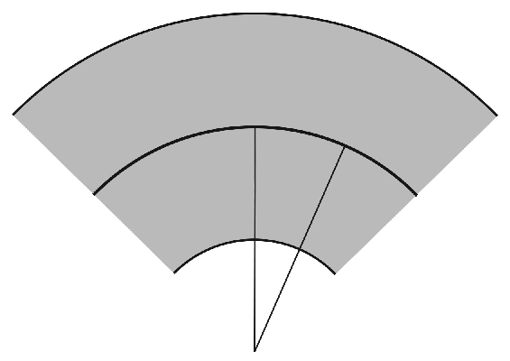
We will derive a rough bound $|{\rm det}\,(\,d_{x}\,{\phi})|\,>\,1/2^{q}$ on the differential of the diffeomorphism ${\phi}\colon\thinspace N_{\epsilon}\longrightarrow{\mathcal{N}}_{\epsilon}$ at any point $x\in N_{\epsilon}$ to get an estimate:

The bound on the differential is particularly easy to see in the case of a hypersurface, pictured in figure 1: due to the choice of ${\epsilon}={\nu}/2$ where ${\nu}$ is the distance to the nearest focal point, the tangent vectors to $S$ do not contract by more than a factor $1/2$ when mapped to any point within ${\mathcal{N}}_{\epsilon}$. (In some directions the tangent vectors expand - however we are looking for just a very rough estimate so we take the “worst case” bound in every direction.) This gives a lower bound of $1/2$ on the eigenvalues of the differential restricted to vectors tangent to $S$, and the vectors tangent to the normal disk are mapped isometrically by $d_{p}\,{\phi}$.

Proving (4.7) in general (for submanifolds of higher codimension) requires a bit more care, and we will refer to [5] for details of the statements below. Fix $p\in S$ and let $u$ be a unit vector normal to $S$ at $p$. Denote by $S_{t}$ the boundary of the tube of radius $t$ around $S$. Then the principal curvatures ${\kappa}_{i},i=1,\ldots,2n-1$ of $S_{t}$ at the point $p+tu$ satisfy the differential equation ${\kappa}^{\prime}_{i}(t)\,=\,({\kappa}_{i}(t))^{2}$ ([5, Corollary 3.5] states this in a more general setting where $R^{2n}$ is replaced with an arbitrary Riemannian manifold.)

The first $q$ of these principal curvatures of $S_{t}$ may be thought of as corresponding to the directions tangent to $S$, and they are given by ${\kappa}_{i}(t)={\kappa}_{i}(0)\,(1-t\,{\kappa}_{i}(0))^{-1}$, $i=1,\ldots,q$. The rest correspond to the directions normal to $S$, ${\kappa}_{i}(t)=-t^{-1}$, $i=q+1,\ldots,2n-1$ (they are equal to the corresponding principal curvatures of the $t$-sphere normal bundle, since the exponential map is an isometry in these directions). Then as expected the determinant of the differential of the exponential map may be expressed in terms of the first $q$ principal curvatures:

see [5, (3.27)]. The principal curvatures ${\kappa}_{i}(0),i=1,\ldots,q$ satisfy the inequality ${\kappa}_{i}(0)\,{\nu}\leq 1$, where as above ${\nu}$ denotes the distance to the nearest focal point [5, section 8.1, Lemma 8.9]. We assumed that $0\leq t\leq{\epsilon}={\nu}/2$, so $1-t{\kappa}_{i}(0)>1/2.$ According to (4.8) then $|{\rm det}\,(\,d_{p}{\phi})|>2^{-q}$, concluding the proof of the estimate (4.7).

We proceed with the proof of theorem 1.4. The complex $K_{l}$ is embedded in the unit ball and the $T$-normal bundles to the simplices are assumed to be embedded. Since ${\nu}$ is the distance to a closest focal point, $T<{\nu}=2{\epsilon}$. If $T>{\epsilon}$ then ${\rm Vol}_{2n}({\mathcal{N}}_{T})\,>\,{\rm Vol}_{2n}({\mathcal{N}}_{\epsilon})$. If $T<{\epsilon}$ then the inequality (4.7) holds for $T$ in place of ${\epsilon}$. In either case, as a consequence of (4.7) one has

where $c_{2n-q}$ is the constant in the expression for the volume of the ball $D^{2n-q}_{T/2}$. The effect of this constant is minor on the final estimate (4.13) on thickness below, so it is omitted in the last term in (4.9). To get a very rough upper bound on ${\rm Vol}({\mathcal{N}}_{T})$ note that the $T$-regular neighborhood of each simplex is embedded in the ball of radius $2$, so its $2n$-volume is less than $(2{\pi})^{n}/n!$. Combine this with the estimate (4.9) where $S$ is largest volume simplex in $i(\bar{S}^{n-1}),i(S^{n}_{2})$ as in (4.6), so ${\rm Vol}_{k}(S)=V^{\prime}_{\alpha}$, respectively $V^{\prime}_{\beta}$:

References

- [1] J. Bourgain, On Lipschitz embedding of finite metric spaces in Hilbert space, Israel J. Math. 52 (1985), 46-52.
- [2] J. Cantarella, R.B. Kusner and J.M. Sullivan, On the minimum ropelength of knots and links, Invent. Math. 150 (2002), 257-286.
- [3] A. Flores, Über -dimensionale Komplexe die im absolut selbstverschlungen sind, Ergeb. math. Koll. 6 (1935), 4-6.
- [4] M. Freedman, V. Krushkal and P. Teichner, Van Kampen’s embedding obstruction is incomplete for 2-complexes in , Math. Res. Lett. 1 (1994), 167-176.
- [5] A. Gray, Tubes, Progress in Mathematics, 221. Birkhäuser Verlag, Basel, 2004.
- [6] M. Gromov, Filling Riemannian manifolds, J. Differential Geom. 18 (1983), 1-147.
- [7] M. Gromov and L. Guth, Generalizations of the Kolmogorov-Barzdin embedding estimates, Duke Math. J. 161 (2012), 2549-2603.
- [8] M. Hastings, with an appendix by M. Freedman, Obstructions To Classically Simulating The Quantum Adiabatic Algorithm, arXiv:1302.5733.
- [9] S. Hoory, N. Linial and A. Wigderson, Expander graphs and their applications, Bull. Amer. Math. Soc. (N.S.) 43 (2006), 439-561.
- [10] A.N. Kolmogorov and Ya.M. Barzdin, On the realization of networks in three-dimensional space, in Selected Works of Kolmogorov, Volume 3, Kluwer Academic Publishers, Dordrecht, 1993.
- [11] N. Linial, E. London, and Yu. Rabinovich, The geometry of graphs and some of its algorithmic applications, Combinatorica 15 (1995), 215-245.
- [12] R.A. Litherland, J. Simon, O. Durumeric, and E. Rawdon, Thickness of knots, Topology Appl. 91 (1999), 233-244.
- [13] G.A. Margulis, Explicit constructions of expanders, Problemy Peredai Informacii 9 (1973), 71-80.
- [14] J. Matoušek, Bi-Lipschitz embeddings into low-dimensional Euclidean spaces, Comment. Math. Univ. Carolin. 31 (1990), 589-600.
- [15] J. Matoušek, On low-distortion embeddings of expanders in , preprint, December 2013.
- [16] J. Matoušek, M. Tancer and U. Wagner, Hardness of embedding simplicial complexes in , J. Eur. Math. Soc. 13 (2011), 259-295.
- [17] S.A. Melikhov, The van Kampen obstruction and its relatives, Proc. Steklov Inst. Math. 266 (2009), no. 1, 142-176.
- [18] J. Milnor, Link groups, Ann. of Math. 59 (1954), 177-195.
- [19] A. Nabutovsky, Non-recursive functions, knots with thick ropes, and self-clenching thick hyperspheres, Comm. Pure Appl. Math. 48 (1995), 381-428.
- [20] M.H.A. Newman, On the division of Euclidean -space by topological - spheres, Proc. Roy. Soc. London Ser. A, 257, 1-12, 1960.
- [21] J. Pardon, On the distortion of knots on embedded surfaces, Ann. of Math. (2) 174 (2011), 637-646.
- [22] A. Shapiro, Obstructions to the imbedding of a complex in a euclidean space. I. The first obstruction, Ann. of Math. 66 (1957), 256-269.
- [23] C. Shonkwiler and D.S. Vela-Vick, Higher-dimensional linking integrals, Proc. Amer. Math. Soc. 139 (2011), 1511-1519.
- [24] J. Stallings, Homology and central series of groups, J. of Algebra 2 (1965), 170-181.
- [25] A. Tarski, A decision method for elementary algebra and geometry. 2nd ed. University of California Press, Berkeley and Los Angeles, Calif., 1951.
- [26] E. R. van Kampen, Komplexe in euklidischen Räumen, Abh. Math. Sem. Univ. Hamburg 9 (1933), 72-78 and 152-153.
- [27] H. Weyl, On the Volume of Tubes, Amer. J. Math. 61 (1939), no. 2, 461-472.