跳到论文正文
W Papers独立论文阅读器 arXiv:1311.2547 论文正文 计算阅读时间 · 0%
引用这篇论文根据当前论文元数据生成,正式投稿前建议核对。


License: arXiv.org perpetual non-exclusive license
arXiv:1311.2547v4 [cs.LG] 30 Jul 2014

Learning Mixtures of Linear Classifiers

Yuekai Sunm1label=e1]yuekai@stanford.edu Email: [    Stratis Ioannidism2label=e2]stratis.ioannidis@technicolor.com Email: [    Andrea Montanarim1label=e3]montanari@stanford.edu Email: [ Affiliation: Stanford University\thanksmarkm1, Technicolor\thanksmarkm2 Address: Institute for Computational and Mathematical Engineering
Stanford University
475 Via Ortega, Stanford, CA 94305
Address:  Address: Technicolor
175 S San Antonio Rd, Los Altos, CA 94022
Address:  Address: Department of Electrical Engineering
Department of Statistics
Stanford University
350 Serra Mall, Stanford, CA 94305
Address: 
Abstract

We consider a discriminative learning (regression) problem, whereby the regression function is a convex combination of kk linear classifiers. Existing approaches are based on the EM algorithm, or similar techniques, without provable guarantees. We develop a simple method based on spectral techniques and a ‘mirroring’ trick, that discovers the subspace spanned by the classifiers’ parameter vectors. Under a probabilistic assumption on the feature vector distribution, we prove that this approach has nearly optimal statistical efficiency.

††email: e1††email: e2††email: e3
\setattribute

journalname

, and

1 Introduction

Since Pearson’s seminal contribution (Pearson, 1894), and most notably after the introduction of the EM algorithm (Dempster, Laird and Rubin, 1977), mixture models and latent variable models have played a central role in statistics and machine learning, with numerous applications—see, e.g., McLachlan and Peel (2004), Bishop (1998), and Bartholomew, Knott and Moustaki (2011). Despite their ubiquity, fitting the parameters of a mixture model remains a challenging task. The most popular methods (e.g., the EM algorithm or likelihood maximization by gradient ascent) are plagued by local optima and come with little or no guarantees. Computationally efficient algorithms with provable guarantees are an exception in this area. Even the idealized problem of learning mixtures of Gaussians has motivated a copious theoretical literature (Arora and Kannan, 2001; Moitra and Valiant, 2010).

In this paper we consider the problem of modeling a regression function as a mixture of kk components. Namely, we are given labels Yi∈ℝY_{i}\in\mathbb{R} and feature vectors Xi∈ℝdX_{i}\in\mathbb{R}^{d}, i∈[n]≡{1,2,…,n}i\in[n]\equiv\{1,2,\dots,n\}, and we seek estimates of the parameters of a mixture model

Yi|Xi=xi∼∑ℓ=1kpℓ​f​(yi|xi,uℓ).\displaystyle Y_{i}\big|_{X_{i}=x_{i}}\sim\textstyle\sum_{\ell=1}^{k}p_{\ell}\,f(y_{i}|x_{i},u_{\ell})\,. (1)

Here kk is the number of components, (pℓ)ℓ∈[k](p_{\ell})_{\ell\in[k]} are weights of the components, and uℓu_{\ell} is a vector of parameters for the ℓ\ell-th component. Models of this type have been intensely studied in the neural network literature since the early nineties (Jordan and Jacobs, 1994; Bishop, 1998). They have also found numerous applications ranging from object recognition (Quattoni, Collins and Darrell, 2004) to machine translation (Liang et al., 2006). These studies are largely based on learning algorithms without consistency guarantees.

Recently, Chaganty and Liang (2013) considered mixtures of linear regressions, whereby the relation between labels and feature vectors is linear within each component; i.e., Yi=⟨uℓ,Xi⟩+noiseY_{i}=\langle u_{\ell},X_{i}\rangle+{\rm noise} (here and below ⟨a,b⟩\langle a,b\rangle denotes the standard inner product in ℝm\mathbb{R}^{m}). Equivalently, f⁡(yi|xi,uℓ)=f0​(yi−⟨xi,uℓ⟩)f(y_{i}|x_{i},u_{\ell})=f_{0}(y_{i}-\langle x_{i},u_{\ell}\rangle) with f0​(⋅)f_{0}(\,\cdot\,) a density of mean zero. Building on a new approach developed by Hsu, Kakade and Zhang (2012) and Anandkumar et al. (2012), these authors propose an algorithm for fitting mixtures of linear regressions with provable guarantees. The main idea is to regress YiqY_{i}^{q}, for q∈{1,2,3}q\in\{1,2,3\} against the tensors XiX_{i}, Xi⊗XiX_{i}\otimes X_{i}, Xi⊗Xi⊗XiX_{i}\otimes X_{i}\otimes X_{i}. The coefficients of these regressions are tensors whose decomposition yields the parameters uℓu_{\ell}, pℓp_{\ell}.

While the work of Chaganty and Liang (2013) is a significant step forward, it leaves several open problems:

Statistical efficiency. Consider a standard scaling of the feature vectors, whereby the components (Xi,j)j∈[p](X_{i,j})_{j\in[p]} are of order one. Then, the mathematical guarantees of Chaganty and Liang (2013) require a sample size n≫d6n\gg d^{6}. This is substantially larger than the ‘information-theoretic’ optimal scaling, and is an unrealistic requirement in high-dimension (large dd). As noted in (Chaganty and Liang, 2013), this scaling is an intrinsic drawback of the tensor approach as it operates in a higher-dimensional space (tensor space) than the space in which data naturally live.

Linear regression versus classification. In virtually all applications of the mixture model (1), labels YiY_{i} are categorical—see, e.g., Jordan and Jacobs (1994), Bishop (1998), Quattoni, Collins and Darrell (2004), Liang et al. (2006). In this case, the very first step of Chaganty & Liang, namely, regressing Yi2Y_{i}^{2} on Xi⊗2X_{i}^{\otimes 2} and Yi3Y_{i}^{3} on Xi⊗3X_{i}^{\otimes 3}, breaks down. Consider—to be definite—the important case of binary labels (e.g., Yi∈{0,1}Y_{i}\in\{0,1\} or Yi∈{+1,−1}Y_{i}\in\{+1,-1\}). Then powers of the labels do not provide additional information (e.g., if Yi∈{0,1}Y_{i}\in\{0,1\}, then Yi=Yi2Y_{i}=Y_{i}^{2}). Also, since YiY_{i} is non-linearly related to uℓu_{\ell}, Yi2Y_{i}^{2} does not depend only on uℓ⊗2u_{\ell}^{\otimes 2}.

Computational complexity. The method of Chaganty and Liang (2013) solves a regularized linear regression in d3d^{3} dimensions and factorizes a third order tensor in dd dimensions. Even under optimistic assumptions (finite convergence of iterative schemes), this requires O⁡(d3​n+d4)O(d^{3}n+d^{4}) operations.

In this paper, we develop a spectral approach to learning mixtures of linear classifiers in high dimension. For the sake of simplicity, we shall focus on the case of binary labels Yi∈{+1,−1}Y_{i}\in\{+1,-1\}, but we expect our ideas to be more broadly applicable. We consider regression functions of the form f⁡(yi|xi,uℓ)=f⁡(yi|⟨xi,uℓ⟩)f(y_{i}|x_{i},u_{\ell})=f(y_{i}|\langle x_{i},u_{\ell}\rangle), i.e., each component corresponds to a generalized linear model with parameter vector uℓ∈ℝdu_{\ell}\in\mathbb{R}^{d}. In a nutshell, our method constructs a symmetric matrix Q^∈ℝd×d\hat{Q}\in\mathbb{R}^{d\times d} by taking a suitable empirical average of the data. The matrix Q^\hat{Q} has the following property: (d−k)(d-k) of its eigenvalues are roughly degenerate. The remaining kk eigenvalues correspond to eigenvectors that—approximately—span the same subspace as u1u_{1}, …, uku_{k}. Once this space is accurately estimated, the problem dimensionality is reduced to kk; as such, it is easy to come up with effective prediction methods (as a matter of fact, simple KK-nearest neighbors works very well).

The resulting algorithm is computationally efficient, as its most expensive step is computing the eigenvector decomposition of a d×dd\times d matrix (which takes O⁡(d3)O(d^{3}) operations). Assuming Gaussian feature vectors Xi∈ℝdX_{i}\in\mathbb{R}^{d}, we prove that our method is also statistically efficient, i.e., it only requires n≥dn\geq d samples to accurately reconstruct the subspace spanned by u1,…,uku_{1},\dots,u_{k}. This is the same amount of data needed to estimate the covariance of the feature vectors XiX_{i} or a parameter vector u1∈ℝdu_{1}\in\mathbb{R}^{d} in the trivial case of a mixture with a single component, k=1k=1. It is unlikely that a significantly better efficiency can be achieved without additional structure.

The assumption of Gaussian feature vectors XiX_{i}’s is admittedly restrictive. On one hand, as for the problem of learning mixtures of Gaussians (Arora and Kannan, 2001; Moitra and Valiant, 2010), we believe that useful insights can be gained by studying this simple setting. On the other, and as discussed below, our proof does not really require the distribution of the XiX_{i}’s to be Gaussian, and a strictly weaker assumption is sufficient. We expect that future work will succeed in further relaxing this assumption.

1.1 Technical contribution and related work

Our approach is related to the principal Hessian directions (pHd) method proposed by Li (1992) and further developed by Cook (1998) and co-workers. PHd is an approach to dimensionality reduction and data visualization. It generalizes principal component analysis to the regression (discriminative) setting, whereby each data point consists of a feature vector Xi∈ℝdX_{i}\in\mathbb{R}^{d} and a label Yi∈ℝY_{i}\in\mathbb{R}. Summarizing, the idea is to form the ‘Hessian’ matrix H^=n−1​∑i=1nYi​Xi​XiT∈ℝd×d\hat{H}=n^{-1}\sum_{i=1}^{n}Y_{i}\,X_{i}X_{i}^{T}\in\mathbb{R}^{d\times d}. (We assume here, for ease of exposition, that the XiX_{i}’s have zero mean and unit covariance.) The eigenvectors associated to eigenvalues with largest magnitude are used to identify a subspace in ℝd\mathbb{R}^{d} onto which to project the feature vectors XiX_{i}’s.

Unfortunately, the pHd approach fails in general for the mixture models of interest here, namely, mixtures of linear classifiers. For instance, it fails when each component of (1) is described by a logistic model f⁡(yi=+1|z)=(1+e−z)−1f(y_{i}=+1|z)=(1+e^{-z})^{-1}, when features are centered at 𝔼⁡(Xi)=0{\mathbb{E}}(X_{i})=0; a proof can be found in Appendix D.

Our approach overcomes this problem by constructing Q^=n−1​∑i=1nZi​Xi​XiT∈ℝd×d\hat{Q}=n^{-1}\sum_{i=1}^{n}Z_{i}\,X_{i}X_{i}^{T}\in\mathbb{R}^{d\times d}. The ZiZ_{i}’s are pseudo-labels obtained by applying a ‘mirroring’ transformation to the YiY_{i}’s. Unlike with H^\hat{H}, the eigenvector structure of Q^\hat{Q} enables us to estimate the span of u1,…,uku_{1},\dots,u_{k}.

As an additional technical contribution, we establish non-asymptotic bounds on the estimation error that allow to characterize the trade-off between the data dimension dd and the sample size nn. In contrast, rigorous analysis on pHd is limited to the low-dimensional regime of dd fixed as n→∞n\to\infty. It would be interesting to generalize the analysis developed here to characterize the high-dimensional properties of pHd as well.

2 Problem Formulation

Refer to caption
Refer to caption
Refer to caption

(a) (b) (c)

Figure 1: The mirroring process applied to a mixture of two 3-dimensional classifiers. Figure (a) shows labels generated by two classifiers in ℝ3\mathbb{R}^{3}; the figure includes the parameter profiles as well as the corresponding classification surfaces. Figure (b) shows the mirroring direction r^\hat{r} as a dashed vector, computed by (5), as well as the plane it defines; note that r^\hat{r} lies within the positive cone spanned by the two classifier profiles, approximately. Finally, Figure (c) shows the result of the mirroring process: the region of points that was predominantly positive has remained unaltered, while the region of points that was predominantly negative has been flipped.

2.1 Model

Consider a dataset comprising nn i.i.d. pairs (Xi,Yi)∈ℝd×{−1,+1}(X_{i},Y_{i})\in\mathbb{R}^{d}\times\{-1,+1\}, i∈[n]i\in[n]. We refer to the vectors Xi∈ℝdX_{i}\in\mathbb{R}^{d} as features and to the binary variables as labels. We assume that the features Xi∈ℝdX_{i}\in\mathbb{R}^{d} are sampled from a Gaussian distribution with mean μ∈ℝd\mu\in\mathbb{R}^{d} and a positive definite covariance Σ∈ℝd×d\Sigma\in\mathbb{R}^{d\times d}. The labels Yi∈{−1,+1}Y_{i}\in\{-1,+1\} are generated by a mixture of linear classifiers, i.e.,

𝐏𝐫⁡(Yi=+1∣Xi)=∑ℓ=1kpℓ​f​(⟨uℓ,Xi⟩).\displaystyle\mathbf{Pr}(Y_{i}=+1\mid X_{i})=\textstyle\sum_{\ell=1}^{k}p_{\ell}\,f(\langle u_{\ell},X_{i}\rangle)\,. (2)

Here, k≥2k\geq 2 is the number of components in the mixture; (pℓ)ℓ∈[k](p_{\ell})_{\ell\in[k]} are the weights, satisfying of course pℓ>0p_{\ell}>0, ∑ℓ=1kpℓ=1\sum_{\ell=1}^{k}p_{\ell}=1; and (uℓ)ℓ∈[k](u_{\ell})_{\ell\in[k]}, uℓ∈ℝdu_{\ell}\in\mathbb{R}^{d} are the normals to the planes defining the kk linear classifiers. We refer to each normal uℓu_{\ell} as the parameter profile of the ℓ\ell-th classifier; we assume that the profiles uℓu_{\ell}, ℓ∈[k]\ell\in[k], are linearly independent, and that k<n/2k<n/2.

We assume that the function f:ℝ→[0,1]f:\mathbb{R}\to[0,1], characterizing the classifier response, is analytic, non-decreasing, strictly concave in [0,+∞)[0,+\infty), and satisfies:

limt→∞f⁡(t)=1,limt→−∞f⁡(t)=0,−f⁡(t)=f⁡(−t).\displaystyle\lim_{t\to\infty}\!f(t)\!=\!1,~~\lim_{t\to-\infty}\!f(t)\!=\!0,\quad 1\!-\!f(t)\!=\!f(-t). (3)

As an example, it is useful to keep in mind the logistic function f⁡(t)=(1+e−t)−1f(t)=(1+e^{-t})^{-1}. Fig. 1(a) illustrates a mixture of k=2k=2 classifiers over d=3d=3 dimensions.

2.2 Subspace Estimation, Prediction and Clustering

Our main focus is the following task:

Subspace Estimation: After observing (Xi,Yi),(X_{i},Y_{i}), i∈[n]i\in[n], estimate the subspace spanned by the profiles of the kk classifiers, i.e., U≡span⁡(u1,…,uk)U\equiv{\rm span}(u_{1},\dots,u_{k}).

For U^\widehat{U} an estimate of UU, we characterize performance via the principal angle between the two spaces, namely

dP​(U,U^)=maxx∈U,y∈U^⁡arccos⁡(⟨x,y⟩‖x‖​‖y‖).d_{P}(U,\widehat{U})=\max_{x\in U,y\in\widehat{U}}\arccos\left(\tfrac{\langle x,y\rangle}{\|x\|\|y\|}\right).

Notice that projecting the features XiX_{i} on UU entails no loss of information w.r.t. (2). This can be exploited to improve the performance of several learning tasks through dimensionality reduction, by projecting the features to the estimate of the subspace UU. Two such tasks are:

Prediction: Given a new feature vector Xn+1X_{n+1}, predict the corresponding label Yn+1Y_{n+1}.

Clustering: Given a new feature vector and label pair (Xn+1,Yn+1)(X_{n+1},Y_{n+1}), identify the classifier that generated the label.

As we will see in Section 5, our subspace estimate can be used to significantly improve the performance of both prediction and clustering.

2.3 Technical Preliminary

We review here a few definitions used in our exposition. The sub-gaussian norm of a random variable XX is:

‖X‖ψ2=supp≥11p​(𝔼⁡[|X|p])1/p.\|X\|_{\psi_{2}}=\sup_{p\geq 1}\frac{1}{\sqrt{p}}(\mathbb{E}[|X|^{p}])^{1/p}.

We say XX is sub-gaussian if ‖X‖ψ2<∞\|X\|_{\psi_{2}}<\infty. We say that a random vector X∈ℝdX\in\mathbb{R}^{d} is sub-gaussian if ⟨y,X⟩\langle y,X\rangle is sub-gaussian for any yy on the unit sphere 𝐒d−1\mathbf{S}^{d-1}.

We use the following variant of Stein’s identity Stein (1973); Liu (1994). Let X∈ℝdX\in\mathbb{R}^{d}, X′∈ℝd′X^{\prime}\in\mathbb{R}^{d^{\prime}} be jointly Gaussian random vectors, and consider a function h:ℝd′→ℝh:\mathbb{R}^{d^{\prime}}\to\mathbb{R} that is almost everywhere (a.e.) differentiable and satisfies 𝔼⁡[|∂h⁡(X′)/∂xi|]<∞\mathbb{E}[|\partial h(X^{\prime})/\partial x_{i}|]<\infty, i∈[d′]i\in[d^{\prime}]. Then, the following identity holds:

Cov⁡(X,h⁡(X′))=Cov⁡(X,X′)​𝔼​[∇h​(X′)].\displaystyle\mathrm{Cov}(X,h(X^{\prime}))=\mathrm{Cov}(X,X^{\prime})\mathbb{E}[\nabla h(X^{\prime})]. (4)

3 Subspace Estimation

Algorithm 1 SpectralMirror
0:  Pairs (Xi,Yi)(X_{i},Y_{i}), i∈[n]i\in[n]
0:  Subspace estimate U^\widehat{U}
1:  μ^←1⌊n/2⌋​∑i=1⌊n/2⌋Xi\hat{\mu}\leftarrow\frac{1}{\lfloor n/2\rfloor}\sum_{i=1}^{\lfloor n/2\rfloor}X_{i}
2:  Σ^←1⌈n/2⌉​∑i=1⌊n/2⌋(Xi−μ^)​(Xi−μ^)T\hat{\Sigma}\leftarrow\frac{1}{\lceil n/2\rceil}\sum_{i=1}^{\lfloor n/2\rfloor}(X_{i}-\hat{\mu})(X_{i}-\hat{\mu})^{T}
3:  r^←1⌊n/2⌋​∑i=1⌊n/2⌋Yi​Σ^−1​(Xi−μ^)\hat{r}\leftarrow\frac{1}{\lfloor n/2\rfloor}\sum_{i=1}^{\lfloor n/2\rfloor}Y_{i}\hat{\Sigma}^{-1}(X_{i}\!-\!\hat{\mu})
4:   for each i∈{⌊n/2⌋+1,…,n}i\in\{\lfloor n/2\rfloor+1,\dots,n\}:
Zi←Yi​sgn⟨r^,Xi⟩Z_{i}\leftarrow Y_{i}\mathop{\mathrm{sgn}}\langle\hat{r},X_{i}\rangle\vskip-17.07182pt
5:   Q^←1⌈n/2⌉∑i=⌊n/2⌋+1nZiΣ^−1/2(Xi−μ^)(Xi−μ^)TΣ^−1/2\displaystyle\hat{Q}\!\!\leftarrow\!\!\frac{1}{\lceil n/2\rceil}\!\!\sum_{i=\lfloor n/2\rfloor+1}^{n}\!\!\!\!\!Z_{i}\hat{\Sigma}^{-1/2}(X_{i}\!-\!\hat{\mu})(X_{i}\!-\!\hat{\mu})^{T}\hat{\Sigma}^{-1/2}
6:  Find eigendecomposition ∑ℓ=1dλℓ​wℓ​wℓT\sum_{\ell=1}^{d}\lambda_{\ell}w_{\ell}w_{\ell}^{T} of Q^\hat{Q}
7:  Let λ(1),…,λ(k)\lambda_{(1)},\ldots,\lambda_{(k)} be the kk eigenvalues furthest from the median.
8:  U^←span(Σ^−1/2w(1),…,Σ^−1/2w(k))\hat{U}\leftarrow\linspan\left(\hat{\Sigma}^{-1/2}w_{(1)},\ldots,\hat{\Sigma}^{-1/2}w_{(k)}\right)

In this section, we present our algorithm for subspace estimation, which we refer to as SpectralMirror. Our main technical contribution, stated formally below, is that the output U^\hat{U} of SpectralMirror is a consistent estimator of the subspace UU as soon as n≥C​dn\geq C\,d, for a sufficiently large constant CC.

3.1 Spectral Mirror Algorithm

We begin by presenting our algorithm for estimating the subspace span UU. Our algorithm consists of three main steps. First, as pre-processing, we estimate the mean and covariance of the underlying features XiX_{i}. Second, using these estimates, we identify a vector r^\hat{r} that concentrates near the convex cone spanned by the profiles (uℓ)ℓ∈[k](u_{\ell})_{\ell\in[k]}. We use this vector to perform an operation we call mirroring: we ‘flip’ all labels lying in the negative halfspace determined by r^\hat{r}. Finally, we compute a weighted covariance matrix Q^\hat{Q} over all XiX_{i}, where each point’s contribution is weighed by the mirrored labels: the eigenvectors of this matrix, appropriately transformed, yield the span UU.

These operations are summarized in Algorithm 1. We discuss each of the main steps in more detail below:

Pre-processing. (Lines 1–2) We split the dataset into two halves. Using the first half (i.e., all XiX_{i} with OPEN1≤i≤⌊n2⌋)1\leq i\leq\lfloor\frac{n}{2}\rfloor), we construct estimates μ^∈ℝd\hat{\mu}\in\mathbb{R}^{d} and Σ^∈ℝd×d\hat{\Sigma}\in\mathbb{R}^{d\times d} of the feature mean and covariance, respectively. Standard Gaussian (i.e., ‘whitened’) versions of features XiX_{i} can be constructed as Σ^−1/2(Xi−μ^)\hat{\Sigma}^{-1/2}(X_{i}\!-\!\hat{\mu}).

Mirroring. (Lines 3–4) We compute the vector:

r^=1⌊n/2⌋​∑i=1⌊n/2⌋Yi​Σ^−1​(Xi−μ^)∈ℝd.\displaystyle\hat{r}=\frac{1}{\lfloor n/2\rfloor}\textstyle\sum_{i=1}^{\lfloor n/2\rfloor}Y_{i}\hat{\Sigma}^{-1}(X_{i}\!-\!\hat{\mu})\in\mathbb{R}^{d}. (5)

We refer to r^\hat{r} as the mirroring direction. In Section 4, we show that r^\hat{r} concentrates around its population (n=∞n=\infty) version r≡𝔼⁡[Y​Σ−1​(X−μ)]r\equiv\mathbb{E}[Y\Sigma^{-1}(X-\mu)]. Crucially, rr lies in the interior of the convex cone spanned by the parameter profiles, i.e., r=∑ℓ=1kαℓ​uℓr=\sum_{\ell=1}^{k}\alpha_{\ell}u_{\ell}, for some positive αℓ>0\alpha_{\ell}>0, ℓ∈[k]\ell\in[k] (see Lemma 2 and Fig. 1(b)). Using this r^\hat{r}, we ‘mirror’ the labels in the second part of the dataset:

Zi=Yi​sgn⟨r^,Xi⟩,for ​⌊n/2⌋<i≤n.Z_{i}=Y_{i}\mathop{\mathrm{sgn}}\langle\hat{r},X_{i}\rangle,\quad\text{for~}\lfloor n/2\rfloor<i\leq n.

In words, ZiZ_{i} equals YiY_{i} for all ii in the positive half-space defined by the mirroring direction; instead, all labels for points ii in the negative half-space are flipped (i.e., Zi=−YiZ_{i}=-Y_{i}). This is illustrated in Figure 1(c).

Spectral Decomposition. (Lines 5–8) The mirrored labels are used to compute a weighted covariance matrix over whitened features as follows:

Q^\displaystyle\hat{Q} =1⌈n2⌉∑i=⌊n/2⌋+1nZiΣ^−1/2(Xi−μ^)(Xi−μ^)TΣ^−1/2\displaystyle=\frac{1}{\lceil\frac{n}{2}\rceil}\sum_{i=\lfloor n/2\rfloor+1}^{n}Z_{i}\hat{\Sigma}^{-1/2}(X_{i}-\hat{\mu})(X_{i}-\hat{\mu})^{T}\hat{\Sigma}^{-1/2}

The spectrum of Q^\hat{Q} has a specific structure, that reveals the span UU. In particular, as we will see in Section 4, Q^\hat{Q} converges to a matrix QQ that contains an eigenvalue with multiplicity n−kn-k; crucially, the eigenvectors corresponding to the remaining kk eigenvalues, subject to the linear transform Σ^−1/2\hat{\Sigma}^{-1/2}, span the subspace UU. As such, the final steps of the algorithm amount to discovering the eigenvalues that ‘stand out’ (i.e., are different from the eigenvalue with multiplicity n−kn-k), and rotating the corresponding eigenvectors to obtain U^\hat{U}. More specifically, let (λℓ,wℓ)ℓ∈[d](\lambda_{\ell},w_{\ell})_{\ell\in[d]} be the eigenvalues and eigenvectors of Q^\hat{Q}. Recall that k<n/2k<n/2. The algorithm computes the median of all eigenvalues, and identifies the kk eigenvalues furthest from this median; these are the ‘outliers’. The corresponding kk eigenvectors, multiplied by Σ^−1/2\hat{\Sigma}^{-1/2}, yield the subspace estimate U^\hat{U}.

The algorithm does not require knowledge of the classifier response function ff. Also, while we assume knowledge of kk, an eigenvalue/eigenvectors statistic (see, e.g., Zelnik-Manor and Perona (2004)) can be used to estimate kk, as the number of ‘outlier’ eigenvalues.

3.2 Main Result

Our main result states that SpectralMirror is a consistent estimator of the subspace spanned by (uℓ)ℓ∈[k](u_{\ell})_{\ell\in[k]}. This is true for ‘most’ μ∈ℝd\mu\in\mathbb{R}^{d}. Formally, we say that an event occurs for generic μ\mu if adding an arbitrarily small random perturbation to μ\mu, the event occurs with probability 11 w.r.t. this perturbation.

Theorem 1.

Denote by U^\hat{U} the output of SpectralMirror, and let Pr⊥≡I−r​rT/‖r‖2P^{\bot}_{r}\equiv I-rr^{T}/\|r\|^{2} be the projector orthogonal to rr, given by (6). Then, for generic μ\mu, as well as for μ=0\mu=0, there exists ϵ0>0\epsilon_{0}>0 such that, for all ϵ∈[0,ϵ0)\epsilon\in[0,\epsilon_{0}),

𝐏𝐫⁡(dP​(Pr⊥​U,U^)>ϵ)≤C1​exp⁡(−C2​n​ϵ2d).\displaystyle\mathbf{Pr}(d_{P}(P^{\bot}_{r}U,\hat{U})>\epsilon)\leq C_{1}\exp(-C_{2}\frac{n\epsilon^{2}}{d}).

Here C1C_{1} is an absolute constant, and C2>0C_{2}>0 depends on μ\mu, Σ\Sigma, ff and (uℓ)ℓ∈[k](u_{\ell})_{\ell\in[k]}.

In other words, U^\hat{U} provides an accurate estimate of Pr⊥​UP^{\bot}_{r}U as soon as nn is significantly larger than dd. This holds for generic μ\mu, but we also prove that it holds for the specific and important case where μ=0\mu=0; in fact, it also holds for all small-enough μ\mu. Note that this does not guarantee that U^\hat{U} spans the direction r∈Ur\in U; nevertheless, as shown below, the latter is accurately estimated by r^\hat{r} (see Lemma 1) and can be added to the span, if necessary. Moreover, our experiments suggest this is rarely the case in practice, as U^\hat{U} indeed includes the direction rr (see Section 5).

4 Proof of Theorem 1

Recall that we denote by rr the population (n=∞n=\infty) version of r^\hat{r}. Let g⁡(s)≡2​f​(s)−1g(s)\equiv 2f(s)-1, for s∈ℝs\in\mathbb{R}, and observe that 𝔼⁡[Y∣X=x]=∑ℓ=1kpℓ​g​(⟨uℓ,x⟩).\mathbb{E}[Y\mid X=x]=\sum_{\ell=1}^{k}p_{\ell}g(\langle u_{\ell},x\rangle). Hence,

r=𝔼⁡[Σ−1​(X−μ)⋅(∑ℓ=1kpℓ​g​(⟨uℓ,X⟩))].\displaystyle r=\mathbb{E}\left[\Sigma^{-1}(X-\mu)\cdot\left(\textstyle\sum_{\ell=1}^{k}p_{\ell}g(\langle u_{\ell},X\rangle)\right)\right]. (6)

Then, the following concentration result holds:

Lemma 1.

There exist an absolute constant C>0C>0 and c1,c1′,c2′c_{1},c_{1}^{\prime},c_{2}^{\prime} that depend on ‖X‖ψ2\|X\|_{\psi_{2}} such that:

𝐏𝐫⁡(‖r^−r‖2≥ϵ)≤C​e−min⁡{c2​n​ϵ2d,(c1′​n​ϵ−c2′​d)2}.\mathbf{Pr}(\|\hat{r}-r\|_{2}\!\geq\!\epsilon)\!\leq\!Ce^{-\min\bigl\{\frac{c_{2}n\epsilon^{2}}{d},\bigl(c_{1}^{\prime}\sqrt{n}\epsilon-c_{2}^{\prime}\sqrt{d}\bigr)^{2}\bigr\}}.

The proof of Lemma 1 relies on a large deviation inequality for sub-Gaussian vectors, and is provided in Appendix B. Crucially, rr lies in the interior of the convex cone spanned by the parameter profiles:

Lemma 2.

r=∑ℓ=1kαℓ​uℓr=\sum_{\ell=1}^{k}\alpha_{\ell}u_{\ell} for some αℓ>0\alpha_{\ell}>0, ℓ∈[k]\ell\in[k].

Proof.

From (6),

r=∑ℓ=1kpℓ​Σ−1​𝔼​[(X−μ)​g​(⟨uℓ,X⟩)].\textstyle r=\sum_{\ell=1}^{k}p_{\ell}\Sigma^{-1}\mathbb{E}[(X-\mu)g(\langle u_{\ell},X\rangle)].

It thus suffices to show that Σ−1​𝔼​[(X−μ)​g​(⟨u,X⟩)]=α​u\Sigma^{-1}\mathbb{E}[(X-\mu)g(\langle u,X\rangle)]=\alpha u, for some α>0\alpha>0. Note that X′=⟨u,X⟩X^{\prime}=\langle u,X\rangle is normal with mean μ0=uT​μ\mu_{0}=u^{T}\mu and variance σ02=uT​Σ​u>0\sigma_{0}^{2}=u^{T}\Sigma u>0. Since ff is analytic and non-decreasing, so is gg; moreover, g′≥0g^{\prime}\geq 0. This, and the fact that gg is non-constant, implies 𝔼⁡[g′​(X′)]>0\mathbb{E}[g^{\prime}(X^{\prime})]>0. On the other hand, from Stein’s identity (4), 𝔼⁡[g′​(X′)]=1σ02​𝔼​[X′​g​(X′)]<∞\mathbb{E}[g^{\prime}(X^{\prime})]=\frac{1}{\sigma_{0}^{2}}\mathbb{E}[X^{\prime}g(X^{\prime})]<\infty, as gg is bounded. Hence:

Σ−1​𝔼​[(X−μ)​g​(⟨u,X⟩)]\displaystyle\Sigma^{-1}\mathbb{E}[(X-\mu)g(\langle u,X\rangle)]
=(4)Σ−1​Cov​(X,⟨u,X⟩)​𝔼​[g′​(X′)],where​X′∼𝒩⁡(μ0,σ02)\displaystyle\stackrel{{\scriptstyle\eqref{stein}}}{{=}}\Sigma^{-1}\mathrm{Cov}(X,\langle u,X\rangle)\mathbb{E}[g^{\prime}(X^{\prime})],~\text{where}~X^{\prime}\sim\mathcal{N}(\mu_{0},\sigma_{0}^{2})
=Σ−1⋅𝔼⁡[(X−μ)​XT​u]⋅𝔼⁡[g′​(X′)]\displaystyle=\Sigma^{-1}\cdot\mathbb{E}[(X-\mu)X^{T}u]\cdot\mathbb{E}[g^{\prime}(X^{\prime})]
=Σ−1⋅Σ​u⋅𝔼⁡[g′​(X′)]=𝔼⁡[g′​(X′)]⋅u\displaystyle=\Sigma^{-1}\cdot\Sigma u\cdot\mathbb{E}[g^{\prime}(X^{\prime})]=\mathbb{E}[g^{\prime}(X^{\prime})]\cdot u

and the lemma follows. ∎

For rr and (αℓ)ℓ∈[k](\alpha_{\ell})_{\ell\in[k]} as in Lemma 2, define

z⁡(x)\displaystyle z(x) =𝔼⁡[Y​sgn(⟨r,X⟩)∣X=x]\displaystyle=\mathbb{E}[Y\mathop{\mathrm{sgn}}(\langle r,X\rangle)\mid X=x]
=(∑ℓ=1kpℓ​g​(⟨x,uℓ⟩))⋅sgn(∑ℓ=1kαℓ​⟨x,uℓ⟩).\displaystyle=\textstyle\left(\sum_{\ell=1}^{k}p_{\ell}g(\langle x,u_{\ell}\rangle)\right)\cdot\mathop{\mathrm{sgn}}\left(\sum_{\ell=1}^{k}\alpha_{\ell}\langle x,u_{\ell}\rangle\right).

Observe that z⁡(x)z(x) is the expectation of the mirrored label at a point xx presuming that the mirroring direction is exactly rr. Let Q∈ℝd×dQ\in\mathbb{R}^{d\times d} be the matrix:

Q=𝔼[z(X)Σ−1/2(X−μ)(X−μ)TΣ−1/2].Q=\mathbb{E}[z(X)\Sigma^{-1/2}(X-\mu)(X-\mu)^{T}\Sigma^{-1/2}].

Then Q^\hat{Q} concentrates around QQ, as stated below.

Lemma 3.

Let ϵ0≡min⁡{α1,…,αk}​σmin​(U)\epsilon_{0}\equiv\min\{\alpha_{1},\dots,\alpha_{k}\}\sigma_{\min}(U), where the αℓ>0\alpha_{\ell}>0 are defined as per Lemma 2 and σmin​(U)\sigma_{\min}(U) is the smallest non-zero singular value of UU. Then for ϵ<min⁡(ϵ0,‖r‖/2)\epsilon<\min(\epsilon_{0},\|r\|/2):

𝐏𝐫⁡(‖Q^−Q‖2>ϵ)≤C​exp⁡{−F⁡(ϵ2)},\mathbf{Pr}(\|\hat{Q}-Q\|_{2}>\epsilon)\leq C\exp\{-F(\epsilon^{2})\},

where F⁡(ϵ)≡min⁡{c1​n​ϵ2d,(c1′​n​ϵ−c2′​d)2},F(\epsilon)\equiv\min\left\{\frac{c_{1}n\epsilon^{2}}{d},\bigl(c_{1}^{\prime}\sqrt{n}\epsilon-c_{2}^{\prime}\sqrt{d}\bigr)^{2}\right\}, CC an absolute constant, and c1,c1′,c2′c_{1},\,c_{1}^{\prime},\,c_{2}^{\prime} depend on μ\mu, Σ\Sigma, and ‖r‖\|r\|.

The proof of Lemma 3 is in Appendix C. We again rely on large deviation bounds for sub-gaussian random variables; nevertheless, our proof diverges from standard arguments because r^\hat{r}, rather than rr, is used as a mirroring direction. Additional care is needed to ensure that (a) when r^\hat{r} is close enough to rr, its projection to UU lies in the interior of the convex cone spanned by the profiles, and (b) although r^\hat{r} may have a (vanishing) component outside the convex cone, the effect this has on Q^\hat{Q} is negligible, for nn large enough.

An immediate consequence of Lemma 2 is that rr reveals a direction in the span UU. The following lemma states that the eigenvectors of QQ, subject to a rotation, yield the remaining k−1k-1 directions:

Lemma 4.

Matrix QQ has at most k+1k+1 distinct eigenvalues. One eigenvalue, termed λ0\lambda_{0}, has multiplicity d−kd-k. For generic μ\mu, as well as for μ=0\mu=0, the eigenvectors w1,…,wkw_{1},\ldots,w_{k} corresponding to the remaining eigenvalues λ1\lambda_{1}, …, λk\lambda_{k} are such that

Pr⊥U=span(Pr⊥Σ−1/2w1,…,Pr⊥Σ−1/2wk),P^{\bot}_{r}U=\linspan(P^{\bot}_{r}\Sigma^{-1/2}w_{1},\ldots,P^{\bot}_{r}\Sigma^{-1/2}w_{k}),

where Pr⊥P^{\bot}_{r} is the projection orthogonal to rr.

Proof.

Note that

Q\displaystyle Q =𝔼⁡[z⁡(X)​Σ−12​(X−μ)​(X−μ)T​Σ−12]\displaystyle=\mathbb{E}[z(X)\Sigma^{-\frac{1}{2}}(X-\mu)(X-\mu)^{T}\Sigma^{-\frac{1}{2}}]
=𝔼⁡[z⁡(Σ1/2​W+μ)​W​WT],where ​W∼𝒩⁡(0,I)\displaystyle=\mathbb{E}[z(\Sigma^{1/2}W+\mu)WW^{T}],\quad\text{where }W\sim\mathcal{N}(0,I)
=𝔼⁡[∑ℓ=1kpℓ​g​(⟨Σ12​W+μ,uℓ⟩)​sgn(⟨Σ12​W+μ,r⟩)​W​WT]\displaystyle=\mathbb{E}\big[\sum_{\ell=1}^{k}p_{\ell}g(\langle\Sigma^{\frac{1}{2}}W\!+\!\mu,\!u_{\ell}\rangle)\mathop{\mathrm{sgn}}(\langle\Sigma^{\frac{1}{2}}W\!+\!\mu,\!r\rangle)WW^{T}\big]
=𝔼⁡[∑ℓ=1kpℓ​g​(⟨W+μ~,u~ℓ⟩)​sgn(⟨W+μ~,r~⟩)​W​WT]\displaystyle=\mathbb{E}\big[\sum_{\ell=1}^{k}p_{\ell}g(\langle W+\tilde{\mu},\tilde{u}_{\ell}\rangle)\mathop{\mathrm{sgn}}(\langle W+\tilde{\mu},\tilde{r}\rangle)WW^{T}\big]

for u~ℓ≡Σ12​uℓ\tilde{u}_{\ell}\equiv\Sigma^{\frac{1}{2}}u_{\ell}, r~≡Σ12​r\tilde{r}\equiv\Sigma^{\frac{1}{2}}r, and μ~≡Σ−12​μ\tilde{\mu}\equiv\Sigma^{-\frac{1}{2}}\mu. Hence Q=∑ℓ=1kpℓ​QℓQ=\sum_{\ell=1}^{k}p_{\ell}Q_{\ell} where

Qℓ=𝔼⁡[g⁡(⟨u~ℓ,W+μ~⟩)​sgn(⟨r~,W+μ~⟩)​W​WT].Q_{\ell}=\mathbb{E}[g(\langle\tilde{u}_{\ell},W+\tilde{\mu}\rangle)\mathop{\mathrm{sgn}}(\langle\tilde{r},W+\tilde{\mu}\rangle)WW^{T}].

By a rotation invariance argument, QℓQ_{\ell} can be written as

Qℓ=aℓ​I+bℓ​(u~ℓ​r~T+r~​u~ℓT)+cℓ​u~ℓ​u~ℓT+dℓ​r~​r~T\displaystyle Q_{\ell}=a_{\ell}I+b_{\ell}(\tilde{u}_{\ell}\tilde{r}^{T}+\tilde{r}\tilde{u}_{\ell}^{T})+c_{\ell}\tilde{u}_{\ell}\tilde{u}_{\ell}^{T}+d_{\ell}\tilde{r}\tilde{r}^{T} (7)

for some aℓ,bℓ,cℓ,dℓ∈ℝa_{\ell},b_{\ell},c_{\ell},d_{\ell}\in\mathbb{R}. To see this, let Q~ℓ=[q~i​j]i,j∈[d]\tilde{Q}_{\ell}=[\tilde{q}_{ij}]_{i,j\in[d]}, and suppose first that

r~=[r~1,r~2,0,…,0]​ and ​u~ℓ=[u~ℓ​1,u~ℓ​2,0,…,0].\displaystyle\tilde{r}=[\tilde{r}_{1},\tilde{r}_{2},0,\ldots,0]\text{ and }\tilde{u}_{\ell}=[\tilde{u}_{\ell 1},\tilde{u}_{\ell 2},0,\ldots,0]. (8)

Since WW is whitened, its coordinates are independent. Thus, under (8), q~i​j=0\tilde{q}_{ij}=0 for all i≠ji\neq j s.t. i,j>2,i,j>2, and q~i​i=aℓ\tilde{q}_{ii}=a_{\ell} for i>2i>2, for some aℓa_{\ell}. Thus Q~ℓ=aℓ​I+B\tilde{Q}_{\ell}=a_{\ell}I+B, where BB is symmetric and 0 everywhere except perhaps on B11,B12,B21,B22B_{11},B_{12},B_{21},B_{22} (the top left block). Since the profiles uℓu_{\ell} are linearly independent, so are u~ℓ\tilde{u}_{\ell} and r~\tilde{r}, by Lemma 2. Hence, matrices u~ℓ​r~T+r~​u~ℓT,u~ℓ​u~ℓT,r~​r~T\tilde{u}_{\ell}\tilde{r}^{T}+\tilde{r}\tilde{u}_{\ell}^{T},\tilde{u}_{\ell}\tilde{u}_{\ell}^{T},\tilde{r}\tilde{r}^{T} span all such BB, so (7) follows. Moreover, since WW is whitened, Q~ℓ\tilde{Q}_{\ell} is rotation invariant and thus (7) extends beyond (8); indeed, if r~′=R​r~\tilde{r}^{\prime}=R\tilde{r}, u~ℓ′=R​u~ℓ\tilde{u}^{\prime}_{\ell}=R\tilde{u}_{\ell}, μ~′=R​μ~\tilde{\mu}^{\prime}=R\tilde{\mu} where RR a rotation matrix (i.e. R​RT=IRR^{T}=I), then Q′=R​Q​RTQ^{\prime}=RQR^{T}. Hence, as (8) holds for some orthonormal basis, (7) holds for all bases.

Let a=∑ℓ=1kpℓ​aℓa=\sum_{\ell=1}^{k}p_{\ell}a_{\ell}. Then

Q−a​I=\displaystyle Q-aI= ∑ℓ=1kpℓ​dℓ​r~​r~T+r~​(∑ℓ=1kpℓ​bℓ​u~ℓ)T+\displaystyle\sum_{\ell=1}^{k}p_{\ell}d_{\ell}\tilde{r}\tilde{r}^{T}+\tilde{r}(\sum_{\ell=1}^{k}p_{\ell}b_{\ell}\tilde{u}_{\ell})^{T}+
+(∑ℓ=1kpℓ​bℓ​u~ℓ)​r~T+∑ℓ=1kpℓ​cℓ​u~ℓ​u~ℓT.\displaystyle+(\sum_{\ell=1}^{k}p_{\ell}b_{\ell}\tilde{u}_{\ell})\tilde{r}^{T}+\sum_{\ell=1}^{k}p_{\ell}c_{\ell}\tilde{u}_{\ell}\tilde{u}_{\ell}^{T}.

Let Pr~⊥P^{\bot}_{\tilde{r}} be the projector orthogonal to r~\tilde{r}, i.e., Pr~⊥=I−r~​r~T‖r~‖22.P^{\bot}_{\tilde{r}}=I-\frac{\tilde{r}{\tilde{r}}^{T}}{\|\tilde{r}\|_{2}^{2}}. Let vℓ≡Pr~⊥​u~ℓv_{\ell}\equiv P^{\bot}_{\tilde{r}}\tilde{u}_{\ell}. Lemma 2 and the linear independence of u~ℓ\tilde{u}_{\ell} imply that vℓ≠0v_{\ell}\neq 0, for all ℓ∈[k]\ell\in[k]. Define R≡Pr~⊥​(Q−a​I)​Pr~⊥=∑ℓ=1kγℓ​vℓ​vℓT,R\equiv P^{\bot}_{\tilde{r}}(Q-aI)P^{\bot}_{\tilde{r}}=\textstyle\sum_{\ell=1}^{k}\gamma_{\ell}v_{\ell}v_{\ell}^{T}, where γℓ=pℓ​cℓ\gamma_{\ell}=p_{\ell}c_{\ell}, ℓ∈[k]\ell\in[k]. We will show below that for generic μ\mu, as well as for μ=0\mu=0, γℓ≠0\gamma_{\ell}\neq 0 for all ℓ∈[k]\ell\in[k]. This implies that rank⁡(R)=k−1\rank(R)=k-1. Indeed, R=Pr~⊥​∑γℓ​u~ℓ​u~ℓT​Pr~⊥=Pr~⊥​R~​Pr~⊥,R=P^{\bot}_{\tilde{r}}\sum\gamma_{\ell}\tilde{u}_{\ell}\tilde{u}_{\ell}^{T}P^{\bot}_{\tilde{r}}=P^{\bot}_{\tilde{r}}\tilde{R}P^{\bot}_{\tilde{r}}, where R~\tilde{R} has rank kk by the linear independence of profiles. As P⊥P_{\bot} is a projector orthogonal to a 1-dimensional space, RR has rank at least k−1k-1. On the other hand, range⁡(R)⊆U~\mathrm{range}(R)\subseteq\tilde{U}, for U~=span⁡(u~1,…,u~ℓ)\tilde{U}=\linspan(\tilde{u}_{1},\ldots,\tilde{u}_{\ell}), and r~T​R​r~=0\tilde{r}^{T}R\tilde{r}=0 where OPENr~∈U~∖{0}),\tilde{r}\in\tilde{U}\setminus\{0\}), so rank⁡(R)=k−1\rank(R)=k-1. The latter also implies that range⁡(R)=Pr~⊥​U~\mathrm{range}(R)=P^{\bot}_{\tilde{r}}\tilde{U}, as range⁡(R)⊥r~\mathrm{range}(R)\bot\tilde{r}, range⁡(R)⊆U~\mathrm{range}(R)\subseteq\tilde{U}, and dim(range⁡(R))=k−1\dim(\mathrm{range}(R))=k-1.

The above imply that QQ has one eigenvalue of multiplicity n−kn-k, namely aa. Moreover, the eigenvectors w1,…,wkw_{1},\ldots,w_{k} corresponding to the remaining eigenvalues (or, the non-zero eigenvalues of Q−a​IQ-aI) are such that

Pr~⊥​Σ1/2​U=Pr~⊥​span⁡(w1,…,wk).P^{\bot}_{\tilde{r}}\Sigma^{1/2}U=P^{\bot}_{\tilde{r}}\linspan(w_{1},\ldots,w_{k}).

The lemma thus follows by multiplying both sides of the above equality with P⊥rΣ−1/2P^{\bot}_{r}\Sigma^{-1/2}, and using the fact that P⊥rΣ−1/2P⊥r~=P⊥rΣ−1/2.P^{\bot}_{r}\Sigma^{-1/2}P^{\bot}_{\tilde{r}}=P^{\bot}_{r}\Sigma^{-1/2}.

It remains to show that γℓ≠0\gamma_{\ell}\neq 0, for all ℓ∈[k]\ell\in[k], when μ\mu is generic or 0. Note that

cℓ\displaystyle c_{\ell} ⟨u~ℓ,vℓ⟩2=(7)⟨vℓ,(Qℓ−aℓ​I)​vℓ⟩=\displaystyle\langle\tilde{u}_{\ell},v_{\ell}\rangle^{2}\stackrel{{\scriptstyle\eqref{eq:breakdown}}}{{=}}\langle v_{\ell},(Q_{\ell}-a_{\ell}I)v_{\ell}\rangle= (9)
Cov⁡(g⁡(⟨u~ℓ,W+μ~⟩)​sgn(⟨r~,W+μ~⟩),⟨W,vℓ⟩2)≡c~ℓ\displaystyle\mathrm{Cov}(g(\langle\tilde{u}_{\ell},W+\tilde{\mu}\rangle)\mathop{\mathrm{sgn}}(\langle\tilde{r},W+\tilde{\mu}\rangle);\langle W,v_{\ell}\rangle^{2})\equiv\tilde{c}_{\ell}

It thus suffices to show that c~ℓ≠0\tilde{c}_{\ell}\neq 0. Lemma 2 implies that u~ℓ=vℓ+c​r~\tilde{u}_{\ell}=v_{\ell}+c\tilde{r} for some c>0c>0, hence

c~ℓ=Cov[g(X+cY+zℓ(μ)⟩)sgn(Y+z0(μ));X2],\displaystyle\tilde{c}_{\ell}=\mathrm{Cov}[g(X+cY+z_{\ell}(\mu)\rangle)\mathop{\mathrm{sgn}}(Y+z_{0}(\mu));X^{2}],

where X≡⟨vℓ,W⟩X\equiv\langle v_{\ell},W\rangle and Y≡⟨r~,W⟩Y\equiv\langle\tilde{r},W\rangle are independent Gaussians with mean 0, and zℓ​(μ)≡⟨u~ℓ,μ~⟩z_{\ell}(\mu)\equiv\langle\tilde{u}_{\ell},\tilde{\mu}\rangle, z0​(μ)≡⟨r~,μ~⟩z_{0}(\mu)\equiv\langle\tilde{r},\tilde{\mu}\rangle. Hence, c~ℓ=Cov⁡[F⁡(X);X2]\tilde{c}_{\ell}=\mathrm{Cov}[F(X);X^{2}] where

F⁡(x)=𝔼Y​[g⁡(x+c​Y+zℓ​(μ))​sgn(Y+z0​(μ))]\displaystyle F(x)=\mathbb{E}_{Y}[g(x+cY+z_{\ell}(\mu))\mathop{\mathrm{sgn}}(Y+z_{0}(\mu))]
=∫−z0​(μ)∞g⁡(x+c​y+zℓ​(μ))​ϕ​(y)​𝑑y−∫−∞−z0​(μ)g⁡(x+c​y+zℓ​(μ)​ϕ​(y)​𝑑yCLOSE\displaystyle=\int_{-z_{0}(\mu)}^{\infty}\!\!\!\!\!\!\!\!\!\!\!\!\!\!\!g(x\!+\!cy+\!z_{\ell}(\mu))\phi(y)dy\!-\!\!\int_{-\infty}^{-z_{0}(\mu)}\!\!\!\!\!\!\!\!\!\!\!\!\!\!\!\!\!g(x+cy+z_{\ell}(\mu)\phi(y)dy

where ϕ\phi the normal p.d.f. Assume first that μ=0\mu=0. By (3), gg is anti-symmetric, i.e., g⁡(−x)=−g⁡(x)g(-x)=-g(x). Thus, F⁡(−x)=𝔼Y​[g⁡(−x+c​Y)​sgn(Y)]=Y′≡−Y𝔼Y′​[g⁡(−x−c​Y′)​sgn(−Y′)]=F⁡(x),F(-x)=\mathbb{E}_{Y}[g(-x+cY)\mathop{\mathrm{sgn}}(Y)]\stackrel{{\scriptstyle Y^{\prime}\equiv-Y}}{{=}}\mathbb{E}_{Y^{\prime}}[g(-x-cY^{\prime})\mathop{\mathrm{sgn}}(-Y^{\prime})]=F(x), i.e., FF is symmetric. Further, F′​(x)=𝔼y​[g′​(x+c​Y)​sgn(Y)]=∫0∞(g′​(x+c​y)−g′​(x−c​y))​ϕ​(y)​𝑑yF^{\prime}(x)=\mathbb{E}_{y}[g^{\prime}(x+cY)\mathop{\mathrm{sgn}}(Y)]=\int_{0}^{\infty}(g^{\prime}(x+cy)-g^{\prime}(x-cy))\phi(y)dy. The strict concavity of gg in [0,∞)[0,\infty) implies that g′g^{\prime} is decreasing in [0,+∞)[0,+\infty), and the anti-symmetry of gg implies that g′g^{\prime} is symmetric. Take x>0x>0: if x>c​y≥0x>cy\geq 0, g′​(x+c​y)>g′​(x−c​y)g^{\prime}(x+cy)>g^{\prime}(x-cy), while if x≤c​yx\leq cy, then g′​(x−c​y)=g′​(c​y−x)>g′​(c​y+x)g^{\prime}(x-cy)=g^{\prime}(cy-x)>g^{\prime}(cy+x), so F′​(x)F^{\prime}(x) is negative for x>0x>0. By the symmetry of FF, F′​(x)F^{\prime}(x) is positive for x<0x<0. As such, F⁡(x)=G⁡(x2)F(x)=G(x^{2}) for some strictly decreasing GG, and c~ℓ=Cov⁡(G⁡(Z),Z)\tilde{c}_{\ell}=\mathrm{Cov}(G(Z);Z) for Z=X2Z=X^{2}; hence, c~ℓ<0\tilde{c}_{\ell}<0, for all ℓ∈[k]\ell\in[k].

To see that c~ℓ≠0\tilde{c}_{\ell}\neq 0 for generic μ\mu, recall that ff is analytic and hence so is gg. Hence, c~ℓ\tilde{c}_{\ell} is an analytic function of μ\mu, for every ℓ∈[k]\ell\in[k]; also, as c~ℓ​(μ)<0\tilde{c}_{\ell}(\mu)<0 for μ=0\mu=0, it is not identically 0. Hence, the sets {μ∈ℝd:c~ℓ​(μ)=0}\{\mu\in\mathbb{R}^{d}:\tilde{c}_{\ell}(\mu)=0\}, ℓ∈[k]\ell\in[k], have Lebesgue measure 0 (see, e.g., pg. 83 in (analytic)), and so does their union ZZ. As such, c~ℓ≠0\tilde{c}_{\ell}\neq 0 for generic μ\mu; if not, there exists a ball B⊂ℝdB\subset\mathbb{R}^{d} such that B∩ZB\cap Z has positive Lebesgue measure, a contradiction. ∎
Refer to caption
Refer to caption

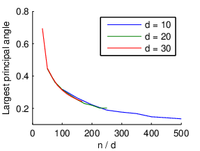
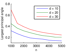
(a) sin⁡(dP)\sin(d_{P}) vs. nn (b) sin⁡(dP)\sin(d_{P}) vs. n/dn/d

Figure 2: Convergence of U^\hat{U} to UU.
Refer to caption
Refer to caption

(a) K=nK=\sqrt{n} (b) K=log⁡(n)K=\log(n)

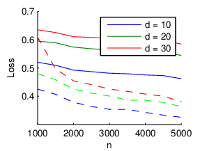
Figure 3: Predicting the expected label given features using KK-NN (RMSE). Dotted lines are for KK-NN after projecting the features XiX_{i} onto U^\hat{U}.

Denote by λ0\lambda_{0} the eigenvalue of multiplicity d−kd-k in Lemma 4. Let Δ=minℓ∈[k]⁡|λ0−λℓ|\Delta=\min_{\ell\in[k]}\left|\lambda_{0}-\lambda_{\ell}\right| be the gap between λ0\lambda_{0} and the remaining eigenvalues. Then, the following lemma holds; this, along with Lemma 4, yields Theorem 1.

Lemma 5.

Let U^\hat{U} be our estimate for UU. If λ1,…,λk\lambda_{1},\dots,\lambda_{k} are separated from λ0\lambda_{0} by at least Δ\Delta, then for ϵ≤min⁡(ϵ0/Δ,14)\epsilon\leq\min(\epsilon_{0}/\Delta,\frac{1}{4}), we have

𝐏𝐫⁡(dP​(U,U^)>ϵ)≤C​exp⁡(−F⁡(Δ​ϵ)),\displaystyle\mathbf{Pr}(d_{P}(U,\hat{U})>\epsilon)\leq C\exp\big(-F(\Delta\epsilon)\big),

where ϵ0\epsilon_{0}, FF are defined as per Lemma 3.

Proof.

If we ensure ‖Q^−Q‖≤Δ/4\|\hat{Q}-Q\|\leq\Delta/4, then, by Weyl’s theorem (Horn and Johnson, 2012), d−kd-k eigenvalues of Q^\hat{Q} are contained in [λk+1−Δ/4,λk+1+Δ/4][\lambda_{k+1}-\Delta/4,\lambda_{k+1}+\Delta/4], and the remaining eigenvalues are outside this set, and will be detected by SpectralMirror. Moreover, by the Davis-Kahan sin⁡(θ)\sin(\theta) theorem,

dp​(range⁡(Q),range⁡(Q^))\displaystyle d_{p}(\mathrm{range}(Q),\mathrm{range}(\hat{Q})) ≤‖Q^−Q‖2Δ−‖Q^−Q‖2=1Δ‖Q^−Q‖2−1.\displaystyle\leq\frac{\|\hat{Q}\!-\!Q\|_{2}}{\Delta-\|\hat{Q}\!-\!Q\|_{2}}=\frac{1}{\frac{\Delta}{\|\hat{Q}\!-\!Q\|_{2}}\!-\!1}.

Thus the event dp​(U,U^)≤ϵd_{p}(U,\hat{U})\leq\epsilon is implied by ‖Q^−Q‖2≤Δ​ϵ1+ϵ≤Δ​ϵ.\|\hat{Q}-Q\|_{2}\leq\frac{\Delta\epsilon}{1+\epsilon}\leq\Delta\epsilon. Moreover, this implies that sufficient condition for ‖Q^−Q‖2≤Δ/4\|\hat{Q}-Q\|_{2}\leq\Delta/4 (which is required for SpectralMirror to detect the correct eigenvalues) is that ϵ≤14\epsilon\leq\frac{1}{4}. The lemma thus follows from Lemma 3. ∎

Note that the Gaussianity of XX is crucially used in the fact that the ‘whitened’ features WW are uncorrelated, which in turn yields Eq. (7). We believe that the theorem can be extended to more general distributions, provided that the transform Σ−12\Sigma^{-\frac{1}{2}} de-correlates the coordinates of XX.

5 Experiments

Refer to caption
Refer to caption
Refer to caption

(a) EM Prediction (close to gr. truth) (b) EM Prediction (random) (c) Clustering (random)

Figure 4: (a) Predicting the label given features and the classifier using using EM (normalized 0-1 loss) from a starting point close to ground truth. Dotted lines are for kNN after projecting the features onto the estimated subspace. (b) Predicting the label given features and the classifier using using EM (normalized 0-1 loss) from a random starting point. (c) Predicting the classifier given features and the label.

We conduct computational experiments to validate the performance of SpecralMirror on subspace estimation, prediction, and clustering. We generate synthetic data using k=2k=2, with profiles uℓ∼𝒩(0,I),ℓ=1,2u_{\ell}\sim\mathcal{N}(0,I),\,\ell=1,2 and mixture weights pℓp_{\ell} sampled uniformly at random from the kk-dimensional simplex. Features are also Gaussian: Xi∼𝒩(0,I),i=1,…,nX_{i}\sim\mathcal{N}(0,I),\,i=1,\dots,n; labels generated by the ℓ\ell-th classifier are given by yi=sgn(uℓTXi),i=1,…,ny_{i}=\sign(u_{\ell}^{T}X_{i}),\,i=1,\dots,n.

Convergence. We study first how well SpectralMirror estimates the span UU. Figure 2(a) shows the convergence of U^\hat{U} to UU in terms of (the sin of) the largest principal angle between the subspaces versus the sample size nn. We also plot the convergence versus the effective sample size n/dn/d (Figure 2(a)). The curves for different values of dd align in Figure 2, indicating that the upper bound in Thm. 1 correctly predicts the sample complexity as n≈Θ⁡(d)n\approx\Theta(d). Though not guaranteed by Theorem 1, in all experiments rr was indeed spanned by U^\hat{U}, so the addition of r^\hat{r} to U^\hat{U} was not necessary.

Prediction through KK-NN. Next, we use the estimated subspace to aid in the prediction of expected labels. Given a new feature vector XX, we use the average label of its KK nearest neighbors (KK-NN) in the training set to predict its expected label. We do this for two settings: once over the raw data (the ‘ambient’ space), and once over data for which the features XX are first projected to U^\hat{U}, the estimated span (of dimension 2). For each nn, we repeat this procedure 25 times with K=nK=\sqrt{n} and K=log⁡nK=\log n. We record the average root mean squared error between predicted and expected labels over the 25 runs. Figures 3(a) and 3(b) show that, despite the error in U^\hat{U}, using KK-NN on this subspace outperforms KK-NN on the ambient space.

Prediction and Clustering through EM. We next study the performance of prediction and clustering using the Expectation-Maximization (EM) algorithm. We use EM to fit the individual profiles both over the training set, as well as on the dataset projected to the estimated subspace U^\hat{U}. We conducted two experiments in this setting: (a) initialize EM close to the true profiles uℓu_{\ell}, ℓ∈[k]\ell\in[k], and (b) randomly initialize EM and choose the best set of profiles from 30 runs. For each nn we run EM 10 times.

The first set of prediction experiments, we again compare expected labels to the predicted labels, using for the latter profiles uℓu_{\ell} and mixture probabilities pℓp_{\ell} as estimated by EM. Figure 4(a) measures the statistical efficiency of EM over the estimated subspace versus EM over the ambient space, when EM is initialized close to the true profiles. The second set of experiments, illustrated in Figure 4(b), aims to capture the additional improvement due to the reduction in the number of local minima in the reduced space. In both cases we see that constraining the estimated profiles to lie in the estimated subspace improves the statistical efficiency of EM; in the more realistic random start experiments, enforcing the subspace constraint also improves the performance of EM by reducing the number of local minima. We also observe an overall improvement compared to prediction through KK-NN.

Finally, we use the fitted profiles uℓu_{\ell} to identify the classifier generating a label given the features and the label. To do this, once the profiles uℓu_{\ell} have been detected by EM, we use a logistic model margin condition to identify the classifier who generated a label, given the label and its features. Figure 4(c) shows the result for EM initialized at a random point, after choosing the best set of profiles from out of 30 runs. We evaluate the performance of this clustering procedure using the normalized 0-1 loss. Again, constraining the estimated profiles to the estimated subspace significantly improves the performance of this clustering task.

6 Conclusions

We have proposed SpectralMirror, a method for discovering the span of a mixture of linear classifiers. Our method relies on a non-linear transform of the labels, which we refer to as ‘mirroring’. Moreover, we have provided consistency guarantees and non-asymptotic bounds, that also imply the near optimal statistical efficiency of the method. Finally, we have shown that, despite the fact that SpectralMirror discovers the span only approximately, this is sufficient to allow for a significant improvement in both prediction and clustering, when the features are projected to the estimated span.

We have already discussed several technical issues that remain open, and that we believe are amenable to further analysis. These include amending the Gaussianity assumption, and applying our bounds to other pHd-inspired methods. An additional research topic is to further improve the computational complexity of the estimation of the eigenvectors of the ‘mirrored’ matrix Q^\hat{Q}. This is of greatest interest in cases where the covariance Σ\Sigma and mean μ\mu are a priori known. This would be the case when, e.g., the method is applied repeatedly and, although the features XX are sampled from the same distribution each time, labels YY are generated from a different mixture of classifiers. In this case, SpectralMirror lacks the pre-processing step, that requires estimating Σ\Sigma and is thus computationally intensive; the remaining operations amount to discovering the spectrum of Q^\hat{Q}, an operation that can be performed more efficiently. For example, we can use a regularized M-estimator to exploit the fact that Σ−1/2Q^Σ−1/2\Sigma^{-1/2}\hat{Q}\Sigma^{-1/2} should be the sum of a multiple of the identity and a low rank matrix—see, e.g., Negahban et al. (2012).

References

  • Anandkumar et al. (2012) [author] Anandkumar, AnimaA., Ge, RongR., Hsu, DanielD., Kakade, Sham MS. M. and Telgarsky, MatusM. (2012). Tensor decompositions for learning latent variable models. arXiv preprint arXiv:1210.7559. \endbibitem
  • Arora and Kannan (2001) {binproceedings}[author] Arora, SanjeevS. and Kannan, RaviR. (2001). Learning mixtures of arbitrary gaussians. In Proceedings of the thirty-third annual ACM symposium on Theory of computing 247–257. ACM. \endbibitem
  • Bartholomew, Knott and Moustaki (2011) [author] Bartholomew, David JD. J., Knott, MartinM. and Moustaki, IriniI. (2011). Latent variable models and factor analysis: A unified approach 899. Wiley. com. \endbibitem
  • Bishop (1998) [author] Bishop, Christopher MC. M. (1998). Latent variable models. In Learning in graphical models 371–403. Springer. \endbibitem
  • Chaganty and Liang (2013) {binproceedings}[author] Chaganty, Arun TejasviA. T. and Liang, PercyP. (2013). Spectral experts for estimating mixtures of linear regressions. In ICML. \endbibitem
  • Cook (1998) [author] Cook, R DennisR. D. (1998). Principal Hessian directions revisited. Journal of the American Statistical Association 93 84–94. \endbibitem
  • Dempster, Laird and Rubin (1977) [author] Dempster, Arthur PA. P., Laird, Nan MN. M. and Rubin, Donald BD. B. (1977). Maximum likelihood from incomplete data via the EM algorithm. Journal of the Royal Statistical Society. Series B (Methodological) 1–38. \endbibitem
  • Horn and Johnson (2012) [author] Horn, Roger AR. A. and Johnson, Charles RC. R. (2012). Matrix analysis. Cambridge university press. \endbibitem
  • Hsu, Kakade and Zhang (2012) [author] Hsu, DanielD., Kakade, Sham MS. M. and Zhang, TongT. (2012). A spectral algorithm for learning hidden Markov models. Journal of Computer and System Sciences 78 1460–1480. \endbibitem
  • Jordan and Jacobs (1994) [author] Jordan, Michael IM. I. and Jacobs, Robert AR. A. (1994). Hierarchical mixtures of experts and the EM algorithm. Neural computation 6 181–214. \endbibitem
  • Li (1992) [author] Li, Ker-ChauK.-C. (1992). On principal Hessian directions for data visualization and dimension reduction: another application of Stein’s lemma. Journal of the American Statistical Association 87 1025–1039. \endbibitem
  • Liang et al. (2006) {binproceedings}[author] Liang, PercyP., Bouchard-Côté, AlexandreA., Klein, DanD. and Taskar, BenB. (2006). An end-to-end discriminative approach to machine translation. In Proceedings of the 21st International Conference on Computational Linguistics and the 44th annual meeting of the Association for Computational Linguistics 761–768. Association for Computational Linguistics. \endbibitem
  • Liu (1994) [author] Liu, Jun SJ. S. (1994). Siegel’s formula via Stein’s identities. Statistics &amp; Probability Letters 21 247–251. \endbibitem
  • McLachlan and Peel (2004) [author] McLachlan, GeoffreyG. and Peel, DavidD. (2004). Finite mixture models. Wiley. com. \endbibitem
  • Moitra and Valiant (2010) {binproceedings}[author] Moitra, AnkurA. and Valiant, GregoryG. (2010). Settling the polynomial learnability of mixtures of gaussians. In Foundations of Computer Science (FOCS), 2010 51st Annual IEEE Symposium on 93–102. IEEE. \endbibitem
  • Negahban et al. (2012) [author] Negahban, Sahand NS. N., Ravikumar, PradeepP., Wainwright, Martin JM. J. and Yu, BinB. (2012). A unified framework for high-dimensional analysis of MM-estimators with decomposable regularizers. Statistical Science 27 538–557. \endbibitem
  • Pearson (1894) [author] Pearson, KarlK. (1894). Contributions to the mathematical theory of evolution. Philosophical Transactions of the Royal Society of London. A 185 71–110. \endbibitem
  • Quattoni, Collins and Darrell (2004) {binproceedings}[author] Quattoni, AriadnaA., Collins, MichaelM. and Darrell, TrevorT. (2004). Conditional random fields for object recognition. In Advances in neural information processing systems 1097–1104. \endbibitem
  • Stein (1973) {binproceedings}[author] Stein, Charles MC. M. (1973). Estimation of the mean of a multivariate normal distribution. In Prague Symposium on Asymptotic Statistics. \endbibitem
  • Vershynin (2010) [author] Vershynin, R.R. (2010). Introduction to the non-asymptotic analysis of random matrices. arXiv preprint arXiv:1011.3027. \endbibitem
  • Zelnik-Manor and Perona (2004) {binproceedings}[author] Zelnik-Manor, LihiL. and Perona, PietroP. (2004). Self-tuning spectral clustering. In Advances in neural information processing systems 1601–1608. \endbibitem

Appendix A A Large-Deviation Lemma

We first prove a Bernstein-type inequality for sub-Gaussian random vectors, that we shall use in our proofs:

Lemma 6.

Let X∈ℝdX\in\mathbb{R}^{d} be a sub-Gaussian random vector, i.e. ⟨a,X⟩\langle a,X\rangle is sub-Gaussian for any a∈ℝda\in\mathbb{R}^{d}. Then there exist universal constants c1,c2c_{1},c_{2} such that

𝐏𝐫⁡(‖X‖2≥t)\displaystyle\mathbf{Pr}(\left\|X\right\|_{2}\geq t) ≤\displaystyle\leq
c1exp(−min\displaystyle c_{1}\exp\bigg(-\min OPEN{c2​(t2−d​‖Σ‖2)4​d​‖X‖ψ22,(t2−d​‖Σ‖2)264​c2​‖X‖ψ24}).\displaystyle\left\{\frac{c_{2}(t^{2}-d\left\|\Sigma\right\|_{2})}{4d\left\|X\right\|_{\psi_{2}}^{2}},\frac{(t^{2}-d\left\|\Sigma\right\|_{2})^{2}}{64c_{2}\left\|X\right\|_{\psi_{2}}^{4}}\right\}\bigg).
Proof.

By the (exponential) Markov inequality, we have

𝐏𝐫⁡(‖X‖2≥t)=𝐏𝐫⁡(exp⁡(λ​‖X‖22)≥exp⁡(λ​t2))≤𝐄⁡[exp⁡(λ​‖X‖22)]exp⁡(λ​t2).\begin{split}\mathbf{Pr}(\left\|X\right\|_{2}\geq t)=\mathbf{Pr}(\exp(\lambda\left\|X\right\|_{2}^{2})\geq\exp(\lambda t^{2}))\\ \leq\frac{\Expect[\exp(\lambda\left\|X\right\|_{2}^{2})]}{\exp(\lambda t^{2})}.\end{split} (10)

Let ZZ be uniformly distributed on the unit sphere 𝐒d−1\mathbf{S}^{d-1}. Then d​Z\sqrt{d}Z is isotropic so d​𝐄⁡[⟨Z,a⟩2]=‖a‖22d\Expect[\langle Z,a\rangle^{2}]=\left\|a\right\|_{2}^{2} for all aa. We use this fact to bound the m.g.f. of ‖X‖22\left\|X\right\|_{2}^{2}:

𝐄⁡[exp⁡(λ​‖X‖22)]\displaystyle\Expect[\exp(\lambda\left\|X\right\|_{2}^{2})] =𝐄X⁡[exp⁡(λ​d​𝐄Z​[⟨Z,X⟩2])]\displaystyle=\Expect_{X}[\exp(\lambda d\Expect_{Z}[\langle Z,X\rangle^{2}])]
≤𝐄X⁡[𝐄Z⁡[exp⁡(λ​d​⟨Z,X⟩2)]].\displaystyle\leq\Expect_{X}[\Expect_{Z}[\exp(\lambda d\langle Z,X\rangle^{2})]].

We interchange the order of expectation to obtain

𝐄⁡[exp⁡(λ​‖X‖22)]\displaystyle\Expect[\exp(\lambda\left\|X\right\|_{2}^{2})] ≤𝐄Z⁡[𝐄X⁡[exp⁡(λ​d​⟨X,Z⟩2)]]\displaystyle\leq\Expect_{Z}[\Expect_{X}[\exp(\lambda d\langle X,Z\rangle^{2})]]
≤sup{𝐄X⁡[exp⁡(λ​d​⟨X,Z⟩2)]∣z∈𝐒d−1}.\displaystyle\leq\sup\,\{\Expect_{X}[\exp(\lambda d\langle X,Z\rangle^{2})]\mid z\in\mathbf{S}^{d-1}\}.

⟨X,z⟩\langle X,z\rangle is sub-Gaussian (for fixed zz) so ⟨X,z⟩2\langle X,z\rangle^{2} is (noncentered) sub-exponential. If λ​d<c/‖⟨X,z⟩2−𝐄⁡[⟨X,z⟩2]‖ψ1\lambda d<c/\left\|\langle X,z\rangle^{2}-\Expect[\langle X,z\rangle^{2}]\right\|_{\psi_{1}}, then

𝐄⁡[exp⁡(λ​d​⟨X,z⟩2)]\displaystyle\Expect[\exp(\lambda d\langle X,z\rangle^{2})]
≤exp⁡(λ​d​𝐄⁡[⟨X,z⟩2])​𝐄​[exp⁡(λ​d​(⟨X,z⟩2−𝐄⁡[⟨X,z⟩2]))]\displaystyle\leq\exp(\lambda d\Expect[\langle X,z\rangle^{2}])\Expect[\exp(\lambda d(\langle X,z\rangle^{2}-\Expect[\langle X,z\rangle^{2}]))]
≤exp⁡(λ​d​𝐄⁡[⟨X,z⟩2]+cd2​λ2​‖⟨X,z⟩2−𝐄⁡[⟨X,z⟩2]‖ψ12)\displaystyle\leq\exp(\lambda d\Expect[\langle X,z\rangle^{2}]+cd^{2}\lambda^{2}\left\|\langle X,z\rangle^{2}-\Expect[\langle X,z\rangle^{2}]\right\|_{\psi_{1}}^{2})
≤exp⁡(λ​d​𝐄⁡[⟨X,z⟩2]+4​c​d2​λ2​‖⟨X,z⟩2‖ψ12)\displaystyle\leq\exp(\lambda d\Expect[\langle X,z\rangle^{2}]+4cd^{2}\lambda^{2}\left\|\langle X,z\rangle^{2}\right\|_{\psi_{1}}^{2})
≤exp⁡(λ​d​𝐄⁡[⟨X,z⟩2]+16​c​d2​λ2​‖⟨X,z⟩‖ψ24).\displaystyle\leq\exp(\lambda d\Expect[\langle X,z\rangle^{2}]+16cd^{2}\lambda^{2}\left\|\langle X,z\rangle\right\|_{\psi_{2}}^{4}). (11)

We substitute this bound into (10) to obtain

𝐏𝐫⁡(‖X‖2≥t)≤exp⁡(16​c​d2​λ2​‖X‖ψ24+λ⁡(d​‖Σ‖2−t2)),\mathbf{Pr}(\left\|X\right\|_{2}\geq t)\leq\\ \exp(16cd^{2}\lambda^{2}\left\|X\right\|^{4}_{\psi_{2}}+\lambda(d\left\|\Sigma\right\|_{2}-t^{2})),

where Σ\Sigma is the covariance matrix of XX. We optimize over λ\lambda to obtain

𝐏𝐫⁡(‖X‖2≥t)≤e−(t2−d​‖Σ‖2)264​c​d2​‖X‖ψ24.\mathbf{Pr}(\left\|X\right\|_{2}\geq t)\leq e^{-\frac{(t^{2}-d\left\|\Sigma\right\|_{2})^{2}}{64cd^{2}\left\|X\right\|_{\psi_{2}}^{4}}}.

If the optimum lies outside the region where the m.g.f. bound holds (11), we can always choose

λ=c4​d​‖X‖ψ22≤cd​‖⟨X,z⟩2−𝐄⁡[⟨X,z⟩2]‖ψ1\lambda=\frac{c}{4d\left\|X\right\|_{\psi_{2}}^{2}}\leq\frac{c}{d\left\|\langle X,z\rangle^{2}-\Expect[\langle X,z\rangle^{2}]\right\|_{\psi_{1}}}

in to obtain the tail bound:

𝐏𝐫⁡(‖X‖2≥t)≤ec3+c⁡(d​‖Σ‖2−t2)4​d​‖X‖ψ22.\mathbf{Pr}(\left\|X\right\|_{2}\geq t)\leq e^{c^{3}+\frac{c(d\left\|\Sigma\right\|_{2}-t^{2})}{4d\left\|X\right\|_{\psi_{2}}^{2}}}.

We combine these two bounds to obtain

𝐏𝐫⁡(‖X‖2≥t)≤c1​e−min⁡{c2​(t2−d​‖Σ‖2)4​d​‖X‖ψ22,(t2−d​‖Σ‖2)264​c2​‖X‖ψ24}.\mathbf{Pr}(\left\|X\right\|_{2}\geq t)\leq c_{1}e^{-\min\left\{\frac{c_{2}(t^{2}-d\left\|\Sigma\right\|_{2})}{4d\left\|X\right\|_{\psi_{2}}^{2}},\frac{(t^{2}-d\left\|\Sigma\right\|_{2})^{2}}{64c_{2}\left\|X\right\|_{\psi_{2}}^{4}}\right\}}.

Note that the t2t^{2} bound always holds. However, for small tt, the t4t^{4} term yields a tighter bound. ∎

Appendix B Proof of Lemma 1 (Weak Conv. of r^\hat{r})

Proof.

We expand r^n−r\hat{r}_{n}-r (and neglect higher order terms) to obtain

‖r^n−r‖2\displaystyle\left\|\hat{r}_{n}-r\right\|_{2} =‖1n​∑i=1nΣ^−1​Yi​(Xi−μ^)−Σ−1​𝐄⁡[s⁡(X)​(X−μ)]‖2\displaystyle=\Bigl\|\frac{1}{n}\sum_{i=1}^{n}\hat{\Sigma}^{-1}Y_{i}(X_{i}-\hat{\mu})-\Sigma^{-1}\Expect[s(X)(X-\mu)]\Bigr\|_{2}
≤‖Σ^−1‖2​‖1n​∑i=1nYi​(Xi−μ^)−𝐄⁡[s⁡(X)​(X−μ)]‖2\displaystyle\leq\left\|\hat{\Sigma}^{-1}\right\|_{2}\Bigl\|\frac{1}{n}\sum_{i=1}^{n}Y_{i}(X_{i}-\hat{\mu})-\Expect[s(X)(X-\mu)]\Bigr\|_{2}
+‖𝐄⁡[s⁡(X)​(X−μ)]‖2​‖Σ^−1−Σ−1‖2+(oP​(1))2.\displaystyle\hskip 12.0pt+\|\Expect[s(X)(X-\mu)]\|_{2}\|\hat{\Sigma}^{-1}-\Sigma^{-1}\|_{2}+(o_{P}(1))^{2}. (12)

The higher order terms generically look like

𝐏𝐫⁡(|X−𝐄⁡[X]|​|Y−𝐄⁡[Y]|>ϵ).\mathbf{Pr}(\left|X-\Expect[X]\right|\left|Y-\Expect[Y]\right|>\epsilon). (13)

We apply the union bound to deduce

𝐏𝐫⁡(|X−𝐄⁡[X]|​|Y−𝐄⁡[Y]|>ϵ)\displaystyle\mathbf{Pr}(\left|X-\Expect[X]\right|\left|Y-\Expect[Y]\right|>\epsilon)
≤𝐏𝐫⁡(|X−𝐄⁡[X]|>ϵ)+𝐏𝐫⁡(|X−𝐄⁡[X]|>ϵ).\displaystyle\hskip 12.0pt\leq\mathbf{Pr}(\left|X-\Expect[X]\right|>\sqrt{\epsilon})+\mathbf{Pr}(\left|X-\Expect[X]\right|>\sqrt{\epsilon}).

For any ϵ<1\epsilon<1, ϵ>ϵ\sqrt{\epsilon}>\epsilon and we have

𝐏𝐫⁡(|X−𝐄⁡[X]|>ϵ)≤𝐏𝐫⁡(|X−𝐄⁡[X]|>ϵ).\mathbf{Pr}(\left|X-\Expect[X]\right|>\sqrt{\epsilon})\leq\mathbf{Pr}(\left|X-\Expect[X]\right|>\epsilon).

Since terms of the form 𝐏𝐫⁡(|X−𝐄⁡[X]|>ϵ)\mathbf{Pr}(\left|X-\Expect[X]\right|>\epsilon) appear in the upper bounds we derive, we can handle terms like (13) with a constant factor (say 2). Since our bounds involve multiplicative constant factors anyways, we neglect these terms to simplify our derivation.

We expand the first term to obtain

‖1n​∑i=1nYi​(Xi−μ^)−𝐄⁡[Y⁡(X−μ)]‖2\displaystyle\Bigl\|\frac{1}{n}\sum_{i=1}^{n}Y_{i}(X_{i}-\hat{\mu})-\Expect[Y(X-\mu)]\Bigr\|_{2}
≤|𝐄⁡[s⁡(X)]|​‖μ^−μ‖2+‖μ‖2|1n​∑i=1nYi−𝐄⁡[s⁡(X)]|2\displaystyle\hskip 12.0pt\leq|\Expect[s(X)]|\left\|\hat{\mu}-\mu\right\|_{2}+\left\|\mu\right\|_{2}\Bigl|\frac{1}{n}\sum_{i=1}^{n}Y_{i}-\Expect[s(X)]\Bigr|_{2}
+‖1n​∑i=1nYi​(Xi−μ)−𝐄⁡[s⁡(X)​(X−μ)]‖2\displaystyle\hskip 12.0pt\hskip 12.0pt+\Bigl\|\frac{1}{n}\sum_{i=1}^{n}Y_{i}(X_{i}-\mu)-\Expect[s(X)(X-\mu)]\Bigr\|_{2}
+(oP​(1))2.\displaystyle\hskip 12.0pt\hskip 12.0pt+(o_{P}(1))^{2}.

μ^−μ\hat{\mu}-\mu is a sub-Gaussian random variable with sub-Gaussian norm ‖X‖ψ2n\frac{\left\|X\right\|_{\psi_{2}}}{\sqrt{n}}, so there exist universal c1c_{1} and c2c_{2} s.t.

𝐏𝐫⁡(‖μ^−μ‖2>t)≤c1​exp⁡(−c2​n​(t2−d​‖Σ‖2)4​d​‖X‖ψ22).\mathbf{Pr}(\left\|\hat{\mu}-\mu\right\|_{2}>t)\leq c_{1}\exp\left(-\frac{c_{2}n(t^{2}-d\left\|\Sigma\right\|_{2})}{4d\left\|X\right\|_{\psi_{2}}^{2}}\right).

YY is bounded between 1 and -1, so

  1. 1.

    We can use Chernoff’s inequality to deduce

    𝐏𝐫(|1n∑i=1nYi−𝐄[s(X)]|>t)≤2exp(−nt2/2).\mathbf{Pr}\biggl(\Bigl|\frac{1}{n}\sum_{i=1}^{n}Y_{i}-\Expect[s(X)]\Bigr|>t\bigr)\leq 2\exp(-nt^{2}/2).
  2. 2.

    Yi​(Xi−μ)Y_{i}(X_{i}-\mu) are sub-Gaussian. Thus there exist universal c1c_{1} and c2c_{2} such that

    𝐏𝐫⁡(‖1n​∑i=1nYi​(Xi−μ)−𝐄⁡[s⁡(X)​(X−μ)]‖2>t)≤c1​exp⁡(−c2​n​(t2−d​‖Σ‖2)4​d​‖X‖ψ22).\displaystyle\begin{split}\mathbf{Pr}\biggl(\Bigl\|\frac{1}{n}\sum_{i=1}^{n}Y_{i}(X_{i}-\mu)-\Expect[s(X)(X-\mu)]\Bigr\|_{2}>t\bigr)\leq\\ c_{1}\exp\left(-\frac{c_{2}n(t^{2}-d\left\|\Sigma\right\|_{2})}{4d\left\|X\right\|_{\psi_{2}}^{2}}\right).\end{split}

We expand the second term in (12) to obtain

∥Σ^−1−Σ−1∥=∥Σ−1/2∥∥Σ1/2Σ^−1Σ1/2−I∥∥Σ−1/2∥.\displaystyle\|\hat{\Sigma}^{-1}-\Sigma^{-1}\|=\|\Sigma^{-1/2}\|\|\Sigma^{1/2}\hat{\Sigma}^{-1}\Sigma^{1/2}-I\|\|\Sigma^{-1/2}\|.

We expand the middle term to obtain

∥Σ−1/2Σ^Σ−1/2−I∥\displaystyle\|\Sigma^{-1/2}\hat{\Sigma}\Sigma^{-1/2}-I\|
≤∥(1n∑i=1nΣ−1/2(Xi−μ)(Xi−μ)TΣ−1/2)−1−I∥2\displaystyle\hskip 12.0pt\leq\Bigl\|\Bigl(\frac{1}{n}\sum_{i=1}^{n}\Sigma^{-1/2}(X_{i}-\mu)(X_{i}-\mu)^{T}\Sigma^{-1/2}\Bigr)^{-1}-I\Bigr\|_{2}
+2​‖μ‖2​‖μ^−μ‖2+(oP​(1))2\displaystyle\hskip 12.0pt\hskip 12.0pt+2\left\|\mu\right\|_{2}\left\|\hat{\mu}-\mu\right\|_{2}+(o_{P}(1))^{2}

We use Theorem 5.39 in Vershynin (2010) to bound the first term:

𝐏𝐫⁡(‖1n​∑i=1nWi​WiT−I‖2>t)≤2​exp⁡(−c1′​(n​t−c2′​d)2),\mathbf{Pr}\biggl(\Bigl\|\frac{1}{n}\sum_{i=1}^{n}W_{i}W_{i}^{T}-I\Bigr\|_{2}>t\Bigr)\leq 2\exp(-c_{1}^{\prime}(\sqrt{n}t-c_{2}^{\prime}\sqrt{d})^{2}),

where c1′,c2′c_{1}^{\prime},c_{2}^{\prime} depend on the sub-Gaussian norm of WW. We substitute these bounds into our expression for ‖r^−r‖2\|\hat{r}-r\|_{2} to deduce

𝐏𝐫⁡(‖r^−r‖2≥ϵ)≤C​e−min⁡{c1​n​ϵ2d,(c1′​n​ϵ−c2′​d)2},\textstyle\mathbf{Pr}(\|\hat{r}\!-\!r\|_{2}\geq\epsilon)\leq Ce^{-\min\left\{\frac{c_{1}n\epsilon^{2}}{d},\bigl(c_{1}^{\prime}\sqrt{n}\epsilon-c_{2}^{\prime}\sqrt{d}\bigr)^{2}\right\}},

where CC is an absolute constant and c1,c1′,c2′c_{1},c_{1}^{\prime},c_{2}^{\prime} depend on the sub-Gaussian norm of XX. ∎

Appendix C Proof of Lemma 3 (Weak Conv. of Q^\hat{Q})

Let r~\tilde{r} denote the projection of rr onto UU.

Lemma 7.

If

‖r^−r‖2≤ϵ0=min⁡{α1,…,αk}​σmin​(U),\|\hat{r}-r\|_{2}\leq\epsilon_{0}=\min\,\{\alpha_{1},\ldots,\alpha_{k}\}\sigma_{\min}(U),

then r~\tilde{r} lies in the interior of the positive cone spanned by (uℓ)ℓ∈[k](u_{\ell})_{\ell\in[k]}, where σmin​(U)\sigma_{\min}(U) is the smallest nonzero singular value of UU.

Proof.

rr lies in interior of the conic hull of {u1,…,uk}\{u_{1},\dots,u_{k}\}, so we can express rr as ∑i=1kαi​ui\sum_{i=1}^{k}\alpha_{i}u_{i}, where ri>0r_{i}>0. If r~\tilde{r} also lies in the conic hull, then r~=∑i=1kβi​ui\tilde{r}=\sum_{i=1}^{k}\beta_{i}u_{i} for some βi>0\beta_{i}>0. Then

‖r~−r‖2=‖∑i=1k(αi−βi)​ui‖2=(α−β)T​U​UT​(α−β)\displaystyle\left\|\tilde{r}-r\right\|_{2}=\|\sum_{i=1}^{k}(\alpha_{i}-\beta_{i})u_{i}\|_{2}=\sqrt{(\alpha-\beta)^{T}UU^{T}(\alpha-\beta)}
≥‖α−β‖2​σmin​(U)≥‖α−β‖∞​σmin​(U).\displaystyle\geq\left\|\alpha-\beta\right\|_{2}\sigma_{\min}(U)\geq\left\|\alpha-\beta\right\|_{\infty}\sigma_{\min}(U).

To ensure β\beta is component-wise positive, we must have ‖α−β‖∞<min⁡{α1,…,αk}\left\|\alpha-\beta\right\|_{\infty}<\min\{\alpha_{1},\dots,\alpha_{k}\}. A sufficient condition is ‖r~−r‖2≤ϵ0≤min⁡{α1,…,αk}​σmin​(U)\left\|\tilde{r}-r\right\|_{2}\leq\epsilon_{0}\leq\min\{\alpha_{1},\dots,\alpha_{k}\}\sigma_{\min}(U). ∎

We are now ready to prove Lemma 3. We expand ‖Q^n−Q‖2\|\hat{Q}_{n}-Q\|_{2} (and neglect higher order terms) to obtain

∥Q^n\displaystyle\|\hat{Q}_{n} −Q∥2≤\displaystyle-Q\|_{2}\leq
∥1n∑i=1nZiΣ−1/2(Xi−μ)(Xi−μ)TΣ−1/2−Q∥2\displaystyle\Bigl\|\frac{1}{n}\sum_{i=1}^{n}Z_{i}\Sigma^{-1/2}(X_{i}-\mu)(X_{i}-\mu)^{T}\Sigma^{-1/2}-Q\Bigr\|_{2}
+2∥Σ^−1/2−Σ−1/2∥2𝐄[∥(X−μ)(X−μ)Σ−1/2∥2]\displaystyle\hskip 12.0pt+2\|\hat{\Sigma}^{-1/2}-\Sigma^{-1/2}\|_{2}\Expect\bigl[\|(X-\mu)(X-\mu)\Sigma^{-1/2}\|_{2}\bigr]
+2∥Σ−1/2∥2∥μ^−μ∥2𝐄[∥(X−μ)Σ−1/2∥2]\displaystyle\hskip 12.0pt+2\|\Sigma^{-1/2}\|_{2}\|\hat{\mu}-\mu\|_{2}\Expect\bigl[\|(X-\mu)\Sigma^{-1/2}\|_{2}\bigr]
+(oP​(1))2.\displaystyle\hskip 12.0pt+(o_{P}(1))^{2}.

The second and third terms can be bounded using the same bounds used in the analysis of how fast r^\hat{r} converges to rr. Thus we focus on how fast

∑i=1nZiΣ−1/2(Xi−μ)(Xi−μ)TΣ−1/2\sum_{i=1}^{n}Z_{i}\Sigma^{-1/2}(X_{i}-\mu)(X_{i}-\mu)^{T}\Sigma^{-1/2}

coverges to QQ. Let ϵ′=min⁡(ϵ0,r2)\epsilon^{\prime}=\min(\epsilon_{0},\frac{r}{2}). First, we note that

𝐏𝐫⁡(‖1n​∑i=1nZi​Wi​WiT−Q‖2>t)\displaystyle\mathbf{Pr}\biggl(\Bigl\|\frac{1}{n}\sum_{i=1}^{n}Z_{i}W_{i}W_{i}^{T}-Q\Bigr\|_{2}>t\Bigr) (14)
≤𝐏𝐫⁡(‖1n​∑i=1nZi​Wi​WiT−Q‖2>t∣r^∈Bϵ′​(r))​𝐏𝐫​(r^∈Bϵ′​(r))\displaystyle\hskip 12.0pt\leq\mathbf{Pr}\biggl(\Bigl\|\frac{1}{n}\sum_{i=1}^{n}Z_{i}W_{i}W_{i}^{T}-Q\Bigr\|_{2}>t\mid\hat{r}\in B_{\epsilon^{\prime}}(r)\Bigr)\mathbf{Pr}(\hat{r}\in B_{\epsilon^{\prime}}(r))
+𝐏𝐫⁡(r^∉Bϵ′​(r)).\displaystyle\hskip 12.0pt\hskip 12.0pt+\mathbf{Pr}(\hat{r}\notin B_{\epsilon^{\prime}}(r)).

Let Z~i\tilde{Z}_{i} denote the “corrected” version of the ZiZ_{i}’s, i.e. the ZiZ_{i}’s we obtain if we use the projection of r^\hat{r} onto UU to flip the labels, and WiW_{i} denote Σ−1/2(Xi−μ)\Sigma^{-1/2}(X_{i}-\mu). We have

‖1n​∑i=1nZi​Wi​WiT−Q‖2\displaystyle\Bigl\|\frac{1}{n}\sum_{i=1}^{n}Z_{i}W_{i}W_{i}^{T}-Q\Bigr\|_{2} (15)
≤‖1n​∑i=1nZ~i​Wi​WiT−Q‖2+‖1n​∑i=1n(Zi−Z~i)​Wi​WiT‖2.\displaystyle\hskip 12.0pt\leq\Bigl\|\frac{1}{n}\sum_{i=1}^{n}\tilde{Z}_{i}W_{i}W_{i}^{T}-Q\Bigr\|_{2}+\Bigl\|\frac{1}{n}\sum_{i=1}^{n}(Z_{i}-\tilde{Z}_{i})W_{i}W_{i}^{T}\Bigr\|_{2}.

The probability the first term is large is bounded by

𝐏𝐫⁡(‖1n​∑i=1nZ~i​Wi​WiT−Q‖2>t∣r^∈Bϵ′​(r))\displaystyle\mathbf{Pr}\biggl(\Bigl\|\frac{1}{n}\sum_{i=1}^{n}\tilde{Z}_{i}W_{i}W_{i}^{T}-Q\Bigr\|_{2}>t\mid\hat{r}\in B_{\epsilon^{\prime}}(r)\Bigr) (16)
≤supr^∈Bϵ0​(r)𝐏𝐫⁡(‖1n​∑i=1nZ~i​Wi​WiT−Q‖2>t∣r^∈Bϵ′​(r))\displaystyle\hskip 12.0pt\leq\sup_{\hat{r}\in B_{\epsilon_{0}}(r)}\mathbf{Pr}\biggl(\Bigl\|\frac{1}{n}\sum_{i=1}^{n}\tilde{Z}_{i}W_{i}W_{i}^{T}-Q\Bigr\|_{2}>t\mid\hat{r}\in B_{\epsilon^{\prime}}(r)\Bigr)

The ZiZ_{i}’s are independent of WiW_{i}’s because the ZiZ_{i}’s were computed using r^\hat{r} that was in turn computed independently of the XiX_{i}’s, as the former are computed on a different partition of [n][n]. Thus, the sum in the r.h.s. of (15) is a sum of i.i.d. r.v. and can be bounded by

supr^∈Bϵr​(r)𝐏𝐫⁡(‖1n​∑i=1nZ~i​Wi​WiT−Q‖2>t∣r^∈Bϵ′​(r))\displaystyle\sup_{\hat{r}\in B_{\epsilon_{r}}(r)}\mathbf{Pr}\biggl(\Bigl\|\frac{1}{n}\sum_{i=1}^{n}\tilde{Z}_{i}W_{i}W_{i}^{T}-Q\Bigr\|_{2}>t\mid\hat{r}\in B_{\epsilon^{\prime}}(r)\bigr)
≤2​exp⁡(−c1​(n​t−c2​d)2),\displaystyle\hskip 12.0pt\leq 2\exp(-c_{1}(\sqrt{n}t-c_{2}\sqrt{d})^{2}),

where c1,c2c_{1},c_{2} depend on the sub-Gaussian norm of Z~​W\tilde{Z}W. This is a consequence of Remark 5.40 in Vershynin (2010).

We now focus on bounding the second term in (15). In what follows, without loss of generality, we will restrict WW to the k+1 subspace spanned by UU and r^\hat{r}, as remaining components of the WiW_{i}’s do not contribute to the computation. Let Cr^C_{\hat{r}} (for cone) be the “bad” region, i.e. the region where Z≠Z~Z\neq\tilde{Z}. We have

‖1n​∑i=1n(Zi−Z~i)​Wi​WiT‖2=‖2n​∑i=1n𝟏Cr^​(Wi)​Wi​WiT‖2.\Bigl\|\frac{1}{n}\sum_{i=1}^{n}(Z_{i}-\tilde{Z}_{i})W_{i}W_{i}^{T}\Bigr\|_{2}=\Bigl\|\frac{2}{n}\sum_{i=1}^{n}\mathbf{1}_{C_{\hat{r}}}(W_{i})W_{i}W_{i}^{T}\Bigr\|_{2}.

By the triangle inequality, we have

‖2n​∑i=1n𝟏Cr^​(Wi)​Wi​WiT‖2\displaystyle\Bigl\|\frac{2}{n}\sum_{i=1}^{n}\mathbf{1}_{C_{\hat{r}}}(W_{i})W_{i}W_{i}^{T}\Bigr\|_{2}
≤2‖𝐄[𝟏Cr^(W)WWT]‖2+∥2n∑i=1n\displaystyle\hskip 12.0pt\leq 2\left\|\Expect[\mathbf{1}_{C_{\hat{r}}}(W)WW^{T}]\right\|_{2}+\Bigl\|\frac{2}{n}\sum_{i=1}^{n} 𝟏Cr^​(Wi)​Wi​WiT\displaystyle\mathbf{1}_{C_{\hat{r}}}(W_{i})W_{i}W_{i}^{T}
−2𝐄[𝟏Cr^(W)WWT]∥2\displaystyle\hskip 12.0pt\hskip 12.0pt-2\Expect[\mathbf{1}_{C_{\hat{r}}}(W)WW^{T}]\Bigr\|_{2} (17)

𝟏Cr^\mathbf{1}_{C_{\hat{r}}} is bounded, hence 𝟏Cr^​(Wi)​Wi\mathbf{1}_{C_{\hat{r}}}(W_{i})W_{i} is sub-Gaussian and

𝐏𝐫(∥2n∑i=1n\displaystyle\mathbf{Pr}\bigg(\Bigl\|\frac{2}{n}\sum_{i=1}^{n} 𝟏Cr^​(Wi)​Wi​WiT\displaystyle\mathbf{1}_{C_{\hat{r}}}(W_{i})W_{i}W_{i}^{T}
−2𝐄[𝟏Cr^(W)WWT]∥2>t∣r^∈Bϵ′(r))\displaystyle-2\Expect[\mathbf{1}_{C_{\hat{r}}}(W)WW^{T}]\Bigr\|_{2}>t\mid\hat{r}\in B_{\epsilon^{\prime}}(r)\bigg)
≤2​exp⁡(−c1​(n​t−c2​d)2),\displaystyle\hskip 12.0pt\leq 2\exp(-c_{1}(\sqrt{n}t-c_{2}\sqrt{d})^{2}), (18)

where c1,c2c_{1},c_{2} depend on the sub-Gaussian norm of XX. It remains to bound ‖𝐄⁡[𝟏Cr^​(W)​WWT]‖2\left\|\Expect[\mathbf{1}_{C_{\hat{r}}}(W)WW^{T}]\right\|_{2}.

We use Jensen’s inequality to obtain

‖𝐄⁡[𝟏Cr^​(W)​WWT]‖2≤𝐄⁡[𝟏Cr^​(W)​‖WWT‖2]\displaystyle\hskip 12.0pt\left\|\Expect[\mathbf{1}_{C_{\hat{r}}}(W)WW^{T}]\right\|_{2}\leq\Expect[\mathbf{1}_{C_{\hat{r}}}(W)\left\|WW^{T}\right\|_{2}]
≤C​𝐏𝐫​(W∈Cr^),\displaystyle\hskip 12.0pt\leq C\mathbf{Pr}(W\in C_{\hat{r}}), (19)

where the constant CC depends on kk, as WW is restricted to the space spanned by UU and r^\hat{r}. Finally, we bound 𝐏𝐫⁡(W∈Cr^)\mathbf{Pr}(W\in C_{\hat{r}}).

The distribution of WiW_{i} is spherically symmetric so the probability that Wi∈Cr^W_{i}\in C_{\hat{r}} is proportional to the surface area of the set Cr^∩𝐒kC_{\hat{r}}\cap\mathbf{S}^{k}, where 𝐒k\mathbf{S}^{k} the unit sphere centered at the origin:

Cr^∩𝐒k={w∈𝐒k∣r^Tw≤0,u1Tw,…,ukTw≥0}.C_{\hat{r}}\cap\mathbf{S}^{k}=\{w\in\mathbf{S}^{k}\mid\hat{r}^{T}w\leq 0,u_{1}^{T}w,\dots,u_{k}^{T}w\geq 0\}.

Lemma 2 implies that this set is contained in the set

S={w∈𝐒k∣r^Tw≤0,rTw≥0}.S=\{w\in\mathbf{S}^{k}\mid\hat{r}^{T}w\leq 0,r^{T}w\geq 0\}.

By a symmetry argument, the volume of SS (according to the normalized measure on the unit sphere) is simply the angle between r^\hat{r} and rr, i.e.

𝐏𝐫⁡(W∈Cr^)≤arccos⁡(r^T​r‖r^‖​‖r‖)\mathbf{Pr}(W\in C_{\hat{r}})\leq\arccos(\frac{\hat{r}^{T}r}{\|\hat{r}\|\|r\|})

Let ϵr≡‖r^−r‖\epsilon_{r}\equiv\left\|\hat{r}-r\right\|. Recall that ϵr≤r/2\epsilon_{r}\leq r/2, by conditioning; it can be verified that this implies r^T​r‖r^‖​‖r‖≥1−2​ϵrmin⁡(‖r‖,‖r‖2)\frac{\hat{r}^{T}r}{\|\hat{r}\|\|r\|}\geq 1-\frac{2\epsilon_{r}}{\min(\|r\|,\|r\|^{2})}. Thus

𝐏𝐫⁡(W∈Cr^)≤arccos⁡(1−c‖r‖​ϵr)\mathbf{Pr}(W\in C_{\hat{r}})\leq\arccos(1-c_{\|r\|}\epsilon_{r})

where c‖r‖c_{\|r\|} depends on ‖r‖\|r\|. We substitute these bounds into (19) to obtain

‖𝐄⁡[𝟏Cr^​(W)​WWT]‖2≤C​arccos⁡(1−c‖r‖​ϵr).\displaystyle\left\|\Expect[\mathbf{1}_{C_{\hat{r}}}(W)WW^{T}]\right\|_{2}\leq C\arccos(1-c_{\|r\|}{\epsilon_{r}}). (20)

We combine (20) with (18) to deduce

𝐏𝐫⁡(‖1n​∑i=1n(Zi−Z~i)​Wi​WiT‖2>C​arccos⁡(1−c‖r‖​ϵr)+t∣r^∈Bϵ′​(r))\displaystyle\mathbf{Pr}(\Bigl\|\frac{1}{n}\sum_{i=1}^{n}(Z_{i}-\tilde{Z}_{i})W_{i}W_{i}^{T}\Bigr\|_{2}>C\arccos(1-c_{\|r\|}\epsilon_{r})+t\mid\hat{r}\in B_{\epsilon^{\prime}}(r))
≤2​exp⁡(−c1​(n​t−c2​d)2)\displaystyle\hskip 12.0pt\leq 2\exp(-c_{1}(\sqrt{n}t-c_{2}\sqrt{d})^{2})

Using this expression and (16), a union bound on Ineq. (15) gives:

𝐏𝐫⁡(‖Q^−Q‖2>C​arccos⁡(−c‖r‖​ϵr)+t∣r^∈Bϵ′​(r))\displaystyle\mathbf{Pr}(\|\hat{Q}\!-\!Q\|_{2}>C\arccos\big(1\!-\!c_{\|r\|}\epsilon_{r}\big)+t\mid\hat{r}\in B_{\epsilon^{\prime}}(r))
≤C​exp⁡(−min⁡{c1​n​t2d,(c1′​n​t−c2′​d)2}).\displaystyle\hskip 12.0pt\leq C\exp\left(-\min\left\{\frac{c_{1}nt^{2}}{d},\bigl(c_{1}^{\prime}\sqrt{n}t-c_{2}^{\prime}\sqrt{d}\bigr)^{2}\right\}\right). (21)

for appropriate constants CC,c1c_{1},c1′c_{1}^{\prime},c2′c_{2}^{\prime}. Note that

𝐏𝐫⁡(‖Q^−Q‖2>ϵ∣r^∈Bϵ′​(r))​𝐏𝐫​(r^∈Bϵ′​(r))\displaystyle\mathbf{Pr}(\|\hat{Q}-Q\|_{2}>\epsilon\mid\hat{r}\in B_{\epsilon^{\prime}}(r))\mathbf{Pr}(\hat{r}\in B_{\epsilon^{\prime}}(r))
≤𝐏𝐫⁡(‖Q^−Q‖2>ϵ∣C​arccos⁡(1−c‖r‖​ϵr)≤ϵ2,r^∈Bϵ′​(r))\displaystyle\leq\mathbf{Pr}(\|\hat{Q}-Q\|_{2}>\epsilon\mid C\arccos(1-c_{\|r\|}\epsilon_{r})\leq\frac{\epsilon}{2},\hat{r}\in B_{\epsilon^{\prime}}(r))
+𝐏𝐫⁡(‖r^−r‖2>1c‖r‖​(1−cos⁡(ϵ/C))),\displaystyle+\mathbf{Pr}(\left\|\hat{r}-r\right\|_{2}>\frac{1}{c_{\|r\|}}(1-\cos(\epsilon/C))),

Let

f⁡(ϵ):=min⁡{c1​n​ϵ2d,(c1′​n​ϵ−c2′​d)2}.f(\epsilon):=\min\left\{\frac{c_{1}n\epsilon^{2}}{d},\bigl(c_{1}^{\prime}\sqrt{n}\epsilon-c_{2}^{\prime}\sqrt{d}\bigr)^{2}\right\}.

The first term is bounded by C​exp⁡(−f⁡(ϵ/2))C\exp\left(-f(\epsilon/2)\right) and the second term is bounded by C​exp⁡(−f⁡(1c‖r‖​(1−cos⁡(ϵ/C))))C\exp\left(-f(\frac{1}{c_{\|r\|}}(1-\cos(\epsilon/C)))\right). We deduce

𝐏𝐫⁡(‖Q^−Q‖2>ϵ∣r^∈Bϵ′​(r))​𝐏𝐫​(r^∈Bϵ′​(r))\displaystyle\mathbf{Pr}(\|\hat{Q}-Q\|_{2}>\epsilon\mid\hat{r}\in B_{\epsilon^{\prime}}(r))\mathbf{Pr}(\hat{r}\in B_{\epsilon^{\prime}}(r))
≤C⁡(exp⁡(−f⁡(1c‖r‖​(1−cos⁡(ϵ/C))))+exp⁡(−f⁡(ϵ/2)))\displaystyle\hskip 12.0pt\leq C(\exp(-f(\frac{1}{c_{\|r\|}}(1-\cos(\epsilon/C))))+\exp(-f(\epsilon/2)))
≤C​exp⁡(−f⁡(min⁡{1c‖r‖​(1−cos⁡(ϵ/C)),ϵ/2})).\displaystyle\hskip 12.0pt\leq C\exp(-f(\min\{\frac{1}{c_{\|r\|}}(1-\cos(\epsilon/C)),\epsilon/2\})).

To complete the proof of Lemma 3, one can similarly account for the event ‖r^−r‖2≥ϵ′\left\|\hat{r}-r\right\|_{2}\geq\epsilon^{\prime} in (14), finaly yielding:

𝐏𝐫⁡(‖Q^−Q‖2>ϵ)\displaystyle\mathbf{Pr}(\|\hat{Q}-Q\|_{2}>\epsilon)
≤C​exp⁡(−f⁡(min⁡{1c‖r‖​(1−cos⁡(ϵ/C)),ϵ/2,ϵ′})).\displaystyle\hskip 12.0pt\leq C\exp(-f(\min\{\frac{1}{c_{\|r\|}}(1-\cos(\epsilon/C)),\epsilon/2,\epsilon^{\prime}\})).

The lemma thus follows from the fact that 1−cos⁡(ϵ)≈12​ϵ21-\cos(\epsilon)\approx\frac{1}{2}\epsilon^{2} for small enough ϵ>0\epsilon>0.

Appendix D Principal Hessian Directions

In this section, we apply the principal Hessian directions (pHd) (Li, 1992) method to our setting, and demontrate its failure to discover the space spanned by parameter profile when μ=0\mu=0. Recall that pHd considers a setting in which features Xi∈ℝdX_{i}\in\mathbb{R}^{d} are i.i.d. and normally distributed with mean μ\mu and covariance Σ\Sigma, while labels Yi∈RY_{i}\in R lie, in expectation, in a kk-dimensional manifold. In particular, some smooth h:ℝk→ℝh:\mathbb{R}^{k}\to\mathbb{R}, k≪dk\ll d:

𝔼⁡[Y∣X=x]=h⁡(⟨u1,x⟩,…,⟨uk,x⟩)\mathbb{E}[Y\mid X=x]=h(\langle u_{1},x\rangle,\ldots,\langle u_{k},x\rangle)

where uℓ∈ℝdu_{\ell}\in\mathbb{R}^{d}, ℓ∈[k]\ell\in[k]. The method effectively creates an estimate

H^=n−1​∑i=1nYi​Σ−12​Xi​XiT​Σ−12∈ℝd×d\hat{H}=n^{-1}\sum_{i=1}^{n}Y_{i}\,\Sigma^{-\frac{1}{2}}X_{i}X_{i}^{T}\Sigma^{-\frac{1}{2}}\in\mathbb{R}^{d\times d}

of the Hessian

H=𝔼⁡[∇x2​h​(⟨u1,X⟩,…,⟨uk,X⟩)]=UT​𝔼​[∇v2​h​(⟨u1,X⟩,…,⟨uk,X⟩)]​U,\displaystyle\begin{split}H=\mathbb{E}[\nabla_{x}^{2}h(\langle u_{1},X\rangle,\ldots,\langle u_{k},X\rangle)]=\\ U^{T}\mathbb{E}[\nabla^{2}_{v}h(\langle u_{1},X\rangle,\ldots,\langle u_{k},X\rangle)]U,\end{split} (22)

where ∇v2​h\nabla_{v}^{2}h is the Hessian of the mapping v↦h⁡(v)v\mapsto h(v), for v∈ℝkv\in\mathbb{R}^{k}, and UU the matrix of profiles. As in our case, the method discovers span⁡(u1,…,uk)\linspan(u_{1},\ldots,u_{k}) from the eigenvectors of the eigenvalues that “stand out”, after appropriate rotation in terms of Σ\Sigma.

Unfortunately, in the case of linear classifiers,

h⁡(v)=∑ℓ=1kpℓ​g​(vℓ)h(v)=\sum_{\ell=1}^{k}p_{\ell}g(v_{\ell})

for g⁡(s)=2​f​(s)−1g(s)=2f(s)-1 is anti-symmetric. As a result, ∇v2​h\nabla^{2}_{v}h is a diagonal matrix whose ℓ\ell-th entry in the diagonal is g′′​(vℓ)g^{\prime\prime}(v_{\ell}). Since gg is anti-symmetric, so is g′′g^{\prime\prime}. Hence, if μ=0\mu=0 we have that 𝔼⁡[g′′​(⟨uℓ,X⟩)]=0\mathbb{E}[g^{\prime\prime}(\langle u_{\ell},X\rangle)]=0; hence, the Hessian HH given by (22) will in fact be zero, and the method will fail to discover any signal pertaining to span⁡(U)\linspan(U).

This calls for an application of the pHd method to a transform of the labels YY. This ought to be non-linear, as an affine transform would preserve the above property. Moreover, given that these labels are binary, polynomial transforms do not add any additional signal to YY, and are therefore not much help in accomplishing this task. In contrast, the ‘mirrorring’ approach that we propose provides a means of transforming the labels so that their expectation indeed carries sufficient information to extract the span UU, as evidenced by Theorem 1.