The soft function for color octet production at threshold
Abstract
We evaluate the next-to-next-to-leading order soft function for the production of a massive color octet state at rest in the collision of two massless colored partons in either the fundamental or the adjoint representation. The main application of our result is the determination of the threshold expansion of the heavy-quark pair-production cross sections in the quark annihilation and gluon fusion channels. We discuss the factorization necessary for this purpose and explain the relationship between hard functions and virtual amplitudes.
1 Introduction
The recently completed calculation of the next-to-next-to-leading order (NNLO) corrections to the total hadronic top-quark pair-production cross section [1, 2, 3, 4] has been preceded by the derivation of the velocity enhanced terms in a threshold expansion in Ref. [5]. The latter publication exploited the advances in soft-gluon resummation [6, 7] and dealt with the incorporation of potential effects, which were proven to factorize in Ref. [8]. After factorization of the Born cross section, the threshold expansion is given for the two leading channels, quark annihilation and gluon fusion, in terms of inverse powers of the top-quark velocity, , and its logarithms. Unfortunately, the expansion formulae are missing -independent terms, which are more difficult to derive. These terms are of some phenomenological interest, since they propagate through resummation to higher orders [9, 10, 11]. In principle, they can be obtained by expanding the fits to the numerical results provided in Refs. [1, 4]. Nevertheless, due to the inherent lack of numerical precision in the strict threshold region, this approach leads to large uncertainties. In particular, Ref. [4] quotes a 50 % uncertainty on the constant in the gluon fusion case. It is thus interesting, whether these constant terms can be obtained by other methods.
Reviewing the same problem at the next-to-leading order (NLO), we notice that the -independent terms have only been obtained after an exact analytic calculation of the total cross sections [12], and their projections onto the singlet and octet color configurations of the top-quark pair [13]. Currently, it is hardly conceivable to perform similar analytic calculations at NNLO. However, the threshold behavior of cross sections for heavy-flavor production is much better understood and it seems that the necessary information can be inferred from soft-gluon factorization. In this case, the effect of the radiation is contained in color configuration dependent soft functions, which are convoluted with hard functions representing the purely virtual contributions. As long as one is only interested in NNLO expansions of cross sections including -independent terms, an additional factorization of the potential effects is not necessary.
The hard and soft functions are needed for color singlet and octet configurations of the final state. Unfortunately, apart from the color singlet soft function [14], they are unknown beyond NLO. At NLO, the soft function for the production of a massive color octet state at threshold has been evaluated in Refs. [6, 7, 15]. Interestingly, Ref. [15] demonstrates its application to the production of a fundamental scalar. The purpose of this work is to evaluate the color octet soft function at NNLO. The hard functions will be presented together with the complete virtual corrections in a subsequent publication.
Beyond total cross sections, there are related developments aiming at the derivation of expansions and resummations of differential distributions in different kinematical regimes of top-quark pair-production. Most recent results are to be found in Refs. [16, 17, 18, 19, 20, 21]. They are extensions of previous analyses from Refs. [22, 23].
The paper is organized as follows. In the next section, we discuss the factorization of cross sections in the threshold limit with emphasis on hard functions. Subsequently, we define the soft function and provide the details of our calculation, the results for the bare soft function in -dimensions, as well as the renormalized expression to be used in applications. Conclusions and outlook close the main text, which is supplemented with two appendices, one on Wilson lines and the other containing the anomalous dimensions, which are needed for renormalization.
2 Cross section factorization and hard functions
Consider the total hadronic cross section for the production of a heavy quark-anti-quark pair accompanied by any number of gluons and massless quarks. We will denote with the invariant mass of the final state at threshold, i.e. , where is the heavy-quark mass. Notice that our considerations can also be applied to the production of an elementary state, e.g. a color octet scalar. In this case, there are no potential exchange effects in the final state and the discussion is slightly simplified.
The cross section can be written as
| (1) |
where is the partonic cross section for the initial state partons and , while and are the parton distribution functions (PDFs) for the partons and inside the hadrons and . The superscript 0 underlines that the quantities are not collinearly renormalized, while the symbol denotes convolution in the momentum of the partons. There are only two possible channels in the Born approximation to the partonic cross section: quark-anti-quark annihilation and gluon-gluon fusion.
We now assume that we are only interested in the production close to threshold, where the total energy of any additional radiation is strongly restricted from above, and the final state heavy quarks are non-relativistic. This condition can be enforced at the hadronic level by the available collider energy. Nevertheless, we will not discuss its phenomenological relevance in realistic situations. Let us first ignore any potential (e.g. Coulomb) interactions between the heavy quarks, which are also enhanced at threshold. The partonic matrix elements factorize in this soft limit. Any radiation can be approximated by emissions from eikonal lines, which can be described as Wilson lines at the operator level (see A for the definition and properties of Wilson lines, and section 3 for their relation to eikonal lines).
In the soft approximation, the matrix elements of the basic hard production process without radiation are taken at threshold (potential effects are ignored at this point), while the partonic cross section for this process is only affected by radiation through the phase space volume. Let us denote the four-momentum of the radiation by , while the initial parton momenta in the center-of-mass system by and . The phase space volume for the two particle state depends on
| (2) |
where , and the last approximation amounts to only keeping the leading behavior in the limit. If we now parameterize as
| (3) |
then the volume of the phase space will be given by
| (4) |
The factorization formula is
| (5) |
where we have suppressed the parton indices, and the sum runs over color structures and . are the hard functions, i.e. cross sections for the process, while are the soft functions containing the effect of the soft radiation from the Wilson lines. The convolution is performed in the variable defined by Eqs. (3,4). The origin of the color structure indices is best understood by inspecting a schematic representation of the factorization given in Fig. 1. The vertical dashed line represents the unitarity cut. On the left hand side, we have the matrix element, while on the right hand side its complex conjugate. The factorization occurs at the matrix element level for each color structure represented by the symbol. The sum over color configurations is thus coherent.
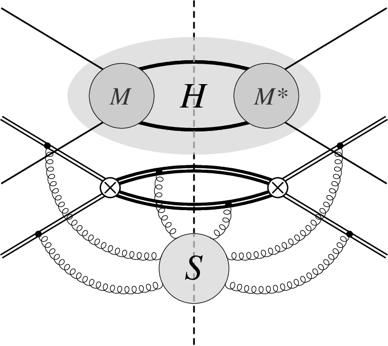
The choice of a basis for the color structures in the factorization formula is crucial. Indeed, if the hard matrix elements are decomposed into singlet and octet configurations of the final state, then the out-going Wilson lines of the soft functions at threshold, i.e. having the same velocity, can be combined into one as shown in A. The summation in Eq. (5) becomes diagonal [7], since the color configurations of the singlet and octet are orthogonal (for initial state gluons, there are two octet configurations, symmetric and anti-symmetric - they are also orthogonal by Bose symmetry). The final factorization formula is now
| (6) |
where the single color index in the hard and soft functions specifies diagonal elements of both, and runs over singlet and octet configurations.
At this point, we have to take into account the effect of potential interactions between the non-relativistic final state quarks. Fortunately, it turns out that we do not have to make substantial changes in our exposition [8]. As long as the hard function contains -wave effects only and is decomposed into irreducible color representations of the final state, non-relativistic effects factorize from the soft effects. This factorization implies that the heavy-quark velocity must be set to zero in the soft component, as we already assumed. On the other hand, the hard amplitudes are to be expanded in the velocity, rather than just evaluated at threshold. In principle, we could now further factorize the potential effects in the hard functions as explained in Ref. [8], but we shall not do that, since we are not interested in their resummation, but rather in the fixed order expansion of the cross sections at threshold. This is achieved by formula Eq. (6) after inclusion of the renormalization of the PDFs in the soft limit in order to yield finite results. A last subtlety concerns the restriction to -wave contributions in the hard functions. Indeed, it is to be expected that higher partial waves will occur in the velocity independent terms of their threshold expansions beyond NLO. Nevertheless, they are not enhanced by soft radiation at NNLO and, consequently, do not spoil the expansion generated with Eq. (6).
Although the partonic cross section on the left hand side of Eq. (6) suffers from initial state collinear divergences only, factorization introduces additional divergences into the hard and soft functions on the right hand side. We now consider the renormalization of these infrared divergences of the hard functions. Since the latter are given by total cross section contributions due to color projected purely virtual amplitudes, the information we need is contained in the singularities of the virtual amplitudes themselves. It turns out that the complete divergence structure of a UV renormalized amplitude is encoded in the following equation
| (7) |
where the renormalization constant is a matrix in color space and has a non-trivial dependence on the kinematics , and by the same on the masses of the external partons. It can be derived from the differential equation
| (8) |
where the color space matrix anomalous dimension is given by [24]
| (9) |
Its structure for massless partons has been determined already in Ref. [25]. The structure of the massive case has been studied in Refs. [26, 27], with explicit expressions for the second line given in Refs. [27, 6]. Finally, the third and fourth lines have been determined in Ref. [24] (see also [28]).
The summations in Eq. (9) run over massless (indices ) and massive (indices ) partons, with the notation denoting unordered tuples of different indices. The color operators act on the color indices of the respective partons. If the particle is a gluon carrying a color index , we have , assuming the result has been projected on color index . Similarly, for an outgoing quark (or incoming anti-quark) the generator is , whereas for an incoming quark (or outgoing anti-quark) the generator is . The kinematic dependence is contained in , where the sign factor if the momenta and are both incoming or outgoing, and otherwise. For massive partons there is , , and . The cusp anomalous dimensions, , for the massless and massive cases, and the functions can be found in Ref. [24] and references therein.
It is interesting to note that the triple color correlations given in the third and fourth lines of Eq. (9) cannot contribute to the divergences of spin and color summed amplitudes at NNLO, as long as the Born amplitudes do not contain complex couplings or masses. This implies in particular that they will not contribute to top-quark pair-production amplitudes, which was noticed for the quark annihilation channel in Ref. [6] and for both channels in Ref. [24]. In the general case, the argument is as follows. First, notice that one can decompose the Born amplitude treated as a vector in color and spin space in terms of color structures
| (10) |
where the vectors are made of and only. The amplitudes are stripped of all color factors generated from QCD vertices. Now, for all different (the indices make no distinction this time between massive and massless partons), there is
| (11) |
simply because the operators are hermitian and commute with each other as long as the parton indices are different, and because the structure constants are real. On the other hand, both sides of Eq. (11) are real, since they can be evaluated with the Cvitanović algorithm [29] containing only real expressions. The color matrix elements of the triple color correlator are thus anti-symmetric in the color indices and we have
| (12) | |||||
Since , the right hand side of Eq. (12) vanishes if is real. Due to elementary spin summation rules, this is the case if there are no complex parameters in the Lagrangian (the case of complex parameters is generally of interest, since we might want to describe unstable particles).
The argument presented above is, of course, also valid for diagonal matrix elements between color projected Born amplitudes, which shows that the NNLO renormalization constants for our hard functions can be determined from the dipole correlations given in the first two lines of Eq. (9). Since the initial partons are either in the fundamental, or the adjoint representation, while the final state may be in a singlet or octet configuration, we have to consider a set of color vectors , where denotes the representation of the initial partons, while that of the final state. The subscripts and in the latter case stand for symmetric and anti-symmetric octets in the case of an initial configuration. The bare hard functions for heavy flavor production are given by
| (13) |
where the right hand side is expanded in the heavy-quark velocity, , up to and including terms of order . denotes the product of the flux, and color and spin average factors, while are the purely virtual UV renormalized amplitudes for heavy flavor production, where the initial state is specified by the color representation . The expansion in in the definition of the hard functions would directly correspond to the soft approximation of taking the matrix element at threshold and keeping the exact phase space, if there were no potential effects. Due to the latter, the result contains inverse powers and logarithms of .
The renormalization of the hard functions is now achieved with
| (14) |
where the renormalization constant satisfies the equation
| (15) |
with
| (16) |
Contrary to the hard function itself, the hard anomalous dimensions are finite in the limit, and do not depend on the scattering angle . They can be found in B.
We mentioned before that the same formalism can be applied to the production of a fundamental object, e.g. a color octet scalar. Clearly, the constant will also be used for the renormalization of the soft function, which does not depend on the nature of the final state. This means that the latter does not play any role in the divergences of the amplitude at threshold. Indeed, this is true for the real part of the anomalous dimension (the imaginary part contains Coulomb phases). The final state anomalous dimension coefficients in Eq. (9) for massive states have a purely soft origin.
3 Soft function
We define the bare soft function for color octet production at rest as follows
| (17) | |||||
where the summation in the first line is taken over all possible states with energy , and in the second line over color indices. The Wilson line operators discussed in A have directions , for the two incoming light-cone states, and for the outgoing octet at rest. Notice that time ordering is in fact only necessary for the product of the two incoming lines. The notation specifies the representation of the initial states as and , and the restriction to the hard scattering color structure corresponding to the irreducible component of the tensor product . We consider three cases
| (18) |
where , and the symmetric tensor is defined through . The invariance of the color structures together with the gauge transformation properties of the Wilson lines, Eq. (49), assure the gauge invariance of the soft function.
Up to NNLO, the singularities in of are known to only depend on the Casimir invariants of the representations of the Wilson lines [6, 7]. We have checked explicitly that this is valid for the exact dependence as well. Since the out-going massive Wilson line is always in the octet representation, the result depends on only through . Therefore, we will drop the subscript in in all the subsequent formulae.
The prefactor in Eq. (17) and the normalization of the color structures in Eq. (18) guarantee that the soft function reduces to at leading order. Dimensional analysis allows to write the following perturbative expansion
| (19) |
where the coefficients depend on , color (through and ) and the number of light quark flavors (as usual, through ).
We now apply a Mellin transform
| (20) |
where and . We only keep the leading behavior in , since the limit in Mellin space corresponds to the soft limit . The last line of the above equation demonstrates that the soft function depends on rather than separately on and . The finiteness of the partonic cross section implies that the renormalized soft function is given by
| (21) |
where we have suppressed the dependence on the initial state parton in both and , the latter being the renormalization constant of the parton distribution function. satisfies the equation
| (22) |
where is the soft expansion of the Altarelli–Parisi splitting kernel in Mellin space, which can be found in B. In consequence, the soft function obeys the Renormalization Group Equation (RGE)
| (23) |
which shows that the logarithmic dependence on in and on in must combine into a dependence on their product as given in . This is a demonstration of the well known fact that the singular part of the soft limit of the splitting kernels is given by the same soft anomalous dimension, which governs the soft-collinear singularities of the virtual amplitudes.
The RGE Eq. (23) can be used to resum large logarithms of . For this purpose, it is sufficient to evolve from the scale , where is small, to the actual scale . We are, however, concerned with the fixed order perturbative expansion, and will now present the calculation and results at NNLO.
3.1 Calculation up to
The contribution to the soft function for color octet production at threshold has been obtained in [15, 6], and for general representations of the three Wilson lines in [7]. With the conventions of Eq. (19), the result reads
| (24) |
The contribution is conveniently evaluated in the momentum representation, where Wilson lines become eikonal lines. Each emission of a gluon with momentum from a hard parton with momentum contributes a factor
| (25) |
where is the sum of and the momenta of the gluons emitted before for an in-going line (minus sign in the denominator), or after for an out-going line (plus sign in the denominator). The phase space integrations are performed with
| (26) |
for the real-virtual (one-loop corrections to single gluon emission), and double-real (double-gluon or quark-anti-quark emission) cases respectively. For a gluon pair in the final state, an additional factor of has to be included.
Our result for the bare contribution in -dimensions is presented in the form of four contributions
| (27) |
The first three of them correspond to double-real radiation, whereas the last one to the real-virtual corrections. The two cases are discussed separately.
3.2 Double-real corrections

|

|

| |
| (A) | |||

|

|

| |
| (B) |

|

|

|
| (C) |

|

|

|
The complete set of double-real emission graphs is depicted in Fig. 2. We have divided the diagrams into three categories: (A) two emissions from eikonal lines, (B) gluon splitting after emission from an eikonal line, (C) massless quark-pair emission. The division into (A) and (B) is not gauge invariant. In order to uniquely define the contributions of the interferences between the (A) and (B) categories, we mention that we work in the Feynman gauge and that we take the gluon polarization sums to be
| (28) |
In consequence, we also have to take ghost pairs into account, when evaluating the square of the sum of the diagrams from (B).
In our calculation, we have not made use of non-abelian exponentiation [30, 31] (see, however, next subsection for an application in the real-virtual case). The color factors are obtained for and subsequently translated into Casimir operators. The occurring phase space integrals can be evaluated analytically by the following method. After canceling numerators with denominators where possible, partial fractioning is used to obtain denominators with the smallest number of different scalar products from the set , , , where and are the momenta of the emitted gluons. Scalar products of the gluon momenta with are harmless, since they only depend on the gluon energy. Subsequently, the denominators involving , are split with a Mellin-Barnes representation
| (29) |
where the contour is chosen to separate the poles of the gamma functions. The angular integrations can be performed with the following formulae [32]
| (30) |
The energy integrations in the resulting integrals can be performed directly in terms of the Euler beta function
| (31) |
After application of the Barnes’ lemmas, we end up with at most one-fold Mellin-Barnes integrals, which can be resummed to hypergeometric functions by closing contours and taking residues. In practice, we have used the packages MB [33] and HypExp [34] for the manipulation of Mellin-Barnes integrals and hypergeometric functions respectively.

The results are given separately for three parts. The first part corresponds to the square of category (A) from Fig. 2. The result contains a single hypergeometric function, due to the interference diagrams shown in Fig. 3. We obtain
| (32) |
The second part, due to the interference of categories (A) and (B) is the most complicated. The result contains several hypergeometric functions 11 1 A subset of the graphs evaluated here occurs in the case of singlet production, i.e. for the soft function for the Drell–Yan process given in [14]. The result from [14] contains an Appell function, which can be expressed in terms of a hypergeometric function: .
| (33) |
The third part is given by the sum of the squares of categories (B) and (C). It is particularly simple, because it can be thought of as the contribution with an insertion of the imaginary part of the gluon vacuum polarization on the gluon line. The result reads
| (34) |
3.3 Real-virtual corrections
Let us now consider virtual corrections to the soft function. Since we are working in dimensional regularization, a Feynman integral does not vanish if the result of the integration can be represented in the form
| (35) |
where and are some real constants with , is a dimensionful parameter, and the proportionality coefficient does not contain any other dimensionful parameters with dependent exponents. In the case of purely virtual corrections involving external eikonal lines only, the result must have integer scaling with respect to all the available momentum parameters. This implies the vanishing of , since the denominators of the Feynman integrands contain no other dimensionful parameters. In consequence, purely virtual corrections vanish.
Non-vanishing contributions are obtained once at least one real particle, a gluon, is emitted, as for the real-virtual corrections we wish to discuss in this subsection. In this case, we have two possible types of dimensionful parameters, which are invariant under hard momentum rescaling, and can thus be used in place of above
| (36) |
where is the momentum of the external gluon, while with , and are the momenta of the eikonal lines.
We can now consider two different types of emissions: from an eikonal line, or from a virtual gluon line. In the case of an emission from an eikonal line, the denominators of the Feynman integrands depend on the emitted gluon momentum through only, with , and the momenta of the emitting eikonal line, the emitted gluon, and the loop integration respectively. Therefore, the result of the integration depends non-trivially only on (ignoring the numerator, which does not influence the -dimensional scaling of dimensionful parameters), and thus either on or , where is the momentum of the other eikonal line integrated in the loop (if the integration involves two different eikonal lines). Such emissions will thus only give non-vanishing contributions, if either or . Emissions from gluon lines give non-vanishing contributions either if the loop contains two different eikonal lines, in which case the result can be expressed through , or if the single eikonal line in the loop is massive, in which case the result is expressed through . The possible graphs generated according to these considerations are shown in Fig. 4.
 |
 |
 |
 |
 |
 |
 |
 |
 |
 |
 |
 |
 |
 |
||

The pairs of graphs in boxes in Fig. 4 can be combined using color algebra and eikonal identities. This is a simple case of eikonal exponentiation [30, 31] for multiple eikonal lines joined at one point. Consider for example the two graphs of Fig. 5. The color factor of the right graph can be represented as the sum of the color factor of the left graph and an additional contribution
| (37) |
If we ignore the second term on the right hand side of this equation, the two graphs will only differ in the kinematics. Their sum can then be written under the same integral sign and will contain the factor
| (38) |
This is the basic eikonal identity, which shows that the two emissions can be completely factorized. Such a contribution corresponds to a product of a real emission and a pure virtual contribution. It thus vanishes by the arguments from the beginning of this subsection. In consequence, for each pair of emissions as in Fig. 5, it is sufficient to only consider the second graph with a modified color factor corresponding to the second term on the right hand side of Eq. (37).
As far as the virtual integrals are concerned, it turns out that they are the same as those that were calculated in [35]. The complete list is
| : | , | , | |
|---|---|---|---|
| : | , | , | , |
| : | , | , |
where the naming of the master integrals, , and , matches that of Ref. [35]. Our integrals are all integrated to Euler gamma functions in -dimensions, because we only have one massive line.
The remaining phase space integration has the same complexity as in the case. We use a subset of the formulae from the calculation of the double-real corrections, but never have to introduce any Mellin-Barnes integrations. Therefore, the final result does not contain any hypergeometric functions and is given by
| (39) |
3.4 Renormalized result
After summing the contributions from the previous subsections and renormalizing according to Eq. (21), we obtain the following perturbative expansion of the soft function for color octet production at threshold in Mellin space
| (40) |
with
| (41) |
In case the initial state is a color octet as well, i.e. , this result further simplifies to become
| (42) |
Of course, the logarithmic terms proportional to , , in these expressions can be derived directly from the RGE Eq. (23). The new results are thus at .
4 Conclusions and outlook
We have presented the result for the next-to-next-to-leading order soft function for color octet production at threshold. The primary use of this result is the derivation of the constants in the threshold expansion of NNLO QCD cross section for heavy-flavor pair-production. This will be one of the topics covered in an upcoming publication.
Our results may have further applications, for example in the determination of threshold expansions of NNLO cross sections for other massive particle (e.g. squarks, gluinos) production in pairs, or as single fundamental states (e.g. color octet scalars). Essential is only the combined color configuration of the final state. The results could also be generalized to arbitrary representations, since the most complicated part of the calculation was the evaluation of the integrals. We have refrained from such a generalization in this publication.
Since the result for the bare soft function is exact in -dimensions, it can be used as part of a calculation of the soft function at higher orders.
Acknowledgments
This research was supported by the German Research Foundation (DFG) via the Sonderforschungsbereich/Transregio SFB/TR-9 “Computational Particle Physics”. The work of M.C. was supported by the DFG Heisenberg programme.
Appendix A Wilson lines and their properties
We consider the following Wilson line operator
| (43) |
which represents the contribution to the path integral of a classical particle charged under the representation of the gauge group, and moving in a straight line with four-momentum between the points and . The operator acts in color space, with in front of the exponential denoting path ordering. This allows to account for the color state evolution of the particle due to gluon emission. Finally, stands for the bare coupling constant. The relation between the bare and renormalized couplings is given at the level of as
| (44) |
The renormalization constant can be determined using the scale independence of and the renormalization group equation satisfied by
| (45) |
with , .
In our exposition we do not need the shift, , of the trajectory, and often explicitly write the color indices. Therefore, we introduce the following simplified notation
| (46) |
The gauge group representations relevant to this study are: 3 for quarks, for anti-quarks, and 8 for gluons. For these three cases, there is
| (47) |
Notice that
| (48) |
because the hermitian conjugation implies the same change of the order of the color operators in the path ordering, as the different definition of the operators in Eq. (47), while the field operators commute. Gauge transformation properties of Green functions involving Wilson lines can be verified using covariance
| (49) |
where is the gauge transformation matrix at point in the representation .
The Wilson line operator satisfies a first order linear differential equation
| (50) |
where the second equation is the boundary condition. This leads to the composition law
| (51) |
which implies a differential equation on the second argument of the operator
| (52) |
which we shall use below. Since the operator acting on the right hand side of the differential equation, Eq. (50), is anti-hermitian, is unitary.
We restrict ourselves to Wilson lines for a straight line motion, because they model soft gluon emission from a hard emitter, the kinematics of which is not affected by the radiation. In momentum space, soft radiation is described by eikonal lines, where each emission contributes a kinematical factor , with and the hard and soft momenta respectively. This factor is rescaling invariant in the hard momentum, a property which the Wilson line must, therefore, also have. This can only be realized if the arguments of are restricted to null or infinity, i.e. . Our lines are semi-infinite, i.e. start or end at 0, where the hard process takes place in the semi-classical picture of the collision. In this case, the integration in the exponent in the definition Eq. (43) is regulated by a factor , with , and sign as appropriate to make the integral convergent. These factors correctly reproduce the causal prescription in the eikonal propagators in momentum space.
Let us now consider the case of an out-going heavy-quark–anti-quark pair at threshold. The quarks share the same four-momentum , where we have used rescaling invariance to rescale the energy to unity. It has been shown in [7] that as long as the pair is in an irreducible representation of the gauge group, the eikonal lines can be combined into one. We reproduce here the argument in our notation for the singlet and octet cases.
For a singlet initial configuration after the production in the hard process, the soft radiation is described by
| (53) |
which in fact means that there is no soft radiation from the final state. In the case of an octet configuration we have to consider the combination
| (54) |
We wish to prove that this combination can be replaced by a single line in the octet representation. This is equivalent to the statement
| (55) |
at . The equation is trivially satisfied at . It is also satisfied at all , because both sides fulfill the same differential equation obtained by taking a derivative in and using Eq. (52).
Appendix B Anomalous dimensions
Here we give the anomalous dimensions necessary to determine the renormalization constants for the hard functions. In the octet case, they have been originally determined in Refs. [6, 7]
| (56) |
Notice that the anomalous dimension for the adjoint representation of the initial state, i.e. for gluon fusion, is the same for the symmetric and anti-symmetric final state color octet configuration.
Additionally, we reproduce the necessary soft limits of the splitting functions in Mellin space, which are, up to this order, textbook material
| (57) |
where and . As is well known, the off-diagonal terms of the splitting functions are not singular in the soft limit.
References
References
- [1] P. Bärnreuther, M. Czakon and A. Mitov, Phys. Rev. Lett. 109 (2012) 132001 [arXiv:1204.5201 [hep-ph]].
- [2] M. Czakon and A. Mitov, JHEP 1212 (2012) 054 [arXiv:1207.0236 [hep-ph]].
- [3] M. Czakon and A. Mitov, JHEP 1301 (2013) 080 [arXiv:1210.6832 [hep-ph]].
- [4] M. Czakon, P. Fiedler and A. Mitov, Phys. Rev. Lett. 110 (2013) 252004 [arXiv:1303.6254 [hep-ph]].
- [5] M. Beneke, M. Czakon, P. Falgari, A. Mitov and C. Schwinn, Phys. Lett. B 690 (2010) 483 [arXiv:0911.5166 [hep-ph]].
- [6] M. Czakon, A. Mitov and G. F. Sterman, Phys. Rev. D 80 (2009) 074017 [arXiv:0907.1790 [hep-ph]].
- [7] M. Beneke, P. Falgari and C. Schwinn, Nucl. Phys. B 828 (2010) 69 [arXiv:0907.1443 [hep-ph]].
- [8] M. Beneke, P. Falgari and C. Schwinn, Nucl. Phys. B 842 (2011) 414 [arXiv:1007.5414 [hep-ph]].
- [9] M. Cacciari, M. Czakon, M. Mangano, A. Mitov and P. Nason, Phys. Lett. B 710 (2012) 612 [arXiv:1111.5869 [hep-ph]].
- [10] M. Beneke, P. Falgari, S. Klein and C. Schwinn, Nucl. Phys. B 855 (2012) 695 [arXiv:1109.1536 [hep-ph]].
- [11] M. Beneke, P. Falgari, S. Klein, J. Piclum, C. Schwinn, M. Ubiali and F. Yan, JHEP 1207 (2012) 194 [arXiv:1206.2454 [hep-ph]].
- [12] M. Czakon and A. Mitov, Nucl. Phys. B 824 (2010) 111 [arXiv:0811.4119 [hep-ph]].
- [13] M. Czakon and A. Mitov, Phys. Lett. B 680 (2009) 154 [arXiv:0812.0353 [hep-ph]].
- [14] A. V. Belitsky, Phys. Lett. B 442 (1998) 307 [hep-ph/9808389].
- [15] A. Idilbi, C. Kim and T. Mehen, Phys. Rev. D 79 (2009) 114016 [arXiv:0903.3668 [hep-ph]].
- [16] A. Ferroglia, B. D. Pecjak and L. L. Yang, Phys. Rev. D 86 (2012) 034010 [arXiv:1205.3662 [hep-ph]].
- [17] A. Ferroglia, B. D. Pecjak, L. L. Yang, B. D. Pecjak and L. L. Yang, JHEP 1210 (2012) 180 [arXiv:1207.4798 [hep-ph]].
- [18] A. Ferroglia, B. D. Pecjak and L. L. Yang, JHEP 1309, 032 (2013) [arXiv:1306.1537 [hep-ph]].
- [19] A. Ferroglia, S. Marzani, B. D. Pecjak and L. L. Yang, arXiv:1310.3836 [hep-ph].
- [20] H. X. Zhu, C. S. Li, H. T. Li, D. Y. Shao and L. L. Yang, Phys. Rev. Lett. 110 (2013) 082001 [arXiv:1208.5774 [hep-ph]].
- [21] H. T. Li, C. S. Li, D. Y. Shao, L. L. Yang and H. X. Zhu, Phys. Rev. D 88 (2013) 074004 [arXiv:1307.2464 [hep-ph]].
- [22] V. Ahrens, A. Ferroglia, M. Neubert, B. D. Pecjak and L. -L. Yang, JHEP 1109 (2011) 070 [arXiv:1103.0550 [hep-ph]].
- [23] N. Kidonakis, Phys. Rev. D 82 (2010) 114030 [arXiv:1009.4935 [hep-ph]].
- [24] A. Ferroglia, M. Neubert, B. D. Pecjak and L. L. Yang, JHEP 0911 (2009) 062 [arXiv:0908.3676 [hep-ph]].
- [25] S. M. Aybat, L. J. Dixon and G. F. Sterman, Phys. Rev. D 74 (2006) 074004 [hep-ph/0607309].
- [26] A. Mitov, G. F. Sterman and I. Sung, Phys. Rev. D 79 (2009) 094015 [arXiv:0903.3241 [hep-ph]].
- [27] T. Becher and M. Neubert, Phys. Rev. D 79 (2009) 125004 [Erratum-ibid. D 80 (2009) 109901] [arXiv:0904.1021 [hep-ph]].
- [28] A. Mitov, G. F. Sterman and I. Sung, Phys. Rev. D 82 (2010) 034020 [arXiv:1005.4646 [hep-ph]].
- [29] P. Cvitanovic, Phys. Rev. D 14 (1976) 1536.
- [30] A. Mitov, G. Sterman and I. Sung, Phys. Rev. D 82 (2010) 096010 [arXiv:1008.0099 [hep-ph]].
- [31] E. Gardi, J. M. Smillie and C. D. White, JHEP 1306 (2013) 088 [arXiv:1304.7040 [hep-ph]].
- [32] G. Somogyi, J. Math. Phys. 52 (2011) 083501 [arXiv:1101.3557 [hep-ph]].
- [33] M. Czakon, Comput. Phys. Commun. 175 (2006) 559 [hep-ph/0511200].
- [34] T. Huber and D. Maitre, Comput. Phys. Commun. 175 (2006) 122 [hep-ph/0507094].
- [35] I. Bierenbaum, M. Czakon and A. Mitov, Nucl. Phys. B 856 (2012) 228 [arXiv:1107.4384 [hep-ph]].