How do we imagine the cosmic expansion? Usually this is a traditional image used in popular science, as well as in textbooks and even monographs. This is a “bird’s-eye view” or a “god’s view”, when we find ourselves out of our space observing it from outside. For example, we imagine an inflating ball, or a stretching surface, which represent our expanding universe. More than that, it is convenient to imagine all points on this ball (or the surface) visible similtaniously, i.e. we see the whole picture “as it is now”. Hence, we not only observe the universe “from outside”, but also “see” all its points at the same time.

This is a useful image (maybe, it is necessary for understanding), however, a real observer never sees such a picture, it is impossible in principle. How the expansion would look like for an “internal” observer?

Let us imagine that we can make observations with arbitrarily high precision, or that we can observe long enough to measure with existing instruments changes in parameters of distant sources due to their recession. How can we better illustrate the results presenting the cosmic expansion? Or, let our goal be a realistic 3D model (for example, for a planetarium) of the picture that an observer sees in an expanding universe. Which parameters fit better for such a task? In particular, which velocity we have to choose to illustrate recession of galaxies?

In this methodological note we demonstrate that one of the best choice is the velocity related to the so-called angular distance, $d_{\Theta}$. We discuss some characteristics of this parameter, and show how it behaves in different universes. This approach, in our opinion, is an important supplement to the traditional illustration (“god’s view”), and helps to form a more adequate image of an expanding universe. This is essential, as many phenomena in cosmology are not vivid and, at first glance, contradict common sense (which includes a very advanced “common sense”, see for example an interesting discussion about feasibility of superluminal velocities of the Hubble flow and different corresponding misconception and mistakes in [1], and also in [2] and references therein). Insufficient clarity of cosmic phenomena results, for example among students, in difficulties in qualitative understanding of the expansion of the universe and associated effects. This is what we hope to overcome.

Definitions and properties of different distance measures used in cosmology can be found in any standard textbook on cosmology (see, for example, [3]). In the present section we review basics of several main definitions of cosmological distances as we extensively use some of them below.

Let us consider a Friedmann universe. In this space we can make a special choice of time coordinate for which all surfaces of constant time are homogenious (this defines the cosmic time). It is natural to use it in future considerations.

The flat Friedmann metric has the usual form:

Here $t$ is cosmic time. It is worth noting that cosmic time is not directly available to an “internal” observer who sees the universe as inhomogenious (the farther — the denser). The second term in the equation represents the Hubble flow — distant objects recede due to increasing scale factor $a$, while their comoving coordinates do not change.

As for comoving coordinates, it is natural to introduce a spherical system with an observer at the origin. Then distances and velocities defined below depend only on the radial comoving coordinate $\chi$. We will consider universes filled with a one-component perfect fluid, in this case all necessary formulae can be obtained in explicit (and rather simple) form. Indeed, for the equation of state we have:

where $p$ is pressure, $\rho$ is matter density, and $c$ is the speed of light. The homogenious solution for the time evolution of the scale factor is $a\sim t^{1/\alpha}$, where $\alpha=3(w+1)/2$. As the Hubble parameter $H=\dot{a}/a=1/(\alpha t)$ and $t\propto a^{\alpha}$, we can, using the definition of the redshift $1+z(t)=a(t_{0})/a(t)$, (where $a(t_{0})$ is the scale factor at the present time), express the Hubble parameter in terms of the redshift: $H=H_{0}(1+z)^{\alpha}$ ($H_{0}$ is its present value).

Using the light propagation equation $ds^{2}=0$, the comoving coordinate of the object observable now at some redshift $z$ can be obtained in a standard way for a given equation of state parameter $\alpha$:

where the observer is conveniently located at $\chi=0$. For models with $\alpha>1$, corresponding to decelerating universes, the integral converges as $z\to\infty$. It is well known that this indicates the existence of the particle horizon (particles with larger $\chi$ can not be observed at the present moment). For $\alpha<1$ the particle horizon does not exist, and the event horizon appears with the comoving coordinate:

This is the coordinate which light emitted now (from $\chi=0$) will reach in the infinite future. Correspondingly, events which at present (according to cosmic time) occur on objects with $\chi>\chi_{\mathrm{e.h.}}$ will never be seen by the observer located at the origin of the coordinate system.

It is instructive to compare how an object crosses the event horizon in an accelerating universe with the same process in black holes (where one can define time at spatial infinity and time on a free falling object, but there is no special time for the picture “as a whole”, i.e. no analogue of the cosmic time). Looking at the universe from “god’s point of view” it is possible to “see” the event horizon at $\chi=\chi_{\mathrm{e.h.}}$, and claim, for example, that: “If the $\Lambda$CDM-model with the currently accepted values of cosmological parameters is true, then galaxies with $z>1.8$ are beyond the event horizon,” – the statement which is absolutely impossible in a description of free fall into a black hole.

A real cosmological observer has no access to the whole picture of the universe at the cosmic time “now”, and the coordinate $\chi=\chi_{\mathrm{e.h.}}$ has no special meaning for him/her. In this sense, the analogue of the infinite (from the position of a distant observer) process $r\to r_{\mathrm{g}}$ of free fall into a black hole is the infinite process $z\to\infty$ seen by a cosmological observer. Of course, the above-mentioned claim has a well-defined meaning without any reference to the cosmic time “now” if we “exchange” the observer and the source. Namely, it means that any light emitted by us now will never reach the galaxy at $\chi=\chi_{\mathrm{e.h.}}$. (for more details, see [10, 11]).

Now we address definitions of two different distance measures. One is valid in the “god’s perspective”, another is connected to the “observer’s perspective”.

The proper distance is defined as $d=a\chi$. If we are interested in distances for $t=t_{0}$ (at the same moment of cosmic time for all sources) the scale factor in the equation should be equal to its present day value $a(t_{0})$. To obtain the proper distance at the moment of light emission we need the scale factor at that time $a(t_{\mathrm{em}})$.

The general formula for the proper distance at the present moment, $t_{0}$, is the following:

This distance is useful in order to imagine the general structure of the universe we live in. It grows monotonically with increasing redshift, tending to a finite value if $z\to\infty$ for $\alpha>1$. This gives us an intuitively clear picture of a finite distance to the particle horizon.

In what follows, we will mostly consider another possiblity, which is related to the picture which an observer can really see. The proper distance to an object at the moment of light emission, $d(t_{\mathrm{em}})$, coincides with the well-known (and sometimes directly observable) angular distance, $d_{\Theta}$, defined as $d_{\Theta}=D/\delta$, where $D$ is the diameter of an emitter, and $\delta$ is its observed angular diameter.

For a perfect fluid with parameter $\alpha$ we have:

In contrast to the present day proper distance (i.e., distance “now”), the dependence of the angular distance on the redshift is not monotonic for most realistic cosmological models (if we do not consider some exotics, only in de Sitter model with $\alpha=0$ the function $d_{\Theta}(z)$ has no local maximum). For example, for a dust-dominated universe ($p=0$, so $\alpha=3/2$) $d_{\Theta}$ reaches its maximum at $z=5/4$ which is well within the currently observable universe. That is why it may be hard to believe that this quantity is the most relevant characteristic of the distance. However, from the point of view of observations it is exactly what we need. Remember, for example, the observational proof that our universe is close to the flat one, which is based on calculations of the angular distance to the surface of last scattering. It is true (though it may sound strange) that spots on the last scattering surface ($z\sim 1100$) seen in the CMB temperature maps were situated (at the time of emission) at the same distance (about 13 Mpc) as some near-by galaxy with $z\approx 0.003$ (of course, the moment of emission for this galaxy was much later with respect to cosmic time). ¹¹ 1 It is convenient to use on-line cosmological calculators for such estimates, for example, the one by Ned Wright http://www.astro.ucla.edu/$\sim$wright/CosmoCalc.html.

As light trajectories in a flat universe are straight lines (see Fig. 1), the fact that angular size of distant objects grows with growing redshift has just this reason — objects with larger redshifts were at the time of emission closer to us than objects with lower redshifts (for $z$ large enough). Of course, if we use $z$ itself to describe how distant an object is from us (as it often happens), such situation does not occur. However, if our goal is to introduce a meaningful measure of distance in the picture directly seen by an observer, it is the angular distance that plays this role.

In the final part of this section we briefly remind definitions of several other cosmological distances.

The photometric distance is rather popular in observational cosmology. It is defined as:

where $L$ is the luminosity of an object, $f$ is the observed flux. Note, that the photometric distance diverges at the event horizon (if it exists in the model). However, this is because of the energy dilution due to redshift encoded in the definition of this parameter.

The proper motion distance is rather interesting because it formally coinsides with the proper distance for the present moment: $d_{\mathrm{pm}}=a(t_{0})\chi$. Currently there are no effective methods to determine this distance. In principle, they can appear in connection to studies of jets in distant sources.

It should be noted that the popularity of photometric distance in contemporary observational cosmology is related to the existence of “standard candles”, but not to some special role of this distance in theoretical models. The angular distance is currently not so popular, however, the situation may change with appearence of a “standard ruler”. Some time ago it was proposed to use a characteristic distance scale of barionic acoustic oscillation for this purpose [5]. This proposal have been already used in a several studies [6, 7, 8]. These authors used data on hundreds of thousands of galaxies and quasars to estimate basic cosmological parameters.

We would like to underline once again that a special role of the angular distance, in our opinion, is not related to the quality of currently available astrophysical data, but follows from the fact that this distance coincides with the fundamental theoretical quantity — proper distance at the moment of emission.

Different distances are related to each other as follows:

Before we address the problem of definition of the velocity characterizing the Hubble flow, it is necessary to note that the existence of different velocities with different meanings is rather typical in the General relativity. A classical example of this situation is the description of free fall into a black hole. From the point of view of an observer at spatial infinity the motion of falling objects is initially accelerated, then, after reaching its maximum the coordinate velocity (which in the case of free fall from infinity with zero initial velocity is equal to $2c/[3/\sqrt{3}$]) is decreasing [9]. It is clear that this coordinate velocity defined as the ratio of distance to the time interval measured at the infinity is important only for description of an observed picture of free fall. It is useless when we describe processes in the vicinity of the black hole itself. Our goal is to find an analogue for such velocity in the case of the Hubble flow.

Usually the velocity of the Hubble flow is defined as:

because the corresponding comoving coordinate does not change (we ignore pecular velocities, so $\dot{\chi}=0$).

Using equations from the previous section, it is easy to see that for the universe filled with a perfect fluid the velocity “now” is:

while the velocity at the moment of emission is:

We now remind a reader some properties of these two velocities. Some other interesting details can be found in [12].

It can be easily seen that for a decelerating universe ($\alpha>1$) the velocity at the moment of emission diverges as $z\to\infty$ (which is natural, because the time derivative of the scale factor is not bounded near the Big Bang). On the contrary, for an accelerating universe this velocity for $z\to\infty$ tends to a finite value larger than $c$ (except the de Sitter solution, where this limit is exactly $c$).

What is more interesting is the asymptotic behavior of the velocity “now” for $z\to\infty$. The limiting value can be either bigger or smaller than $c$, depending on the particular cosmological model. ²² 2 When speaking about the speed of light we mean its local value of $c\approx 300000$ km s^-1. If a galaxy recedes from us superluminously, the photon emitted “to the exterior” will recede from us with even larger velocity, moving with respect to the galaxy with the speed of light $c$.

The boundary case occures for $w=1/3$ ($\alpha=2$, radiation dominated universe). For this case $H=H_{0}(1+z)^{2}$, and, correspondingly, $v_{\mathrm{em}}=cz$, $v_{\mathrm{now}}=cz/(1+z)$. This means, that $v_{\mathrm{now}}$ tends to $c$ for $z\to\infty$. For a matter dominated universe ($w=0$, $\alpha=3/2$), $v_{\mathrm{now}}$ tends to $2c$, while $v_{\mathrm{now}}=c$ is reached at a finite $z$ (this is the Hubble sphere, $R_{\mathrm{c}}=c/H$). On the contrary, if $w=1$ ($\alpha=3$), then $v_{\mathrm{now}}(z=\infty)=c/2$, so the velocity now does not reach $c$ for any $z$ (the Hubble sphere is located beyond the particle horizon). The general formula for this limit at $z\rightarrow\infty$ as a function of the parameter $\alpha$ is very simple: $v_{\mathrm{now}}(z=\infty)=c/(\alpha-1)$. This formula cannot be applied for $\alpha<1$ because a finite limit of this velocity does not exist, and it diverges with diverging $z$.

It is clear that the velocity “now” corresponds to the “god’s perspective”, as it is necessary to see the whole universe at the same moment of cosmic time. What about the velocity at the moment of emission, does it correspond to the “observer’s view”? When we remember that cosmic time is used for derivation of this velocity, we understand that the answer is “no”. The reason is: light signals emitted by an observed object during some time interval with respect to cosmic time will be detected by an observer during longer time interval measured by the observer’s clock, leading to smaller that $v_{\mathrm{em}}$ observed velocity. As a result, $v_{\mathrm{em}}$ also corresponds to the “god’s perspective, so a “god”, being a time traveller and observing the whole universe at the time of emission, can see the observer and the observed object receding from each other with a relative velocity equal to $v_{\mathrm{em}}$. So, the question is: what a real observer can see?

Such kind of problem (when we totally neglect the existence of cosmic time and consider only observable values) begins to be practically important due to a possibility to detect time variation of redshifts (due to recession) in the near future. Corresponding formula for the redshift change measured by an observer’s clock gives [13]:

If we also take into account that $\dot{H}/H^{2}=-\alpha$, we obtain for the observable time derivative of the proper distance at the moment of emission the following estimate:

This velocity which is supposed to represent the velocity of the Hubble flow directly measured by an observer, does not generally coincide with any of velocities discussed above. The velocity at the moment of emission (defined with respect to cosmic time) differs from it by factor $(1+z)$ which represents the ratio of time intervals at the object at the moment of emission $dt_{1}$ and at the observer’s location when he/she receives the signal $dt_{2}=(1+z)dt_{1}$. As this velocity is, by definition, the rate of change of angular distance, we will denote it as $v_{\Theta}\equiv\tilde{v}_{\mathrm{em}}$.

The value of $v_{\Theta}$ has absolutely different asymtotics for large $z$. First of all, it is easy to see that it vanishes for $z\to\infty$ having a maximum at some finite $z$ if the model has the event horizon ($\alpha<1$). In particular, its maximum for de Sitter model is equal to $c/4$ and occurs at $z=1$. If the model has the particle horizon, the situation is more complicated. Again, suddenly, the radiation-dominated universe appears to be a special one. For $w<1/3$ this velocity behaves as in the model with the event horizon, having a maximum at finite $z$. This maximum disappears for $w=1/3$ (the velocity monotonically increases up to the value $c$, reaching it at the particle horizon). For stiffer equations of state, this velocity has no upper limit and diverges as $z\to\infty$.

If maximum of $v_{\Theta}$ exists, it is reached at

The location of the maximum increases monotonically with increasing $\alpha$ starting from $z_{\mathrm{m}}=1$ for de Sitter universe and reaching infinity for $w=1/3$, passing through $z_{\mathrm{m}}=3$ for the important case of the dust-dominated universe. As for the maximum value of $v_{\Theta}$ itself, it increases from $c/4$ (de Sitter) up to $c$ (radiation-dominated universe), passing through $c/2$ for the dust-dominated universe. The case of $\alpha=1$ should be considered separately. For such universe (the Miln model) the scale factor grows linearly in time, the velocities $v_{\mathrm{em}}$ and $v_{\mathrm{now}}$ are equal to each other, and $v_{\Theta}$ reaches a maximum equal to $c/e$ at $1+z_{\mathrm{m}}=e$, where $e$ is the famous Euler number.

It is interesting that about 50 years ago such a velocity could pretend to be a measure of the Hubble flow which is always subluminal, reaching $c$ only at the particle horizon in the limit of ultrarelativistic equation of state of the matter filling the universe. This equation of state have been considered as the stiffest for a physically reasonable matter in, for example, Landau-Lifshitz course of theoretical physics. Even now, the only “non-exotic” matter with stiffer equation of state is a massless scalar field — the object, strictly speaking, still existing only theoretically. However, keeping in mind that superluminal recession velocities are allowed, as well as the fact that the equation of state $p=\rho/3$ is not a limiting case in contemporary physics, we do not insist that above-mensioned asymptotics of the velocity $v_{\Theta}$ have some deep meaning.

In Figs. 2-5 three velocities described above are shown as functions of the redshift for several cosmologically interesting equations of state.

In the de Sitter model ($\alpha=0$) the universe accelerates, so the velocity at the moment of emission, $v_{\mathrm{em}}$, is always smaller than the present day velocity, $v_{\mathrm{now}}$ (Fig. 2). As it was mensioned above, the former tends to $c$ for $z\to\infty$, the latter is unbounded from above passing $c$ at $z=1$. As for the velocity with respect to an observer, $v_{\Theta}$, it reaches the maximum value $c/4$ at $z=1$, and for larger $z$ decreases tending to zero.

Dust-dominated universe always decelerates, that is why $v_{\mathrm{em}}>v_{\mathrm{now}}$ (Fig. 3). The former velocity is unbounded from above, the latter has the asymptotic value equal to $2c$ at the particle horizon. The observable velocity $v_{\Theta}$ reaches the value of $c/2$ at $z=3$, and than decreases. We can see also that $v_{\mathrm{now}}=c$ at the same $z=3$. From the explicit formulae of this section it is clear that this is not a coincidence. Namely, in a one-component Friedmann model with a perfect fluid $v_{\mathrm{now}}=c$ at the same $z$ as the redshift corresponding to the maximum value of $v_{\Theta}$ (it happens when $(1+z)^{1-\alpha}=2-\alpha$).

The case of the radiation-dominated universe ($\alpha=2$) is a special one (Fig. 4). It corresponds to the smallest $\alpha$ for which $v_{\Theta}$ has no maximum as a function of $z$. Moreover, for this universe $v_{\mathrm{now}}$ and $v_{\Theta}$ are equal to each other (both are equal to $cz/(1+z)$). As for $v_{\mathrm{em}}$, it becomes superluminal for $z$ larger than unity, having extremely simple expression $v_{\mathrm{em}}=cz$.

As a curious fact, a reader can look at a funny “symmetry” in the definition of the velocities under discussion if we change $\alpha\to 2-\alpha$.

Finally, in the universe filled with the maximally stiff fluid (Fig. 5) both $v_{\mathrm{em}}$ and $v_{\Theta}$ monothonically grow to infinity with increasing $z$. As for the velocity “now”, it always remains subluminal.

Obviously, our proposal of the best candidate for an observable velocity of the Hubble flow is not free from limitations. From the very beginning we use the concept of the proper distance which is not an observable quantity. To define it in a strict way it is necessary to have a chain of observers each of which in a given moment measures distance to a neighbour, and after all measurements are summed up. Realization of such a “project” is even out of the area of sci-fi, so we have to find an other way round. Instead, we use coincidence between the proper distance at the moment of emission (we consider this quantity to be the most meaningful in the visible picture because an observer really “sees” the object, but not calculates its position) with the angular distance, which potentially can be measured. So, in some sense we can state that the proper distance at the moment of emission can be measured by an observer. In this picture, if we want to speak about some “visible velocity of the universe expansion”, $v_{\Theta}$ is the most meaningful characteristic of the visible velocity of the Hubble flow.

Of course, the existence of an illustrative picture is not a necessary condition to work on many problems. For example, most often authors in their studies use just a redshift as a measure of distance. This is enough to perform calculations. Due to this many scientists assume that vast discussions of numerous velocities and distances used in cosmology is superfluous and can be a reason of embarrassment. For example, in [1] one can find the statement (though not supported by the author) that the recession velocity is an unphysical quantity as it cannot be measured directly. Still, in our opinion, the existence of distinct images with clear physical meaning allows to use intuition in a study. Observable quantities which represent important aspects of cosmological models deserve scrutinous analysis.

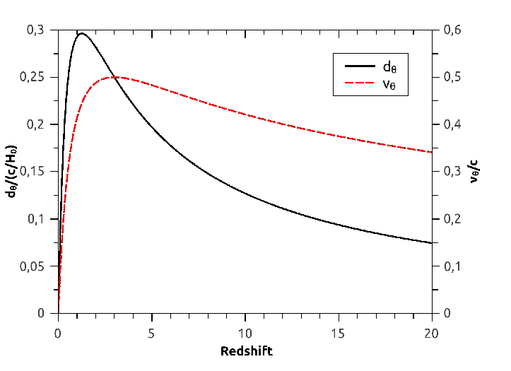
It is interesting to discuss how position of maxima for the angular distance and velocity change as functions of the redshift. Maximum of the velocity in different cases can appear on larger or smaller $z$ in comparison with the maximum of the angular distance (see Fig.6 which is plotted for the dust dominated universe). However, the general feature is: in accelerating universes the velocity maximum appears on smaller redshifts than the maximum of the angular distance, in decelerating universes the situation is opposite. The transitional case corresponds to the Miln universe with $a\sim t$; in this case both maxima coinside at $z=e-1\approx 1.71$. It is interesting to note, that the maximum of the angular distance appears when $v_{\mathrm{em}}=c$ (for a single-fluid universe this happens at $(1+z)^{\alpha-1}=\alpha$, see Fig. 1).

Notice, that changes in the angular distance correspond to our phychological perception of an object receding from us. Subjectively we say that the object becomes more distant when its size diminishes, and of course, we mean angular size. Due to this, if one makes a realistic visualization of the universe expansion as viewed by an observer on Earth it is necessary to reproduce, in the first place, changes of angular distances.

Let the universe in our visualization (imagine it on the dome of a planetarium) be filled (up to, say, $z\sim 10$) with identical galaxies of the same size. We see more distant galaxies as weak redden sources. Angular size behaves according to Fig. 6: starting from some distance farther sources look larger (they have smaller angular distance). In dynamic, we would see that galaxies become redder and dimmer. However, the main effect of recession would be visible due to diminishing angular sizes of all galaxies. The rate of this diminishing of the angular size would also go down (see Fig. 6 and a sketch in Fig. 7). It is essential that according to an intuitive idea of a horizon, the dynamic would “freeze” for the most distant sources.

As for the prospects of direct detection of dynamic of expansion, the first results can be obtained due to $\dot{z}$ measurements with ultrastable spectrographs on large telescopes of the next generation (see a review in [13]). Besides that, there are some hopes that GAIA can detect decrease of sizes of gravitationally bound systems due to cosmic expansion [14].

Expecting direct observational measurements of time variations of quantities characterizing the Hubble expansion, it is useful to remind which parameters are observable directly and which, — being important for understanding and illustration of the expansion, — represent just a theoretical construction. This was the main goal of this note.

In brief, our discussion can be summarized as follows:

• •

  We want to define quantities which fit the best to our intuitive understanding of visible distance and velocity of the Hubble flow in an expanding universe.

• •

  Proper distance is a fundamental quantity of the theory and does not depend on our observational abilities and current astrophysical knowledge.

• •

  We see an object as it was at the moment of emission, so it is natural to consider the distance at the moment of emission as an important characteristic of the source.

• •

  Proper distance at the moment of emission can be calculated in the same way as the angular distance. In addition, the angular distance and its derivative correspond to our psychological perception of receding and to intuitive expectations about the behavior of objects on the horizon. Therefore, just angular distance and its derivative (in time) are the most natural characteristics of the Hubble flow from the observer’s point of view.

References

- [1] Murdoch H S Quat. J. R. Astron. Soc. 18, 242 (1977)
- [2] Davis T M, Lineweaver C H, Webb J K American J. Phys. 71 358 (2003)
- [3] Weinberg S Gravitation and cosmology (John Wiley and sons, 1972)
- [4] Coles P, Lucchini F Cosmology. The origin and evolution of cosmic structure (John Wiley and sons, 2002)
- [5] Basset B, Hlozek R in: Dark Energy: Observational and Theoretical Approaches, Ed. Ruiz-Lapuente P, (Cambridge, UK, Cambridge University Press, 2010) arXiv: 0910.5224
- [6] Percival W J et al. Mon. Not. R. Astron. Soc. 401, 2148 (2010)
- [7] Blake C et al. Mon. Not. R. Astron. Soc. 415, 2892 (2011)
- [8] Busca N G et al. Astron Astrophys. 552, id. A96 (2013)
- [9] Blinnikov S I, Vysotsky M I, Okun L B Phys. Usp. 46, A04 (2003)
- [10] Starobinsky A.A. Gravitation and Cosmology, 6, 157 (2000).
- [11] Sahni V. and Starobinsky A.A. Int. Journ. Mod. Phys., D9, 373 (2000).
- [12] Davis T M, Lineweaver C H Publ. Astron. Soc. Australia 21 97 (2004)
- [13] Quercellini C, Amendola L, Balbi A, Cabella P, Quartin M Phys. Rep. 521 95 (2012)
- [14] Darling J Astrophys. J. Lett. in press, arXiv: 1310.0500 (2013)