Hydrodynamic Limits and Propagation of Chaos for Interacting Random Walks in Domains
Abstract
A new non-conservative stochastic reaction-diffusion system in which two families of random walks in two adjacent domains interact near the interface is introduced and studied in this paper. Such a system can be used to model the transport of positive and negative charges in a solar cell or the population dynamics of two segregated species under competition. We show that in the macroscopic limit, the particle densities converge to the solution of a coupled nonlinear heat equations. For this, we first prove that propagation of chaos holds by establishing the uniqueness of a new BBGKY hierarchy. A local central limit theorem for reflected diffusions in bounded Lipschitz domains is also established as a crucial tool.
1 Introduction
The original motivation of this project is to study the transports of positive and negative charges in solar cells. We model a solar cell by a domain in that is divided into two disjoint sub-domains and by an interface , a -dimensional hypersurface, which can be possibly disconnected. and represent the hybrid medium that confine the positive and the negative charges, respectively. At microscopic level, positive and negative charges are initially modeled by independent reflected Brownian motion (RBM) with drift on and on respectively. (In this paper, they are actually modeled by independent random walks on lattices inside and that serve as discrete approximation of RBM with drifts.) These random motions model the transport of positive (respectively negative) charges under an electric potential (See Figure 1).
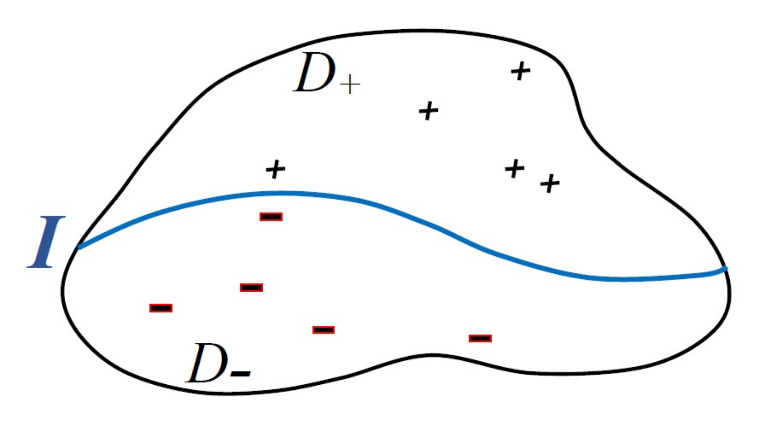
These two types of particles annihilate each other at a certain rate when they come close to each other near the interface . This interaction models the annihilation, trapping, recombination and separation phenomena of the charges. The interaction distance is of microscopic order where is comparable to 1, and the intensity of annihilation per pair is of order where is a given parameter. This means that, intuitively and roughly speaking, according to a random time clock which runs with a speed proportional to the number of pairs (one particle of each type) of distance , we annihilate a pair (picked uniformly among those pairs of distance less than ) with an exponential rate of parameter . The above scaling guarantees that in the limit, a nontrivial proportion of particles are annihilated in any open time interval. We investigate the scaling limit of the empirical distribution of positive and negative charges; that is, the hydrodynamic limit of this interacting diffusion system. We show that in the macroscopic level, the empirical distribution converges to a deterministic measure whose density satisfies a system of partial differential equations that has non-linear interaction at the interface.
The study of hydrodynamic limits of particle systems with stochastic dynamics is of fundamental importance in many areas. This study dates back to the sixth Hilbert problem in year 1900, which concerns the mathematical treatment of the axioms of physics, and to Boltzmann’s work on principles of mechanics. Proving hydrodynamic limits corresponds to establishing the law of large number for the empirical measure of some attributes (such as position, genetic type, spin type, etc.) of the individuals in the systems. It contributes to our better understanding of the asymptotic behavior of many phenomena, such as chemical reactions [31], population dynamics [20, 32, 34], super-conductivity [40], quantum dynamics [21], fluid dynamics [24], etc. It reveals fascinating connections between the microscopic stochastic systems and deterministic partial differential equations that describe the macroscopic pictures. It also provides approximations via stochastic models to some partial differential equations that are hard or impossible to solve directly.
Since the work of Boltzmann and Hilbert, there have been many different lines of research on stochastic particle systems. Various models were constructed and different techniques were developed to establish hydrodynamic limits. Among those techniques, the entropy method [25] and the relative entropy method [40] are considered to be general methods. Unfortunately these methods do not seem to work for our model due to the singular interaction near the interface.
Many models studied in literature are conservative, for example exclusion processes [27, 28] and Fleming-Viot type systems [8, 9]. Reaction-diffusion systems (R-D system) constitute a class of models that are typically non-conservative. These are systems which have hydrodynamic limits of the form (a reaction-diffusion equation, or R-D equation in short), where is a function in which is thought of as the reaction term. R-D systems arise from many different contexts and have been studied by many authors. For instance, for the case is a polynomial in , these systems contain the Schlögl’s model and were studied in [18, 19, 29, 30] on a cube with Neumann boundary conditions, and in [4, 5] on a periodic lattice. Recently, perturbations of the voter models which contain the Lotka-Volterra systems are considered in [14]. In addition to results on hydrodynamic limit, [14] also established general conditions for the existence of non-trivial stationary measures and for extinction of the particles.
Our model is a non-conservative stochastic particle system which consists of two types of particles. In [9], Burdzy and Quastel studied an annihilating-branching system of two types of particles, for which the total number of particles of each type remains constant over the time. Its hydrodynamic limit is described by a linear heat equation with zero average temperature. In contrast, besides being non-conservative, our model gives rise to a system of nonlinear differential equations that seems to be new. Moreover, the interaction between two types of particles is singular near the interface of the two media, which gives rise to a boundary integral term in the hydrodynamic limit. The approach of this paper provides some new tools that are potentially useful for the study of other non-equilibrium systems.
We now give some more details on the discrete approximation of the spatial motions in our modeling. We approximate by square lattices of side length , and then approximate reflected diffusions on by continuous time random walks (CTRWs) on . The rigorous formulation of the particle system is captured by the operator in (2.8).
Let be the position of the particle with index in at time . We prescribe each particle a mass and consider the normalized empirical measures
Here stands for the Dirac measure concentrated at the point , while if and only if the particle is alive at time , and if and only if the particle is alive at time . For fixed positive integer and , is a random measure on . We want to study the asymptotic behavior, when (or equivalently ), of the evolution in time of the pair .
1.1 Main results
Our first main result (Theorem 2.20) implies the following. Suppose each particle in is approximating a RBM with gradient drift , where is strictly positive. Then under appropriate assumptions on the initial configuration , the normalized empirical measure converges in distribution to a deterministic measure
for all , where is the solution of the following coupled heat equations:
| (1.1) |
and
| (1.2) |
where is the inward unit normal vector field on of and is the indicator function on . Note that corresponds to the particular case when there is no drift.
The above result tells us that for any fixed time , the probability distribution of a randomly picked particle in at time is close to when is large, where is a normalizing constant. In fact, the above convergence holds at the level of the path space. That is, the full trajectory (and hence the joint law at different times) of the particle profile converges to the deterministic scaling limit described by (1.1) and (1.2), not only its distribution at a given time.
Question: How about the limiting joint distribution of more than one particles ?
Our second main result (Theorem 2.22) answers this question. It asserts that propagation of chaos holds true for our system; that is, when the number of particles tends to infinity, their positions appear to be independent of each other. More precisely, suppose and unlabeled particles in and , respectively, are chosen uniformly among the living particles at time . Then, as , the probability joint density function for their positions converges to
uniformly for and for in any compact time interval, where is a normalizing constant.
1.2 Key ideas
A key step in our proof of propagation of chaos (Theorem 2.22) is Theorem 3.7. The latter establishes uniqueness of solution for the infinite system of equations satisfied by the correlation functions of the particles in the limit . Such infinite system of equations is sometimes called BBGKY-hierarchy in statistical physics. Our BBGKY hierarchy involves boundary terms on the interface, which is new to the literature. Our proof of uniqueness involves a representation and manipulations of the hierarchy in terms of trees. This technique is related to but different from that in [21] which used Feynman diagrams. It is potentially useful in the study of other stochastic models involving coupled differential equations.
To establish hydrodynamic limit result (Theorem 2.20), we employ the classical tightness plus finite dimensional distribution approach. Tightness of in the Skorokhod space is proved in Theorem 4.4. This together with the propagation of chaos result (Theorem 2.22) establishes the hydrodynamic limit of the interacting random walks.
Two new tools for discrete approximation of random walks in domains are developed in this article. Namely, the local central limit theorem (local CLT) for reflected random walk on bounded Lipschitz domains (Theorem 2.12) and the ‘discrete surface measure’ (Lemma 2.4). We believe these tools are potentially useful in many discrete schemes which involve reflected Brownian motions.
Weak convergence of simple random walk on to RBM has been established for general bounded domains in [6] and [7]. However, we need more for our model; namely a local convergence result which guarantees that the convergence rate is uniform up to the boundary. For this, we establish the local CLT. We further generalize the weak convergence result and the local limit theorem to deal with RBMs with gradient drift. There are two reasons for us to consider gradient drift. First, it is physically natural to assume the particles are subject to an electric potential. Second, the maximal extension theorem, [13, Theorem 6.6.9], which is a crucial technical tool used in [6] and [7], has established only in symmetric setting. The proof of the local CLT is based on a ‘discrete relative isoperimetric inequality’ (Theorem 5.5) which leads to the Poincaré inequality and the Nash inequality. The crucial point is that these two inequalities are uniform in (scaling of lattice size) and is invariant under the dilation of the domain .
The paper is organized as follows. In section 2, we introduce the stochastic model and some preliminary facts that will be used later. We then prove the existence and uniqueness of solution for the coupled PDE. The main results, Theorem 2.20 and Theorem 2.22, will be rigorously formulated. We also mention various extensions of our main results in Remark 2.25. Section 3 and section 4 contains the proof of Theorem 2.22 and Theorem 2.20 respectively. Section 5 is devoted to the proofs of the discrete relative isoperimetric inequality and the local CLT.
2 Notations and Preliminaries
For the reader’s convenience, we list our notations here:
| set of all integers | |
| positive integers | |
| non-negative integers | |
| set of all real numbers | |
| Borel measurable functions on | |
| bounded Borel measurable functions on | |
| non-negative Borel measurable functions on | |
| continuous functions on | |
| bounded continuous functions on | |
| non-negative continuous functions on | |
| continuous functions on with compact support | |
| space of paths from to | |
| equipped with the Skorokhod metric | |
| -dimensional Hausdorff measure | |
| space of finite non-negative Borel measures on | |
| equipped with the weak topology | |
| (or ) | |
| number of living particles at at time | |
| process with generator in Definition 2.8 | |
| and | independent processes with generator |
| , state space of | |
| , the normalized empirical measure in | |
| , the state space of | |
| filtration induced by the process , i.e. | |
| indicator function at or the Dirac measure at | |
| (depending on the context) | |
| weak convergence of random variables (or processes) | |
| positive constants | |
| ‘-point approximation’ of constructed in Lemma 2.4 | |
| ‘discrete surface measure’ constructed in Lemma 2.4 |
| Process | Semigroup | Heat kernel | Measure | Generator | State space |
|---|---|---|---|---|---|
where in the above,
We also use the following abbreviations:
| a.s. | almost surely |
| LDCT | Lebesque dominated convergence theorem |
| CTRW | continuous time random walk |
| RBM | reflected Brownian motion |
| local CLT | local central limit theorem |
| LHS | left hand side |
| RHS | right hand side |
| WLOG | without loss of generality |
Definition 2.1.
A Borel subset of is called -rectifiable if is a countable union of Lipschitz images of bounded subsets of with (As usual, we ignore sets of measure 0). Here denotes the -dimensional Hausdorff measure.
Definition 2.2.
A bounded Lipschitz domain is a bounded connected open set such that for any , there exits such that is represented by for some coordinate system centered at and a Lipschitz function with Lipschitz constant , where does not depend on and is called the Lipschitz constant of .
Assumption 2.3.
are given adjacent bounded Lipschitz domains in such that is a finite union of disjoint connected -rectifiable sets, are given functions which are strictly positive, is a fixed parameter.
2.1 Interacting random walks in domains
In this subsection, we describe the interacting random walk model. We start with some key ingredients needed in discrete approximation.
2.1.1 Discrete approximation of surface measure
To capture the boundary behavior of our processes near the interface in the discrete scheme, we need a discrete approximation of the surface measure on . The construction of and in the following lemma is a key to our approximation scheme. For us, denotes the set of non-negative integers.
Lemma 2.4.
Suppose is a bounded Lipschitz domain of . Let be closed, connected and -rectifiable. Let for . Then there exist finite subsets of and functions such that (a) and (b) below hold simultaneously:
- (a)
(2.1) where denotes the number of elements in the finite set , is the ball with radius centered at , and is a constant that depends only on .
- (b)
For any equi-continuous and uniformly bounded family ,
(2.2)
Proof We can always split into small pieces. The point is to guarantee that each piece is not too small, so that and that (2.1) holds. Since is -rectifiable, we have
for , where does not depend on . Since is closed, it is regular with dimension in the terminology of section 1 of [16]. Hence by [15] or section 2 of [16], we can build “dyadic cubes” for . More precisely, there exists a family of partitions of into “cubes” such that
- (i)
if , and , then either or ;
- (ii)
if , then
- (iii)
for all and .
Here the constant is independent of or . Note that is the surface measure of and that property (iii) tells us that the cubes have relatively small boundary. In particular, (iii) implies for all cube .
Suppose . We pick one point from each to form the set . Finally, we define . It follows from (ii) that for some which depends only on . The inequality (2.1) follows from and the Lipschitz property of . It remains to check (2.2).
Fix any . There exists such that whenever . Hence for large enough (depending only on ),
The desired convergence (2.2) now follows. ∎
Remark 2.5.
(2.2) implies that we have the weak convergence on the space of positive finite measure Borel measures on . Here is the dirac delta measure at , and is the surface measure restricted to . (2.1) is a control on the number of points locally in . We call the ‘-point approximation’ of and the ‘discrete surface measure’ associated to . ∎
Remark 2.6.
The above lemma remains true if is the finite union of disjoint closed connected and -rectifiable subsets of . This enables us to deal with disconnected interface . ∎
2.1.2 Reflected diffusion and random walk approximation
We now describe the motion of each underlying particle. First we fix a bounded Lipschitz domain and any . Without loss of generality, we assume that the origin . Let be the union of all closed line segments joining nearest neighbors in , and the connected component of that contains the point . Set . We can view as the vertices of a graph whose edges coming from . We also denote the graph-boundary , where is the degree of in .
Suppose is strictly positive. Define
Since is Lipschitz, is a regular Dirichlet form on and so there is a -symmetric diffusion associated with it (cf. for example [12]).
Definition 2.7.
We call the -reflected diffusion, where is the identity matrix. When , is called the reflected Brownian motion (RBM) in . Hence a -reflected diffusion is a RBM in with drift .
The -infinitesimal generator of is
Moreover, has the Skorokhod representation:
| (2.3) |
where is the inward unit normal of and is the positive continuous additive function (PCAF) of whose Revuz measure is (c.f.[12]). We call the boundary local time of .
Next, we define to be a continuous time random walk (CTRW) on with exponential waiting time of parameter and one step transition probabilities
where are symmetric weights (conductances) to be constructed in two steps as follows: First, for every and , define
| (2.4) | |||||
| (2.5) |
Clearly, for all . Note that since is and strictly positive on , when is sufficiently small, and are strictly positive for every and . Second, we define
Now for all . A heuristic reason of the above construction can be found in [23].
We call the -approximation of . Clearly, is symmetric with respect to the measure defined by
Since , there exists a constant such that
| (2.6) |
Moreover, whenever converges to .
A special but important case is when . In this case, is simply the reflected Brownian motion on , and is a simple random walk on the graph . It is proved in [6] that converges weakly to the reflected Brownian motion as .
Recall that by Assumption 2.3, we are given . We denote by a -reflected diffusion in , and by the -approximation of .
2.1.3 Random walks with interaction
Fix () and such that . Assume there are “+” particles in and “” particles in at . Each particle moves as an independent CTRW (see the previous subsection) in its respective domain . Let be the finite subset of defined in Lemma 2.4. For each , pick an and an which are closest to (See Figure 2). A pair of particles of opposite charges at is being killed with a certain rate to be explained. Note that for small enough, we have , where is the Lipschitz constant of .

The state space of the particle system is the collection of configurations
| (2.7) |
The state of the particle system at time is a random element . Here stands for the number of particles at at time . We omit and for convenience when there is no ambiguity. For example, we write and in place of and respectively. The function such that and for is denoted as .
Definition 2.8.
is defined to be the unique strong Markov process which has the generator given by
| (2.8) |
where is the generator of two families of independent random walks in and , respectively, with no annihilation between them, namely
| (2.9) | |||||
and is the operator corresponding to annihilation between particles of opposite signs at the interface , namely
| (2.10) |
where is the one-step transition probabilities for the CTRW on (without any interaction) and
| (2.11) |
with and being constructed by Lemma 2.4.
The expression for comes from the underlying assumptions of the model: First, the term is combinatorial in nature. Since there are pairs of particles at position , the chance of killing is proportional to the number of ways of selecting a pair of particles near the interface. Second, each pair of particles near disappears at rate where is a parameter. Intuitively, in the limit, the amount of annihilation in a neighborhood of a point is proportional to the surface area of the interface in that neighborhood. The scaling is suggested by the observation that there are about ”layers” starting from the interface , so that the chance for a particle to arrive near is of order . is comparable to 1 and can be viewed as a normalizing constant with respect to the lattice. This choice (2.11) is justified in the proof of Theorem 3.5.
2.2 Discrete heat kernel
Throughout this subsection, is a bounded Lipschitz domain in , is strictly positive, is a -reflected diffusion. It is well known (cf. [1, 26] and the references therein) that has a transition density with respect to the symmetrizing measure (i.e., and ), that is locally Hölder continuous and hence , and that we have the followings: there are constants and such that
| (2.12) |
for every . Using (2.12) and the Lipschitz assumption for the boundary, we can check that
| (2.13) |
| (2.14) |
where are constants which depends only on , and .
On other hand, suppose . Then for and ,
| (2.15) |
Now let be the -approximation of with symmetrizing measure . The transition density of with respect to the measure is
| (2.16) |
Clearly, is strictly positive and is symmetric in and .
We will prove in Section 5 that enjoys two-sided Gaussian bound and is jointly Hölder continuous uniform in for some , and that converges to uniformly on compact subsets of . In rigorous terms, we have the following three results. The important point is that the constants involved in these results do not depend on .
Theorem 2.9.
(Gaussian upper bound) There exist , , and such that for every and ,
| (2.17) |
and
| (2.18) |
Theorem 2.10.
(Gaussian lower bound) There exist , , and such that for every and ,
| (2.19) |
Theorem 2.11.
(Hölder continuity) There exist positive constants , and such that for all , we have
| (2.20) |
Theorem 2.12.
(Local CLT)
for any compact interval .
To establish the tightness of , we need the following uniform estimate for the heat kernel of CTRW on near the boundary of . It is the discrete analog of (2.14).
Lemma 2.13.
There exist and such that
| (2.21) |
for all and . Here is the graph-boundary of , which is all the vertices in with degree less than .
Proof Fix . By the Gaussian upper bound in Theorem 2.9, we have
Here are all constants which depend only on , and . Note that in the second last line, we used the fact that , which follows from Lemma 2.4. The proof is now complete. ∎
In general, we use for quantities related to . For example, , and denote the generator, semigroup and transition density of the reflected diffusion in with respect to . In addition, we use for quantities related to the CTRWs in the discrete domains . For example, denotes the transition density of the CTRW on with respect to the measure . We also denote for .
By applying Lemma 2.13 to , then by the boundedness of in (2.11), Theorem 2.12, Lemma 2.4 and LDCT, we have the following approximation for the local time of on .
Proposition 2.14.
(Discrete local time)
| (2.22) |
2.3 Hydrodynamic limit: system of nonlinear PDEs
In this subsection, we provide suitable notion of solutions for the coupled PDE (1.1) and (1.2), and then prove the existence and uniqueness of the solution. Throughout this subsection, is a bounded Lipschitz domain, is strictly positive, is a -reflected diffusion, and are the semigroup and the transition density of , with respect to the measure .
Observe that (1.1) is a second order parabolic equation for with Robin boundary condition, and (1.2) is a similar equation for . This leads us to consider the following Robin boundary problem, where .
| (2.23) |
By Itó’s formula and the Skorokhod representation for , we see that a classical solution of (2.23), should it exists, has the probabilistic representation
| (2.24) |
where is the boundary local time of .
First we show that the function defined by (2.24) is continuous.
Lemma 2.16.
Suppose , and is defined by (2.24). Then . Moreover, if , then .
Proof Observe that for any ,
By Markov property, the first term is
Since has the strong Feller property (see [1]) and is bounded, is continuous on for any fixed and .
The second term of (2.3) converges to 0 uniformly on , as . This is because its absolute value is bounded by
Hence, is continuous in .
By a similar calculation as in (2.3), we have
Hence,
Both terms go to 0 uniformly in as goes to 0. (In fact, the first term goes to 0 uniformly since the semigroup is strongly continuous on . For the second term, also goes to 0 uniformly in .) Hence is continuous in uniformly in . Therefore, . If , we can extend the above argument to show that . ∎
Remark 2.17.
In fact, one can allow to be unbounded and show that the conclusion of Lemma 2.16 remains true if satisfies a Kato class condition:
∎
Proposition 2.18.
Suppose and . Then
is the unique element in that satisfies the following integral equation:
| (2.26) |
Proof By Lemma 2.16, lies in . Moreover, by Markov property and (2.15) we have
Hence satisfies the integral equation. It remains to prove uniqueness. Suppose also satisfies the integral equation. Then solves
| (2.27) |
By a Gronwall type argument and (2.14), we can show that . More precisely, let . Then
Note that
Combining the above two inequalities, we have
Integrating both sides with respect to on the interval , we have
From this we have on , where is small enough so that . Let , we can show that
and repeat the argument to obtain on (i.e. on ). Inductively, we obtain on . ∎
Now we come to our coupled equation.
Proposition 2.19.
For , consider the Banach space with norm . Suppose and . Then there is a unique element which satisfies the coupled integral equation
| (2.28) |
Moreover, satisfies
| (2.29) |
where is the boundary local time of on the interface .
Functions satisfying equation (2.28) will be called a weak solution of (1.1) and (1.2), as it can be shown that they are weakly differentiable and solve the equations in the distributional sense.
Proof of Proposition 2.19. Define the operator on by , where
Lemma 2.16 implies that maps into . Moreover, for ,
A similar result holds for . Hence,
for some when is small enough.
Hence there is a such that is a contraction map. By Banach fixed point theorem, there is a unique element such that . By Proposition 2.18, is the unique weak solution to the coupled PDE on .
Repeat the above argument, with replaced by , and replaced by . We see that, since , and are the same, we can extend the solution of the coupled PDE uniquely to . Iterating the argument, we have for any , the coupled PDE has a unique weak solution in . Invoke Proposition 2.18 once more, we obtain the desired implicit probabilistic representation (2.29).
2.4 Main results (rigorous statements)
In this paper, we always assume the scaling holds, so that the interacting random walk model is parameterized by a single parameter which is the initial number of particles in each of and . More precisely, for each fixed , we set and let be a Markov process having generator defined in (2.8) and having initial distribution satisfies . We define the empirical measures
It is clear that is a continuous time Markov process (inheriting from that of ) with state space
where denotes the space of non-negative Borel measures on with mass at most 1. is a closed subset of , where the latter denotes the space of finite non-negative Borel measures on equipped with the following metric:
| (2.30) |
where is any countable dense subset of . The topology induced by this metric is equivalent to the weak topology (i.e. if and only if for all ). Under this metric, is a complete separable metric space, hence so are and the Skorokhod space (see e.g. Theorem 3.5.6 of [22]). Here is our first main result.
Theorem 2.20.
(Hydrodynamic Limit) Suppose Assumption 2.3 holds and the sequence of initial configurations satisfies the following conditions:
- (i)
in , where . (Note that has unit mass for all .)
- (ii)
Then for any , as along the sequence , we have
where is the deterministic element in such that
for all , and is the unique weak solution of the coupled PDEs (1.1) and (1.2) with initial value .
Theorem 2.20 gives the limiting probability distribution of one particle randomly picked in at time . This is the -particle distribution in the terminology of statistical physics.
Question: What is the limiting joint distribution of more than one particles?
Before stating the answer, we need to introduce a standard tool in the study of stochastic particle systems: the notion of correlation functions11 1 More precisely, we will be using correlation functions for unlabeled particles. We refer the readers to [33] for the relation between labeled and unlabeled correlation functions.. Recall that the state space of is defined in (2.7). We denote by
the set of configurations with and particles in and respectively. We then define in such a way that whenever ,
| (2.31) |
where is the Poisson polynomial22 2 The notation is suggested by the fact that when is a Poisson random variable with mean . of order , namely and for (in particular, for ). Note that is the number of permutations of objects chosen from distinct objects. So is the total number of possible site to site pairings between labeled particles having configuration with a subset of labeled particles having configuration . An alternative representation of (2.31) will be given in (3.5).
Convention: For and , we define to be with .
Definition 2.21.
Let is the law of a process with generator and initial distribution satisfying
| (2.32) |
For all , we define
| (2.33) |
for all , where
| (2.34) |
when . By convention, we also have . Note that depends on the initial configuration of .
Intuitively, suppose we randomly pick and living particles in and respectively at time , then is the joint probability density function for their positions, up to a normalizing constant. Therefore, it is natural that defined by (2.33) is called the -particle correlation function.
The next is our second main result, propagation of chaos, for our system. It says that when the number of particles tends to infinity, they appears to be independent of each other. Mathematically, the correlation function factors out in the limit .
Theorem 2.22.
(Propagation of Chaos) Under the same condition as in Theorem 2.20, for all and any compact interval ,
where is the weak solution of the coupled PDE.
To investigate the intensity of killing near the interface, we define by
| (2.35) | |||||
| (2.36) |
Clearly, , which measures the number of encounters of the two types of particles near . An immediately corollary of Theorem 2.22 is the following, which is what we need to identify the limit of .
Corollary 2.23.
For any fixed and ,
Proof We only need to apply Theorem 2.22 for the cases and . By definition,
Using (2.6) and Lemma 2.4, we get the first two equations via Theorem 2.22. Using (2.6) and the assumption that , we have the last two equations again by Theorem 2.22. ∎
Remark 2.24.
(Conditions on ) The two conditions for the initial configuration in Theorem 2.20 are mild and natural. They are satisfied, for example, when each particle has the same random initial distribution . Condition (ii) guarantees that, asymptotically, there is no ”blow up” of number of particles at any site. More precisely, this technical condition is imposed so that we have
| (2.37) |
The above can be easily checked by comparing with the process that has no annihilation (i.e. has generator ). Alternatively, we can use the comparison result (3.11) to prove (2.37). ∎
Remark 2.25.
(Generalization) We can generalize our results in a number of ways by the same argument. For example, the initial number of particles in and can be different, the condition can be relaxed to where depends on . The annihilation constant can be replaced by a space and time dependent function . The diffusion coefficients in and can be different. The condition “ has mass one for all ” can be replaced by “the mass of is uniformly bounded in ”. More generally, the same method can be extended to deal with similar models with more than two types of particles. ∎
3 Propagation of Chaos
3.1 Duality
The starting point of our analysis is the discrete integral equation for in Lemma 3.2. At the heart of its proof is the dual relation in Lemma 3.1, which says that the two independent processes and of independent ransom walks with no interaction are dual to each other with respect to the function , where . Such kind of dual formula for the whole grid appeared in [5] and in Chapter 15 of [11].
Lemma 3.1.
(Duality for independent processes) Let and be independent continuous time Markov processes on with generator defined in Definition 2.8. Then we have
| (3.1) |
Proof Assume and . Then we have and for all . Without loss of generality, we may assume and as otherwise both sides inside expectations of (3.1) are zero by the definition of .
Denote the map that sends to for any . We first focus on in Step 1 and Step 2 below.
Step 1. For any and , fix some . Then by the definition (2.31) of ,
| (3.2) |
where -tuples consist of distinct positive integers in the set , and denotes the number of elements in the finite set .
Step 2. Denote by the law of the unlabeled process starting from and has generator . Let , and be independent CTRWs in starting from , whose law will be denoted as . Then by (3.2), we have
| (3.3) |
where is the law of . Denote by the transition density of independent CTRWs in . By Chapman-Kolmogorov equation, we have for any ,
Putting this into (3.3), we have
| (3.4) | |||||
where is the expectation corresponding the probability measure under which each coordinate processes of are independent CTRWs with and are independent of .
Step 3. Now we work on . For any and , take . As in step 1, we have
| (3.5) |
where runs over all -tuples consisting of distinct positive integers in the set , and over all -tuples consisting of distinct positive integers in the set .
Denote by the law of the unlabeled process starting from and has generator . Since all processes on are independent of those on , we can proceed as in step 2 (via (3.5)) to obtain
| (3.6) |
where is independent of with , and its components are mutually independent CTRWs on , respectively. The proof is now complete by taking . ∎
We now formulate the discrete integral equations that we need. Recall the definition of from (2.10) and the definition of from (2.33).
Lemma 3.2.
(Discrete integral equation for ) For any , , , non-negative integers and initial distribution , we have
| (3.7) | |||||
where acts on the -variable of .
Let and be the laws of and respectively. (3.1) is equivalent to saying that for any and , we have
| (3.8) |
Taking , we see that (3.8) is in turn equivalent to
| (3.9) |
where and are the transition semigroup of and , respectively, and they act on the and variables in , respectively. Therefore, with acting on the variable, we have
| (3.10) |
Recall that is the configuration process of our interacting system with generator (see Definition 2.8). Fix and consider the function . We have
is a -martingale for . By (3.10) and the fact that , where is the law of starting from , we have
for all and . This is equivalent to the stated equation in the lemma.
∎
It is clear that . Hence, as an immediate consequence of Lemma 3.2, we have the following comparison result:
| (3.11) |
for all and .
3.2 Annihilation near the interface
For any , we let , the element that has only number of particles at , and none elsewhere. Similarly, we denote by . Set , the element that has only number of particles at , number of particles at , and none elsewhere.
Lemma 3.3.
Let be the operator defined in (2.10) and acts on the -variable of . Then
| (3.12) |
Moreover, if , then
| (3.13) | |||||
| (3.14) | |||||
| (3.15) |
3.3 Uniform bound and equi-continuity
We extend to define continuously on while preserving the supremum and the infinmum in each small -cube. We can accomplish this by the interpolation described in [2] or [39], or by a sequence of harmonic extensions along simplexes with increasing dimensions (described in [23]). Recall that the definition of depends on the initial configuration of the interacting random walks (see Definition 2.21), which has the normalization (2.32).
Theorem 3.4.
There exists such that for any , the family of functions is uniformly bounded and equi-continuous on , which is uniform in the initial configuration that satisfies (2.32).
Proof We first prove uniform boundedness. By (3.11) and the Gaussian upper bound in Theorem 2.9, we have
Since the initial distribution has the property that , we have
| (3.16) | |||||
Thus there exist and such that for all , and ,
| (3.17) |
We next show that both terms on the right hand side of (3.7) are equi-continuous. Recall that we can rewrite the equation (3.7) as
where
Now let , and . For the first term,
where we have used (3.16) in the last line. By the uniform Hölder continuity of (see Theorem 5.12 below) and the fact that , we see that is equi-continuous at . For the second term, note that
| (3.18) |
where
In the remaining, we will show that is equi-continuous. We first deal with in (3.18).
As in (3.16), we have
| (3.19) | |||||
On other hand, using (3.11), the Chapman Kolmogorov equation and assumption (ii) for , in this order, we have
| (3.20) |
for large enough , where is a constant.
We have used (3.19) for the second inequality. The last inequality follows from Hölder’s inequality, (2.37) and (3.20). Therefore for any ,
| (3.21) |
for large enough , where is a constant. Hence as , uniformly for , and small enough. Finally, we deal with . For any , we have
By (3.21), we have . By the Hölder continuity of (cf. Theorem 5.12),
where are positive constants. Since is arbitrary, we see that as , uniformly for small enough . Hence is equi-continuous at an arbitrary . ∎
From Theorem 3.4 and a diagonal selection argument, it follows that for any sequence there is a subsequence along which converges on , uniformly on the compacts, to some , for every . Our goal is to show that
We will achieve this by first showing that both and satisfy the same an infinite hierarchy of equations, and then establishing uniqueness of the hierarchy.
3.4 Limiting hierarchy
Note that is a bounded Lipschitz domain in , and that the boundary contains the disjoint union where
| (3.22) | |||||
| (3.23) |
We define the function by . We also denote , where is the transition density of the reflected diffusion on with respect to the measure . We now characterize the subsequential limits of :
Theorem 3.5.
Let be a sequence of initial configurations that satisfy (2.32) with , and the conditions of Theorem 2.20; that is, their corresponding empirical measures converges weakly to in for some and
| (3.24) |
Denote by the correlation functions for the interacting random walks with initial configuration . Let be any subsequential limit (as ) of . Then the following infinite system of hierarchical equations holds:
| (3.25) | |||||
where is the Lebesgue measure on , is the surface measure of and .
Remark 3.6.
-
(i) The equation expresses as an integral in time involving and , thus forming a coupled chain of equations. In statistical physics, it is sometimes called the BBGKY hierarchy33 3 BBGKY stand for N. N. Bogoliubov, Max Born, H. S. Green, J. G. Kirkwood, and J. Yvon, who derived this type of hierarchy of equations in the 1930s and 1940s in a series papers.. It describes the evolution of the limiting -particle correlation functions and hence the dynamics of the particles.
-
(ii) By Proposition 2.15, (3.25) is equivalent to
(3.26) Here is boundary local time of , the symmetric reflected diffusion on corresponding to , and is a function on defined as
Observe that the coordinate processes of consist of independent copies of reflected diffusions in and independent copies of reflected diffusions in .
Proof of Theorem 3.5. Recall that . We can rewrite (3.7) as
| (3.27) | |||||
Fix any , and . By a simple counting argument and condition (3.24) for , we see that the first term in (3.27) equals
which converges to by Theorem 2.12 and assumption (i) for the initial distributions. Here is the probability measure for starting at .
We now prove that the second term in (3.27) tends to as . The integrand with respect to is at most
| (3.28) |
Note that is a subset of
| (3.29) |
and that for fixed and , we further have
Now we restrict the sum over in (3.28) to the subset , where , and are fixed. Moreover, we denote by and by . Then
The second to the last inequality above follows from the bound (see Lemma 2.4) and the uniform upper bound (3.17). Repeat the above argument for the other subsets of and use the fact again (for in (3.29)), we have, for any , (3.28) is of order and hence converges to 0 uniformly for , as . The second term in (3.27) then converges to 0, by (3.21) and LDCT.
For the third term in (3.27), we split the integrand with respect to into three terms corresponding to (3.13), (3.14) and (3.15) respectively. The term corresponding to (3.13) equals
By Theorem 2.12 and Lemma 2.4,
and the convergence is uniform for . Therefore, by applying Theorem 2.12 again, the term corresponding to (3.13) converges to
We repeat the same argument for the term corresponding to (3.14). Moreover, note that the term corresponding to (3.15) will not contribute to the limit as , by the same argument we used for the second term in (3.27). Therefore, the integrand of the second term in (3.27) converges to
The integral for in the third term in (3.27) then converges to the desired quantity, by (3.21) and LDCT. The proof is complete. ∎
3.5 Uniqueness of infinite hierarchy
Uniqueness of BBGKY hierarchy is an important issue in statistical physics. For example, it is a key step in the derivation of the cubic non-linear Schrödinger equation from the quantum dynamics of many body systems obtained in [21]. Our BBGKY hierarchy (3.25) is new to the literature and the proof of its uniqueness involves a representation and manipulations of the hierarchy in terms of trees. The technique is related but different from that in [21], which used the Feynman diagrams.
Note that, by Theorem 3.5, can be extended continuously to . Uniqueness of solution for the hierarchy will be established on a subset of the space
equipped with the product topologies induced by the uniform norm on .
Theorem 3.7.
(Uniqueness of the infinite hierarchy) Given any . Suppose is a solution to the infinite hierarchy (3.25) with zero initial condition (i.e. ) and satisfies for some . Then we have for every .
The remaining of this subsection is devoted to give a proof of this theorem.
Convention in this subsection: will always denote the functions stated in Theorem 3.7. For notational simplicity, we will also assume and . The proof for the general case is the same. we will also drop from the notation .
It is convenient to rewrite the infinite hierarchy (3.25) in a more compact form as
| (3.30) |
where is a measure concentrated on defined as
Here is the surface measure of restricted to . Similarly, is a measure concentrating on defined as
3.5.1 Duhamel tree expansion
We now describe the infinite hierarchy in detail. It is natural and illustrative to represent the infinite hierarchy in terms of a tree structure, with the ‘root’ at the top and the ‘leaves’ at the bottom. Fix two positive integers and . We construct a sequence of finite trees recursively as follows.
- 1.
is the root, with label .
- 2.
is constructed from by attaching new vertices (call them leaves of ) to it. More precisely, we attach new vertices to the root by drawing edges and edges from the root. Those new leaves drawn by the edges are labeled , while those drawn by the edges are labeled . We also label the edges as and (See Figure 3).
- 3.
When , we view each of the leaves of as a ‘root’ (with a new label, being either or ), and then attach new leaves (leaves of ) to it by drawing edges. Hence there are new leaves, coming from new edges and new edges.
- 4.
Having drawn , we construct by attaching new edges and new leaves from each leaf of by the same construction, viewing a leaf of as a ‘root’.

In , the root is connected to each leaf by a unique path formed by the edges. Moreover, such a path passes through a sequence of labels formed by the leaves of (). We denote these labels by . For example, when , and the path is . Then and the path connects the root to a leaf of with label . Note that the label is not one-to-one. For example, .
For mnemonic reason, we use the same notation to denote the collection of paths that connect the root to a leaf in . By induction, the total number of paths (or the total number of leaves) is
| (3.31) |
Iterating (3.30) times gives
| (3.32) | |||||
where (for ) is defined by and . For example, when , and the path is . Then
3.5.2 Telescoping via Chapman-Kolmogorov equation
By (3.31), the right hand side of (3.32) is a sum of terms of multiple integrals. We will apply the bound to each term, and then simplify the integrand using Chapman-Kolmogorov equation.
We demonstrate this for the twelve terms for the case . The twelve terms on the right hand side of (3.32) are
| (3.33) | |||||
The first four terms came from the leftmost leaf of the previous level, we group them together to obtain, for ,
Note the telescoping effect upon using the Chapman-Kolmogorov equation for the middle two terms in the last equality above gives rise to rather than .
We apply (2.14) to obtain
where are positive constants. Repeat the above argument for the remaining eight terms of (3.33), we obtain
| (3.34) |
The key is to visualize the twelve terms on the right as 12 paths of with the edges relabeled. We denote this relabeled tree by (See Figure 4, ignoring the five leaves in at the moment). More precisely, since all twelve terms on the right are of the form , we only need to record the indexes and the sign. For example, the first four terms can be represented by
Each corresponds to and hence it appears twice. In , these four paths are formed by a edge followed by four edges with labels .

In general, we obtain by relabeling the edges of , while keeping the labels for the vertices and the sign for the edges. The relabeling of edges are performed as follows:
- 1.
At level , we assign the number ‘1’ to all the edges connected to the root. Hence we have ‘’ edges and ‘’ edges, rather than the labels and (See Figure 5 for ).
- 2.
At level , consider the set in which we have copies of (hence there are elements in , in which of them are ). Similarly, let in which we have copies of . For an arbitrary leaf of , let be the labels of (the edges of) the path from the root to in , counting with multiplicity. Finally, the collection of new labels of the edges below , denoted by , is chosen in such a way that
Since and (again, counting multiplicity), the cardinalities of the two sides match:
Induction shows that and the choice for is unique. For example, for leaf of , , and . So , which gives the new labels to the edges below ; see Figure 4.

As a further illustration, we continue to ‘grow’ (see Figure 4) by adding suitably labeled edges to leaves of . Precisely, let be a leaf of .
- •
If , then (this is the case for the leftmost leaf, which has label )
- •
If , then (shown in Figure 4).
- •
If , then .
- •
If , then .
- •
If , then .
- •
If , then .
- •
If , then .
For mnemonic reason, we use the same notation to denote the collection of paths from the root to the leaves of . Any such path is represented by the ordered (new) labels of the edges. We now ‘forget’ the sign of the edges and only record the integer labels. For example, the path is replaced by .
Using the hypothesis (of Theorem 3.7) and applying Chapman-Kolmogorov equation to (3.32), and then applying (2.14), we obtain the following lemma by the same argument that we used to obtain (3.34).
Lemma 3.8.
| (3.35) |
where
| (3.36) |
Our goal is to show that for some . This will imply for small enough. Clearly we have
Unfortunately, this crude bound is asymptotically larger than for any .
3.5.3 Comparison with a ‘dominating’ tree
Note that
This is obtained by comparing the labels in with a ‘dominating’ labeling, in which the labels of the edges below every leaf of is (the sign is discarded). This trick enables us to group the terms at each level.
For the general case, let be an arbitrary leaf of . Note that in , each of the integers appears at most twice and the integer appears at most times. We compare with the ‘dominating’ label defined below:
| Level | ||
|---|---|---|
| 1 | ||
| 2 | ||
| 3 | ||
In the last row, if is even, then and ; if is odd, then and .
We can now group the terms in each level as a sum of terms to obtain
In the last term, we have used the observation that when , the smallest element in is at least 2 and so the sum stops before reaching . From this and the simple estimates like
we have derived the following
Lemma 3.9.
| (3.37) |
where
| (3.38) |
3.5.4 Estimating
Our goal in this section is show that for some . Our proof relies on the following recursion formula pointed out to us by David Speyer:
| (3.39) |
We assume (3.39) for now and use it to establish the following lemma. The proof of (3.39) will be given immediately after it.
Lemma 3.10.
is homogeneous in the sense that
| (3.40) |
Moreover,
| (3.41) |
Proof is obvious from (3.39) after a change of variable. Let be the collection of functions satisfying . We can rewrite as
| (3.42) |
This is a sum of terms. When we put , the smallest term is
Hence we have the lower bound . Unfortunately, the largest term is exactly
which grows faster than for any . Hence for the upper bound, we will employ the recursion formula (3.39). We apply the homogeneity to the right hand side of (3.39) to obtain
The integrals are now simple one dimensional and can be evaluated:
| (3.43) |
Since , we have , where is defined by the recursion
with . The generating function of clearly satisfies . We thus see that , where is the Lambert function. By Lagrange inversion Theorem (see Theorem 5.4.2 of [37]), (for ). Hence by comparing coefficients in the series expansion of , we have as desired. ∎
Remark 3.11.
By Stirling’s formula, (where means ). Hence for some . Monte Carlo simulations suggests that . The recursion (3.43) also makes it clear that ’s are all in (polynomials in with rational coefficients) and makes it easy to compute them recursively. This is because is rational if is odd and is a rational multiple of if is even. For example, , and . ∎
We now turn to the proof the recursion formula (3.39) which is restated in the following lemma.
Lemma 3.12.
| (3.44) |
provided that we set .
Proof The proof is based on standard combinatorial methods for working on sums over planar rooted trees (see [37]).
Step 1: Summing over labeled trees. Recall (3.42). There are elements in . We can visualize each of them as a rooted tree with vertex set and a directed edge from to for each . For example, the 6 elements of can be represented by
The trees are drawn so that arrows point upwards and the children of a given vertex are listed from left to right. Note that the second and forth tree of the list are the same up to relabeling the vertices. The idea is to group terms in (3.42) like this together. First, we rewrite (3.42) in terms of trees. Let be the set of ‘decreasing trees’, which are trees whose vertices are labeled by and such that whenever there is an edge . Then
| (3.45) |
Step 2: Summing over unlabeled trees. A planar tree is a rooted unlabeled tree where, for each vertex, the children of that vertex are ordered. We draw a planar tree so that its children are ordered from left to right. Here are the 5 planar rooted trees on 3+1 vertices:
Let be the set of planar rooted trees with vertices. In general, there are (the Catalan number) elements in , see exercise 6.19 in [37]. We now group all the integrals in (3.45) with the same planar tree. For example, two different labeled trees (the second and forth in our list of labeled trees) both give the same unlabeled planar tree (which is the second in the above list). We redraw this unlabeled planar tree below and attach letters to for later use.
The integrands corresponding to the second and forth labeled trees are
They are the same to
once we relabel the variables by the vertices of . That is, for the first term and for the second.
We now go back and keep track of the bounds of integration. In the first integral, they are and, in the second integral, they are . We can group these together as
which is the same as and .
In general, the inequality constraints we have are of two types. First, whenever we have an edge , we get the inequality . Second, if and are children of with to the left of , then . Let be the polytope cut out by these inequalities where is the variable at the root. We have proved
| (3.46) |
Step 3: Grouping terms for which the root has degree . We abbreviate
if has more than one vertex (otherwise ). Then (3.46) translates into
| (3.47) |
Fix an integer and let be a tree whose root has degree . Removing the root leaves behind children, denoted in chronical order by , and planar subtrees having as its root for . Then
Hence, group together the terms where the root has degree , we have
| (3.48) |
Here the summation conditions include that and each different ordering of are considered to be different, where is the number of vertices in . This abbreviation applies whenever appears.
On other hand, we have by applying (3.47) to each below that
| (3.49) | |||||
3.5.5 Proof of uniqueness
4 Hydrodynamic Limits
This section is devoted to the proof of Theorem 2.20. Throughout this section, we assume the conditions of Theorem 2.20 hold.
4.1 Constructing martingales
Since has a finite state space, we know that for all bounded function that is smooth in the first coordinate with , we have two -martingales below:
| (4.1) |
and
| (4.2) |
where is the generator defined in (2.8). See Lemma 5.1 (p.330) of [27] or Proposition 4.1.7 of [22] for a proof. We will use this fact to construct some important martingales in Lemma 4.1 below.
In general, suppose is a CTRW in a finite state space , whose one step transition probability is and mean holding time at is . Its infinitesimal generator of is the discrete operator
The formal adjoint of is defined by
It can be easily checked that
| (4.3) |
We denote by the generator of the CTRW on , respectively, and by the corresponding formal adjoint. In our case, for all . We can check that if , then
| (4.4) |
Lemma 4.1.
For any ,
| (4.5) |
is an -martingale for , where is the measure-valued process defined by (2.35). Moreover, if , then there is a constant independent of so that for every ,
| (4.6) |
Similar statements hold for .
Proof The lemma follows by applying (4.1) and (4.2) to the function
We spell out the details here for completeness. Observe that . Fix , and define to be the function from to which maps to . Then by the definition of in (2.8),
| (4.7) |
Similarly, for , we have
| (4.8) |
Hence, by linearity of , (4.7) and then (4.3), we have
Hence
| (4.9) |
and is an -martingale by (4.1). Next, we compute . Note that
where can be computed explicitly using (2.8). Hence from (4.2), we can check that
where
After taking expectation for , the first term is the last display is of order at most since , while the second term inside the bracket is of order at most , uniformly in , by (2.37). Hence for some . Doob’s maximal inequality then gives (4.6). ∎
Remark 4.2.
From the second term of (4.9), we see that if the parameter of the killing time is of order , then we need to be comparable to 1. ∎
4.2 Tightness
The following simple observation is useful for proving tightness when the transition kernel of the process has a singularity at . It says that we can break down the analysis of the fluctuation of functionals of a process on into two parts. One part is near , and the other is away from where we have a bound for a higher moment. Its proof, which is based on the Prohorov’s theorem, is simple and is omitted (detail can be found in [23]).
Lemma 4.3.
Let be a sequence of real valued processes such that is continuous on a.s., where . Suppose the following holds:
- (i)
There exists such that for any ,
- (ii)
for any .
Then is tight in .
Here is our tightness result for . We need Lemma 4.3 in the proof mainly because we do not know if is finite or not.
Theorem 4.4.
The sequence is relatively compact in and any subsequential limit of the laws of carries on . Moreover, for all ,
are all tight in .
Proof We write in place of for convenience. By Stone-Weierstrass Theorem, is dense in in uniform topology. It suffices to check that is relatively compact in for all (cf. Proposition 1.7 (p.54) of [27]) for this weak tightness criterion). By Prohorov’s theorem (see Theorem 1.3 and remark 1.4 of [27]), is relatively compact in if (1) and (2) below holds:
- (1)
For all and , there exists a compact set such that
- (2)
For all ,
We first check (1). Since is bounded on and for all , we can always take .
To verify (2), since , we only need to focus on . By Lemma 4.1,
| (4.10) |
So we only need to verify (2) with replaced by each of the 3 terms on RHS of the above equation (4.10).
For the first term of (4.10), we apply Lemma 4.3 for the case and . Since , we have
for some constant which only depends only on . Using Lemma 2.13, we have
which is in as a function in . This implies hypothesis (ii) of Lemma 4.3, via the Chebyshev’s inequality. Hypothesis (i) of Lemma 4.3 can be verified easily using the upper bound (3.17) for the correlation function, or by direct comparison to the process without annihilation:
For the third term of (4.10), by Chebyshev’s inequality, Doob’s maximal inequality and Lemma 4.1, we have
We have proved that (2) is satisfied. Hence is relatively compact. Using (2) and the metric of , we can check that any subsequential limit of the laws of concentrates on . ∎
Remark 4.5.
In general, to prove tightness for in , it is NOT enough to prove tightness separately for and in and respectively. (However, the latter condition implies tightness in trivially). See Exercise 22(a) in Chapter 3 of [22]. For example, converges in but not in . The reason is that the two processes can jump at different times ( and ) that become identified in the limit (only one jump at ); this can be avoided if one of the two processes is -tight (i.e. has only continuous limiting values), which is satisfied in our case since and turns out to be both -tight. ∎
4.3 Identifying the limit
Suppose is a subsequential limit of , say the convergence is along the subsequence . By the Skorokhod representation Theorem, the continuity of the limit in and [22, Theorem 3.10.2], there exists a probability space such that
| (4.12) |
Hence we have for any and ,
Combining with Corollary 2.23, we have
Here we have used the simple fact that if , then a.s.
5 Local Central Limit Theorem
Suppose is a bounded Lipschitz domain and is strictly positive. Suppose is a -reflected diffusion and be an -approximation of , described in the subsection 2.1.2. In this section, we prove the local central limit theorem (Theorem 2.12), the Gaussian upper bound (Theorem 2.9) and the Hölder continuity (Theorem 5.12) for . The proofs are standard once we establish a discrete analogue of a relative isoperimetric inequality (Theorem 5.5) for bounded Lipschitz domains.
5.1 Discrete relative isoperimetric inequality
Note that any Lipschitz domain enjoys the uniform cone property and any bounded -dimensional manifold of class has finite perimeter. Hence, by Corollary 3.2.3 (p.165) and Theorem 6.1.3 (p.300) of [35], we have the following relative isoperimetric inequality.
Proposition 5.1 (Relative isoperimetric inequality).
Let be a bounded Lipschitz domain and . Then
| (5.1) |
where is the collection of open subsets such that and is a manifold of class (i.e. each point has a neighborhood which can be represented by the graph of a Lipschitz function). Moreover, for all .
In this subsection, we establish a discrete analogue for the relative isoperimetric inequality (Theorem 5.5).
First, we study the scaled graph and gather some basic properties of a continuous time random walk on a finite set.
5.1.1 CTRW on scaled graph
Recall the -symmetric CTRW on defined in the Subsection 2.1.2. The Dirichlet form of in is given by
| (5.2) |
where are the conductance on the graph defined in the Subsection 2.1.2. The stationary measure of is given by , where .
We now consider the scaled graph , which is an approximation to the bounded Lipschitz domain by square lattice . Clearly the degrees of vertices are given by . Define the function on by . Then define the CTRW using as we have done for using .
The mean holding time of is . Clearly, the symmetrizing measure and the stationary probability measure have the scaling property and . Let be the transition density of with respect to the symmetrizing measure . Then
| (5.3) |
for every , , and .
We will simply write and for the symmetrizing measure and the stationary probability measure when there is no ambiguity for the underlying graph.
5.1.2 An extension lemma
Following the notation of [36], we let be a finite set, be a Markov kernel on and the stationary measure of . Note that a Markov chain on a finite set induces a natural graph structure as follows. Let for any . Define the set of directed edges .
We use the following 2 different notions for the “boundary” of :
Observe that each edge in is counted twice. Set
Definition 5.2.
For any , define
| (5.4) |
We call an isoperimetric constant of the chain . It provides rich information about the geometric properties of and the behavior of the chain (cf. [36]).
In our case, , and in , where is the one-step transition probabilities of defined in subsection 2.1.2. For and , we have
In this notation, we have , , and . See Figure 7 for an illustration.
Definition 5.3.
We say that is grid-connected if whenever .
It is easy to check that is grid-connected if and only if for every , there exists such that each line segments and .
The following is a key lemma which allows us to derive the relative isoperimetric inequality for the discrete setting from that in the continuous setting, and hence leads us to Theorem 5.5.
Lemma 5.4.
(Extension of sub-domains) Let be the stationary measure of the simple random walk (SRW) on . For any , there exist positive constants , and such that if , then for all grid-connected with , we can find a connected open subset which contains and satisfies:
- (a)
is -rectifiable,
- (b)
,
- (c)
,
- (d)
.
Proof Since the proof for each is the same, we just give a proof for the case .
For , let be the cube in the dual lattice which contains . Since is grid-connected, we have is connected in , where is the interior of . (See Figure 7 for an illustration.)


Note that we cannot simply take because (d) may fail, for example when contributes too much to , i.e., when is large. However, is close to and so we can fill in the gaps between and to eliminate those contributions. In this process, we may create some extra pieces for , but we will show that those pieces are small enough. Following this observation, we will eventually take where for some small enough .
Since is a bounded Lipschitz domains, we can choose small enough so that . Moreover, implies . So we can choose small enough so that . Hence satisfies (b). By Lipschitz property again, there exists such that for any . Hence (c) is satisfied.
It remains to construct in such a way that for some small enough (more precisely, for small enough so that ) and that (a) and (d) are satisfied. We will construct in 3 steps:
Step 1: (Construct to seal the opening between and the subset of which are close to . See Figure 7.) Write where and
Points in are marked in solid black in Figure 7. For , consider the following closed cube centered at :
Let be the union of all connected components of whose closure intersects and define
Step 2: (Fill in the gaps between and near . See Figure 9) Note that does not contribute to . Let be the union of all connected components of whose closure intersects for some .


Step 3: Finally, take , and set . (See Figure 9.)
It is clear that is connected and is piecewise linear, so (a) is satisfied. For any , we have , where
Therefore, whenever the corresponding surface measures are defined. It is clear that by construction we have
- •
,
- •
where is defined analogously as , with replaced by , - •
.
Now . Moreover, each is adjacent to at most points in , and for each , there are at most cubes in . So we have
Hence (d) is satisfied.
Since , we have . To complete the proof, it suffices to show that . This is equivalent to show that any curve in starting from any point in must lie in .
Let be an arbitrary continuous curve starting at an arbitrary point such that and for some . Define . Since and , the time when first exits must be less than by continuity of . That is,
It suffices to show that for some . We do so by constructing a continuous curve which is close to and passes through for some .

Since , we can choose small enough (depending only on ) and split into finitely many disjoint intervals ’s so that the -tube of each lies in a coordinate ball of . For , project vertically upward (along the -th coordinate of ) onto to obtain . Note that maybe discontinuous even in the interior of . However, it is continuous on except possibly for finitely many points. Let be the collection of discontinuities for . Then and we can connect to by a continuous curve .
Define to be the continuous curve obtained by concatenating and (See Figure 10). Then and . By the continuity of , there is some such that . (Roughly speaking, on , is separated from by .)
Now for some , we have and are connected in , and
Hence for some . We therefore have . The proof is now complete. ∎
5.1.3 Discrete relative isoperimetric inequality
Let be the stationary measure of the simple random walk (SRW) on the graph under consideration and recall Definition 5.2.
Theorem 5.5 (Discrete relative isoperimetric inequality).
For every , there exists and such that
Proof We can also assume that is grid-connected. This is because
whenever with . From Lemma 5.4 and Proposition 5.1, we have
We thus have the first inequality since . The second inequality follows from the first since . ∎
For the CTRW on , we let be the stationary measure. Observe that, because and , we have
| (5.5) |
for all and . Hence we only need to consider the case . In view of Theorem 5.5 and (2.6), we have (taking )
Corollary 5.6.
There exist positive constants , and such that
| (5.6) | |||
| (5.7) |
Corollary 5.7.
Proof By Corollary 5.6, the isoperimetric constant
Hence, by the Cheeger’s inequality (see [36, Lemma 3.3.7]),
when is small enough. ∎
The above Poincaré inequality already tells us a positive lower bound for the spectral gap of and hence gives us an estimate for the mixing time. However, we will state a stronger result in Proposition 5.9 in the next subsection.
5.2 Nash’s inequality and Poincaré inequality
The discrete relative isoperimetric inequality leads to the following two functional inequalities; namely, a Poincaré inequality and a Nash inequality that are uniform in and in scaling . The uniformity in scaling helps proving the near diagonal lower bound for .
Theorem 5.8.
5.3 Mixing time
By the Poincaré inequalities in (5.8) and [36, Corollary 2.3.2], we obtain an estimate on the time needed to reach stationarity.
Proposition 5.9.
(Mixing time estimate) There exists which depends only on such that
for every , , and . Here and are the constants in Corollary 5.6.
5.4 Gaussian bound and uniform Hölder continuity of
Equipped with the Nash inequality (5.9) and the Poincaré inequality (5.8), one can follow a now standard procedure (see, for example, [10] or [17]) to obtain two sided Gaussian estimates for . In the following, , and are positive constants which depends only on and .
More precisely, we only need the Nash inequality (5.9) and Davies’ method to obtain the following Gaussian upper bound.
Theorem 5.10.
There exist constants , , and such that
for every , , and . Moreover, the following weaker bound holds for all :
In particular, this implies the upper bound in Theorem 2.9 which is the case when .
We can then apply the Poincaré inequality (5.8) and argue as in section 3 of [17] to obtain the near diagonal lower bound. A more comprehensive proof is given in [23].
Lemma 5.11.
for every with and .
The Gaussian lower bound for in Theorem 2.10 then follows from the Lipschitz property of and a well-known chaining argument (see, for example, page 329 of [38]). Therefore, we have the two-sided Gaussian bound for as stated in Theorem 2.9 and Theorem 2.10. It then follows from a standard ‘oscillation’ argument (cf. Theorem 1.31 in [39] or Theorem II.1.8 in [38]) that is Hölder continuous in , uniformly in . More precisely,
Theorem 5.12.
There exist positive constants , and such that for all , we have
| (5.11) |
5.5 Proof of local CLT
The following weak convergence result for RBM with drift is a natural generalization of [6, Theorem 3.3].
Theorem 5.13.
Let be a bounded domain whose boundary has zero Lebesque measure. Suppose also satisfies:
Suppose is strictly positive. Then for every , as ,
- (i)
converges weakly to the stationary process in the Skorokhod space .
- (ii)
converges weakly to in the Skorokhod space whenever converges to .
Proof For (i), the proof follows from a direct modification of the proof of [6, Theorem 3.3]. Recall the definition of the one-step transition probabilities , defined in the paragraph that contains (2.4) and (2.5). Observe that, since , approximations using Taylor’s expansions in the proofs of [6, Lemma 3.1 and Lemma 2.2] continue to work with the current definition of . Thus we have
The process has a Lévy system , where for ,
Following the same calculations as in the proof of [6, Theorem 3.3], while noting that [13, Theorem 6.6.9] (in place of [6, Theorem 1.1]) can be applied to handle general symmetric reflected diffusions as in our present case, we get part (i). Part (ii) follows from part (i) by a localization argument (cf. [7, Remark 3.7]). ∎
We can now present the proof of the local CLT.
Proof of Theorem 2.12. For each and , we extend to in such a way that is nonnegative and continuous on , and that both the maximum and the minimum values are preserved on each cell in the grid . This can be done in many ways, say by the interpolation described in [2], or a sequence of harmonic extensions along the simplexes (described in [23]).
Consider the family of continuous functions on . Theorem 2.9 and Theorem 5.12 give us uniform pointwise bound and equi-continuity respectively. By Arzela-Ascoli Theorem, it is relatively compact. i.e. for any sequence which decreases to , there is a subsequence and a continuous such that converges to locally uniformly.
On other hand, by part (ii) of Theorem 5.13, if the original sequence is a subsequence of , then . More precisely, the weak convergence implies that for all ,
Then by the continuity of both and in the second coordinate, we have on . Since and are continuous on (cf. [1]), we obtain on . In conclusion, we have converges to locally uniformly through the sequence . ∎
Acknowledgements: We thank Krzysztof Burdzy, Rekhe Thomas and Tatiana Toro for helpful discussions. In particular, we are grateful to David Speyer for pointing out the recurrence relation (3.39) to us. We also thank Guozhong Cao, Samson A. Jenekhe, Christine Luscombe, Oleg Prezhdo and Rudy Schlaf for discussions on solar cells. Financial support from NSF Solar Energy Initiative grant DMR-1035196 as well as NSF grant DMS-1206276 is gratefully acknowledged.
References
- [1] R.F. Bass and P. Hsu. Some potential theory for reflecting Brownian motion in Hölder and lipschitz domains. Ann. Probab. 19 (1991), 486-508.
- [2] R.F. Bass and T. Kumagai. Symmetric Markov chains on with unbounded range. Trans. Amer. Math. Soc. 360 (2008), 2041-2075.
- [3] D.J. Blount. Comparison of stochastic and deterministic models of a linear chemical reaction with diffusion. Ann. Probab. 19 (1991), 1440-1462.
- [4] C. Boldrighini, A. De Masi and A. Pellegrinotti. Nonequilibrium fluctuations in particle systems modelling reaction-diffusion equations. Stoch. Proc. Appl. 42 (1992), 1-30.
- [5] C. Boldrighini, A. De Masi, A. Pellegrinotti and E. Presutti. Collective phenomena in interacting particle systems. Stoch. Proc. Appl. 25 (1987), 137-152.
- [6] K. Burdzy and Z.-Q. Chen. Discrete approximations to reflected Brownian motion. Ann. Probab. 36 (2008), 698-727.
- [7] K. Burdzy and Z.-Q. Chen. Reflected random walk in fractal domains. Ann. Probab. 41 (2011), 2791-2819.
- [8] K. Burdzy, R. Holyst and P. March. A Fleming-Viot particle representation of Dirichlet Laplacian. Comm. Math. Phys. 214 (2000), 679-703.
- [9] K. Burdzy and J. Quastel. An annihilating-branching particle model for the heat equation with average temperature zero. Ann. Probab. 34 (2006), 2382-2405.
- [10] E.A. Carlen, S. Kusuoka and D.W. Stroock. Upper bounds for symmetric markov transition functions. Ann. Inst. Henri Poincaré-Probab. Statist. 1987. 23 (1986), 245-287. MR 898496.
- [11] M.-F. Chen. From Markov Chains to Non-Equilibrium Particle Systems. 2nd ed. World Scientific, 2003.
- [12] Z.-Q. Chen. On reflecting diffusion processes and Skorokhod decompositions. Probab. Theory Relat. Fields 94 (1993), 281-316.
- [13] Z.-Q. Chen and M. Fukushima. Symmetric Markov Processes, Time Change and Boundary Theory. Princeton. University Press, 2012.
- [14] J.T. Cox, R. Durrett and E. Perkins. Voter model perturbations and reaction diffusion equations. Astérisque 349, 2013.
- [15] G. David. Morceaux de graphes lipschitziens et intégrales singulières sur une surface. Rev. Mat. Iberoamericana. 4 (1988), 73–114 (French). MR 1009120.
- [16] G. David and S. Semmes. Singular integrals and rectifiable sets in : Beyond Lipschitz graphs. Astérisque. 193 (1991), 152. MR 1113517 (92j:42016)9120.
- [17] T. Delmotte. Parabolic Harnack inequality and estimates of Markov chains on graphs. Revista Matemática Iberoamericana. 15(1) (1999), 181-232.
- [18] P. Dittrich. A stochastic model of a chemical reaction with diffusion. Probab. Theory Relat. Fields. 79 (1988), 115-128.
- [19] P. Dittrich. A stochastic partical system: Fluctuations around a nonlinear reaction-diffusion equation. Stochastic Processes. Appl. 30 (1988), 149-164.
- [20] R. Durrett and S. Levin. The importance of being discrete (and spatial). Theoretical population biology 46.3 (1994), 363-394.
- [21] L. Erdös, B. Schlein and H. T. Yau. Derivation of the cubic non-linear Schrödinger equation from quantum dynamics of many-body systems. Inventiones Mathematicae 167(3) (2007), 515-614.
- [22] S.N. Ethier and T.G. Kurtz. Markov processes. Characterization and Convergence. Wiley, New York, 1986. MR0838085.
- [23] W.-T. Fan. Systems of reflected diffusions with interactions through membranes. PhD thesis. In preparation, 2014.
- [24] F. Golse. Hydrodynamic limits. Euro. Math. Soc. 1 (2005), 699-717.
- [25] M.Z. Guo, G.C. Papanicolaou and S.R.S. Varadhan. Nonlinear diffusion limit for a system with nearest neighbor interactions. Comm. Math. Phys.. 118 (1988), 31-59.
- [26] P. Gyrya and L. Saloff-Coste. Neumann and Dirichlet Heat Kernels in Inner Uniform Domains. Paris: Société mathématique de France, 2011.
- [27] C. Kipnis and C. Landim. Scaling Limits of Interacting Particle Systems. Springer, 1998.
- [28] C. Kipnis, S. Olla and S.R.S. Varahan. Hydrodynamics and large deviations for simple exclusion process. Comm. Pure Appl. Math. 42 (1989), 115-137.
- [29] P. Kotelenez. Law of large numbers and central limit theorem for linear chemical reactions with diffusion. Ann. Probab. 14 (1986), 173-193
- [30] P. Kotelenez. High density limit theorems for nonlinear chemical reactions with diffusion. Probab. Theory Relat. Fields 78 (1988), 11-37.
- [31] T. Kurtz. Limit theorems for sequences of jump Markov processes approximating ordinary differential processes. J. Appl. Probab. 8 (1971), 344-356.
- [32] T. Kurtz. Approximation of Population Processes. SIAM, Philadelphia, 1981.
- [33] R. Lang and N.X. Xanh. Smoluchowski’s theory of coagulation in colloids holds rigorously in the Boltzmann-Grad-limit. Zeitschrift für Wahrscheinlichkeitstheorie und Verwandte Gebiete. 54 (1980), 227-280.
- [34] R. M. May and M. A. Nowak. Evolutionary games and spatial chaos. Nature 359.6398 (1992), 826-829.
- [35] V.G. Mazja. Sobolev Spaces. Springer Verlag, 1985
- [36] L. Saloff-Coste. Lectures on Finite Markov Chains. Lecture Notes in Math., Springer, 1997.
- [37] R.P. Stanley. Enumerative Combinatorics II. Cambridge University Press, Cambridge, 1999.
- [38] D.W. Stroock. Diffusion semigroups corresponding to uniformly elliptic divergence form operators. Séminaire de Probabilités XXII. Lecture Notes in Math., vol. 1321, pp. 316-347, Springer, Berlin, 1988.
- [39] D.W. Stroock and W. Zheng. Markov chain approximations to symmetric diffusions. Ann. Inst. Henri. Poincaré-Probab. Statist. 33 (1997), 619-649. MR 1473568.
- [40] H.T. Yau. Relative entropy and hydrodynamics of Ginzburg-Landau models. Lett. Math. Phys. 22 (1991), 63-80.
Zhen-Qing Chen
Department of Mathematics, University of Washington, Seattle, WA 98195, USA
Email: zqchen@uw.edu
Wai-Tong (Louis) Fan
Department of Mathematics, University of Washington, Seattle, WA 98195, USA
Email: louisfan@math.washington.edu