Newton based Stochastic Optimization using
-Gaussian Smoothed Functional Algorithms
Abstract
We present the first -Gaussian smoothed functional (SF) estimator of the Hessian and the first Newton-based stochastic optimization algorithm that estimates both the Hessian and the gradient of the objective function using -Gaussian perturbations. Our algorithm requires only two system simulations (regardless of the parameter dimension) and estimates both the gradient and the Hessian at each update epoch using these. We also present a proof of convergence of the proposed algorithm. In a related recent work (Ghoshdastidar et al., 2013), we presented gradient SF algorithms based on the -Gaussian perturbations. Our work extends prior work on smoothed functional algorithms by generalizing the class of perturbation distributions as most distributions reported in the literature for which SF algorithms are known to work and turn out to be special cases of the -Gaussian distribution. Besides studying the convergence properties of our algorithm analytically, we also show the results of several numerical simulations on a model of a queuing network, that illustrate the significance of the proposed method. In particular, we observe that our algorithm performs better in most cases, over a wide range of -values, in comparison to Newton SF algorithms with the Gaussian (Bhatnagar, 2007) and Cauchy perturbations, as well as the gradient -Gaussian SF algorithms (Ghoshdastidar et al., 2013).
keywords
Smoothed functional algorithms, -Gaussian perturbations, Hessian estimate, stochastic optimization, two-timescale algorithms.Indian Institute of Science, Bangalore.
, ,
1 Introduction
Stochastic techniques for optimization have gained immense popularity over the last couple of decades. Stochastic alternatives have been developed for a variety of classic optimization problems, such as maximum likelihood estimation [27], expectation maximization [10], least squares estimation [19], discrete parameter optimization [20] and control of discrete-event systems [4] among others. On the other hand, a wide class of problems related to automated control and sequential decision making are often posed as Markov Decision Process (MDP) models [22]. A classic example is encountered in control of a stochastic process, where one needs to optimize the performance of a system by appropriately tuning some parameter. This scenario is quite common in reinforcement learning problems [1]. Simulation based schemes [7] are popularly used for solving MDPs since these algorithms do not require prior knowledge of the system dynamics; rather, the transitions of the system are simulated to obtain estimates of the cost function to be minimized.
One of the earliest ideas of stochastic optimization is due to Kiefer and Wolfowitz [15], where the zeros of the gradient of the objective function is determined via Robbins-Monro root-finding [23]. This approach uses a finite difference gradient estimate, and hence, is termed as finite difference stochastic approximation (FDSA). It proves quite useful in optimization of stochastic functions, commonly encountered in stochastic control problems. However, it requires parallel simulations to estimate the gradient at each iteration, being the dimension of the optimizer. More efficient techniques have been proposed in the literature, which perform gradient estimation using only two parallel simulations. These techniques include simultaneous perturbations stochastic approximation (SPSA) [28], random direction stochastic approximation (RDSA) [17] and the smoothed functional (SF) method [32]. More computationally efficient one-simulation variants of these methods also exist [31, 29] but their performance is relatively poor when compared with their two-simulation counterparts.
All the above approaches employ an approximate steepest descent method for optimization. It is well known that second order techniques such as Newton’s method, are faster and provide greater accuracy when compared with steepest descent methods. In the context of stochastic optimization, Newton based approaches have been proposed for FDSA [25], SPSA [30, 2], and SF [3], respectively, in the literature. Though these methods suffer from increased computational effort due to Hessian estimation, projection (to the set of positive definite and symmetric matrices) and inversion at each update, they have been observed to perform significantly better than their steepest descent counterparts [30, 3]. Approximate methods for projecting the Hessian to the set of positive definite matrices and its inversion have also been studied [39, 2]. An efficient approximation is the Jacobi variant, where only the diagonal terms of the Hessian matrix are updated, while the off-diagonal elements are simply set to zero. This simplifies both the Hessian projection and inversion procedures.
In this paper, we focus on the SF algorithms for optimization. The idea of smoothing dates back to Katkovnik and Kulchitsky [14] and Rubinstein [24], where it was shown that a smoother variant of the objective function can be estimated as an expectation (sample average is used for practical purposes) of perturbed observations of the objective function. This method was employed by Styblinski and Opalski [31] for parameter optimization in the manufacturing process of integrated circuits. Subsequently, a two-sided version of SF [24] was employed for gradient based optimization in [32]. Second-order SF schemes were proposed by Bhatnagar [3]. Till this point, SF methods considered smoothing using either Gaussian or Cauchy distributions [32], while it was known that uniform and symmetric Beta distributions were possible candidates [24, 16]. Moreover, the random search algorithms were also observed to be a special case of SF [24]. Recent studies by the authors [11, 12] revealed that this set of smoothing kernels can be further extended to the class of -Gaussian distributions [21], extensively studied in the field of nonextensive statistical mechanics [34].
The main focus of the work in [12] was to exploit two key properties of -Gaussians. This class of distributions generalize the Gaussian distribution via a Tsallis generalization of the Shannon entropy functional [34]. Hence, they retain some of the nice characteristics of Gaussian, which include its smoothing properties [24]. On the other hand, the -Gaussians exhibit a power-law nature for some -values, which can be exploited to achieve greater exploration in the SF method. In [12], the authors proposed two gradient descent optimization algorithms using one-simulation and two-simulation -Gaussian SF. The current paper extends the work in [12] to Newton based search techniques and derives, for the first time, a -Gaussian Hessian estimator. Due to the observation that two-simulation methods consistently perform better than one-simulation methods [2, 3, 12], we focus only on the two-simulation version of Newton based optimization using -Gaussian SF even though the one-simulation version is easier to derive than the two-simulation estimator that we present. We refer to our algorithm as N-SF2 to indicate that it is a Newton based smoothed functional algorithm that uses -Gaussian perturbations and requires two simulations. This terminology is also consistent with that used in [3, 12]. Our approach requires estimation of the Hessian of the two-sided -Gaussian SF. We derive the Hessian estimator and subsequently present a theoretical analysis, which shows that the N-SF2 algorithm converges to the neighborhood of a local optimum. For various values of , the -Gaussian distribution encompasses the Gaussian, Cauchy, symmetric Beta and uniform distributions as special cases. Our analysis shows that the algorithm converges for a range of values of that includes the aforementioned distributions barring the uniform distribution. Thus our work significantly enhances the class of perturbation distributions for smoothed functional algorithms, We note here that the Hessian estimator in [3] is only for the case of Gaussian perturbations. Simulations on a two-node queuing network show significant performance improvements of the N-SF2 algorithm over the Newton algorithm in [3] and also the gradient -SF algorithms in [12].
The rest of the paper is organized as follows: Section 2 briefly reviews the basic idea of smoothed functional (SF) algorithms using the multivariate -Gaussian distribution. It also presents the -Gaussian smoothed Hessian estimates that we use for our Newton based search techniques. Section 3 presents the proposed two-simulation method. This section describes the problem setting, and gives the proposed algorithm. Section 4 provides a theoretical study of the convergence analysis of the algorithm, while results of numerical experiments are shown in Section 5. Concluding remarks are provided in Section 6. Finally, Appendix A provides some of the detailed proofs pertaining to the convergence analysis.
2 Hessian estimation using -Gaussian SF
The idea of smoothed functionals (SF) was first proposed in [14]. Consider the optimization problem
| (1) |
where is a compact and convex subset of , and is a real-valued function, which either does not have an analytic expression, or has an expression that is not known. To achieve a “good” optimal solution in such cases, it is often useful to minimize a smoothed variant of the objective function, called the smoothed functional, defined as
| (2) |
Katkovnik and Kulchitsky [14] considered to be the -dimensional Gaussian distribution with zero mean and covariance matrix . An alternative (two-sided) definition of the smoothed functional was given in [24] as
| (3) |
It was shown that reasonably good solutions can be obtained by minimizing using standard optimization techniques with properly tuned smoothing parameter . Subsequently, Rubinstein [24] showed that Gaussian distribution is not the only such function, and provided necessary conditions that need to be satisfied by a distribution to provide appropriate smoothing. The uniform and Cauchy distributions were also found to satisfy the properties required of smoothing kernels. A symmetric version of the Beta distribution was shown to satisfy similar conditions [16], and this smoothing was shown to have connections with polynomial approximations.
2.1 -Gaussian smoothed functionals
Recently, Ghoshdastidar et al. [12] proposed a class of smoothing kernels based on the -dimensional -Gaussian distributions [35, 37] defined as
| (4) | ||||
for all , where and are known as the -mean and -covariance matrix, respectively. These are generalizations of the usual mean and covariance [21] and correspond to the first and second moments with respect to the so-called ‘deformed’ expectation or normalized -expectation that in turn is defined by
| (5) |
which is the expectation with respect to an escort distribution , that is compatible with the foundations of nonextensive information theory [34]. The condition in (4), called the Tsallis cut-off condition [33], ensures that the above expression is well-defined, and is the normalizing constant given by
| (6) |
The distribution (4) is only defined for . It retrieves the Gaussian distribution as , and for , it has a one-one correspondence with the Student- distribution, with the special case of being the Cauchy distribution. The uniform distribution on an infinitesimally small hypercube around the origin can be obtained in the limit as . For , we have the smoothing kernel corresponding to random search algorithms [24]. Further, in the one-dimensional case, -Gaussian with gives the semicircle distribution, and corresponds to the symmetric Beta distribution used in [16]. In fact, the support of the -Gaussian distribution can be expressed as
| (7) |
Ghoshdastidar et al. [12] showed that the -Gaussian family of distributions satisfy the Rubinstein conditions [24, pg 263] for smoothing kernels. The significance of the -Gaussian smoothing kernel is enhanced by the fact that it encompasses the existing examples of smoothing kernels, and thus significantly enhances the class of perturbation distributions for smoothed functional algorithms. For the remainder of the paper, we will use an -dimensional -Gaussian distribution with zero -mean and -covariance matrix . For convenience, we refer to this distribution as , with the case of being denoted by . We also use to denote only the support set of , while we use for the support set of the distribution with -mean and -covariance matrix . However, for , the above set is always equal to .
A projected gradient based technique is commonly employed to optimize the smoothed functional, and it has been observed in [3, 12] that the two-sided gradient SF estimate provides significantly improved performance over the corresponding one-sided counterpart. In the case of -Gaussian smoothing, the gradient estimate is given by [12]
| (8) |
where the term
| (9) |
appears due to the differentiation of . It is shown that for small enough, the smoothed gradient is close to the gradient of the objective function, assuming that it exists. Then, a simple technique to estimate the above gradient is to consider a sample average over some samples as
| (10) |
2.2 Two-simulation -Gaussian SF Hessian estimate
In this section, we extend the above idea to the case of Hessians, which is required in Newton based search algorithms. Before presenting the estimate, we make a technical assumption that ensures the existence of the gradient and Hessian of the objective function.
Assumption I.
The function is twice continuously differentiable for all .
The above assumption is required for the theoretical analysis, but is not necessary from a practical perspective, since we hold fixed in the algorithm. As with the case of gradient, the existence of is assumed (Assumption I), and we estimate the same using SF approach. We define the two-sided smoothed Hessian with -Gaussian smoothing by following [24]. For this, we can write the two-sided SF (3) as
Denoting the integrals by and , respectively, and substituting in , we have
where we use the fact that , which is true for all smoothing kernels. The Hessian of is
One can note that for , the region over which integration is performed is a function of , and hence by Leibnitz integral rule, there should be an additional integral term, where the integration is over the surface of the set . However, since this integrand involves that is zero over the surface, we can ignore the term completely. Now, we substitute above, and as a result, we have and for all components , whenever , and 0 otherwise. Under this change of variables, we can write
| (11) |
Similarly can also be derived, and the two-sided smoothed Hessian with -Gaussian smoothing is
| (12) |
We now compute the Hessian matrix corresponding to the standard -Gaussian distribution, . When , the partial derivative of with respect to for all is given by
where is as defined in (9). From above, we can compute the second derivatives, which can be expressed in terms of as
for . For , we have
Thus, the Hessian turns out to be of the form
| (13) |
where
is a generalization of a similar function given in [3], that can be obtained as . Substituting in (12), we have
| (17) |
Subsequently, we show that the Hessians of and are close enough, and hence, we obtain the Hessian estimate of , for large and small , as
| (18) |
In the next section, we present a Newton based search technique using the above gradient and Hessian estimates, (10) and (18), respectively.
3 Optimization of long-run average cost of a parametrized Markov process
Our objective here is to optimize , when only (noisy) observations of are known. If is an analytic function, as considered in [30, 9], then the estimates in (10) and (18) can be directly used. We consider a slightly complicated scenario, often encountered in problems of stochastic control, where the objective is a stochastic function with no analytic expression. Such a setting is discussed below.
3.1 Problem Framework
Let be a parameterized Markov process with transition kernel that depends on a tunable parameter , where is compact and convex. We assume the following.
Assumption II.
For a fixed operative parameter , the Markov process is ergodic and has a unique invariant measure .
Though we restrict ourselves to an ergodic Markov process in this paper, the subsequent discussions can be directly extended to hidden Markov models following the lines of [6]. Thus the work in this paper is also applicable, with suitable modifications, to a broader class of problems. We also consider a Lipschitz continuous cost function associated with the process. Our objective is to minimize the long-run average cost
| (19) |
by choosing an appropriate . The existence of the above limit is assured by Assumption II and the fact that is continuous, hence measurable. In addition, we assume that the average cost satisfies Assumption I. However, in this setting, verification of Assumption I depends on the underlying process and is non-trivial in most cases. One can observe that under certain conditions (for instance when cost function is bounded), Assumption I can be translated to impose the condition of continuous differentiability of the stationary measure for all . This, in turn, would depend on a similar condition on the transition kernel . Discussions on such conditions for finite state Markov processes can be found in [26, 18], and similar results for general state systems were presented in [36]. However, in the general case, such conditions are difficult to verify. In addition to above, we also assume the existence of a stochastic Lyapunov function. This requires the notion of a non-anticipative sequence, defined below.
Definition (Non-anticipative sequence).
Any random sequence of parameter vectors, , controlling a process , is said to be non-anticipative if the conditional probability almost surely for and all Borel sets , where , are the associated -fields.
One can verify that under a non-anticipative parameter sequence , the joint process is Markov. We assume the existence of a stochastic Lyapunov function (below), which ensures that the process under a tunable parameter remains stable. Assumption III will not be required, for instance, if, in addition, the single-stage cost function is bounded. It can be seen that the sequence of parameters obtained using our algorithm forms a non-anticipative sequence.
Assumption III.
Let be a non-anticipative sequence of random parameters controlling the process , and , be a sequence of associated -fields. There exists , a compact set , and a continuous function , with , such that
- 1.
, and
- 2.
, whenever , .
3.2 Proposed Newton based technique
Since is a compact and convex subset of , projected gradient or Newton methods can be used, where the update rule is of the form
| (22) |
for gradient based search, and
| (23) |
for Newton’s method. Here, is a projection operator onto the set , and are estimates of the gradient vector and the Hessian matrix, respectively, of the objective function at the iteration, and is a prescribed non-increasing step-size sequence. The update in (22) corresponds to the gradient based -Gaussian SF algorithms [12].
The estimators for the gradient and Hessian, given in (20) and (21), respectively, are quite computationally intensive considering the fact that, at each iteration, we require the sample size to be considerably large so that the steady state average for a given parameter update can be approximated closely. A computationally efficient solution to this problem is to consider a multi-timescale stochastic approximation scheme [4]. The idea is to update the estimates, and , on a different timescale, faster than the update iteration as
| (24) | ||||
| (25) |
where are the updates till the iteration, and are the instantaneous estimates of the gradient and Hessian, using (20) and (21) where one may let . Also is an operator that projects any matrix to the space of positive definite and symmetric matrices. We make the following assumption on the two step-size sequences and .
Assumption IV.
, are sequences of positive scalars such that
- 1.
for all ,
- 2.
, i.e., as ,
- 3.
,
- 4.
, and .
Considering the step-sizes as above, if we update both gradient and Hessian estimate using the larger step-sizes , then these estimates are updated on a faster timescale. On the other hand, the parameter , when updated using step-sizes appears to change slowly and is seen to be nearly constant from the timescale of . Thus, even if we choose in (20) and (21) to be small (say ), the asymptotic stationarity of the process is not affected because the updates of the estimators always occur with the parameter in a quasi-static state. The convergence analysis in Section 4 shows that when estimated as per (24)–(25), the sample size can also be set as . However, it has been observed [5] that updates along a subsample, typically between 50 and 100 gives desirable performance.
One of the issues with Newton-based algorithms is that the Hessian has to be positive definite for the algorithm to progress in the descent direction. This may not hold always. Hence, the estimate obtained at each update step has to be projected onto the space of positive definite and symmetric matrices. This is taken care of by the map symmetric matrices with eigenvalues that projects any matrix onto the set of symmetric positive definite matrices, with a minimum eigenvalue of at least for some . We assume the projection operator satisfies the following:
Assumption V.
If , are sequences of matrices satisfying , then .
We present our Newton based algorithm below, which we denote N-SF2 to signify that it employs a Newton based approach with two-simulation -Gaussian SF. The update runs for some specified iterations (not to be confused with the in the estimators above), and and denote the estimators for the gradient and the Hessian, respectively. It requires sampling from a standard -Gaussian distribution for some . The procedure for generating -Gaussian samples is given in [12]. The reason behind the restriction on the values of is discussed in the next section.
Algorithm 1 (N-SF2 algorithm).
Assuming that constants , , , and , and the step-sizes , are specified, the algorithm proceeds as below.
- 1.
Initialize some .
- 2.
Set and .
- 3.
For to
- (a)
Generate a random vector from a standard -dimensional -Gaussian distribution
- (b)
For to
- i.
Generate two independent simulations and governed by and , respectively.
- ii.
Update gradient estimate as
- iii.
Compute using (2.2), and update Hessian estimate as
- i.
- (c)
Project Hessian matrix, i.e.,
- (d)
Update
- (a)
- 4.
Output as the final parameters.
For implementation purposes, a modified version of the above algorithm is often considered [30, 3]. This is known as the Jacobi variant, where the projection map is such that it sets all the off-diagonal terms in to zero, and the diagonal terms are projected onto the interval . This ensures that the projected matrix has a minimum eigenvalue of at least , and this also simplifies the inverse computation.
4 Convergence of the proposed algorithm
We present below our main convergence results whose proofs can be found in Appendix A at the end of the paper. Let us consider the updates along the faster timescale, i.e., Step (3b) of the N-SF2 algorithm.
We define , and for , . From Assumption IV, we have , and . Since, and are independent Markov processes, we can consider as a joint Markov process parameterized by . We can rewrite Step (3b.ii) using the following iteration for all :
| (26) |
where
| (27) |
for , with defined as in (9). Similarly, the update of the Hessian matrix in Step (3b.iii) can be expressed as
| (28) |
where, for ,
| (29) |
Let denote a sequence of -fields generated by the mentioned quantities. We can observe that is a filtration, where and are -measurable for each . We can rewrite (26) and (28) as
| (30) | ||||
| (31) |
where and are both -measurable.
The following result presents a useful property of and .
Lemma 1.
For all values of , and are martingale difference sequences with bounded variance.
The iterations (26) and (28) are not coupled, i.e., iterates do not depend on and vice-versa. Thus, they can be dealt with separately. We can write the parameter update along the slower timescale as , where we use
since . Thus, the parameter update recursion is quasi-static when viewed from the timescale of , and hence, one may let and for all , when analyzing (30) and (31). The system of ODEs associated with these updates is the following:
| (32) | ||||
| (33) | ||||
| (34) |
At this stage, we recall a series of results by Borkar [8].
Theorem 2.
[8, Thm 7–Cor 8, pp. 74 and Thm 9, pp. 75] Consider the iteration,
Let the following conditions hold:
- 1.
- 2.
for each and for all , has a unique invariant probability measure ,
- 3.
are step-sizes satisfying and ,
- 4.
is Lipschitz continuous in its first argument uniformly w.r.t the second,
- 5.
is a martingale difference noise term with bounded variance,
- 6.
if , then the limit
exists uniformly on compacts, and
- 7.
the ODE is well-posed and has the origin as the unique globally asymptotically stable equilibrium.
Then the update satisfies , almost surely, and converges to the stable fixed points of the ODE
As a consequence of Lemma 1 and the above result, we have the following lemma proving the convergence of the gradient and Hessian updates.
Lemma 3.
The sequences and are uniformly bounded with probability 1. Further,
almost surely as .
Thus, both and recursions eventually track the gradient and Hessian of . So, after incorporating the projection considered in Step (3c), we can write the parameter update, Step (3d) of the N-SF2 algorithm, as
| (35) |
where we use (8) and (17) to write
| (36) |
and the noise term
| (37) |
where and . It may be noted that the second term in (36) is the same as the first in (37). The next few results discuss some properties of the error term and the noise term , that will be used to prove the convergence of N-SF2 to a local optimum.
Proposition 4.
One may note that the proof of Proposition 4 imposes the condition of . Hence, subsequent analysis and simulations of N-SF2 algorithm have been done only over the range of specified above. The following result deals with the noise term . For this we consider the filtration defined as .
Lemma 5.
Defining , is an almost surely convergent martingale sequence for all .
We state the following result due to Kushner and Clark [17] adapted to our scenario.
Lemma 6.
[17, Theorem 5.3.1, pp 189–196] Given the iteration, , where
- 1.
represents a projection operator onto a closed and bounded constraint set ,
- 2.
is a continuous function,
- 3.
is a positive sequence satisfying , , and
- 4.
converges a.s.
Under the above conditions, the update converges almost surely to the set of asymptotically stable fixed points of the ODE
| (38) |
where .
5 Experimental results
The simulations are performed using a two-node network of queues with feedback, which is a similar setting as the one considered by Bhatnagar [3].
| G-SF2 | N-SF2 | G-SF2 | N-SF2 | G-SF2 | N-SF2 | |
|---|---|---|---|---|---|---|
| 0.001 | 0.66800.0645 | 0.78750.1334 | 0.56210.0519 | 0.57720.0793 | 0.75310.0640 | 0.51910.0653 |
| 0.200 | 0.65980.0623 | 0.75770.0743 | 0.53550.0799 | 0.45270.0864 | 0.69840.1159 | 0.50110.0571 |
| 0.400 | 0.67360.0476 | 0.70260.0895 | 0.54770.0736 | 0.41690.0700 | 0.71400.0800 | 0.46300.0565 |
| 0.600 | 0.62020.0728 | 0.70830.0928 | 0.54750.0411 | 0.44180.0623 | 0.71780.0697 | 0.45780.0732 |
| 0.800 | 0.59090.0533 | 0.67960.0653 | 0.56050.0721 | 0.42560.0749 | 0.64270.0676 | 0.44750.0525 |
| Gaussian | 0.63390.0658 | 0.66570.0816 | 0.50180.0647 | 0.41110.0534 | 0.69220.0670 | 0.45680.0635 |
| 1.020 | 0.63940.0738 | 0.69780.0732 | 0.47550.0701 | 0.42660.0685 | 0.71350.0763 | 0.44270.0518 |
| 1.040 | 0.61010.0663 | 0.63230.0768 | 0.46460.0405 | 0.39500.0807 | 0.64830.0514 | 0.44380.0602 |
| 1.060 | 0.63620.1036 | 0.66750.0894 | 0.49880.0796 | 0.38940.0520 | 0.71430.0755 | 0.47750.0556 |
| 1.080 | 0.53190.0745 | 0.65980.0787 | 0.50190.0353 | 0.40680.0503 | 0.66110.0866 | 0.48650.0680 |
| Cauchy | 0.62170.0533 | 0.64550.0925 | 0.53590.0255 | 0.45730.0570 | 0.70400.0693 | 0.48610.0588 |
| 1.099 | 0.64400.0635 | 0.65770.0721 | 0.65500.1071 | 0.57220.0977 | 0.86580.1703 | 0.58730.0942 |

The nodes in the network, shown in Fig. 1 are fed with independent Poisson external arrival processes with rates and , respectively. After service at the first node, a customer enters the second node. When a customer departs from the second node, he either leaves the system with probability or re-enters the first node with the remaining probability. The service time processes at each node, are given by
| (41) |
where are constants and are independent samples drawn from the uniform distribution on . The service time of each node depends on the -dimensional tunable parameter vector , whose individual components lie in the closed interval . represents the update of the parameter vector at the node, and represents the target parameter vector corresponding to the node. For the purpose of simulations, we consider , , and .
The cost function, at any instant, is the total waiting time of all the customers in the system. In order to minimize the cost, we need to minimize , i.e., we require , . Let and we consider as and . Thus, is the optimal value, and hence, we use as a measure of performance of the algorithm. The service time parameters at each node are assumed to be 10-dimensional vectors (). Thus, and . We fix each component of the target parameter vector, , at 0.3 and each component of the initial parameter, , at 0.6. The simulations were performed using C on an Intel Pentium dual core machine with Linux operating system.
The analysis along the faster timescale for the Newton based algorithms shows that the gradient and Hessian updates run independently and are not coupled between themselves, i.e., update of one does not influence the other, and hence, their convergence to the smoothed gradient and Hessian, respectively, can be independently analyzed. This also provides a scope to update the gradient and Hessian along different timescales without affecting the convergence of the algorithms. The step-size sequences for the parameter update and gradient estimation are chosen as and , respectively, while the one for Hessian estimation is considered as , . In order to satisfy Assumption IV, we require , but Bhatnagar [3] observed that better performance can be achieved in the N-SF2 algorithm if Hessian is updated on a faster timescale. Even though as suggested by the convergence analysis, one does not require three separate timescales, as two timescales are sufficient, it is observed empirically that updating Hessian on a timescale faster than both the parameter and the gradient updates can lead to better performance.
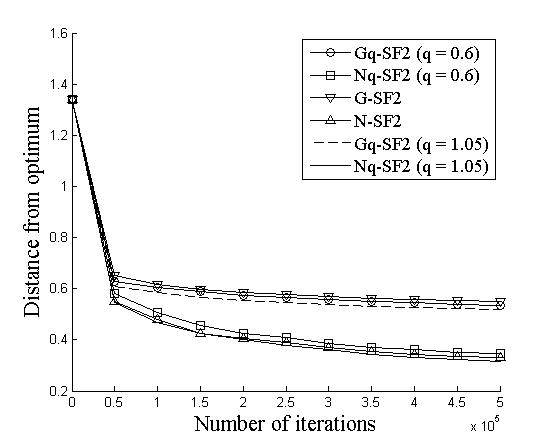
We compare the performance of the Jacobi variant of the N-SF2 algorithm with respect to the corresponding gradient based method (G-SF2) for different values of , and . The other parameters are held fixed at , and . Thus, we perform a total of simulations to obtain parameter updates. The following results are averaged over 20 independent runs, each requiring about 5 seconds of clock time. Fig. 2 shows the convergence behavior of the G-SF2 and N-SF2 for , and Gaussian with and .
Table 1 compares the performance of G-SF2 and N-SF2, for different values of , in terms of the mean and variance of the final distance from the target vector. We note here that, in this case, varies in the range since . The two special cases of Gaussian and Cauchy are retrieved for and , respectively. The table presents a comparison for three values of , viz., and , respectively (comparison for is given in the second and fourth columns of Table 2). The step-size for the Hessian update is fixed with . The results show that although for small (), G-SF2 works better than N-SF2, but for higher , N-SF2 consistently outperforms its gradient counterpart. In fact, it can be observed that the ratio of the distances obtained using G-SF2 and N-SF2 increases with increasing , indicating that the relative performance of N-SF2 in relation to G-SF2 improves with more smoothing. Other observations pertaining to the trends of performance with respect to and are similar to those for G-SF2, discussed in [12].
| N-SF2 | N-SF2 | N-SF2 | G-SF2 | |
|---|---|---|---|---|
| 0.001 | 0.48670.1056 | 0.46980.0627 | 0.43350.0693 | 0.55610.0832 |
| 0.200 | 0.38470.0729 | 0.35890.0591 | 0.36980.0695 | 0.55550.0544 |
| 0.400 | 0.33280.0554 | 0.35470.0548 | 0.39560.0698 | 0.53760.0569 |
| 0.600 | 0.34220.0792 | 0.31630.0582 | 0.32540.0488 | 0.54720.0470 |
| 0.800 | 0.31270.0694 | 0.31360.0699 | 0.33970.0536 | 0.50680.0548 |
| Gaussian | 0.31300.0539 | 0.35600.0488 | 0.33830.0514 | 0.53540.0810 |
| 1.020 | 0.31600.0534 | 0.32230.0397 | 0.37120.0653 | 0.52630.0511 |
| 1.040 | 0.32030.0585 | 0.30810.0552 | 0.33150.0655 | 0.51030.0965 |
| 1.060 | 0.31300.0599 | 0.32160.0566 | 0.36810.0540 | 0.47250.0599 |
| 1.080 | 0.37220.0516 | 0.35840.0633 | 0.37820.0384 | 0.51650.0666 |
| Cauchy | 0.42490.0615 | 0.39970.0509 | 0.44020.0657 | 0.56850.0798 |
| 1.099 | 0.54500.0683 | 0.55940.0623 | 0.56770.0626 | 0.72530.0776 |
We also discuss about the effect of updating the Hessian estimate along different timescales. Table 2 shows the effect of on the N-SF2 algorithm for varying (see earlier discussion), while is held fixed at . It can be observed that, at this level of smoothing, N-SF2 always performs better than G-SF2. For each value of , the best value of is highlighted. A faster update of the Hessian is seen to result in an improved performance. Finally, it is interesting to note from both tables that the best results are most often obtained for values of that do not correspond to either the Gaussian or the Cauchy perturbations, thereby signifying the importance of generalization of the SF algorithms to include -Gaussian perturbations, with a continuously-valued parameter.
6 Conclusions
We proposed a two-simulation SF algorithm with -Gaussian perturbations to perform Newton based optimization of a stochastic objective function. In this process, we derived estimates for the Hessian of a two-sided smoothed functional using -Gaussian distribution. We also derived conditions for convergence of the algorithms, and illustrated the performance of the algorithms through numerical simulations.
An interesting fact here is that though it is known that gradient of -Gaussian SF always converges to the gradient of cost function as smoothing parameter , we observed that the same does not always hold for the Hessian. In particular, we found that the Hessian in the case of uniform () smoothing does not converge. The issue lies in the attempt to derive an expression for the smoothed Hessian, , in terms of the cost function. One can verify that this is not possible for the uniform case since the Hessian of the smoothed functional turns out to be in the form of a finite difference of the gradient of the cost function. Deriving a Hessian estimator for the case of uniform perturbations in terms of objective function remains an open problem.
As suggested in [3], we may vary the smoothing parameter, , at different update iterations. It would be useful to use more smoothing (larger ) at the initial stages to proceed towards the global minimum, whereas at later stages of the algorithm a smaller value of would provide better estimates for the gradient and Hessian. From the analysis point of view, such a modification does not affect the results, where we can easily replace by the corresponding sequence as long as the sequence satisfies the conditions in Assumption IV in place of the sequence . Further, Theorem 7 holds as long as we have .
A similar modification may also be used for the values of . It has been empirically observed, both in Section 5 and in [12], that as decreases, larger values of tend to perform better. Hence, one may start from a high value of and low value of , and can decrease the former and increase the latter as the iterations proceed. One may also incorporate the modification suggested in [30], where steepest descent is employed for the initial parameter updates and Newton based search is employed for faster convergence of later recursions. Such algorithmic modifications can be effectively used to improve the performance of the method and reduce the the computational burden of full Newton methods without affecting the theoretical analysis.
Appendix A Details of convergence analysis
The convergence analysis is based on three key results. The convergence of the gradient and Hessian recursions follow from results in [8] (summarized in Lemma 2). While the main result in our context is given in Lemma 3, Lemma 1 proves a necessary condition required for the application of Lemma 2.
The main theorem for convergence of N-SF2 is based on a result on projected iterated schemes [17]. The conditions in this result require Lemma 5 to hold. While the result in [17] helps to eliminate the effect of the noise term, Proposition 4 shows that the error term is also small and does not affect convergence. A more rigorous way to use the consequences of Proposition 4 would be via Hirsch’s lemma [13]. We provide the intuitive arguments for this in the proof of Theorem 7.
Lastly, most of the proofs given below use a technical result regarding statistical properties of the multivariate -Gaussian distribution [12, Proposition 4.1]. This result provides conditions for existence and an expression for the following expectation
| (42) |
for a standard -dimensional -Gaussian random variate and non-negative integers , , where is as defined in (9). We skip the details of this result, but state few consequences in the following corollary that will be used in later discussions. The claims below immediately follow from [12, Proposition 4.1].
Corollary 8.
The expectation in (42) exists and is finite for when , and the same holds for if . Further, in special cases, we have the following simplifications. Using notations similar to (42), we have
- 1.
the term in (42) is zero whenever at least one of the ’s is odd,
- 2.
,
- 3.
, and
- 4.
for all , . The latter two statements involve a term of , and hence, exist only for , while the first two are defined over the entire range of ’s.
Detailed proofs of results in Section 4
The proofs of Lemmas 1 and 3 and Proposition 4 contain two parts related to the gradient and Hessian. We mostly prove the result for the Hessian case. The corresponding proofs for gradient can be approached in a similar (in fact, simpler) manner, which are presented in [12].
PROOF.
(Proof of Lemma 1)
It is obvious that for all , , which implies is a martingale difference sequence. Using Jensen’s inequality, we have
| (43) |
where we use to denote the 2-norm for the matrices and for . Denoting the Frobenius norm by , we can use the definition of to write
| (44) |
For , we use Holder’s inequality and the fact that to claim
where, from (44), we can argue that is finite for any finite as and for all . Further by the Lipschitz continuity of and Assumption III, we can claim and a.s. Thus, a.s. for all . For , we note the second term in (44) is negative, and hence, we may bound using only the first and third terms as
| (45) |
Applying the Cauchy-Schwartz inequality and the fact that , for any , on the first term in (45), we obtain
The second expectation is finite a.s. from earlier discussion. We expand in the first expectation and use Corollary 8 to claim the existence and finiteness of the expectation for . Similar arguments are applicable for the second term in (45) and the claim follows.
PROOF.
(Proof of Lemma 3)
Since Lemma 1 holds, one can verify that iterations (33) and (34) satisfy the necessary conditions required to apply Lemma 2, where the invariant measure, , of the process is the product measure of and , the invariant measures of the processes and , respectively. The claim follows from an application of the aforementioned result.
PROOF.
(Proof of Proposition 4)
For small , we use Taylor’s expansion of and around to write
Thus the gradient of the two-sided SF (8) becomes
| (46) |
and the two-sided smoothed Hessian (17) is
| (47) |
Let us consider each of the terms in (47). Corollary 8 ensures that the product moments are zero whenever the product is odd. Hence, for all , , . Thus, the off-diagonal terms are zero, whereas the diagonal elements are of the form
| (48) |
for all . Corollary 8 shows that the expectations in (48) exist for . One can note that the squared term in the denominator imposes the condition . Substituting the corresponding expressions in (48), we get . Thus, the first term in (47) is zero. Now, we consider the second term. For ,
which is zero unless or . So using the fact that is symmetric, i.e., , we can write
| (49) |
Referring to Corollary 8, we obtain
for . Now for , we use the definition of (2.2) to write
Since the above expectations are zero for , we have
| (50) |
We again refer to Corollary 8 to compute each term in (50), and then perform simple algebraic manipulations to derive
By substituting all the above expressions in (47), we have that the difference between and is , which implies that the Euclidean distance between and is . A similar result can be shown for the gradient as well.
For the second part of the claim, we write
which implies that
| (51) |
Since is continuously differentiable on the compact set , . Also, since is a positive definite matrix for any matrix , its inverse always exists, i.e., considering any matrix norm. Thus, in order to justify the claim, we need to show that other terms are . From the first part of the claim, we have , and we can write
We note that for any matrix , the eigenvalues of are lower bounded by . Hence, the first two terms, which are upper bounded by the maximum eigenvalues of the inverse of the projected matrices, can at most be . Also we have shown the third term is . The claim follows.
PROOF.
(Proof of Lemma 5)
As is -measurable, while is independent of for all , we can conclude that . Thus is a martingale sequence. Now note as in Lemma 1 that
since the first term in the expectation is square of the maximum eigenvalue of the inverse of the projected Hessian matrix, which can be bounded above by . Using an argument similar to Lemma 1, we can show has bounded variance. Using the fact that , we can write
is finite a.s. From here, the claim follows from the martingale convergence theorem [38, page 111].
PROOF.
(Proof of Theorem 7) Before proving the result, we briefly discuss the roles of Assumptions I–V in the proof. Assumption I is essential for defining the smoothed gradient (8) and Hessian (17), while Assumption II helps us to define the long run cost (19). The existence of the stochastic Lyapunov function (Assumption III) is used for the application of Theorem 2. The assumption on the step-sizes (Assumption IV) is required to ensure the second condition in Theorem 2 and last two conditions of Lemma 6. Here, we note that the square summability of the sequence makes it easy to satisfy the a.s. convergence of the martingale sequence (c.f. Lemma 5). Finally, due to Assumption V, one can prove the claims in Proposition 4 and Lemma 5, and hence, we can apply Kushner and Clark’s result, see [17, Theorem 5.3.1] (alternatively [12, Lemma 4.6]), to claim that the update in (35) converges to the stable fixed points of the ODE
| (52) |
Note that the other condition in Lemma 6 follows from the definition of and , and the continuous differentiability of .
References
- [1] D. P. Bertsekas and J. N. Tsitsiklis. Neuro-dynamic programming. Athena Scientific, Belmont, 1996.
- [2] S. Bhatnagar. Adaptive multivariate three-timescale stochastic approximation algorithms for simulation based optimization. ACM Transactions on Modeling and Computer Simulation (TOMACS), 15(1):74–107, 2005.
- [3] S. Bhatnagar. Adaptive Newton-based multivariate smoothed functional algorithms for simulation optimization. ACM Transactions on Modeling and Computer Simulation, 18(1):27–62, 2007.
- [4] S. Bhatnagar and V. S. Borkar. Two timescale stochastic approximation scheme for simulation-based parametric optimization. Probability in the Engineering and Informational Sciences, 12:519–531, 1998.
- [5] S. Bhatnagar and V. S. Borkar. Multiscale chaotic SPSA and smoothed functional algorithms for simulation optimization. Simulation, 79(9):568–580, 2003.
- [6] S. Bhatnagar, M. C. Fu, S. I. Marcus, and S. Bhatnagar. Two timescale algorithms for simulation optimization of hidden makov models. IIE Transactions, 33(3):245–258, 2001.
- [7] S. Bhatnagar, H. L. Prasad, and L. A. Prasanth. Stochastic Recursive Algorithms for Optimization. Springer, 2013.
- [8] V. S. Borkar. Stochastic Approximation: A Dynamical Systems Viewpoint. Cambridge University Press, 2008.
- [9] D. C. Chin. Comparative study of stochastic algorithms for system optimization based on gradient approximation. IEEE Transactions on Systems, Man and Cybernetics – Part B: Cybernetics, 27(2):244–249, 1997.
- [10] B. Delyon, M. Lavielle, and E. Moulines. Convergence of a stochastic approximation version of the EM algorithm. Annals of Statistics, pages 94–128, 1999.
- [11] D. Ghoshdastidar, A. Dukkipati, and S. Bhatnagar. -Gaussian based smoothed functional algorithms for stochastic optimization. In International Symposium on Information Theory. IEEE, 2012.
- [12] D. Ghoshdastidar, A. Dukkipati, and S. Bhatnagar. On some statistical properties of multivariate -Gaussian distribution. arXiv preprint arXiv:1206.4832v5, 2013.
- [13] M. W. Hirsch. Convergent activation dynamics is in continuous time networks. Neural Networks, 2:331–349, 1989.
- [14] V. Y. A. Katkovnik and Y. U. Kulchitsky. Convergence of a class of random search algorithms. Automation Remote Control, 8:1321–1326, 1972.
- [15] E. Kiefer and J. Wolfowitz. Stochastic estimation of a maximum regression function. Annals of Mathematical Statistics, 23:462–466, 1952.
- [16] J. Kreimer and R. Y. Rubinstein. Nondifferentiable optimization via smooth approximation: General analytical approach. Annals of Operations Research, 39:97–119, 1992.
- [17] H. J. Kushner and D. S. Clark. Stochastic Approximation Methods for Constrained and Unconstrained Systems. Springer-Verlag, New York, 1978.
- [18] H. J. Kushner and H. Huang. Averaging methods for the asymptotic analysis of learning and adaptive systems, with small adjustment rate. SIAM J. Control Optim., 19(5):635–650, 1981.
- [19] L. Ljung. Recursive least-squares and accelerated convergence in stochastic approximation schemes. International Journal of Adaptive Control and Signal Processing, 15(2):169–178, 2001.
- [20] V. Mishra, S. Bhatnagar, and N. Hemachandra. Discrete parameter simulation optimization algorithms with applications to admission control with dependent service times. In Decision and Control, 2007 46th IEEE Conference on, pages 2986–2991, 2007.
- [21] D. Prato and C. Tsallis. Nonextensive foundation of Lévy distributions. Physical Review E., 60(2):2398–2401, 1999.
- [22] M. L. Puterman. Markov decision processes: Discrete stochastic dynamic programming. Wiley, New York, 1994.
- [23] H. Robbins and S. Monro. A stochastic approximation method. Annals of Mathematical Statistics, 22(3):400–407, 1951.
- [24] R. Y. Rubinstein. Simulation and Monte-Carlo Method. John Wiley, New York, 1981.
- [25] D. Ruppert. A Newton-Raphson version of the multivariate Robbins-Monro procedure. Ann. Stat., 13:236–245, 1985.
- [26] P. J. Schweitzer. Perturbation theory and finite Markov chains. J. Appl. Prob., pages 401–413, 1968.
- [27] J. C. Spall. A stochastic approximation technique for generating maximum likelihood parameter estimates. In American Control Conference, 1987, pages 1161–1167, 1987.
- [28] J. C. Spall. Multivariate stochastic approximation using a simultaneous perturbation gradient approximation. IEEE Transactions on Automatic Control, 37(3):332–334, 1992.
- [29] J. C. Spall. A one-measurement form of simultaneous perturbation stochastic approximation. Automatica, 33(1):109–112, 1997.
- [30] J. C. Spall. Adaptive stochastic approximation by the simultaneous perturbation method. IEEE Transactions on Automatic Control, 45:1839–1853, 2000.
- [31] M. A. Styblinski and L. J. Opalski. Algorithms and software tools for ic yield optimization based on fundamental fabrication parameters. Computer-Aided Design of Integrated Circuits and Systems, IEEE Transactions on, 5(1):79–89, 1986.
- [32] M. A. Styblinski and T. S. Tang. Experiments in nonconvex optimization: Stochastic approximation with function smoothing and simulated annealing. Neural Networks, 3(4):467–483, 1990.
- [33] C. Tsallis. Some comments on Boltzmann-Gibbs statistical mechanics. Chaos, Solitons & Fractals, 6:539–559, 1995.
- [34] C. Tsallis, R. S. Mendes, and A. R. Plastino. The role of constraints within generalized nonextensive statistics. Physica A: Statistical Mechanics and its Applications, 261(3–4):534–554, 1998.
- [35] S. Umarov and C. Tsallis. Multivariate generalizations of the -central limit theorem. arXiv:cond-mat/0703533, 2007.
- [36] F. J. Vazquez-Abad and H. J. Kushner. Estimation of the derivative of a stationary measure with respect to a control parameter. J. App. Prob., 29:343–352, 1992.
- [37] C. Vignat and A. Plastino. Central limit theorem and deformed exponentials. Journal of Physics A: Mathematical and Theoretical, 20(45), 2007.
- [38] D. Williams. Probability with Martingales. Cambridge University Press, 1991.
- [39] X. Zhu and J. C. Spall. A modified second-order SPSA optimization algorithm for finite samples. International Journal of Adaptive Control and Signal Process, 16:397–409, 2002.