The one-loop contributions to $\Delta r$ consist of the $W$ boson self-energy, vertex and box diagrams, and the related counter terms (CT),

Here $\Sigma_{T}$ denotes the transverse part of a gauge boson self-energy, $\delta M_{W}$ is the counterterm for the $W$ boson mass, $\delta Z_{e}$ and $\delta s_{\mathrm{w}}$ are the renormalization constants for the electric charge and the (sine of the) weak mixing angle, respectively, while the other $\delta Z$ denote field renormalization constants. Since the $W$ boson appears only as a virtual particle, its field renormalization constant $\delta Z_{W}$ drops out in the $\Delta r$ formula. The box diagrams are themselves UV-finite in a renormalizable gauge. Choosing on-shell renormalization conditions,³³ 3 The on-shell renormalization conditions correspond to the definition of the $W$ and $Z$ boson masses according to the real part of the complex pole of the propagator. This gives rise to the fact that the predictions for $\Delta r$ discussed in this paper internally make use of a definition of the gauge boson masses in terms of a Breit–Wigner shape with a fixed width. The values of the $W$ and $Z$ boson masses according to this fixed-width definition are finally converted into the running-width definition which has been adopted for the determination of the experimental values of $M_{W}$ and $M_{Z}$, see e.g. Ref. [52] for further details. which ensures that Eq. (8) corresponds to the relation between the physical masses of the $W$ and $Z$ bosons, yields (neglecting the masses of the external fermions)⁴⁴ 4 We adopt here the sign conventions for the covariant derivative used in FeynArts [91, 92, 93, 94, 95, 96], which are different for the SM and the MSSM. Accordingly, sgn (the sign of the term involving the SU(2) coupling in the covariant derivative) in Eq. (13) for this choice of convention is $\text{sgn}=-1$ in the SM and $\text{sgn}=+1$ in the MSSM. Eq. (13) agrees with the corresponding formula given in Ref. [17] up to typographical errors in Ref. [17].

with the photon vacuum polarization

Here $\Sigma_{L}$ denotes the left-handed part of a fermion self-energy.

The contributions to $\Delta r$ in the MSSM, besides the ones of SM type, consist of a large number of additional self-energy, vertex and box diagrams containing sfermions, (SUSY) Higgs bosons, charginos and neutralinos in the loop, see also Ref. [17]. In order to determine the contribution to $\Delta r$ from a particular loop diagram, the Born amplitude has to be factored out of the one-loop muon decay amplitude, as shown in Eq. (10). While most loop diagrams directly give a result proportional to the Born amplitude, more complicated spinor structures that do not occur in the SM case arise from box diagrams containing neutralinos and charginos. Those spinor chains can be related to the Born amplitude with the help of Fierz identities and charge conjugation relations. The reduction of the box diagrams to Born-type amplitudes leads to coefficients containing ratios of mass-squared differences of the involved particles. These coefficients can give rise to numerical instabilities in cases of mass degeneracies. In the implementation of our results (which has been carried out in a Mathematica and a Fortran version) special care has been taken of such parameter regions with mass degeneracies or possible threshold effects, so that a numerically stable evaluation is ensured.

At the one-loop level, the quantity $\Delta r$ can be split into three parts

The shift of the fine structure constant $\Delta\alpha$ arises from the charge renormalization which contains the contributions from light fermions. The quantity $\Delta\rho$ contains loop corrections to the $\rho$ parameter [98], which describes the ratio between neutral and charged weak currents, and can be written as

This quantity is sensitive to the mass splitting between the isospin partners in a doublet [98], which leads to a sizable effect in the SM in particular from the heavy fermion doublet. While $\Delta\alpha$ is a pure SM contribution, $\Delta\rho$ can get large contributions also from SUSY particles, in particular the superpartners of the heavy quarks. All other terms, both of SM and SUSY type, are contained in the remainder term $\Delta r_{\text{rem}}$.

The one-loop result described above has been combined with all available higher-order corrections. Since the calculation of $\Delta r$ in the SM is more advanced than in the MSSM we have organized our result such that the full SM result for $\Delta r$ can be used also for the MSSM prediction of $M_{W}$. Therefore the MSSM result is split into a SM part and a SUSY part⁵⁵ 5 Since the complete one-loop results for $\Delta r$ in the SM and in the MSSM are used in Eq. (17), this splitting has an impact only from the two-loop level onwards.

Writing the MSSM result in terms of Eq. (17) ensures in particular that in the decoupling limit of the MSSM result, where all superpartners are heavy and the Higgs sector becomes SM-like, the full SM result (with $M_{H}^{\text{SM}}=M_{h}$) is recovered, see also the discussion in Ref. [17]. The SM part of $\Delta r$ up to four-loop order is given by

It contains, besides the one-loop contribution $\Delta r^{(\alpha)}$,

• •

  the two-loop QCD corrections $\Delta r^{\alpha\alpha_{s}}$ [54, 55, 56, 57, 58, 59],

• •

  the three-loop QCD corrections $\Delta r^{\alpha\alpha_{s}^{2}}$ [65, 66, 67, 68],

• •

  the fermionic electroweak two-loop corrections $\Delta r_{\text{ferm}}^{(\alpha^{2})}$ [60, 52, 61],

• •

  the purely bosonic electroweak two-loop corrections $\Delta r_{\text{bos}}^{(\alpha^{2})}$ [62, 63, 64],

• •

  the mixed QCD and electroweak three-loop contributions $\Delta r^{G_{\mu}^{2}\alpha_{s}m_{t}^{4}}$ [69, 72],

• •

  the purely electroweak three-loop contribution $\Delta r^{G_{\mu}^{3}m_{t}^{6}}$ [69, 72],

• •

  and the four-loop QCD correction $\Delta r^{(G_{\mu}m_{t}^{2}\alpha_{s}^{3})}$ [71].

The full result for the electroweak two-loop contributions in the SM involves numerical integrations of the two-loop scalar integrals, which make the corresponding code rather unwieldy and slow. Thus, we make use of the simple parametrisation that has been given in Ref. [22] for the combined result of the fermionic and bosonic electroweak two-loop corrections in the SM, which approximates the exact result for $\Delta r_{\text{ferm}}^{(\alpha^{2})}+\Delta r_{\text{bos}}^{(\alpha^{2})}$ to better than $2.7\times 10^{-5}$ for $10\,\,\mathrm{GeV}\leq M_{H}^{\text{SM}}\leq 1\,\,\mathrm{TeV}$ (and the other input parameters in their $2\,\sigma$ ranges), corresponding to an uncertainty of $0.4\,\,\mathrm{MeV}$ for $M_{W}$. The use of a parametrisation directly for the SM prediction of $\Delta r_{\text{ferm}}^{(\alpha^{2})}+\Delta r_{\text{bos}}^{(\alpha^{2})}$ rather than for the full SM prediction of $M_{W}$ leads to an improved accuracy in the combination with the SUSY contributions as compared to Ref. [17]. Concerning the QCD corrections, which enter from the two-loop level onwards, it should be noted that they result in a rather large (downward) shift of the $W$ boson mass prediction. It is obvious that this kind of corrections needs to be theoretically well under control in order to gain sensitivity to effects of physics beyond the SM.

The quantity $\Delta r^{\text{SUSY}}$ in Eq. (17) denotes the difference between $\Delta r$ in the MSSM and the SM, i.e. it only involves the contributions from the additional SUSY particles and the extended Higgs sector. Beyond one-loop order, all SUSY corrections that are known to date are implemented, namely the leading reducible ${\cal O}(\alpha^{2})$ two-loop corrections that can be obtained via the resummation formula given in Ref. [99], the leading SUSY two-loop QCD corrections of ${\cal O}(\alpha\alpha_{s})$ to $\Delta\rho$ as given in Refs. [86, 87], as well as the dominant Yukawa-enhanced electroweak corrections of ${\cal O}(\alpha_{t}^{2})$, ${\cal O}(\alpha_{t}\alpha_{b})$, ${\cal O}(\alpha_{b}^{2})$ to $\Delta\rho$ [88, 89]. In order to incorporate the latter corrections, the dominant Yukawa-enhanced electroweak corrections in the SM [100, 101] have been subtracted from the MSSM result presented in Ref. [89] according to Eq. (17). For this purpose we have identified the SM Higgs mass entering the result of Refs. [100, 101] with the mass of the MSSM Higgs boson that has the largest coupling to gauge bosons (i.e., the MSSM Higgs boson that behaves most SM-like). In the decoupling limit, where $M_{A}\gg M_{Z}$ and all superpartners are heavy, the MSSM contribution reduces to the SM contribution with $M_{H}^{\text{SM}}=M_{h}$, so that the contribution to $\Delta r^{\text{SUSY}}$ vanishes as required.

The mass of the signal discovered in the Higgs boson searches at the LHC about a year ago is measured mainly in the $\gamma\gamma$ and the $ZZ^{(*)}$ channels. Currently, the combined mass measurement from ATLAS is $125.5\pm 0.2\pm 0.6{\;\mathrm{GeV}}$ [107] and from CMS $125.7\pm 0.3\pm 0.3{\;\mathrm{GeV}}$ [108]. Adding systematic and statistical errors in quadrature and determining the weighted average between the ATLAS and CMS measurements we get $M_{H}^{\text{SM}}=125.64\pm 0.35\,\,\mathrm{GeV}$. Setting the SM Higgs boson mass to this value, the SM prediction for the $W$ boson mass reads (the other SM parameters have been fixed as $G_{\mu}=1.1663787\times 10^{-5}$, $M_{Z}=91.1875\,\,\mathrm{GeV}$, $\alpha_{s}(M_{Z})=0.1180$, $\Delta\alpha_{\rm had}=0.02757$)

Accordingly, the SM prediction for $M_{W}$ turns out to be below the current experimental value, $M_{W}^{\rm exp}=80.385\pm 0.015\,\,\mathrm{GeV}$, by about $1.5\,\sigma$. The dominant theoretical uncertainty of the prediction for $M_{W}$ arises from the parametric uncertainty induced by the experimental error in the measurement of the top-quark mass. An experimental error of 1 GeV on $m_{t}$ causes a parametric uncertainty on $M_{W}$ of about $6\,\,\mathrm{MeV}$, while the parametric uncertainties induced by the current experimental error of the hadronic contribution to the shift in the fine-structure constant, $\Delta\alpha_{\rm had}$, and by the experimental error of $M_{Z}$ amount to about $2\,\,\mathrm{MeV}$ and $2.5\,\,\mathrm{MeV}$, respectively. The uncertainty of the $M_{W}$ prediction caused by the experimental error of the Higgs mass $\delta M_{H}^{\rm exp}=0.35\,\,\mathrm{GeV}$ is significantly smaller ($\sim 0.2\,\,\mathrm{MeV}$). The uncertainties from unknown higher-order corrections have been estimated to be around $4$ MeV in the SM for a light Higgs boson ($M_{H}^{\text{SM}}<300\,\,\mathrm{GeV}$) [74].

The prediction for $M_{W}$ in the MSSM is affected by additional theoretical uncertainties from unknown higher-order corrections of SUSY type. While in the decoupling limit those additional uncertainties vanish, they can be important if some SUSY particles, in particular in the scalar top and bottom sectors, are relatively light. The combined theoretical uncertainty from unknown higher-order corrections of SM- and SUSY-type has been estimated (for the MSSM with real parameters) in Refs. [89, 17] as $\delta M_{W}=(4.7-9.4)$ MeV, depending on the SUSY mass scale.

In the following we will investigate the prediction for $M_{W}$ in the MSSM based on scans of the MSSM parameters over a wide range (using flat distributions). We have performed two versions of those random scans, one where the top-quark mass is kept fixed at $m_{t}=173.2\,\,\mathrm{GeV}$ and one where also $m_{t}$ is allowed to vary in the scan. Both scans use initially $\sim 5\times 10^{6}$ points, and dedicated smaller scans have been performed in parameter regions where the SUSY contributions to $M_{W}$ are relatively large. The scan ranges are given in Table 1. We have assumed that the value of $M_{1}$ is fixed by the one of $M_{2}$ in terms of the usual GUT relation, $M_{1}=5/3\,s_{\mathrm{w}}^{2}/c_{\mathrm{w}}^{2}\,M_{2}$. As mentioned above, we restrict our numerical analysis to the case of real parameters. We include CKM mixing, but the numerical effect turns out to be negligible (below $0.01\,\,\mathrm{MeV}$ in $M_{W}$). Possible flavor violation in the SUSY sector [19] is neglected here. In order to avoid unphysical parameter regions and regions of numerical instabilities we disregard parameter points for which FeynHiggs indicates a large theoretical uncertainty in the evaluation of the Higgs mass predictions. We furthermore exclude points where stop and sbottom masses are mass-degenerate within less than $0.1\,\,\mathrm{GeV}$ causing numerical instabilities in the gluino corrections of ${\cal O}(\alpha\alpha_{s})$ to $\Delta\rho$.

All MSSM points included in our results have the lightest neutralino as LSP and have SUSY particle masses that pass the lower mass limits from direct searches at LEP. The Higgs and SUSY masses are calculated from the MSSM input parameters using FeynHiggs (version 2.9.4) [103, 104, 105, 106]. In the SM and SUSY higher-order corrections, as listed in Sect. 4.2, the bottom-quark mass has been renormalized in the on-shell scheme. Accordingly, in our evaluation of $M_{W}$ the bottom-quark pole mass, $m_{b}^{\text{pole}}$, is used everywhere. This also applies to the calculation of the sbottom masses from the MSSM input parameters, and we have modified the corresponding routine in FeynHiggs accordingly (in the calculation of the sbottom masses furthermore a $\Delta_{b}$ [109, 110, 111, 112] correction enters, which can be absorbed into an effective bottom-quark mass). For every parameter point we test whether it is allowed by direct Higgs searches using the code HiggsBounds (version 4.0.0) [40, 41, 42]. This code tests the compatibility of the MSSM points with the search limits from LEP, the Tevatron and the LHC. Running HiggsBounds, we take into account the theoretical uncertainties on the Higgs masses using the estimate provided by FeynHiggs.

Our results presented below improve on earlier results given in Ref. [17] in several respects. We study here the impact of both the limits from the Higgs boson searches as well as from the signal observed at about $125.6\,\,\mathrm{GeV}$. Furthermore we investigate constraints from present and possible future limits from searches for SUSY particles. On a more technical level, our analysis incorporates the SUSY two-loop corrections of ${\cal O}(\alpha_{t}^{2})$, ${\cal O}(\alpha_{t}\alpha_{b})$, ${\cal O}(\alpha_{b}^{2})$, which were not included in the scan results presented previously, and we perform a more detailed scan involving a larger number of sampling points.

In this section we study the MSSM prediction for $M_{W}$, starting in Fig. 1 where $M_{W}$ is displayed as a function of the top-quark mass, $m_{t}$, in the SM and the MSSM. The green area shows the MSSM parameter space that is allowed by HiggsBounds and the various other constraints described in the previous subsection. It should be noted that in this plot only the limits from the Higgs searches are considered as constraints on the MSSM parameter space, not the observed signal at about $125.6\,\,\mathrm{GeV}$ (the latter will be discussed below). The region where the MSSM prediction for $M_{W}$ overlaps with the one in the SM is indicated by the red strip, where $M_{H}^{\text{SM}}=125.6\pm 0.7\,\,\mathrm{GeV}$ (corresponding roughly to the $2\,\sigma$ experimental error on $M_{H}$) has been used for the SM prediction. The left plot shows the results on a larger scale, in order to indicate the possible range of the MSSM prediction, while the right plot is a zoom into the parameter region of the MSSM near the experimental central values of $M_{W}$ and $m_{t}$. In order to obtain the MSSM prediction shown as the green band in Fig. 1 we have imposed as an additional restriction a limit on the mass splittings in the stop and sbottom sector, which has been implemented via the conditions $m_{\tilde{t}_{2}}/m_{\tilde{t}_{1}}<2.5$ and $m_{\tilde{b}_{2}}/m_{\tilde{b}_{1}}<2.5$. If no such condition on the mass splittings in the stop and sbottom sector were imposed, even larger values of $M_{W}$ (up to $\sim 80.8\,\,\mathrm{GeV}$) would be possible in the MSSM, see also the discussion in Ref. [17]. Since this parameter region far above the experimental value of $M_{W}$ is of little phenomenological interest, we will not consider it further here. While it is well-known that a non-zero SUSY contribution tends to increase the prediction for $M_{W}$ as compared to the SM case, close inspection of Fig. 1 reveals that there exists a small MSSM (green) region below the overlap region between the MSSM and the SM (red), which is best visible for the largest $m_{t}$ values. The reason for this feature lies in the fact that, as explained above, the SM prediction is shown for the range $M_{H}^{\text{SM}}=125.6\pm 0.7\,\,\mathrm{GeV}$, while no restriction from the signal observed in the Higgs searches has been applied to the MSSM parameter space. As a consequence, the MSSM region (green) contains parameter points where the lightest ${\cal CP}$-even Higgs boson of the MSSM has a mass above the range allowed for $M_{H}^{\text{SM}}$ (and below the upper bound on $M_{h}$ in the MSSM, which increases with increasing $m_{t}$). In the decoupling region, where all superpartners are heavy, the MSSM prediction for $M_{W}$ in this case corresponds to the prediction in the SM with a higher value of $M_{H}^{\text{SM}}$, which yields a lower value of $M_{W}$⁶⁶ 6 It should be noted that a similar kind of feature would occur even if one restricted the predicted value for $M_{h}$ in the MSSM to the same region as the range adopted for $M_{H}^{\text{SM}}$. This is caused by the fact that the additional theoretical uncertainties from unknown higher-order corrections affecting the prediction for $M_{h}$ in the MSSM, which are not present in the SM where $M_{H}^{\text{SM}}$ is a free input parameter, essentially lead to a broadening of the allowed range of $M_{h}$ in the MSSM as compared to $M_{H}^{\text{SM}}$..

The predictions for $M_{W}$ in the SM and the MSSM are compared with the current experimental results for $M_{W}$ and $m_{t}$ [6] which are displayed by the corresponding 68% C.L. ellipse shown in gray. One can see that the SM prediction barely touches the 68% C.L. ellipse, whereas the ellipse is fully contained in the MSSM area. It is obvious that the MSSM contains parameter regions where the MSSM prediction for $M_{W}$ is in very good agreement with the data. On the other hand, also $M_{W}$ values significantly above the experimental value are possible in the MSSM. The latter arise mainly from very light states and a large mass splitting in the stop and sbottom sector (see the discussion below).

Fig. 1 shows that confronting the prediction for $M_{W}$ in the MSSM with the experimental result is of interest both for putting constraints on parameter regions that would give rise to a too high value of $M_{W}$ and for investigating the parameter region where the agreement between the MSSM prediction and the data is in fact better than for the SM case. While the deviation between the SM prediction and the experimental result for $M_{W}$ is statistically not very significant (the SM prediction is well compatible with the experimental result at the 95% C.L.), the pattern that the SM prediction is somewhat low as compared to the data has been robust for many years in spite of numerous updates of the experimental results. Focussing now on the region where we find the best agreement between the MSSM prediction for $M_{W}$ and the experimental result, it is interesting to note that in this region some of the superpartner masses are expected to be relatively light. In order to illustrate this feature we furthermore show in Fig. 1 the impact of the slepton sector (left arrow) and the chargino sector (right arrow), where the mass values indicated at the arrows (approximately) show the effect in $M_{W}$ arising from the contribution of a slepton and a chargino having this mass, respectively. We have chosen to display those arrows such that they start at the lower border, corresponding to the situation where all other superpartners are heavy and decoupled. For the sleptons we show the corrections to $M_{W}$ as a function of $M_{L}\equiv M_{\tilde{E}_{1,2,3}}=M_{\tilde{L}_{1,2,3}}$, where the lower limit of $\sim 90\,\,\mathrm{GeV}$ roughly corresponds to the (fairly model-independent) limit obtained at LEP. One can see that very light sleptons, just above the LEP limit, could induce a shift in $M_{W}$ of about $60\,\,\mathrm{MeV}$. We have checked that each generation contributes roughly the same to this effect. The major contributions to $M_{W}$ from the sleptons arise from the $\Delta\rho$ term in Eq. (15), which is sensitive to the mass splitting between $\tilde{l}_{1,2}$ and $\tilde{\nu_{l}}$. The splitting between the sneutrinos and the sleptons becomes significant if $M_{\tilde{E}}=M_{\tilde{L}}$ and $M_{W}$ are of comparable size. The contributions to $M_{W}$ from light charginos and neutralinos are substantially smaller, but clearly not negligible in this context. They reach about $20\,\,\mathrm{MeV}$ for $m_{\tilde{\chi}^{\pm}_{1}}\sim 95\,\,\mathrm{GeV}$, close to its lower mass limit from LEP. In that case, due to the assumed GUT relation between $M_{1}$ and $M_{2}$, the mass of $\tilde{\chi}^{0}_{1}$ is $\sim 50\,\,\mathrm{GeV}$. Our analysis of the contributions in the slepton and the chargino / neutralino sector shows that even if all squarks were so heavy that their contribution to the $M_{W}$ prediction were negligible, contributions from the slepton sector or the chargino / neutralino sector could nevertheless be sufficient to bring the MSSM prediction in perfect agreement with the data. This could be the case for slepton masses of about $150$–$200\,\,\mathrm{GeV}$ or for a chargino mass of about $100$–$150\,\,\mathrm{GeV}$. If the squark sector gives rise to a non-zero contribution to $M_{W}$ the same predicted value for $M_{W}$ could be reached with heavier sleptons and charginos / neutralinos.

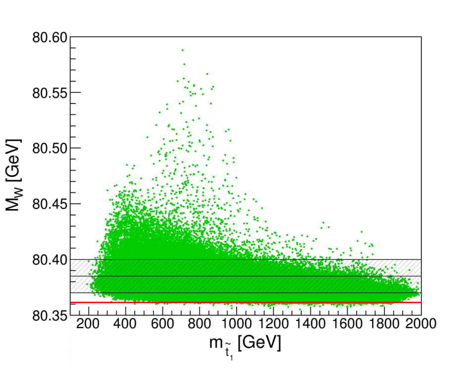
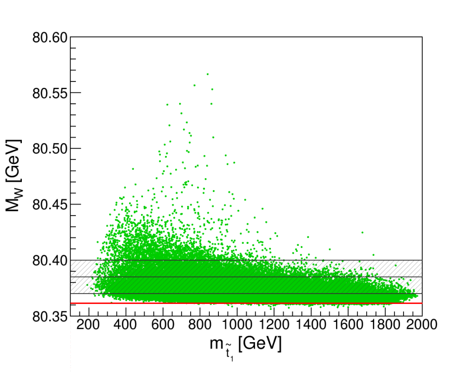
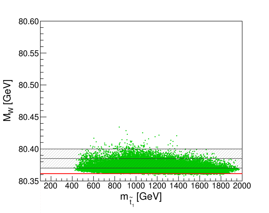
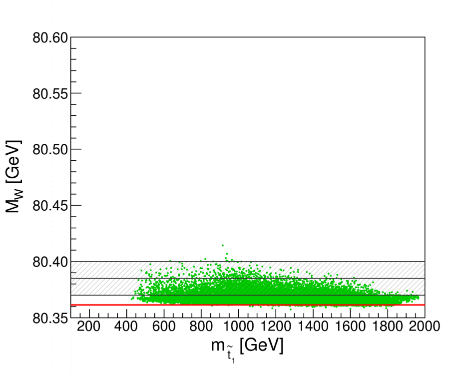
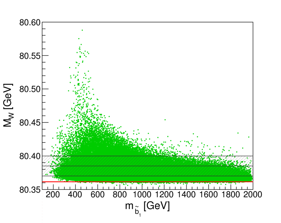
In Fig. 2 and Fig. 3 we analyze in detail the dependence of $M_{W}$ on the scalar quark masses, in particular on $m_{\tilde{t}_{1}}$ and $m_{\tilde{b}_{1}}$, with $m_{t}$ fixed to $173.2\,\,\mathrm{GeV}$. The upper left plot of Fig. 2 shows the prediction for $M_{W}$ (green dots) as a function of $m_{\tilde{t}_{1}}$. All points are allowed by the constraints discussed in Sect. 5.2 and fulfill the additional constraint $m_{\tilde{t}_{2},\tilde{b}_{2}}/m_{\tilde{t}_{1},\tilde{b}_{1}}<2.5$. The SM prediction is shown as a red strip for $M_{H}^{\text{SM}}=125.6\pm 0.7\,\,\mathrm{GeV}$, and the $1\,\sigma$ experimental result is indicated as a gray dashed band. We checked that without the cut $m_{\tilde{t}_{2},\tilde{b}_{2}}/m_{\tilde{t}_{1},\tilde{b}_{1}}<2.5$ the largest $M_{W}$ values are reached for very light stop masses with a very large ($>2.5$) splitting in the stop sector. Now the maximum of $\sim 80.6\,\,\mathrm{GeV}$ is reached for $m_{\tilde{t}_{1}}$ around $800\,\,\mathrm{GeV}$. The position where the maximum is reached depends strongly on the splitting between stops and sbottoms and will be further explained below (in the discussion of Fig. 3). In the upper right plot we only show points which have first and second generation squark masses and the gluino mass above $1.2\,\,\mathrm{TeV}$, i.e. roughly at the limit obtained at the LHC for simplified spectra [25, 26, 27, 28]. It can be observed that the effects on $M_{W}$ of the first and second generation squarks as well as of the gluino are rather mild. Next, in the lower left plot we only show points which in addition have $\tilde{b}$ masses above $1000\,\,\mathrm{GeV}$ (this is a hypothetical cut that is applied for illustration purposes only; it does not reflect the current experimental situation). The fact that all MSSM points in the lower left and lower right plots have stop masses larger than $400\,\,\mathrm{GeV}$ results from the restrictions that we have imposed, constraining the sbottom masses ($>1000\,\,\mathrm{GeV}$) and the maximal splitting in the stop and sbottom sector ($m_{\tilde{t}_{2},\tilde{b}_{2}}/m_{\tilde{t}_{1},\tilde{b}_{1}}<2.5$) at the same time. Clearly the sbottoms have a large impact on the $M_{W}$ prediction. After applying (for illustration) the sbottom mass cut the maximal $M_{W}$ values obtained in the scan are $\sim 80.43\,\,\mathrm{GeV}$, i.e. the SUSY contributions can still be so large in this case that they can yield not only predicted $M_{W}$ values that are in good agreement with the experimental result but also ones that are significantly higher. The SUSY shift in this case is caused by the remaining contribution from the stop–sbottom sector, as well as by the contributions from charginos, neutralinos and sleptons. In order to disentangle these effects, in the lower right plot we also require (again, for illustrative purposes only) the electroweak SUSY particles to be heavy and show only points with slepton and chargino masses above $500\,\,\mathrm{GeV}$. A direct mass limit on neutralinos is not applied. Since we fixed $M_{1}\approx\tfrac{1}{2}M_{2}$, all points have neutralino masses above $\sim 240\,\,\mathrm{GeV}$. In this plot the shift in the $M_{W}$ prediction as compared to the SM case arises solely from the stop–sbottom sector with $m_{\tilde{b}_{1}}>1000\,\,\mathrm{GeV}$ (neglecting the numerically insignificant contributions from the other sectors for large SUSY particle masses). One can observe that $M_{W}$ values up to the upper edge of the experimental $1\,\sigma$ band ($\sim 80.400\,\,\mathrm{GeV}$) can still be reached for $m_{\tilde{t}_{1}}$ values as high as $m_{\tilde{t}_{1}}\sim 1100\,\,\mathrm{GeV}$ in this case. For large stop masses, $m_{\tilde{t}_{1}}\gtrsim 1100\,\,\mathrm{GeV}$, the contributions from the stop--sbottom sector decrease as expected in the decoupling limit.⁷⁷ 7 In all plots in Fig. 2 one can see a small gap between the MSSM points for $m_{\tilde{t}_{1}}>1900\,\,\mathrm{GeV}$ and the SM line. This is an artefact of the chosen scan ranges: in this region the mass-splitting between $\tilde{t}_{1}$ and $\tilde{t}_{2}$ is small, and $m_{h}$ does not reach values up to $\sim 126\,\,\mathrm{GeV}$. The $M_{W}$ value approached in the decoupling limit therefore corresponds to the SM prediction for a lower Higgs mass value.

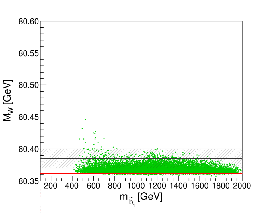
Now we turn to Fig. 3 showing the $M_{W}$ prediction plotted against $m_{\tilde{b}_{1}}$. In the left plot we show all points that are allowed by HiggsBounds and the other constraints described above (in particular, $m_{\tilde{t}_{2}}/m_{\tilde{t}_{1}}<2.5$ and $m_{\tilde{b}_{2}}/m_{\tilde{b}_{1}}<2.5$ is required). In the right plot only those points are displayed for which the stops are heavier than $1000\,\,\mathrm{GeV}$, the first and second generation squark masses as well as the gluino mass are above $1200\,\,\mathrm{GeV}$, and the sleptons and charginos are heavier than $500\,\,\mathrm{GeV}$. Focusing first on the left plot, one can see that it displays the same qualitative features as the upper left plot of Fig. 2. While one would normally expect that the highest values for $M_{W}$ are obtained for the smallest values of $m_{\tilde{t}_{1}}$ and $m_{\tilde{b}_{1}}$, in the corresponding plots of Fig. 2 and Fig. 3 the highest $M_{W}$ values are found for $m_{\tilde{t}_{1}}\sim 800\,\,\mathrm{GeV}$ and $m_{\tilde{b}_{1}}\sim 400\,\,\mathrm{GeV}$. This feature is related to the imposed restriction that the maximal mass splitting for stop and sbottom masses is limited to be smaller than 2.5. The largest correction to $M_{W}$ originates from the stop–sbottom contributions to $\Delta\rho$, which depend sensitively on the mass splittings between the four squarks of the third generation. After imposing the limit on the maximal mass splittings of stops and sbottoms, these contributions become largest if the relative size of the sbottom mixing, $|X_{b}/\mbox{max}(M_{\tilde{Q}_{3}},M_{\tilde{D}_{3}})|$, reaches its maximum. This is realized in this case for $m_{\tilde{b}_{1}}\sim 400\,\,\mathrm{GeV}$ and $m_{\tilde{b}_{2}}/m_{\tilde{b}_{1}}\sim 2.5$, $m_{\tilde{t}_{1}}/m_{\tilde{b}_{1}}\sim 2$, giving rise to the maximum around $m_{\tilde{t}_{1}}\sim 800\,\,\mathrm{GeV}$ and $m_{\tilde{b}_{1}}\sim 400\,\,\mathrm{GeV}$ in the upper left plot of Fig. 2 and the left plot of Fig. 3, respectively. As expected, for higher values of $m_{\tilde{b}_{1}}$ the maximum value reached for $M_{W}$ in Fig. 3 decreases, but $M_{W}$ values as high as the experimental central value are seen to be possible all the way up to $m_{\tilde{b}_{1}}\sim 2\,\,\mathrm{TeV}$. In the right plot the other SUSY particles are required to be rather heavy (in particular, the stop masses are assumed to be above $1000\,\,\mathrm{GeV}$; the other masses are restricted as described above), so that the impact of the contributions from the sbottom sector becomes apparent. While rather large contributions are possible for sbottom masses below about $800\,\,\mathrm{GeV}$, for the highest values of $m_{\tilde{b}_{1}}$ shown in the figure the MSSM prediction for $M_{W}$ approaches the one in the SM.

So far we have only taken into account the existing limits from the Higgs searches at the LHC and other colliders (via the program HiggsBounds), but we have not explicitly imposed a constraint in view of the observed signal at $\sim 125.6\,\,\mathrm{GeV}$. Within the MSSM (referring to the ${\cal CP}$-conserving case for simplicity), the signal can, at least in principle, be identified either with the light ${\cal CP}$-even Higgs boson $h$ or the heavy ${\cal CP}$-even Higgs boson $H$. In Fig. 4 we show the SM and MSSM prediction of $M_{W}$ as a function of $m_{t}$ as obtained from our scan according to Table 1, where in the left plot the green MSSM area fulfills $M_{h}=125.6\pm 3.1\,\,\mathrm{GeV}$, while in the right plot the green MSSM area fulfills $M_{H}=125.6\pm 3.1\,\,\mathrm{GeV}$. The substantially larger uncertainty with respect to the SM experimental uncertainty of $0.7\,\,\mathrm{GeV}$ (at the $2\,\sigma$ level) arises as a consequence of the theoretical uncertainties from unknown higher-order corrections in the MSSM prediction for the Higgs boson mass. We have added a global uncertainty of $3\,\,\mathrm{GeV}$ [104] in quadrature, yielding a total uncertainty of $3.1\,\,\mathrm{GeV}$.

Starting with the left plot, where the light ${\cal CP}$-even Higgs boson has a mass that is compatible with the observed signal, we find a similar result as in Fig. 1. In particular, the comparison with the experimental results for $M_{W}$ and $m_{t}$, indicated by the gray ellipse, shows a slight preference for a non-zero SUSY contribution to $M_{W}$. While the width of the MSSM area shown in green is somewhat reduced compared to Fig. 1 because of the additional constraint applied here (requiring $M_{h}$ to be in the range $M_{h}=125.6\pm 3.1\,\,\mathrm{GeV}$ leads to a constraint on the stop sector parameters, see, e.g., Ref. [32], which in turn limits the maximal contribution to $M_{W}$), the qualitative features are the same as in Fig. 1. This is not surprising, since the limits from the Higgs searches implemented in Fig. 1 have already led to a restriction of the allowed mass range to the unexcluded region near the observed signal. As in Fig. 1 the plot shows a small MSSM region (green) below the overlap region between the MSSM and the SM (red), which is a consequence of the broadening of the allowed range of $M_{h}$ caused by the theoretical uncertainties from unknown higher-order corrections, as explained above.

In the right plot of Fig. 4 we show the result for the case where instead the mass of the heavy ${\cal CP}$-even Higgs boson is assumed to be compatible with the observed signal, i.e. $M_{H}=125.6\pm 3.1\,\,\mathrm{GeV}$. While as mentioned above the interpretation of the discovered signal in terms of the heavy ${\cal CP}$-even Higgs boson within the MSSM is challenged in particular by the recent ATLAS bound on light charged Higgs bosons [39] (which is not yet included in the version of HiggsBounds used for our analysis),⁸⁸ 8 If the Higgs sector contains an additional singlet, as in the NMSSM, it is possible to have a SM-like second-lightest Higgs, while the charged Higgs boson can be much heavier in this case, see e.g. Ref. [113]. it is nevertheless interesting to investigate to what extent the precision observable $M_{W}$ is sensitive to such a rather exotic scenario where all five states of the MSSM Higgs sector are light. The lightest ${\cal CP}$-even Higgs in this scenario has a heavily suppressed coupling to gauge bosons and a mass that can be significantly below the LEP limit for a SM-like Higgs, see e.g. Ref. [33]. As shown in the right plot of Fig. 4, the constraint $M_{H}=125.6\pm 3.1\,\,\mathrm{GeV}$ gives rise to a situation where the MSSM region (green) does not overlap with the SM prediction (blue). This gap between the predictions of the two models is caused by the fact that $M_{H}=125.6\pm 3.1\,\,\mathrm{GeV}$ implies light states in the Higgs sector (in particular a light charged Higgs), which lead to a non-zero SUSY contribution to $M_{W}$ in this case, whereas for the light ${\cal CP}$-even Higgs boson the constraint $M_{h}=125.6\pm 3.1\,\,\mathrm{GeV}$ can be fulfilled in the decoupling region of the MSSM. The plot furthermore shows that the constraint $M_{H}=125.6\pm 3.1\,\,\mathrm{GeV}$ implies not only a lower bound on the SUSY contribution to $M_{W}$ but also a more restrictive upper bound, as can be seen from comparing the two plots in Fig. 4. It is interesting to note that also in the case where the heavy ${\cal CP}$-even Higgs is in the mass range compatible with the observed signal, the MSSM turns out to be better compatible with the experimental results for $M_{W}$ and $m_{t}$ (indicated by the gray ellipse) than the SM.

In Fig. 5 we analyze the dependence of the $M_{W}$ prediction on light scalar taus. In Refs. [114, 115] it was shown that light scalar taus can enhance the decay rate of the light ${\cal CP}$-even Higgs boson into photons. This is of interest in view of the current experimental situation, where the signal strength in the $\gamma\gamma$ channel observed by ATLAS [116] lies significantly above the value expected in the SM (but is still compatible at the $2\,\sigma$ level), while the signal strength observed in CMS [117] is currently slightly below the SM level. Since loop contributions of BSM particles to the decay width $\Gamma(h\to\gamma\gamma)$ do not have to compete with a SM-type tree-level contribution, this loop-induced quantity is of particular relevance for investigating possible deviations from the SM prediction. Fig. 5 shows the prediction for $M_{W}$ as a function of $\Gamma(h\to\gamma\gamma)/\Gamma(H\to\gamma\gamma)_{\mathrm{SM}}$, where the latter has been evaluated with FeynHiggs. As a starting point we use the best-fit point obtained in Ref. [34] from a pMSSM-7 fit to all Higgs data (available at that time), which indeed exhibited an enhancement of $\Gamma(h\to\gamma\gamma)$ due to scalar taus with a mass close to $100\,\,\mathrm{GeV}$. The parameters of the best fit point are $M_{A}=669\,\,\mathrm{GeV}$, $\tan\beta=16.5$, $\mu=2640\,\,\mathrm{GeV}$, $M_{\tilde{Q}_{3}}=M_{\tilde{U}_{3}}=M_{\tilde{D}_{3}}=1100\,\,\mathrm{GeV}$, $M_{\tilde{Q}_{1,2}}=M_{\tilde{U}_{1,2}}=M_{\tilde{D}_{1,2}}=1000\,\,\mathrm{GeV}$, $M_{\tilde{L}_{3}}=M_{\tilde{E}_{3}}=285\,\,\mathrm{GeV}$, $M_{\tilde{L}_{1,2}}=M_{\tilde{E}_{1,2}}=300\,\,\mathrm{GeV}$, $A_{f}=2569\,\,\mathrm{GeV}$, $M_{2}=201\,\,\mathrm{GeV}$ and $M_{3}=1000\,\,\mathrm{GeV}$. In Fig. 5 the best-fit point is indicated as a black star. We vary the stau mass scale $M_{\tilde{E}_{3}}=M_{\tilde{L}_{3}}$ in the range of $280\,\,\mathrm{GeV}$ to $500\,\,\mathrm{GeV}$, giving rise to a corresponding variation of the lighter stau mass. The results are shown as the green line in Fig. 5, where the current experimental $1\,\sigma$ region for $M_{W}$ is indicated as a gray band. One can observe that for light scalar taus, corresponding to larger $\Gamma(h\to\gamma\gamma)$, the agreement of the prediction for $M_{W}$ with the experimental value is improved. A certain level of enhancement of $\Gamma(h\to\gamma\gamma)$ is also compatible with the current experimental results on the signal strength in the $\gamma\gamma$ channel. For heavy scalar taus, as obtained for $M_{\tilde{E}_{3}}=M_{\tilde{L}_{3}}=500\,\,\mathrm{GeV}$ (and keeping the other parameters as defined above), the $M_{W}$ prediction still remains within the experimental $1\,\sigma$ band, while nearly SM values for $\Gamma(h\to\gamma\gamma)$ are reached.

In the final step of our investigation we discuss the precision observable $M_{W}$ in the context of possible future scenarios. We first investigate the impact of an assumed limit of $500\,\,\mathrm{GeV}$ on stops and sbottoms (and assume that no other colored particles are observed below $1200\,\,\mathrm{GeV}$).

In Fig. 6 we show again the $M_{W}$–$m_{t}$ planes as presented in Fig. 1 (where the parameter region allowed by HiggsBounds is displayed) and in Fig. 4 ($M_{h}$ or $M_{H}$ in the range of $125.6\pm 3.1\,\,\mathrm{GeV}$), but now in addition the light blue points obey the (hypothetical) mass limits for stops and sbottoms ($500\,\,\mathrm{GeV}$) and for other colored particles ($1200\,\,\mathrm{GeV}$). The left plot shows the HiggsBounds allowed points, whereas in the middle (right) plot $M_{h}(M_{H})=125.6\pm 3.1\,\,\mathrm{GeV}$ is required. It can be observed that the light blue points corresponding to a relatively heavy colored spectrum are found at the lower end of the predicted $M_{W}$ range, i.e. in the decoupling region of the MSSM. As discussed above the largest SUSY contributions arise from the stop–sbottom sector. If lower lower mass limits on stops and sbottoms of $500\,\,\mathrm{GeV}$ are assumed, it can be seen that the band corresponding to the possible range of predictions for $M_{W}$ in the MSSM would shrink significantly, to the region populated by the blue points. It should be noted that the prediction for $M_{W}$ in this region is in perfect agreement with the experimental measurements of $M_{W}$ and $m_{t}$. Besides the contributions of stops and sbottoms, which can still be significant even if the stops and sbottoms are heavier than $500\,\,\mathrm{GeV}$, the main SUSY corrections arise from relatively light sleptons, charginos and neutralinos, as analyzed above.

While so far we have compared the various predictions with the current experimental results for $M_{W}$ and $m_{t}$, we now discuss the impact of future improvements of these measurements. For the $W$ boson mass we assume an improvement of a factor three compared to the present case down to $\Delta M_{W}=5\,\,\mathrm{MeV}$ from future measurements at the LHC and a prospective Linear Collider (ILC) [118], while for $m_{t}$ we adopt the anticipated ILC accuracy of $\Delta m_{t}=100\,\,\mathrm{MeV}$ [119]. For illustration we show in Fig. 7 again the left plot of Fig. 4, assuming the mass of the light ${\cal CP}$-even Higgs boson $h$ in the region $125.6\pm 3.1\,\,\mathrm{GeV}$, but supplement the gray ellipse indicating the present experimental results for $M_{W}$ and $m_{t}$ with the future projection indicated by the red ellipse (assuming the same experimental central values). While currently the experimental results for $M_{W}$ and $m_{t}$ are compatible with the predictions of both models (with a slight preference for a non-zero SUSY contribution), the anticipated future accuracies indicated by the red ellipse would clearly provide a high sensitivity for discriminating between the models and for constraining the parameter space of BSM scenarios.

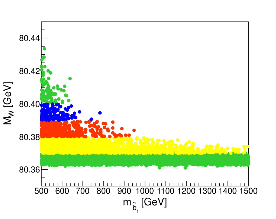
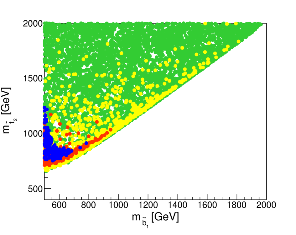
As a further hypothetical future scenario we assume that a light scalar top quark has been discovered at the LHC with a mass of $m_{\tilde{t}_{1}}=400\pm 40\,\,\mathrm{GeV}$, while no other new particle has been observed. As before, for this analysis we use an anticipated experimental precision of $\Delta M_{W}=5\,\,\mathrm{MeV}$ (other uncertainties have been neglected in this analysis). Concerning the masses of the other SUSY particles, we assume lower limits of $300\,\,\mathrm{GeV}$ on both sleptons and charginos, $500\,\,\mathrm{GeV}$ on other scalar quarks of the third generation and of $1200\,\,\mathrm{GeV}$ on the remaining colored particles. We have selected the points from our scan accordingly. Any additional particle observation would impose a further constraint and would thus enhance the sensitivity of the parameter determination. In Fig. 8 we show the parameter points from our scan that are compatible with the above constraints. All points fulfill $M_{h}=125.6\pm 3.1\,\,\mathrm{GeV}$ and $m_{\tilde{t}_{1}}=400\pm 40\,\,\mathrm{GeV}$. Yellow, red and blue points have furthermore a $W$ boson mass of $M_{W}=80.375,80.385,80.395\pm 0.005\,\,\mathrm{GeV}$, respectively, corresponding to three hypothetical future central experimental values for $M_{W}$. The left plot in Fig. 8 shows the $M_{W}$ prediction as a function of the lighter sbottom mass. Assuming that the experimental central value for $M_{W}$ stays at its current value of $80.385\,\,\mathrm{GeV}$ (red points) or goes up by $10\,\,\mathrm{MeV}$ (blue points), the precise measurement of $M_{W}$ would set stringent upper limits of $\sim 800\,\,\mathrm{GeV}$ (blue) or $\sim 1000\,\,\mathrm{GeV}$ (red) on the possible mass range of the lighter sbottom. As expected, this sensitivity degrades if the experimental central value for $M_{W}$ goes down by $10\,\,\mathrm{MeV}$ (yellow points), which would bring it closer to the SM value given in Eq. (19). The right plot shows the results in the $m_{\tilde{b}_{1}}$–$m_{\tilde{t}_{2}}$ plane. It can be observed that sensitive upper bounds on those unknown particle masses could be set⁹⁹ 9 See also Ref. [120] for a recent analysis investigating constraints on the scalar top sector. based on an experimental value of $M_{W}$ of $80.385\pm 0.005\,\,\mathrm{GeV}$ or $80.395\pm 0.005\,\,\mathrm{GeV}$ (i.e. for central values sufficiently different from the SM prediction). In this situation the precise $M_{W}$ measurement could give interesting indications regarding the search for the heavy stop and the light sbottom (or put the interpretation within the MSSM under tension).

We are grateful to A. Freitas, T. Hahn, A. Kotwal, O. Stål, T. Stefaniak and D. Wackeroth for helpful discussions. This work has been supported by the Collaborative Research Center SFB676 of the DFG, “Particles, Strings and the early Universe”. The work of S.H. was supported in part by CICYT (grant FPA 2010–22163-C02-01) and by the Spanish MICINN’s Consolider-Ingenio 2010 Program under grant MultiDark CSD2009-00064.

References

- [1] ATLAS Collaboration, G. Aad et. al. Phys.Lett. B716 (2012) 1–29, [arXiv:1207.7214]
- [2] CMS Collaboration, S. Chatrchyan et. al. Phys.Lett. B716 (2012) 30–61, [arXiv:1207.7235]
- [3] CDF Collaboration, T. Aaltonen et. al. [arXiv:1203.0275]
- [4] DØ Collaboration, V. M. Abazov et. al. [arXiv:1203.0293]
- [5] ALEPH Collaboration, DELPHI Collaboration, L3 Collaboration, OPAL Collaboration, LEP Electroweak Working Group, J. Alcaraz et. al. [hep-ex/0612034]
- [6] Tevatron Electroweak Working Group [arXiv:1204.0042]
- [7] ALEPH Collaboration, DELPHI Collaboration, L3 Collaboration, OPAL Collaboration, SLD Collaboration, LEP Electroweak Working Group, SLD Electroweak Group, SLD Heavy Flavour Group, S. Schael et. al. Phys.Rept. 427 (2006) 257–454, [hep-ex/0509008], see: http://lepewwg.web.cern.ch/LEPEWWG/
- [8] S. Heinemeyer, S. Kraml, W. Porod, and G. Weiglein JHEP 0309 (2003) 075, [hep-ph/0306181]
- [9] S. Heinemeyer and G. Weiglein [arXiv:1007.5232]
- [10] D. Stöckinger J.Phys. G34 (2007) R45–R92, [hep-ph/0609168]
- [11] J. P. Miller, E. d. Rafael, B. L. Roberts, and D. Stöckinger Ann.Rev.Nucl.Part.Sci. 62 (2012) 237–264
- [12] F. Jegerlehner and A. Nyffeler Phys.Rept. 477 (2009) 1–110, [arXiv:0902.3360]
- [13] Heavy Flavor Averaging Group, Y. Amhis et. al. [arXiv:1207.1158], see: http://www.slac.stanford.edu/xorg/hfag
- [14] H. P. Nilles Phys.Rept. 110 (1984) 1–162
- [15] H. E. Haber and G. L. Kane Phys.Rept. 117 (1985) 75–263
- [16] R. Barbieri Riv.Nuovo Cim. 11N4 (1988) 1–45
- [17] S. Heinemeyer, W. Hollik, D. Stöckinger, A. M. Weber, and G. Weiglein JHEP 08 (2006) 052, [hep-ph/0604147]
- [18] S. Heinemeyer, W. Hollik, and G. Weiglein Phys.Rept. 425 (2006) 265–368, [hep-ph/0412214]
- [19] S. Heinemeyer, W. Hollik, F. Merz, and S. Penaranda Eur.Phys.J. C37 (2004) 481–493, [hep-ph/0403228]
- [20] O. Stål, G. Weiglein, and L. Zeune, in preparation
- [21] F. Domingo and T. Lenz JHEP 1107 (2011) 101, [arXiv:1101.4758]
- [22] M. Awramik, M. Czakon, and A. Freitas JHEP 11 (2006) 048, [hep-ph/0608099]
- [23] P. Z. Skands and D. Wicke Eur.Phys.J. C52 (2007) 133–140, [hep-ph/0703081]
- [24] A. H. Hoang and I. W. Stewart Nucl.Phys.Proc.Suppl. 185 (2008) 220–226, [arXiv:0808.0222]
- [25] J. Boyd, talk given at SUSY2013, see: http://susy2013.ictp.it/lecturenotes/03_Wednesday/Boyd.pdf
- [26] J. Richman, talk given at SUSY2013, see: http://susy2013.ictp.it/lecturenotes/03_Wednesday/Richman.pdf
- [27] ATLAS Collaboration, see: https://twiki.cern.ch/twiki/bin/view/AtlasPublic/SupersymmetryPublicResults
- [28] CMS Collaboration, see: https://twiki.cern.ch/twiki/bin/view/CMSPublic/PhysicsResultsSUS
- [29] T. J. LeCompte and S. P. Martin Phys.Rev. D84 (2011) 015004, [arXiv:1105.4304]
- [30] R. Mahbubani, M. Papucci, G. Perez, J. T. Ruderman, and A. Weiler [arXiv:1212.3328]
- [31] Particle Data Group, J. Beringer et. al. Phys.Rev. D86 (2012) 010001, and 2013 partial update for the 2014 edition
- [32] S. Heinemeyer, O. Stål, and G. Weiglein Phys.Lett. B710 (2012) 201–206, [arXiv:1112.3026]
- [33] M. Carena, S. Heinemeyer, O. Stål, C. Wagner, and G. Weiglein Eur. Phys. J. C73 (2013) 2552, [arXiv:1302.7033]
- [34] P. Bechtle, S. Heinemeyer, O. Stal, T. Stefaniak, G. Weiglein, et. al. Eur.Phys.J. C73 (2013) 2354, [arXiv:1211.1955]
- [35] A. Bottino, N. Fornengo, and S. Scopel Phys.Rev. D85 (2012) 095013, [arXiv:1112.5666]
- [36] M. Drees Phys.Rev. D86 (2012) 115018, [arXiv:1210.6507]
- [37] K. Hagiwara, J. S. Lee, and J. Nakamura JHEP 1210 (2012) 002, [arXiv:1207.0802]
- [38] A. Arbey, M. Battaglia, A. Djouadi, and F. Mahmoudi JHEP 1209 (2012) 107, [arXiv:1207.1348]
- [39] ATLAS Collaboration, ATLAS-CONF-2013-090
- [40] P. Bechtle, O. Brein, S. Heinemeyer, O. Stål, T. Stefaniak, et. al. [arXiv:1301.2345]
- [41] P. Bechtle, O. Brein, S. Heinemeyer, G. Weiglein, and K. E. Williams Comput.Phys.Commun. 182 (2011) 2605–2631, [arXiv:1102.1898]
- [42] P. Bechtle, O. Brein, S. Heinemeyer, G. Weiglein, and K. E. Williams Comput.Phys.Commun. 181 (2010) 138–167, [arXiv:0811.4169]
- [43] P. Bechtle, O. Brein, S. Heinemeyer, O. Stål, T. Stefaniak, et. al. [arXiv:1311.0055]
- [44] M. Arana-Catania, S. Heinemeyer, M. Herrero, and S. Penaranda JHEP 1205 (2012) 015, [arXiv:1109.6232]
- [45] MuLan Collaboration, D. Webber et. al. Phys.Rev.Lett. 106 (2011) 041803, [arXiv:1010.0991]
- [46] R. Behrends, R. Finkelstein, and A. Sirlin Phys.Rev. 101 (1956) 866–873
- [47] T. Kinoshita and A. Sirlin Phys.Rev. 113 (1959) 1652–1660
- [48] T. van Ritbergen and R. G. Stuart Nucl.Phys. B564 (2000) 343–390, [hep-ph/9904240]
- [49] M. Steinhauser and T. Seidensticker Phys.Lett. B467 (1999) 271–278, [hep-ph/9909436]
- [50] A. Pak and A. Czarnecki Phys.Rev.Lett. 100 (2008) 241807, [arXiv:0803.0960]
- [51] A. Sirlin Phys.Rev. D22 (1980) 971–981
- [52] A. Freitas, W. Hollik, W. Walter, and G. Weiglein Nucl.Phys. B632 (2002) 189–218, [hep-ph/0202131], [Erratum-ibid. B666 (2003) 305-307]
- [53] W. Marciano and A. Sirlin Phys.Rev. D22 (1980) 2695
- [54] A. Djouadi and C. Verzegnassi Phys. Lett. B195 (1987) 265
- [55] A. Djouadi Nuovo Cim. A100 (1988) 357
- [56] B. Kniehl Nucl. Phys. B347 (1990) 86
- [57] F. Halzen and B. Kniehl Nucl. Phys. B353 (1991) 567
- [58] B. Kniehl and A. Sirlin Nucl. Phys. B371 (1992) 141
- [59] B. Kniehl and A. Sirlin Phys. Rev. D47 (1993) 883
- [60] A. Freitas, W. Hollik, W. Walter, and G. Weiglein Phys.Lett. B495 (2000) 338–346, [hep-ph/0007091], [Erratum-ibid. B570 (2003) 260-264]
- [61] M. Awramik and M. Czakon Phys. Lett. B568 (2003) 48, [hep-ph/0305248]
- [62] M. Awramik and M. Czakon Phys. Rev. Lett. 89 (2002) 241801, [hep-ph/0208113]
- [63] A. Onishchenko and O. Veretin Phys. Lett. B551 (2003) 111, [hep-ph/0209010]
- [64] M. Awramik, M. Czakon, A. Onishchenko, and O. Veretin Phys. Rev. D68 (2003) 053004, [hep-ph/0209084]
- [65] L. Avdeev, J. Fleischer, S. Mikhailov, and O. Tarasov Phys.Lett. B336 (1994) 560, [hep-ph/9406363]
- [66] K. G. Chetyrkin, J. H. Kühn, and M. Steinhauser Phys. Lett. B351 (1995) 331, [hep-ph/9502291]
- [67] K. G. Chetyrkin, J. Kühn, and M. Steinhauser Phys. Rev. Lett. 75 (1995) 3394, [hep-ph/9504413]
- [68] K. Chetyrkin, J. Kühn, and M. Steinhauser Nucl.Phys. B482 (1996) 213, [hep-ph/9606230]
- [69] M. Faisst, J. H. Kühn, T. Seidensticker, and O. Veretin Nucl. Phys. B665 (2003) 649, [hep-ph/0302275]
- [70] K. Chetyrkin, M. Faisst, J. H. Kühn, P. Maierhofer, and C. Sturm Phys.Rev.Lett. 97 (2006) 102003, [hep-ph/0605201]
- [71] R. Boughezal and M. Czakon Nucl.Phys. B755 (2006) 221, [hep-ph/0606232]
- [72] J. van der Bij, K. Chetyrkin, M. Faisst, G. Jikia, and T. Seidensticker Phys.Lett. B498 (2001) 156–162, [hep-ph/0011373]
- [73] R. Boughezal, J. Tausk, and J. van der Bij Nucl.Phys. B713 (2005) 278–290, [hep-ph/0410216]
- [74] M. Awramik, M. Czakon, A. Freitas, and G. Weiglein Phys.Rev. D69 (2004) 053006, [hep-ph/0311148]
- [75] R. Barbieri and L. Maiani Nucl.Phys. B224 (1983) 32
- [76] C. Lim, T. Inami, and N. Sakai Phys.Rev. D29 (1984) 1488
- [77] E. Eliasson Phys.Lett. B147 (1984) 65
- [78] Z. Hioki Prog.Theor.Phys. 73 (1985) 1283
- [79] J. Grifols and J. Sola Nucl.Phys. B253 (1985) 47
- [80] R. Barbieri, M. Frigeni, F. Giuliani, and H. Haber Nucl.Phys. B341 (1990) 309–321
- [81] M. Drees and K. Hagiwara Phys.Rev. D42 (1990) 1709–1725
- [82] M. Drees, K. Hagiwara, and A. Yamada Phys.Rev. D45 (1992) 1725–1743
- [83] P. H. Chankowski, A. Dabelstein, W. Hollik, W. Mosle, S. Pokorski, and J. Rosiek Nucl.Phys. B417 (1994) 101
- [84] D. Garcia and J. Sola Mod.Phys.Lett. A9 (1994) 211–224
- [85] D. M. Pierce, J. A. Bagger, K. T. Matchev, and R.-j. Zhang Nucl.Phys. B491 (1997) 3–67, [hep-ph/9606211]
- [86] A. Djouadi, P. Gambino, S. Heinemeyer, W. Hollik, C. Junger, and G. Weiglein Phys.Rev.Lett. 78 (1997) 3626, [hep-ph/9612363]
- [87] A. Djouadi, P. Gambino, S. Heinemeyer, W. Hollik, C. Junger, and G. Weiglein Phys.Rev. D57 (1998) 4179, [hep-ph/9710438]
- [88] S. Heinemeyer and G. Weiglein JHEP 0210 (2002) 072, [hep-ph/0209305]
- [89] J. Haestier, S. Heinemeyer, D. Stöckinger, and G. Weiglein JHEP 0512 (2005) 027, [hep-ph/0508139]
- [90] Wolfram Research, Inc., Mathematica, Version 8.0, Champaign, IL (2010)
- [91] J. Küblbeck, M. Böhm, and A. Denner Comput.Phys.Commun. 60 (1990) 165–180
- [92] A. Denner, H. Eck, O. Hahn, and J. Küblbeck Phys.Lett. B291 (1992) 278–280
- [93] A. Denner, H. Eck, O. Hahn, and J. Küblbeck Nucl.Phys. B387 (1992) 467–484
- [94] J. Küblbeck, H. Eck, and R. Mertig Nucl.Phys.Proc.Suppl. 29A (1992) 204–208
- [95] T. Hahn Comput.Phys.Commun. 140 (2001) 418, [hep-ph/0012260]
- [96] T. Hahn and C. Schappacher Comput.Phys.Commun. 143 (2002) 54–68, [hep-ph/0105349]
- [97] T. Hahn and M. Perez-Victoria Comput.Phys.Commun. 118 (1999) 153, [hep-ph/9807565]
- [98] M. Veltman Nucl.Phys. B123 (1977) 89
- [99] M. Consoli, W. Hollik, and F. Jegerlehner Phys.Lett. B227 (1989) 167
- [100] R. Barbieri, M. Beccaria, P. Ciafaloni, G. Curci, and A. Vicere Nucl.Phys. B409 (1993) 105–127
- [101] J. Fleischer, O. Tarasov, and F. Jegerlehner Phys.Lett. B319 (1993) 249–256
- [102] T. Hahn, S. Heinemeyer, W. Hollik, H. Rzehak, and G. Weiglein Comput.Phys.Commun. 180 (2009) 1426–1427
- [103] M. Frank, T. Hahn, S. Heinemeyer, W. Hollik, H. Rzehak, et. al. JHEP 0702 (2007) 047, [hep-ph/0611326]
- [104] G. Degrassi, S. Heinemeyer, W. Hollik, P. Slavich, and G. Weiglein Eur.Phys.J. C28 (2003) 133–143, [hep-ph/0212020]
- [105] S. Heinemeyer, W. Hollik, and G. Weiglein Eur.Phys.J. C9 (1999) 343–366, [hep-ph/9812472]
- [106] S. Heinemeyer, W. Hollik, and G. Weiglein Comput.Phys.Commun. 124 (2000) 76–89, [hep-ph/9812320]
- [107] ATLAS Collaboration ATLAS-CONF-2013-014, ATLAS-COM-CONF-2013-025
- [108] CMS Collaboration CMS-PAS-HIG-13-005
- [109] R. Hempfling Phys.Rev. D49 (1994) 6168–6172
- [110] L. J. Hall, R. Rattazzi, and U. Sarid Phys.Rev. D50 (1994) 7048–7065, [hep-ph/9306309]
- [111] M. S. Carena, M. Olechowski, S. Pokorski, and C. Wagner Nucl.Phys. B426 (1994) 269–300, [hep-ph/9402253]
- [112] M. S. Carena, D. Garcia, U. Nierste, and C. E. Wagner Nucl.Phys. B577 (2000) 88–120, [hep-ph/9912516]
- [113] O. Stål and G. Weiglein JHEP 1201 (2012) 071, [arXiv:1108.0595]
- [114] M. Carena, S. Gori, N. R. Shah, C. E. Wagner, and L.-T. Wang JHEP 1207 (2012) 175, [arXiv:1205.5842]
- [115] M. Carena, S. Gori, N. R. Shah, and C. E. Wagner JHEP 1203 (2012) 014, [arXiv:1112.3336]
- [116] ATLAS Collaboration ATLAS-CONF-2013-012
- [117] CMS Collaboration CMS-PAS-HIG-13-001
- [118] M. Baak, A. Blondel, A. Bodek, R. Caputo, T. Corbett, et. al. [arXiv:1310.6708]
- [119] H. Baer, T. Barklow, K. Fujii, Y. Gao, A. Hoang, et. al. [arXiv:1306.6352]
- [120] V. Barger, P. Huang, M. Ishida, and W.-Y. Keung Phys.Lett. B718 (2013) 1024–1030, [arXiv:1206.1777]