跳到论文正文
W Papers独立论文阅读器 arXiv:1311.1545 论文正文 计算阅读时间 · 0%
引用这篇论文根据当前论文元数据生成,正式投稿前建议核对。


License: arXiv.org perpetual non-exclusive license
arXiv:1311.1545v3 [q-fin.PR] 14 Jun 2016

Varadhan’s formula, conditioned diffusions, and local volatilities Thanks:  Corresponding author: Stefano De Marco, Ecole Polytechnique-CMAP, Route de Saclay, 91128 Palaiseau Cedex, France. demarco@cmap.polytechnique.fr
Key words and phrases: conditional density asymptotics, local volatility, stochastic volatility, large deviations.
2010 Mathematics Subject Classification: AMS 91G20, 91G80, 60H30, 65C30.

Stefano De Marco    Peter Friz Affiliation: Ecole Polytechnique, TU and WIAS Berlin
Abstract

Motivated by marginals-mimicking results for Itô processes [14, 24] via SDEs and by their applications to volatility modeling in finance, we discuss the weak convergence of the law of a hypoelliptic diffusions conditioned to belong to a target affine subspace at final time, namely ℒ⁡(Zt|Yt=y)\mathcal{L}(Z_{t}|Y_{t}=y) if X⋅=(Y⋅,Z⋅)X_{\cdot}=(Y_{\cdot},Z_{\cdot}). To do so, we revisit Varadhan-type estimates in a small-noise (as opposed to small-time) regime, studying the density of the lower-dimensional component YY. The application to stochastic volatility models include the small-time and, for certain models, the large-strike asymptotics of the Gyöngy–Dupire local volatility function. The final product are asymptotic formulae that can (i) motivate parameterizations of the local volatility surface and (ii) be used to extrapolate local volatilities in a given model.

1 Introduction

Consider an nn-dimensional diffusion process given by the solution of

d​Xt=b⁡(Xt)​d​t+∑j=1dσj​(Xt)​d​Wtj,X0=x0∈ℝn.dX_{t}=b\left(X_{t}\right)dt+\sum_{j=1}^{d}\sigma_{j}\left(X_{t}\right)dW^{j}_{t},\ X_{0}=x_{0}\in\mathbb{R}^{n}. (1.1)

Applications to finance suggest a splitting of the state space, say X=(Y,Z)∈ℝl×ℝn−l≅ℝnX=(Y,Z)\in\mathbb{R}^{l}\times\mathbb{R}^{n-l}\cong\mathbb{R}^{n}, where YY is the main process of interest (for instance: price or log-price of an asset) and ZZ some auxiliary process (for instance: stochastic volatility, possibly multi-dimensional). There is a massive amount of literature concerning ptp_{t}, the probability distribution function of XtX_{t} at small times tt. In the elliptic case, that is when s​p​a​n​{σ1,…,σd}=ℝnspan\{\sigma_{1},...,\sigma_{d}\}=\mathbb{R}^{n} such investigations go back to Varadhan (“2​t​log⁡pt​(x,y)∼d2​(x,y)2t\log p_{t}(x,y)\sim d^{2}(x,y)”) and then Molchanov [37] for full expansions of ptp_{t}. The hypoelliptic situation (assuming the strong Hörmander condition L​i​e​{σ1,…,σd}=ℝnLie\{\sigma_{1},...,\sigma_{d}\}=\mathbb{R}^{n}) was then studied by Azencott, Bismut, Leandre, Ben Arous,… (the function dd is then be interpreted as control distance associated to the diffusion vector fields.)

Similar results were recently obtained for ftf_{t}, the density of YtY_{t} (that is, a marginal density of XtX_{t}) by Deuschel et al. see [12, 13], improving on earlier works of Takanobu–Watanabe [41]. We postpone a detailed comparison of [41] and our results to Section 1.2 below.

Our main results are: (i) a Varadhan formula for ftf_{t} in the short time limit, which is seen to be valid in great generality (without the need to check for the non-degeneracy conditions that appear as assumptions in [41, 12, 13]11 1 As was seen in [13], checking non-focality requires a non–trivial analysis of certain Hamiltonian systems. We also note that focality actually happens in reasonably simple situations, e.g. in the context of a 2-dimensional Black–Scholes basket, as was seen in [15].) and then (ii) a limit theorem for ZZ conditioned on the value of YY. As far as we know, even in the elliptic case our results, concerning the marginals of XtX_{t}, are new. The limit here may again be short time or, more generally, small noise. In fact, the small noise situations poses new difficulties (for instance, in a strictly hypoelliptic setting Varadhan’s formula may fail!) but then offers new applications: indeed, contribution (iii) of this paper is concerned with a class of stochastic volatility models introduced by Stein–Stein: we exploit scaling in a way that the small noise asymptotics for the conditioned diffusions gives us a (computable) expression for the asymptotic slope of local variance (the square of Dupire’s local volatility as induced from option prices). Postponing precise assumptions to Section 2, our first main result is stated as follows

Theorem 1.1.

(i) Let Xt=(Yt,Zt)X_{t}=(Y_{t},Z_{t}) as above. Under a strong Hörmander condition, YtY_{t} admits a density ftf_{t} for t>0t>0 and the following Varadhan type formula holds: for every y∈ℝly\in\mathbb{R}^{l}

limt→0tlogft(y)=−inf{x=(y,z):z∈ℝn−l}Λ(x)=:Λ(Ny)\lim_{t\to 0}t\log f_{t}(y)=-\inf_{\{x=(y,z):z\in\mathbb{R}^{n-l}\}}\Lambda(x)=:\Lambda(N_{y})

where 2​Λ​(x)=d2​(x0,x)2\Lambda(x)=d^{2}(x_{0},x) is the squared control distance associated to {σ1,…,σd}\{\sigma_{1},...,\sigma_{d}\} and Ny={xN_{y}=\{x =(y,z):z∈ℝn−l}=(y,z):z\in\mathbb{R}^{n-l}\}.

(ii) Under a further technical assumption (always satisfied in the elliptic case - see Thm 2.10 for a precise statement)

ℒ⁡(Zt|Yt=y)⟹δz∗​(y)as ​t↓0\mathcal{L}\left(Z_{t}|Y_{t}=y\right)\Longrightarrow\delta_{z^{\ast}(y)}\qquad\text{as }t\downarrow 0 (1.2)

in the sense of weak convergence of probability measures, provided there exists a unique minimizer z∗​(y)z^{\ast}(y) for the problem argminx∈Ny​Λ​(x)\mbox{argmin}_{x\in N_{y}}\Lambda(x).

While the above theorem is clearly useful (it implies, for instance, short time asymptotics for local volatility; on a technical level, we remove the ellipticity requirement from [7]), it does not lend itself to understand spatial asymptotics. To this end, we generalize the setup and discuss small noise problems of the form

d​Xtε=bε​(Xtε)​d​t+ε​∑j=1dσj​(Xtε)​d​Wtj,X0ε=x0ε,dX^{\varepsilon}_{t}=b_{\varepsilon}\left(X^{\varepsilon}_{t}\right)dt+\varepsilon\sum_{j=1}^{d}\sigma_{j}\left(X^{\varepsilon}_{t}\right)dW^{j}_{t},\ X_{0}^{\varepsilon}=x_{0}^{\varepsilon}, (1.3)

with x0ε→x0x_{0}^{\varepsilon}\to x_{0} and bε→b0b_{\varepsilon}\rightarrow b_{0} (in the precise sense of condition (1.13) below). By Brownian scaling, the short time setting t→0t\to 0 falls into this setting by taking t=ε2t=\varepsilon^{2}, bε=ε2​bb_{\varepsilon}=\varepsilon^{2}b and x0ε=x0x_{0}^{\varepsilon}=x_{0}.

Theorem 1.2.

(i) Write Xtε=(Ytε,Ztε)X^{\varepsilon}_{t}=\left(Y^{\varepsilon}_{t},Z^{\varepsilon}_{t}\right). Under a strong Hörmander condition, and a further technical assumption (which is always satisfied in the elliptic case, or also when b0≡0b_{0}\equiv 0 - see Thm 3.1 for precise assumptions), the following Varadhan type formula holds for the density ftεf^{\varepsilon}_{t} of YtεY^{\varepsilon}_{t}: for every t>0t>0 and y∈ℝly\in\mathbb{R}^{l}

limϵ→0ε2​log⁡ftϵ​(y)=−Λt​(Ny).\lim_{\epsilon\to 0}\varepsilon^{2}\log f^{\epsilon}_{t}(y)=-\Lambda_{t}(N_{y}).

where, as before Ny={x=(y,z):z∈ℝn−l}N_{y}={\{x=(y,z):z\in\mathbb{R}^{n-l}\}}. (Although the action Λ\Lambda is still given in terms of a variational problem, cf. (1.10) below, it has no more the interpretation as point-to-subspace distance.)

(ii) Under the same assumptions as above we have, for fixed yy and t>0t>0,

ℒ⁡(Ztε|Ytε=y)⟹δzt∗​(y)as ​ε↓0\mathcal{L}\left(Z_{t}^{\varepsilon}|Y_{t}^{\varepsilon}=y\right)\Longrightarrow\delta_{z_{t}^{\ast}(y)}\qquad\text{as }\varepsilon\downarrow 0 (1.4)

provided there exists a unique minimizer zt∗​(y)z_{t}^{\ast}(y) for the problem argminx∈Ny​Λt​(x)\mbox{argmin}_{x\in N_{y}}\Lambda_{t}(x).

The case l=nl=n in Theorem 1.1(ii) (“from x0∈ℝnx_{0}\in\mathbb{R}^{n} to x∈ℝnx\in\mathbb{R}^{n}”) is covered by the result of Molchanov [37] for elliptic diffusions, and more recently by Bailleul [2] in the hypoelliptic setting. Besides the more general framework of small noise asymptotics that we consider in Theorem 1.2, in (ii) the final target set for the process XX is an affine subspace instead of a single point (“from x0x_{0} to NyN_{y}”, restoring the point-to-point situation when l=nl=n). Also, the results of [37, 2] are given on compact manifolds, while we work here with ℝn\mathbb{R}^{n}-valued processes, and need to rely on some non-trivial tail bounds.

Following the well-known projection results [24, 14] for Itô SDEs, we then have the following corollaries of Theorem 1.2 for the local volatility:

Theorem 1.3.

(i) [Local volatility, short time behavior] In a generic stochastic volatility model (Y,Z)(Y,Z) (where YY denotes log-price and ZZ stochastic volatility)

σl​o​c2​(t,y)=𝔼⁡[(Zt)2|Yt=y]→z∗​(y)2as ​t→0.\sigma^{2}_{loc}(t,y)=\mathbb{E}[\left(Z_{t}\right)^{2}|Y_{t}=y]\to z^{*}(y)^{2}\qquad\mbox{as }t\to 0. (1.5)

Here z∗=z∗​(y)z^{*}=z^{*}(y) is the “most likely” arrival point, computed as a​r​g​m​i​nargmin of z∈ℝ↦ΛS​V​(y,z)z\in\mathbb{R}\mapsto\Lambda^{SV}(y,z) where ΛS​V​(⋅)\Lambda^{SV}(\cdot) is the action associated to the stochastic volatility model. (Eventually, explicit computations depend on the specific model considered.)

(ii) [Local volatility ‘wings’ in the Stein–Stein model] In the Stein–Stein model (where ZZ follows an Ornstein–Uhlenbeck process, see equation (4.15)) 22 2 When the correlation parameter between the log-price YY and the instantaneous volatility ZZ is not null, the Stein–Stein model is also known as Schöbel and Zhu model, see [39]., small noise asymptotics lead to

limy→±∞σloc2​(t,y)|y|=limy→±∞1|y|​𝔼​[(Zt)2|Yt=y]=ct±>0\lim_{y\to\pm\infty}\frac{\sigma^{2}_{\mathrm{loc}}(t,y)}{|y|}=\lim_{y\to\pm\infty}\frac{1}{|y|}\mathbb{E}[\left(Z_{t}\right)^{2}|Y_{t}=y]=c_{t}^{\pm}>0 (1.6)

where the constants ct±c_{t}^{\pm} are given explicitly in terms of the model parameters.

As we will show in Section 4, under some special parameter configuration of the Stein–Stein model, the explicit expression of the constants ct±c_{t}^{\pm} appearing in (1.6) turns out to be consistent with known results from moment explosion for affine models [30].

As a particular consequence of Theorem 1.3(i), we see that the local volatility surface generated by a fairly general stochastic volatility model (see Theorem 4.4 below for detailed assumptions) does not explode in small time. Conversely, realistic local volatility surfaces typically do exhibit an explosive behavior out of the money when time goes to zero (namely σloc​(t,y)→∞\sigma_{\mathrm{loc}}(t,y)\to\infty as t→0t\to 0, for all y≠0y\neq 0). This is the case for the parametric local volatility surface calibrated to SPX option data in [21, Section 4], and for the local volatilities obtained via Dupire’s formula from realistic SSVI parameterisations [20] of the implied volatility (and finally, the same behavior also appears when applying Dupire’s formula to option prices generated by models with jumps - see a related discussion in [17]). Apart from providing a tool for computing the limit, Theorem 1.3(i) tells precisely that the local volatilities generated by a standard homogeneous stoch vol model based on Brownian diffusions are not able to capture this phenomenon – thus providing a negative result for this class of models, in the same spirit as [18, Theorem 2], which focuses on the behavior of the at-the-money implied volatility skew.

On the other side, in analogy with the large-strike behavior of implied volatility [36, 22], the linear asymptotic behavior of the local variance in Theorem 1.3(ii) is likely to hold in even wider classes of stochastic volatility models (the same result is indeed known to hold for the Heston model, see [11], based on affine principles). On the one hand, the knowledge of an explicit spatial asymptotics for the local volatility can motivate the choice of functional forms used to smooth out and/or extrapolate a local volatility surface calibrated to market data. Already in use among practitioners, SVI-type parameterizations of the local variance, cf. again [21, Section 4], are compatible with the asymptotic result in (1.6). On the other hand, a robust implementation of the local volatility surface isof course the basis for a Monte-Carlo evaluation of exotic options under local volatility. Once this step is achieved, the comparison of the prices of volatility-sensitive products (cliquets, barriers,…) under a stochastic volatility model and the corresponding ‘projected’ loc vol model is often used by option trading desks in order to quantify the impact related to different volatility dynamics. This procedure often enters as an important step in the assessment of volatility model risk by model validation teams. Theorem 1.3 allows to extrapolate the local volatility function with explicit formulae in extreme regions, where the implementation of Dupire’s formula typically suffers from numerical instabilities.

Acknowledgment. SDM thanks Davide Barilari and Luca Rizzi for interesting discussions and insights on affine control systems. PKF acknowledges support from European Research Council under the European Unions Seventh Framework Programme (FP7/2007-2013) / ERC Grant Agreement #258237 and DFG grant FR2943/2. SDM acknowledges funding from the research programs ‘Chaire Risques Financiers’, ‘Chaire Marchés en mutation’ and ‘Chaire Finance et développement durable’.

1.1 Small noise systems

Standing assumption throughout this paper is that the vector fields σ1,…,σd\sigma_{1},\dots,\sigma_{d} and the functions of the one parameter family bεb_{\varepsilon} are smooth (C∞C^{\infty}) functions: postponing any precise set of assumptions to the following sections, let us say here that our main results are stated under a boundedness assumption on the bεb_{\varepsilon} and the σj\sigma_{j} together with their derivatives of all orders, and then extended to a class of 2-dimensional diffusions (stochastic volatility models) with unbounded coefficients. We assume that

x0ε→x0∈ℝnas ε↓0,x_{0}^{\varepsilon}\rightarrow x_{0}\in\mathbb{R}^{n}\qquad\text{as $\varepsilon\downarrow 0$}, (1.7)

and that bεb_{\varepsilon} converges to some limit vector field b0∈C∞b_{0}\in C^{\infty}

bε→b0as ε↓0b_{\varepsilon}\to b_{0}\qquad\text{as $\varepsilon\downarrow 0$} (1.8)

uniformly on compact sets of ℝn\mathbb{R}^{n}.

Under assumptions (1.7) and (1.8), it is known that the process XεX^{\varepsilon} satisfies a Large Deviation Principle (LDP) on the path space C⁡([0,T],ℝn)C([0,T];\mathbb{R}^{n}) as ε↓0\varepsilon\downarrow 0 (for a nice recent summary about large deviation principles for small-noise diffusions, see Baldi and Caramellino [4], and references therein). The deviations of XεX^{\varepsilon} are driven by the solutions of the limiting controlled differential system

d​φth=b0​(φth)​d​t+∑j=1dσj​(φth)​d​htj,φ0h=x0,d\varphi^{h}_{t}=b_{0}(\varphi^{h}_{t})dt+\sum_{j=1}^{d}\sigma_{j}(\varphi^{h}_{t})dh^{j}_{t},\quad\varphi^{h}_{0}=x_{0}, (1.9)

where h∈HT⊂C⁡([0,T],ℝn)h\in H_{T}\subset C([0,T];\mathbb{R}^{n}), and for any t≤Tt\leq T, HtH_{t} denotes the Cameron-Martin (Hilbert) space of absolutely continuous functions with derivative in L2​([0,t],ℝn)L^{2}([0,t];\mathbb{R}^{n}), equipped with the norm33 3 We commit a slight abuse of notation writing |h|H|h|_{H}, instead of |h|Ht|h|_{H_{t}}, for h∈Hth\in H_{t}: the time variable, kept fixed in our results, will always be clear from the context. |h|H2:=‖h˙‖L22=∫0t|h˙s|2​𝑑s|h|_{H}^{2}:=||\dot{h}||_{L^{2}}^{2}=\int_{0}^{t}|\dot{h}_{s}|^{2}ds. Following the typical terminology in large deviations theory, for every t≤Tt\leq T we define the action function Λt:ℝn→[0,∞)\Lambda_{t}:\mathbb{R}^{n}\to[0,\infty) by

Λt​(x)=inf{12​|h|H2:h∈𝒦tx},x∈ℝn,\Lambda_{t}(x)=\inf\Bigl\{\frac{1}{2}|h|_{H}^{2}:h\in\mathcal{K}_{t}^{x}\Bigr\},\qquad x\in\mathbb{R}^{n}, (1.10)

with the convention inf∅=∞\inf\emptyset=\infty, where

𝒦tx={h∈Ht:φth​(x0)=x}\mathcal{K}_{t}^{x}=\{h\in H_{t}:\varphi^{h}_{t}(x_{0})=x\}

is the set of controls steering the trajectories of the system (1.9) from the point x0x_{0} to the point xx in time tt. Following standard terminology, we call minimizing control any control h0∈𝒦txh_{0}\in\mathcal{K}_{t}^{x} realizing the infimum in (1.10), namely such that 12​|h0|H2=Λt​(x)\frac{1}{2}|h_{0}|_{H}^{2}=\Lambda_{t}(x). Some properties of Λt\Lambda_{t} are presented in Lemma 2.7 below. For every fixed t>0t>0, the LDP for the family of finite dimensional random variables {Xtε}ε\{X^{\varepsilon}_{t}\}_{\varepsilon} reads

lim supε→0ε2​log⁡ℙ⁡(Xtε∈C)≤−Λt​(C);lim infε→0ε2​log⁡ℙ⁡(Xtε∈G)≥−Λt​(G),\limsup_{\varepsilon\to 0}\varepsilon^{2}\log\mathbb{P}(X^{\varepsilon}_{t}\in C)\leq-\Lambda_{t}(C);\qquad\liminf_{\varepsilon\to 0}\varepsilon^{2}\log\mathbb{P}(X^{\varepsilon}_{t}\in G)\geq-\Lambda_{t}(G), (1.11)

for every closed set CC and open set GG in ℝn\mathbb{R}^{n}. Following a common convention in large deviations theory, we denote Λt​(E)=infx∈EΛt​(x)\Lambda_{t}(E)=\inf_{x\in E}\Lambda_{t}(x).

The large deviations principle (1.11) is very general, and depends only on some mild Lipschitz conditions on the coefficients of the SDE. We will be concerned with the situation where the fixed-time distribution of XεX^{\varepsilon} possesses a density: as it is common in the field of hypoelliptic heat kernel asymptotics [34, 35, 5], we assume that strong Hörmander condition holds at all points:

(sH)Lie(σ1,…,σd)x:=span{\displaystyle\text{(sH)}\quad Lie(\sigma_{1},\dots,\sigma_{d})_{x}:=\text{span}\{ σ1,…,σd;[σi,σj]:1≤i,j≤d;\displaystyle\sigma_{1},\dots,\sigma_{d};\ [\sigma_{i},\sigma_{j}]:1\leq i,j\leq d; (1.12)
[[σi,[σl,σm]]:1≤i,l,m≤d;…}|x=ℝn∀x∈ℝn,\displaystyle[[\sigma_{i},[\sigma_{l},\sigma_{m}]]:1\leq i,l,m\leq d;\dots\}\bigr|_{x}=\mathbb{R}^{n}\quad\forall x\in\mathbb{R}^{n},

that is, the linear span of the σ1,…,σd\sigma_{1},\dots,\sigma_{d} and all their Lie brackets44 4 By definition, [σi,σj]k​(x)=σi⋅∇σjk​(x)−σj⋅∇σik​(x)[\sigma_{i},\sigma_{j}]^{k}(x)=\sigma_{i}\cdot\nabla\sigma_{j}^{k}(x)-\sigma_{j}\cdot\nabla\sigma_{i}^{k}(x), k=1,…,nk=1,\dots,n. is the full tangent space to ℝn\mathbb{R}^{n} at xx for all x∈ℝnx\in\mathbb{R}^{n}. It is a classical result (due to Hörmander , Malliavin) that the law of XtεX^{\varepsilon}_{t} admits a smooth density with respect to the Lebesgue measure on ℝn\mathbb{R}^{n} for every t>0t>0.55 5 As is well known, weak Hörmander condition at the starting point x0x_{0} is a sufficient condition to have a smooth density. Some of our technical results are actually proved under this assumption (weaker than (1.12)), see Lemma A.2 in Appendix A.2.

In order to study the asymptotic behavior of the density of XtεX^{\varepsilon}_{t}, we impose the convergence of the partial derivatives of the drift vector field bεb_{\varepsilon}: in addition to (1.8), for every multi-index α∈{1,…,n}k\alpha\in\{1,\dots,n\}^{k}

∂xαbε→∂xαb0as ε↓0\partial^{\alpha}_{x}b_{\varepsilon}\to\partial^{\alpha}_{x}b_{0}\qquad\text{as $\varepsilon\downarrow 0$} (1.13)

uniformly on compact sets of ℝn\mathbb{R}^{n}, where ∂αx:=∂kxα1,…,xαk\partial^{\alpha}_{x}:=\partial^{k}_{x_{\alpha_{1}},\dots,x_{\alpha_{k}}}. Furthermore, we assume that the families of norms |bε|∞|b_{\varepsilon}|_{\infty} and |∂xαbε|∞|\partial^{\alpha}_{x}b_{\varepsilon}|_{\infty} are uniformly bounded in ε\varepsilon, for every α\alpha.

The deterministic Malliavin matrix Cx0​(h)C_{x_{0}}(h). For every t∈[0,T]t\in[0,T], the map h↦φth​(x0)h\mapsto\varphi^{h}_{t}(x_{0}) is differentiable (indeed, C∞C^{\infty}) from HH into ℝn\mathbb{R}^{n}, see Bismut [8, Theorem 1.1]. Let us denote D​φth​(x0)∈L​i​n​(H,ℝn)D\varphi^{h}_{t}(x_{0})\in Lin(H,\mathbb{R}^{n}) its Fréchet derivative at hh. On the other hand, for fixed hh, φth​(x)\varphi^{h}_{t}(x) is a diffeomorphism as a function of x∈ℝnx\in\mathbb{R}^{n}: we denote Φth​(x)∈L​i​n​(ℝn,ℝn)\Phi^{h}_{t}(x)\in Lin(\mathbb{R}^{n},\mathbb{R}^{n}) its differential at xx. The method of variation of constants allows to express D​φth​(x0)​[k]D\varphi^{h}_{t}(x_{0})[k], the image of k∈Hk\in H through the linear map D​φth​(x0)D\varphi^{h}_{t}(x_{0}), via the representation formula

D​φth​(x0)​[k]=∫0t∑j=1dΦth​(x0)​Φsh​(xs)−1​σj​(xs)​k˙sj​𝑑s,xs=φsh​(x0).D\varphi^{h}_{t}(x_{0})[k]=\int_{0}^{t}\sum_{j=1}^{d}\Phi^{h}_{t}(x_{0})\Phi^{h}_{s}(x_{s})^{-1}\sigma_{j}(x_{s})\dot{k}^{j}_{s}ds,\qquad x_{s}=\varphi^{h}_{s}(x_{0}).

Following Bismut [8], and in analogy with the stochastic Malliavin matrix, we introduce the deterministic Malliavin covariance matrix Cx0​(h)C_{x_{0}}(h), whose entries are given by

Cx0​(h)i,j\displaystyle C_{x_{0}}(h)^{i,j} =∫0t∑l=1d[Φth​(x0)​Φsh​(xs)−1​σl​(xs)]i​[Φth​(x0)​Φsh​(xs)−1​σl​(xs)]j​ds.\displaystyle=\int_{0}^{t}\sum_{l=1}^{d}\left[\Phi^{h}_{t}(x_{0})\Phi^{h}_{s}(x_{s})^{-1}\sigma_{l}(x_{s})\right]^{i}\left[\Phi^{h}_{t}(x_{0})\Phi^{h}_{s}(x_{s})^{-1}\sigma_{l}(x_{s})\right]^{j}ds. (1.14)

It is a fundamental remark due to Bismut [8, Theorem 1.3] that D​φth​(x0)D\varphi^{h}_{t}(x_{0}) has full rank nn if and only if the matrix Cx0​(h)C_{x_{0}}(h) is invertible. The invertibility of Cx0​(h)C_{x_{0}}(h) is related to the non-degeneracy of the vector fields σj\sigma_{j}; in the presence of a locally elliptic diffusion coefficient - which is the case for several financial applications - the following invertibility condition is useful, and easy to check:

Lemma 1.4.

Let h∈𝒦txh\in\mathcal{K}_{t}^{x}. If there exists s∈[0,t]s\in[0,t] such that

span​[σ1,…,σd]xs=ℝn,xs=φsh​(x0),\mbox{span}[\sigma_{1},\dots,\sigma_{d}]_{x_{s}}=\mathbb{R}^{n},\qquad x_{s}=\varphi^{h}_{s}(x_{0}),

then Cx0​(h)C_{x_{0}}(h) is invertible.

The proof of Lemma 1.4 is an easy linear-algebra exercise, see [8, Theorem 1.10] or [12, Proposition 2.1]. A sufficient condition for Cx0​(h)C_{x_{0}}(h) to be invertible for every h≠0h\neq 0, stronger than Hörmander ’s condition, is given as condition (H2) in [8, Chap.1].

Notation for densities. We denote

ptε​(⋅)=ptε​(x),x∈ℝnp_{t}^{\varepsilon}(\cdot)=p_{t}^{\varepsilon}(x),\qquad x\in\mathbb{R}^{n}

the density of XtεX^{\varepsilon}_{t} and

ftε​(⋅)=ftε​(y),y∈ℝlf_{t}^{\varepsilon}(\cdot)=f_{t}^{\varepsilon}(y),\qquad y\in\mathbb{R}^{l}

the density of the ℝl\mathbb{R}^{l}-valued projection

Ytε=Πl​Xtε:=(Xtε,1,…,Xtε,l)∈ℝl,l≤n.Y^{\varepsilon}_{t}=\Pi_{l}X^{\varepsilon}_{t}:=(X^{\varepsilon,1}_{t},\dots,X^{\varepsilon,l}_{t})\in\mathbb{R}^{l},\qquad l\leq n.

It is clear that

ftε​(y)=∫ℝn−lptε​(y,z)​𝑑z,f_{t}^{\varepsilon}(y)=\int_{\mathbb{R}^{n-l}}p_{t}^{\varepsilon}(y,z)dz, (1.15)

where ptε​(y,z):=ptε​((y,z))p_{t}^{\varepsilon}(y,z):=p_{t}^{\varepsilon}((y,z)). Note that the (limiting) initial condition x0x_{0} is fixed in the present discussion and, in contrast with the usual convention in heat kernel analysis, we do not write pt​(x0,x)p_{t}(x_{0},x) - including the initial condition in the symbol for the density - in order to avoid any confusion between initial and terminal points when writing ptε​(y,z)p_{t}^{\varepsilon}(y,z) for (y,z)∈ℝl×ℝn−l≅ℝn(y,z)\in\mathbb{R}^{l}\times\mathbb{R}^{n-l}\cong\mathbb{R}^{n}.

Finally, we denote |⋅||\cdot| the infinity norm in ℝn\mathbb{R}^{n}, and BR​(x)B_{R}(x) (resp. BRc​(x)B_{R}^{c}(x)) the associated closed ball of radius RR around xx (resp. the complementary of the ball).

1.2 Relation to the works of Takanobu–Watanabe

As is well known, conditional expectation of Wiener-functionals can be analyzed using Watanabe’s pullbacks of delta functions [27, Ch.V, Sec.9]. More specifically, for smooth functions ϕ\phi one has

𝔼⁡[ϕ⁡(Z1)|Y1=y]=𝔼⁡[δy​(Y1)​G​(ω)]𝔼⁡[δy​(Y1)] with ​G​(ω)=ϕ⁡(Z1),\mathbb{E}\left[\phi\left(Z_{1}\right)|Y_{1}=y\right]=\frac{\mathbb{E}\left[\delta_{y}\left(Y_{1}\right)G\left(\omega\right)\right]}{\mathbb{E}\left[\delta_{y}\left(Y_{1}\right)\right]}\quad\text{ with }G\left(\omega\right)=\phi\left(Z_{1}\right), (1.16)

where δy​(⋅)\delta_{y}(\cdot) denotes the Dirac delta function at yy. When X=(Y,Z)X=(Y,Z) is the solution to a stochastic differential equation, assuming small noise dynamics of the form

d​Xt=ε2​b​(Xt)​d​t+ε​∑j=1dσj​(Xt)​d​Wt,X0=x0dX_{t}=\varepsilon^{2}b\left(X_{t}\right)dt+\varepsilon\sum_{j=1}^{d}\sigma_{j}\left(X_{t}\right)dW_{t},\,\,X_{0}=x_{0} (1.17)

(cf. [41, equation (2.1)]), writing (Yε,Zε)\left(Y^{\varepsilon},Z^{\varepsilon}\right) to indicate dependence on ε>0\varepsilon>0, asymptotic expansions of the form

𝔼[δy(Y1ε)G(ε,ω)]∼e−Λ/ε2ε−(l+m)c0\mathbb{E}\left[\delta_{y}\left(Y_{1}^{\varepsilon}\right)G\left(\varepsilon,\omega\right)\right]\sim e^{-\Lambda/\varepsilon^{2}}\varepsilon^{-(l+m)}c_{0} (1.18)

were obtained in [41, Thm. 5.1], with c0=c0​(G)c_{0}=c_{0}(G) given in [41, Equ. (3.2)]. It is then tempting to combine (1.16) and (1.18) such as to obtain an asymptotic expansion of

𝔼⁡[ϕ⁡(Z1ε)|Y1ε=y],\mathbb{E}\left[\phi\left(Z_{1}^{\varepsilon}\right)|Y_{1}^{\varepsilon}=y\right],

in terms of c0​(ϕ⁡(Z1))/c0​(1)c_{0}(\phi\left(Z_{1}\right))\,/\,c_{0}(1). There are, however, some (serious) obstacles in proceeding this way, a detailed discussion of which may also help to put this paper’s contribution into context. Before going into details, recall validity of [41, Thm. 5.1] hings on the following conditions: (A) strong Hörmander, (B) non-degeracy of the deterministic Malliavin matrix (essentially a control-theoretic condition, trivially satisfied in elliptic situations), (C) finite dimension, say mm, of the space of minimizing controls, where m=0m=0 means finitely many minimizers, (D) a certain non-degeneracy of the action functional I⁡(h)=12​|h|H2I(h)=\frac{1}{2}|h|_{H}^{2}.66 6 For m=0m=0: each minimizer must be a non-degenerate minimizer of the action; m>1m>1, the null-space of the Hessian is assumed to be compatible with the tangent space of the space of minimizers.

  • •

    Takanobu–Watanabe conditions are difficult to check. Condition (D) in [41, Thm. 5.1] was left in a “raw” infinite-dimensional form which the authors can just about manage in explicit and simple situations [41, Sec.7] related to Lévy’s area.77 7 On a related note, and with focus on m=m=0, providing a finite-dimension criterion (checkable in terms of Hamiltonian ODEs, we called this condition “non-focality”) was a key contribution of [12, 13].

  • •

    Takanobu–Watanabe conditions may not be satisfied. An example related to Lévy’s area, with single minimizer (m=0m=0) but where condition (D) fails, is given in [41, Sec. 7, (III)4]; see also [12] (where this example is shown to be focal). However, an analysis “by hand” reveals [41, (7.7)] a density expansion which implies the correction large deviation behaviour

    logf1ε∼−Λ/ε2.\log f_{1}^{\varepsilon}\sim-\Lambda/\varepsilon^{2}.

    This provides an examples where [41, Thm. 5.1] fails to apply, whereas our Theorem 1.2 works.

  • •

    The Takanobu–Watanabe setup does not cover our applications. The small noise dynamics (1.17) used in Takanobu–Watanabe do not allow for general ε\varepsilon-dependence in the drift vector field bb and initial data x0x_{0} (with regard to our notation, only the case bε=ε2​bb_{\varepsilon}=\varepsilon^{2}b is covered by [41]). This generality, however, is crucial in our discussion of local volatility wings, part (ii) of Theorem 1.3, and introduces some non-trivial complications even at the large-deviation level, as seen in part (i) of Theorem 2.1 below.

  • •

    Possible gap in Takanobu–Watanabe. According to the recent preprint [28], there was no proof available for Theorem 2.1. in [41], a large deviation result for pinned diffusions measures, on which [41, Thm 5.1.] relies. (A complete proof, based on rough paths, has then been offered by the author of [28].)

2 Theoretical main estimates

Ben Arous and Léandre [6, Section 3], showed that the asymptotics of the logarithm of the density for the small-noise problem (1.3) as ε→0\varepsilon\to 0 might be governed by a different action function (what they call the “regular” action) defined by

ΛR,t(x)=inf{12|h|H2:h∈𝒦tx,Cx0(h) is invertible}\Lambda_{R,t}(x)=\inf\Bigl\{\frac{1}{2}|h|_{H}^{2}:h\in\mathcal{K}_{t}^{x},C_{x_{0}}(h)\mbox{ is invertible}\Bigr\} (2.1)

with the convention inf∅=∞\inf\emptyset=\infty.

Theorem 2.1 (Ben Arous and Léandre [6] revisited).

Consider

d​Xε=bε​(Xtε)​d​t+ε​σ​(Xtε)​d​W,X0ε=x0εdX^{\varepsilon}=b_{\varepsilon}\left(X^{\varepsilon}_{t}\right)dt+\varepsilon\sigma\left(X^{\varepsilon}_{t}\right)dW,\quad X_{0}^{\varepsilon}=x_{0}^{\varepsilon}

with x0ε→x0x_{0}^{\varepsilon}\rightarrow x_{0} as ε→0\varepsilon\to 0, and bε→bb_{\varepsilon}\rightarrow b according to (1.13). Assume strong Hörmander condition (sH) at all points, and write ptε​(x)p_{t}^{\varepsilon}\left(x\right) for the density of XtεX^{\varepsilon}_{t}. Then

  • (i)

    the following estimates hold:

    lim supε→0ε2​log⁡ptϵ​(x)≤−Λt​(x)\limsup_{\varepsilon\rightarrow 0}\varepsilon^{2}\log p_{t}^{\epsilon}(x)\leq-\Lambda_{t}\left(x\right) (2.2)

    and

    lim infε→0ε2​log⁡ptϵ​(x)≥−ΛR,t​(x)\liminf_{\varepsilon\rightarrow 0}\varepsilon^{2}\log p_{t}^{\epsilon}(x)\geq-\Lambda_{R,t}\left(x\right) (2.3)

    for every x∈ℝnx\in\mathbb{R}^{n}. In particular, if 𝒦tx\mathcal{K}_{t}^{x} is non-empty for some xx and there exists a minimizing control h0∈𝒦txh_{0}\in\mathcal{K}_{t}^{x} such that Cx0​(h0)C_{x_{0}}(h_{0}) is invertible, then Λt​(x)=ΛR,t​(x)<∞\Lambda_{t}\left(x\right)=\Lambda_{R,t}\left(x\right)<\infty, so that

    limε→0ε2​log⁡ptϵ​(x)=−Λt​(x).\lim_{\varepsilon\rightarrow 0}\varepsilon^{2}\log p_{t}^{\epsilon}(x)=-\Lambda_{t}\left(x\right). (2.4)
  • (ii)

    Assume there exists a minimizing control h0∈𝒦tx¯h_{0}\in\mathcal{K}_{t}^{\overline{x}} with invertible Malliavin matrix Cx0​(h0)C_{x_{0}}(h_{0}). Then, there exists an open neighborhood VV of x¯\overline{x} such that

    lim supε→0ε2​log⁡ptϵ​(x)≤−Λt​(x)\limsup_{\varepsilon\rightarrow 0}\varepsilon^{2}\log p_{t}^{\epsilon}(x)\leq-\Lambda_{t}\left(x\right) (2.5)

    holds uniformly over xx in compact sets contained in VV.

Proof. The proof is given in Appendix A.2. The statement with bε≡b0b_{\varepsilon}\equiv b_{0} and xε=x0x^{\varepsilon}=x_{0}, and without the uniform convergence in (2.5), is given in Theorem III.1 in [6].  

Remark 2.2.

If one assumes existence of a minimizing sequence hn∈𝒦txh_{n}\in\mathcal{K}_{t}^{x} for (1.10) such that Cx0​(hn)C_{x_{0}}(h_{n}) is invertible for every nn, then Λt​(x)=ΛR,t​(x)\Lambda_{t}(x)=\Lambda_{R,t}\left(x\right) immediately follows from the definition of the two actions. Under this assumption, (2.4) holds. In the end, the condition of invertibility of Cx0​(h)C_{x_{0}}(h) for all hh in 𝒦tx\mathcal{K}_{t}^{x} (for some point xx) will be satisfied in our applications.

Some additional comments are in order.

Comment 2.3.
  • (i)

    In light of Lemma 1.4, if σ1,…,σd\sigma_{1},\dots,\sigma_{d} span the whole ℝn\mathbb{R}^{n} at either x0x_{0} or xx, Cx0​(h)C_{x_{0}}(h) is invertible at every h∈𝒦txh\in\mathcal{K}_{t}^{x}.

  • (ii)

    Even when strong Hörmander condition is satisfied at all points, Cx0​(h)C_{x_{0}}(h) might fail to be invertible on some hh. But if b0≡0b_{0}\equiv 0 on a neighborhood of x0x_{0}, the two actions Λt\Lambda_{t} and ΛR,t\Lambda_{R,t} coincide (see the discussion in [6, Section 3], using results from [35, 33]). In this case, (2.4) holds.

  • (iii)

    In general, the two actions can be different. In [6, Section 1] an example on ℝ2\mathbb{R}^{2} is given, where strong Hörmander condition is satisfied at all points, but the two actions Λt\Lambda_{t} and ΛR,t\Lambda_{R,t} do not coincide. As a consequence, the classical Varadhan formula (2.4) does not hold at all points.

The following tail bound will be useful in the proof of our main result in the next section.

Proposition 2.4.

Let t>0t>0 and y∈ℝly\in\mathbb{R}^{l} be fixed. Under the assumption of Theorem 2.1(i)(i), we have, for every A>0A>0, every z¯∈ℝn−l\overline{z}\in\mathbb{R}^{n-l} and every k∈ℕk\in\mathbb{N}

lim supϵ→0ε2log∫{z∈ℝn−l:|z−z¯|≥A}|z|kptε(y,z)dz≤−Λt({(y,z):|z−z¯|≥A}),\limsup_{\epsilon\rightarrow 0}\varepsilon^{2}\log\int_{\{z\in\mathbb{R}^{n-l}:\left|z-\overline{z}\right|\geq A\}}|z|^{k}p_{t}^{\varepsilon}\left(y,z\right)dz\leq-\Lambda_{t}(\left\{\left(y,z\right):\left|z-\overline{z}\right|\geq A\right\}),

where with the usual convention, Λt​(E)=infx∈EΛt​(x)\Lambda_{t}\left(E\right)=\inf_{x\in E}\Lambda_{t}\left(x\right).

Proof. Given in Appendix A.2.  

Crucial for the applications, the optimal control problem (1.10) defining the action function Λt\Lambda_{t} can be rephrased in terms of the Hamiltonian formalism. The following proposition provides necessary optimality conditions for the controls in 𝒦t(y,⋅)\mathcal{K}_{t}^{(y,\cdot)} when yy is fixed, in the spirit of Pontryagin’s maximum principle: as such, it appears as a generalization of the corresponding result in Bismut [8], from a point-to-point setting (x0∈ℝnx_{0}\in\mathbb{R}^{n} to x∈ℝnx\in\mathbb{R}^{n}) to a point-to-subspace (x0∈ℝnx_{0}\in\mathbb{R}^{n} to Ny:=(y,⋅)N_{y}:=(y,\cdot), y∈ℝly\in\mathbb{R}^{l}) setting. Let us introduce the Hamiltonian

ℋ⁡(x,p)=⟨b0​(x),p⟩ℝn+12​∑j=1d⟨σj​(x),p⟩ℝn2.\mathcal{H}(x,p)=\langle b_{0}(x),p\rangle_{\mathbb{R}^{n}}+\frac{1}{2}\sum_{j=1}^{d}\langle\sigma_{j}(x),p\rangle^{2}_{\mathbb{R}^{n}}.
Proposition 2.5 (see Proposition 2 in [12]).

Fix y∈ℝly\in\mathbb{R}^{l}, and assume h0∈𝒦t(y,⋅)h_{0}\in\mathcal{K}_{t}^{(y,\cdot)} is an optimal control for the problem

Λt​(Ny)=inf{12​|h|H2:h∈𝒦t(y,⋅)}Ny=(y,⋅).\Lambda_{t}(N_{y})=\inf\Bigl\{\frac{1}{2}|h|_{H}^{2}:h\in\mathcal{K}_{t}^{(y,\cdot)}\Bigr\}\qquad N_{y}=(y,\cdot).

Moreover, assume the deterministic Malliavin matrix Cx0​(h0)C_{x_{0}}(h_{0}) is invertible. Then, there exists a unique p¯0\overline{p}_{0} such that φsh0​(x0)=xs\varphi^{h_{0}}_{s}(x_{0})=x_{s} for all s∈[0,t]s\in[0,t], where (xs,ps)s≤t(x_{s},p_{s})_{s\leq t} solves the Hamiltonian ODEs

(x˙sp˙s)=(∂pℋ⁡(xs,ps)−∂xℋ(xs,ps))\left(\begin{array}[]{c}\dot{x}_{s}\\ \dot{p}_{s}\end{array}\right)=\left(\begin{array}[]{c}\partial_{p}\mathcal{H}(x_{s},p_{s})\\ -\partial_{x}\mathcal{H}(x_{s},p_{s})\end{array}\right) (2.6)

subject to the (initial-, terminal- and transversality-) boundary conditions

x0=x0∈ℝn,\displaystyle x_{0}=x_{0}\in\mathbb{R}^{n}, xt=(y,⋅)∈ℝl×ℝn−l\displaystyle x_{t}=(y,\cdot)\in\mathbb{R}^{l}\times\mathbb{R}^{n-l}
p0=p¯0∈ℝn,\displaystyle p_{0}=\overline{p}_{0}\in\mathbb{R}^{n}, pt=(⋅,0)∈ℝl×ℝn−l.\displaystyle p_{t}=(\cdot,0)\in\mathbb{R}^{l}\times\mathbb{R}^{n-l}. (2.7)

Furthermore, the control h0h_{0} is restored as

h˙0j(s)=⟨σj(xs),ps⟩,j=1,…,d\dot{h}^{j}_{0}(s)=\langle\sigma_{j}(x_{s}),p_{s}\rangle,\quad j=1,\dots,d

and Λt​(Ny)=12​|h0|H2\Lambda_{t}(N_{y})=\frac{1}{2}|h_{0}|_{H}^{2}.

Remark 2.6.

If xt=(y,zt)x_{t}=(y,z_{t}) is the terminal value of the xx-component of a solution to (2.6), then ztz_{t} is a minimizer of the map z↦Λt​(y,⋅)z\mapsto\Lambda_{t}(y,\cdot).

Finally, the following lemma summarizes some properties of the control system (1.9) and of the action Λt\Lambda_{t} that will be extensively used throughout the paper.

Lemma 2.7.

Assume the vector fields b0b_{0} and (σj)j(\sigma_{j})_{j} are Lipschitz continuous, with Lipschitz constant KK. Denote φ⋅h​(x0)\varphi^{h}_{\cdot}(x_{0}) the solution of the ODE (1.9) on the interval [0,t][0,t], and Λt\Lambda_{t} the action of the system as in (1.10). Then

  1. (i)

    For every tt, the map h→φth​(x0)h\to\varphi_{t}^{h}(x_{0}) is weakly continuous from HH into ℝn\mathbb{R}^{n}. Moreover, there exists a positive constant C⁡(t,x0,K)C(t,x_{0},K), increasing in KK, such that

    sups≤t|φsh​(x0)|≤C⁡(t,x0,K)​eC⁡(t,x0,K)​|h|H\sup_{s\leq t}|\varphi^{h}_{s}(x_{0})|\leq C(t,x_{0},K)\>e^{C(t,x_{0},K)|h|_{H}} (2.8)

    for every h∈Hh\in H.

  2. (ii)

    Λt\Lambda_{t} is a good rate function of large deviations theory: that is, for every l≥0l\geq 0 the level sets {x:Λt​(x)≤l}\{x:\Lambda_{t}(x)\leq l\} are compact. In particular, Λt\Lambda_{t} is lower semi-continuous.

  3. (iii)

    if 𝒦tx≠∅\mathcal{K}_{t}^{x}\neq\emptyset, the infimum in (1.10) is attained: that is, there exists a minimizing control h0∈𝒦txh_{0}\in\mathcal{K}_{t}^{x} such that Λt​(x)=12​|h0|H2\Lambda_{t}(x)=\frac{1}{2}|h_{0}|_{H}^{2}.

Assume moreover that the vector fields are Cb∞C^{\infty}_{b} (bounded with bounded derivatives). Then

  1. (iv)

    If the (σj)j(\sigma_{j})_{j} satisfy the strong Hörmander condition (sH) at all xx, then 𝒦tx≠∅\mathcal{K}_{t}^{x}\neq\emptyset for every xx, and x↦Λt​(x)x\mapsto\Lambda_{t}(x) is finite on ℝn\mathbb{R}^{n}.

  2. (v)

    If there exists a minimizing control h0∈𝒦tx¯h_{0}\in\mathcal{K}_{t}^{\overline{x}}, x¯∈ℝn\overline{x}\in\mathbb{R}^{n}, with invertible Malliavin matrix Cx0​(h0)C_{x_{0}}(h_{0}), then there exists a neighborhood VV of x¯\overline{x} such that Λt\Lambda_{t} is continuous on VV.

Proof. (i)(i). Weak continuity with respect to the control parameter is classical. See Bismut [8, Theorem 1.1] for the case of smooth vector fields: the case of Lipschitz continuous coefficients is handled analogously: in essence, the continuity property and estimate (2.8) follow from an application of Gronwall’s lemma. See also [4, proof of Lemma 2.5] for estimate (2.8). (i​i)(ii) is a direct consequence of (i)(i): use {x:Λt​(x)≤l}={φth​(x0):|h|H2≤2​l}\{x:\Lambda_{t}(x)\leq l\}=\{\varphi^{h}_{t}(x_{0}):|h|^{2}_{H}\leq 2l\}, and the latter set is compact since (weakly) continuous image of a (weakly) compact set. (i​i​i)(iii) is a direct consequence of (i)(i): indeed, assume h^∈𝒦tx\hat{h}\in\mathcal{K}_{t}^{x}. Then the infimum in (1.10) is in fact taken over the set {h:φth(x0)=x,|h|H≤|h^|H}\{h:\varphi_{t}^{h}(x_{0})=x,|h|_{H}\leq|\hat{h}|_{H}\}, which is weakly compact; since the norm |⋅|H|\cdot|_{H} is weakly lower semi continuous, 12​|h|H2\frac{1}{2}|h|_{H}^{2} attains its minimum on this set. (i​v)(iv). The non-emptiness of KtxK_{t}^{x} (therefore, finiteness of Λt\Lambda_{t}) under strong Hörmander condition is a classical result of controllability: see e.g. [29, Theorem 2, p. 106] for the affine control system with drift that we consider here. (v)(v). In light of (i​i)(ii), it is sufficient to prove that Λt\Lambda_{t} is upper semi-continuous. Under the assumption of existence of a minimizing control h0h_{0} with invertible Malliavin matrix, upper semi-continuity is proven as in the second part of [9, Proposition 3.2]: as it is typical in the geometrical control setting, the key point is the implementation of the Implicit Function Theorem locally around x¯\overline{x}, which is made possible by the fact that the linear map D​φth0​(x0):H→ℝnD\varphi^{h_{0}}_{t}(x_{0}):H\to\mathbb{R}^{n} has full rank.  

Remark 2.8 (On point (v)(v) of Lemma 2.7).

When b0≡0b_{0}\equiv 0 in (1.9) and strong Hörmander condition (sH) holds, it is classical that x↦Λt​(x)x\mapsto\Lambda_{t}(x) is finite and continuous on ℝn\mathbb{R}^{n}, without any further assumption about the existence of minimizers with invertible Malliavin matrix. This statement is equivalent to well-known continuity of the Carnot-Carathéodory distance on a sub-Riemannian manifold (here: ℝn\mathbb{R}^{n} equipped with the control distance induced by (1.9) with b0≡0b_{0}\equiv 0). A standard proof, based on the small-time local controllability of driftless control systems, is provided for example in Bismut [8, Theorem 1.14]. For affine control systems with non-zero drift as (1.9), the continuity of Λt\Lambda_{t} is not, in general, a consequence of Hörmander condition. In [1, Section 2] an example is provided, where strong Hörmander condition holds at all points, and the function Λt\Lambda_{t} fails to be continuous.

Remark 2.9.

If the function Λt\Lambda_{t} is known to be continuous on ℝn\mathbb{R}^{n}, estimate (2.5) in Theorem 2.1 holds uniformly over xx in compact sets of ℝn\mathbb{R}^{n}, without any further assumption.

2.1 The conditioned diffusion

Denote Ztε:=(Xtε,l+1,…,Xtε,n)Z^{\varepsilon}_{t}:=(X^{\varepsilon,l+1}_{t},\dots,X^{\varepsilon,n}_{t}) the projection of XtεX^{\varepsilon}_{t} over the last n−ln-l components, so that

Xtε=(Ytε,Ztε).X^{\varepsilon}_{t}=(Y^{\varepsilon}_{t},Z^{\varepsilon}_{t}).

We write

ℒ⁡(Ztε|Ytε=y)\mathcal{L}\left(Z_{t}^{\varepsilon}|Y_{t}^{\varepsilon}=y\right)

for the law of ZtεZ^{\varepsilon}_{t} conditional on YtεY_{t}^{\varepsilon} being at level y∈ℝly\in\mathbb{R}^{l} at time tt. If ftε​(y)>0f^{\varepsilon}_{t}(y)>0, this is well-defined via

𝔼⁡[φ⁡(Ztε)|Ytε=y]=∫Rn−lφ⁡(z)​gε​(z)​𝑑z\mathbb{E}[\varphi(Z^{\varepsilon}_{t})|Y_{t}^{\varepsilon}=y]=\int_{R^{n-l}}\varphi(z)g^{\varepsilon}(z)dz

for all φ∈Cb​(ℝn−l)\varphi\in C_{b}(\mathbb{R}^{n-l}), where

gε​(z)=gt,yε​(z):=ptε​(y,z)ftε​(y)g^{\varepsilon}(z)=g^{\varepsilon}_{t,y}(z):=\frac{p^{\varepsilon}_{t}(y,z)}{f^{\varepsilon}_{t}(y)} (2.9)

is the density of ZtεZ_{t}^{\varepsilon} conditional on Ytε=yY_{t}^{\varepsilon}=y.

Theorem 2.10.

Consider Xε=(Yε,Zε)∈ℝl×ℝn−l≅ℝnX^{\varepsilon}=\left(Y^{\varepsilon},Z^{\varepsilon}\right)\in\mathbb{R}^{l}\times\mathbb{R}^{n-l}\cong\mathbb{R}^{n} given by

d​Xtε=bε​(Xtε)​d​t+ε​∑j=1dσj​(Xtε)​d​Wtj,X0ε=x0ε,dX^{\varepsilon}_{t}=b_{\varepsilon}\left(X^{\varepsilon}_{t}\right)dt+\varepsilon\sum_{j=1}^{d}\sigma_{j}\left(X^{\varepsilon}_{t}\right)dW^{j}_{t},\ X_{0}^{\varepsilon}=x_{0}^{\varepsilon}, (2.10)

with x0ε→x0x_{0}^{\varepsilon}\to x_{0} and bε→b0b_{\varepsilon}\rightarrow b_{0} according to (1.13), and assume strong Hörmander condition (sH) at all points. Fix y∈ℝly\in\mathbb{R}^{l} and t>0t>0, and set Ny=(y,⋅)N_{y}=(y,\cdot). Assume that there exists a unique minimizer z∗=zt∗​(y)z^{*}=z_{t}^{\ast}(y) for the problem88 8 The existence of a minimizer follows from the lower semi-continuity and compactness of the level sets of the map z↦Λt​(y,z)z\mapsto\Lambda_{t}(y,z).

(y,z∗):=argminx∈Ny​Λt​(x),(y,z^{*}):=\mbox{argmin}_{x\in N_{y}}\Lambda_{t}(x), (2.11)

and assume that for every zz in a neighbourhood of zt∗​(y)z_{t}^{\ast}(y) there exists a minimizing control h0∈𝒦t(y,z)h_{0}\in\mathcal{K}_{t}^{(y,z)} with invertible deterministic Malliavin matrix Cx0​(h0)C_{x_{0}}(h_{0}), as defined in (1.14). Then, ftε​(y)>0f^{\varepsilon}_{t}(y)>0 and

ℒ⁡(Ztε|Ytε=y)⟹δzt∗​(y)as ​ε↓0\mathcal{L}\left(Z_{t}^{\varepsilon}|Y_{t}^{\varepsilon}=y\right)\Longrightarrow\delta_{z_{t}^{\ast}(y)}\qquad\text{as }\varepsilon\downarrow 0

in the sense of weak convergence of probability measures on ℝn−l\mathbb{R}^{n-l}, i.e. for all ϕ∈Cb​(ℝn−l)\phi\in C_{b}(\mathbb{R}^{n-l}),

E⁡[ϕ⁡(Ztε)|Ytε=y]→ϕ⁡(zt∗​(y)) as ​ε↓0.E\left[\phi\left(Z_{t}^{\varepsilon}\right)|Y_{t}^{\varepsilon}=y\right]\rightarrow\phi\left(z_{t}^{\ast}(y)\right)\qquad\text{ as }\varepsilon\downarrow 0. (2.12)
Corollary 2.11 (Test functions with polynomial growth).

Under the assumption of Theorem 2.10, assume ϕ\phi is continuous and has polynomial growth, that is ϕ⁡(z)≤C⁡(1+|z|k)\phi(z)\leq C(1+|z|^{k}) for some C>0C>0 and k∈ℕk\in\mathbb{N}, for all zz. Then

E⁡[ϕ⁡(Ztε)|Ytε=y]→ϕ⁡(zt∗​(y))​ as ​ε↓0.E\left[\phi\left(Z_{t}^{\varepsilon}\right)|Y_{t}^{\varepsilon}=y\right]\rightarrow\phi\left(z_{t}^{\ast}(y)\right)\text{ as }\varepsilon\downarrow 0.

holds.

Theorem 2.10 and Corollary 2.11 are proven at the end of this section.

Remark 2.12 (Extension to finitely many argmin’s).

If there exist finitely many global minimizer z∗,i=zt∗,i​(y)z^{*,i}=z^{*,i}_{t}(y), i=1,…,Ni=1,\dots,N, for the problem (2.11), assuming that Cx0​(h)C_{x_{0}}(h) is invertible for some minimizing control h0∈𝒦t(y,z)h_{0}\in\mathcal{K}_{t}^{(y,z)} for every zz in a neighborhood of each z∗,iz^{\ast,i}, a modification of the arguments used in the proof of Theorem 2.10 allows to show that ℒ⁡(Ztε|Ytε=y)\mathcal{L}\left(Z_{t}^{\varepsilon}|Y_{t}^{\varepsilon}=y\right) converges to a law supported by the z∗,iz^{*,i}, i.e.

ℒ⁡(Ztε|Ytε=y)⟹∑i=1Nαi​δz∗,ias ​ε↓0,\mathcal{L}\left(Z_{t}^{\varepsilon}|Y_{t}^{\varepsilon}=y\right)\Longrightarrow\sum_{i=1}^{N}\alpha_{i}\delta_{z^{\ast,i}}\qquad\text{as }\varepsilon\downarrow 0,

for some (αi)i=1N(\alpha_{i})_{i=1}^{N} with αi≥0\alpha_{i}\geq 0 and ∑i=1Nαi=1\sum_{i=1}^{N}\alpha_{i}=1, which means E⁡[ϕ⁡(Ztε)|Ytε=y]→∑i=1Nαi​ϕ​(z∗,i)E\left[\phi\left(Z_{t}^{\varepsilon}\right)|Y_{t}^{\varepsilon}=y\right]\rightarrow\sum_{i=1}^{N}\alpha_{i}\phi(z^{\ast,i}) as ε↓0\varepsilon\downarrow 0, for every ϕ∈Cb\phi\in C_{b}.

Remark 2.13 (Extension to the finite dimensional law).

Under the hypotheses of Theorem 2.10, assume in addition that there exist a unique minimizing control h0h_{0} in 𝒦(y,⋅)\mathcal{K}^{(y,\cdot)}, that is

𝒦m​i​n(y,⋅):={h∈𝒦(y,⋅):12​|h2|H=Λt​(Ny)}={h0}\mathcal{K}^{(y,\cdot)}_{min}:=\Bigl\{h\in\mathcal{K}^{(y,\cdot)}:\frac{1}{2}|h^{2}|_{H}=\Lambda_{t}(N_{y})\Bigr\}=\{h_{0}\} (2.13)

(in particular, (y,zt∗​(y))=φth0​(x0)(y,z^{*}_{t}(y))=\varphi^{h_{0}}_{t}(x_{0}) is the unique minimizer of Λt\Lambda_{t} on the set NyN_{y}). Then, for every 0≤t1<⋯<tn≤t0\leq t_{1}<\dots<t_{n}\leq t,

ℒ⁡(Zt1ε,…,Ztnε|Ytε=y)⇒δ(zt1,…,ztn)\mathcal{L}(Z^{\varepsilon}_{t_{1}},\dots,Z^{\varepsilon}_{t_{n}}|Y^{\varepsilon}_{t}=y)\Rightarrow\delta_{(z_{t_{1}},\dots,z_{t_{n}})}

where (ys,zs):=φsh0​(x0)(y_{s},z_{s}):=\varphi^{h_{0}}_{s}(x_{0}), s≤ts\leq t, is the trajectory associated to the control h0h_{0}. The case of finitely many minimizing controls h0ih_{0}^{i} in 𝒦m​i​n(y,⋅)\mathcal{K}^{(y,\cdot)}_{min} gives rise to a limiting law supported by the (zt1i,…,ztni)(z^{i}_{t_{1}},\dots,z^{i}_{t_{n}}), with (ysi,zsi)=φsh0i​(x0)(y^{i}_{s},z^{i}_{s})=\varphi^{h_{0}^{i}}_{s}(x_{0}). Subject to a tightness estimate, the convergence of the finite dimensional law yields the convergence at the path level, namely ℒ⁡(Z⋅ε|Ytε=y)⇒δz⋅\mathcal{L}(Z^{\varepsilon}_{\cdot}|Y^{\varepsilon}_{t}=y)\Rightarrow\delta_{z_{\cdot}} in the case of a unique minimizing path (y⋅,z⋅)=φ⋅h0​(x0)(y_{\cdot},z_{\cdot})=\varphi^{h_{0}}_{\cdot}(x_{0}). In the point-to-point case l=nl=n, this result is proved in Molchanov [37] for elliptic diffusions and in Bailleul [2] in the hypoelliptic setting (see also Bailleul, Mesnager and Norris [3]).

Remark 2.14 (Relation with Takanobu–Watanabe [41]).

As discussed in section 1.2, the asymptotic expansion 𝔼[δy(Y1ε)G(ϵ,ω)]∼e−Λ(Ny)/ε2ε−l+mc0\mathbb{E}\left[\delta_{y}(Y_{1}^{\varepsilon})G(\epsilon,\omega)\right]\sim e^{-\Lambda(N_{y})/\varepsilon^{2}}\varepsilon^{-l+m}c_{0} is given in [41] under suitable assumptions on Y1Y_{1} and GG, allowing to study

𝔼⁡[ϕ⁡(Z1ε)|Y1ε=y]=𝔼⁡[δy​(Y1ε)​ϕ​(Z1ε)]𝔼⁡[δy​(Y1ε)].\mathbb{E}\left[\phi\left(Z_{1}^{\varepsilon}\right)|Y_{1}^{\varepsilon}=y\right]=\frac{\mathbb{E}\left[\delta_{y}\left(Y_{1}^{\varepsilon}\right)\phi\left(Z_{1}^{\varepsilon}\right)\right]}{\mathbb{E}\left[\delta_{y}\left(Y_{1}^{\varepsilon}\right)\right]}. (2.14)

The constant c0c_{0} in the expansion depends on both YY and GG, see [41, Theorem 5.1]. Let us apply Takanobu–Watanabe’s expansion to both the numerator and the denominator at the RHS of (2.14), under the assumption of Theorem 2.10 that the minimizer z1∗​(y)z^{*}_{1}(y) is unique. An inspection of the expression of c0c_{0} in [41, Theorem 5.1] reveals that the constant at the numerator is given by c0=c~0​ϕ​(z1∗​(y))c_{0}=\tilde{c}_{0}\>\phi(z^{*}_{1}(y)) for some c~0>0\tilde{c}_{0}>0, while the constant at the denominator is c0=c~0c_{0}=\tilde{c}_{0}. This means that overall

𝔼⁡[ϕ⁡(Z1ε)|Y1ε=y]→ϕ⁡(z1∗​(y)),as ​ε↓0,\mathbb{E}\left[\phi\left(Z_{1}^{\varepsilon}\right)|Y_{1}^{\varepsilon}=y\right]\to\phi(z^{*}_{1}(y)),\quad\mbox{as }\varepsilon\downarrow 0,

in agreement with Theorem 2.10. As pointed out in section 1.2, the validity of Takanobu–Watanabe’s expansion relies on some conditions that are cumbersome to check (notably their infinite-dimensional assumption (D)), or may fail be satisfied in situations where Theorem 2.10 is instead applicable. Moreover, we stress once again that only the case with zero limiting drift b0=limε→0ε2​b≡0b_{0}=\lim_{\varepsilon\to 0}\varepsilon^{2}b\equiv 0 is considered in [41] - while it is crucial for our applications to space asymptotics of local volatilities in Section 4.3 to overcome this limitation.
Of course, using the full expansion 𝔼[δy(Y1ε)G(ϵ,ω)]=e−Λ(Ny)/ε2ε−l+m(c0+c1ε+…)\mathbb{E}\left[\delta_{y}(Y_{1}^{\varepsilon})G(\epsilon,\omega)\right]=e^{-\Lambda(N_{y})/\varepsilon^{2}}\varepsilon^{-l+m}(c_{0}+c_{1}\varepsilon+...) in [41], higher order expansions in (2.14) (of the form 𝔼⁡[ϕ⁡(Z1ε)|Y1ε=y]=ϕ⁡(z1∗​(y))+c1​(y,ϕ)​ε+…\mathbb{E}\left[\phi\left(Z_{1}^{\varepsilon}\right)|Y_{1}^{\varepsilon}=y\right]=\phi(z^{*}_{1}(y))+c_{1}(y,\phi)\varepsilon+...) are a priori accessible. However, in order to compute the correction c1​(y,ϕ)c_{1}(y,\phi), one needs to know the precise value of the constant c~0\tilde{c}_{0} for which there is no explicit expression, and significant additional analysis would be be necessary, e.g. in the spirit of [31].

In order to prove Theorem 2.10, we need a preliminary estimate on the marginal density ftεf^{\varepsilon}_{t}.

Proposition 2.15.

Under the hypotheses of Theorem 2.10,

lim infϵ→0ε2​log⁡ftϵ​(y)≥−Λt​(Ny),\liminf_{\epsilon\to 0}\varepsilon^{2}\log f^{\epsilon}_{t}(y)\geq-\Lambda_{t}(N_{y}), (2.15)

where with the usual convention, Λt​(E)=infx∈EΛt​(x)\Lambda_{t}(E)=\inf_{x\in E}\Lambda_{t}(x). In particular, ftϵ​(y)>0f^{\epsilon}_{t}(y)>0 for ε\varepsilon small enough.99 9 The strict positivity of ftϵf^{\epsilon}_{t} is not, in general, a consequence of Hörmander condition. According to Ben Arous and Léandre’s support theorem [6, Theorem II.1], the density ptε​(x)p_{t}^{\varepsilon}(x) of the full process XtεX^{\varepsilon}_{t} is strictly positive at xx if and only if there exists some h∈𝒦txh\in\mathcal{K}_{t}^{x} such that Cx0​(h)C_{x_{0}}(h) is invertible. While Hörmander condition ensures that 𝒦tx\mathcal{K}_{t}^{x} is non-empty for every xx, the lack of controls with invertible Malliavin matrix can not be excluded a priori.

Proof. For simplicity, let us drop the explicit dependence on the (fixed) t>0t>0, and write Λ\Lambda for Λt\Lambda_{t}, pεp^{\varepsilon} for ptεp^{\varepsilon}_{t}, etc. Also write z∗z^{*} for zt∗​(y)z^{*}_{t}(y). We note that by definition, Λ⁡(Ny)=infzΛt​(y,z)=Λt​(y,z∗)\Lambda(N_{y})=\inf_{z}\Lambda_{t}(y,z)=\Lambda_{t}(y,z^{*}). Using Ben Arous and Léandre’s support theorem [6, Theorem II.1], the invertibility of Cx0​(h)C_{x_{0}}(h) for some h∈𝒦t(y,z∗)h\in\mathcal{K}_{t}^{(y,z^{*})} implies pε​(y,z∗)>0p^{\varepsilon}(y,z^{*})>0 for ε\varepsilon small enough: it follows that fε​(y)>0f^{\varepsilon}(y)>0, therefore the conditional density gεg^{\varepsilon} in (2.9) is well-defined.

Let KK be a neighborhood of z∗z^{*} in ℝn−l\mathbb{R}^{n-l} such that, for every z∈Kz\in K, Cx0​(h0)C_{x_{0}}(h_{0}) is invertible for some minimizing control h0∈𝒦t(y,z)h_{0}\in\mathcal{K}_{t}^{(y,z)} (with no loss of generality, we may assume KK to be compact). It follows from Theorem 2.1(i)(i) that

Λ⁡(y,z)=ΛR​(y,z)<∞,∀z∈K.\Lambda(y,z)=\Lambda_{R}(y,z)<\infty,\qquad\forall z\in K. (2.16)

From point (v)(v) in Lemma 2.7, Λ\Lambda is continuous on a neighborhood of (y,z∗)(y,z^{*}): possibly making KK smaller, we can assume

Λ⁡(y,z)−Λ⁡(y,z∗)≤δ,∀z∈K,\Lambda(y,z)-\Lambda(y,z^{*})\leq\delta,\qquad\forall z\in K,

for some fixed δ>0\delta>0. It follows from estimate (2.2) in Theorem 2.1 that there exists ε0=ε0​(δ)\varepsilon_{0}=\varepsilon_{0}(\delta) such that

pε​(y,z∗)≤exp⁡(−Λ⁡(y,z∗)+δε2)p^{\varepsilon}(y,z^{*})\leq\exp\Bigl(\frac{-\Lambda(y,z^{*})+\delta}{\varepsilon^{2}}\Bigr)

for every ε<ε0\varepsilon<\varepsilon_{0}. Analogously, for every z∈Kz\in K there exists ε⁡(z)=ε⁡(z,δ)\varepsilon(z)=\varepsilon(z,\delta) such that

pε​(y,z)≥exp⁡(−Λ⁡(y,z)−δε2)p^{\varepsilon}(y,z)\geq\exp\Bigl(\frac{-\Lambda(y,z)-\delta}{\varepsilon^{2}}\Bigr)

for all ε<ε⁡(z)\varepsilon<\varepsilon(z). It follows from these last two estimates that for every z∈Kz\in K,

pε​(y,z)pε​(y,z∗)≥exp⁡(−(Λ⁡(y,z)−Λ⁡(y,z∗))−2​δε2)≥exp⁡(−3​δε2)\frac{p^{\varepsilon}(y,z)}{p^{\varepsilon}(y,z^{*})}\geq\exp\Bigl(\frac{-(\Lambda(y,z)-\Lambda(y,z^{*}))-2\delta}{\varepsilon^{2}}\Bigr)\geq\exp\Bigl(-\frac{3\delta}{\varepsilon^{2}}\Bigr) (2.17)

for all ε<ε0∧ε⁡(z)\varepsilon<\varepsilon_{0}\wedge\varepsilon(z). Now write

fε​(y)=∫Rn−lpε​(y,z)​𝑑z\displaystyle f^{\varepsilon}(y)=\int_{R^{n-l}}p^{\varepsilon}(y,z)dz ≥∫Kpε​(y,z)​𝑑z\displaystyle\geq\int_{K}p^{\varepsilon}(y,z)dz (2.18)
=pε​(y,z∗)​λn−l​(K)​∫Kpε​(y,z)pε​(y,z∗)​d​zλn−l​(K).\displaystyle=p^{\varepsilon}(y,z^{*})\>\lambda^{n-l}(K)\int_{K}\frac{p^{\varepsilon}(y,z)}{p^{\varepsilon}(y,z^{*})}\frac{dz}{\lambda^{n-l}(K)}.

where λn−l\lambda^{n-l} is the Lebesgue measure on ℝn−l\mathbb{R}^{n-l}. First applying Jensen’s inequality, then Fatou’s lemma, one has

lim infε→0ε2​log​∫Kpε​(y,z)pε​(y,z∗)​d​zλn−l​(K)\displaystyle\liminf_{\varepsilon\to 0}\varepsilon^{2}\log\int_{K}\frac{p^{\varepsilon}(y,z)}{p^{\varepsilon}(y,z^{*})}\frac{dz}{\lambda^{n-l}(K)} ≥lim infε→0∫Kε2​log⁡pε​(y,z)pε​(y,z∗)​d​zλn−l​(K)\displaystyle\geq\liminf_{\varepsilon\to 0}\int_{K}\varepsilon^{2}\log\frac{p^{\varepsilon}(y,z)}{p^{\varepsilon}(y,z^{*})}\frac{dz}{\lambda^{n-l}(K)} (2.19)
≥∫Klim infε→0[ε2​log⁡pε​(y,z)pε​(y,z∗)]​d​zλn−l​(K)\displaystyle\geq\int_{K}\liminf_{\varepsilon\to 0}\left[\varepsilon^{2}\log\frac{p^{\varepsilon}(y,z)}{p^{\varepsilon}(y,z^{*})}\right]\frac{dz}{\lambda^{n-l}(K)}
≥−3​δ.\displaystyle\geq-3\delta.

where we have used (2.17) in the last inequality. Finally using the lower bound (2.3) for pε​(y,z∗)p^{\varepsilon}(y,z^{*}) and (2.19), it follows from (2.18) that

lim infε→0ε2​log⁡fε​(y)\displaystyle\liminf_{\varepsilon\to 0}\varepsilon^{2}\log f^{\varepsilon}(y) ≥lim infε→0ε2​log⁡pε​(y,z∗)+lim infε→0ε2​log⁡(λn−l​(K)​∫Kpε​(y,z)ptε​(y,z∗)​d​zλn−l​(K))\displaystyle\geq\liminf_{\varepsilon\to 0}\varepsilon^{2}\log p^{\varepsilon}(y,z^{*})+\liminf_{\varepsilon\to 0}\varepsilon^{2}\log\left(\lambda^{n-l}(K)\int_{K}\frac{p^{\varepsilon}(y,z)}{p_{t}^{\varepsilon}(y,z^{*})}\frac{dz}{\lambda^{n-l}(K)}\right)
≥−Λ⁡(y,z∗)−3​δ.\displaystyle\geq-\Lambda(y,z^{*})-3\delta.

Since δ\delta was arbitrary, (2.15) is proved.  

Remark 2.16.

Note that we have nowhere used, in the proof of Proposition 2.15, the fact that the minimizer zt∗​(y)z^{*}_{t}(y) is unique, neither that there exist finitely many. Proposition 2.15 then holds under the weaker assumption that Cx0​(h0)C_{x_{0}}(h_{0}) is invertible on at least one minimizing control h0∈𝒦t(y,z)h_{0}\in\mathcal{K}_{t}^{(y,z)}, for every zz in a neighborhood of some global minimizer z∗z^{*} of the map z↦Λt​(y,z)z\mapsto\Lambda_{t}(y,z).

Proof of Theorem 2.10. Let us drop the fixed tt from the notation, and write Λ\Lambda for Λt\Lambda_{t}, etc.

Step 1. We want to show that for all ϕ∈Cb\phi\in C_{b}, one has |∫Rn−lϕ⁡(z)​gε​(z)​𝑑z−ϕ⁡(z∗)|→0\bigl|\int_{R^{n-l}}\phi(z)g^{\varepsilon}(z)dz-\phi(z^{*})\bigr|\to 0 as ε→0\varepsilon\to 0, with z∗:=zt∗​(y)z^{*}:=z^{*}_{t}(y). Consider η(2)>0\eta^{(2)}>0 such that the map z↦Λ⁡(y,z)z\mapsto\Lambda(y,z) is continuous on Bη(2)​(z∗)B_{\eta^{(2)}}(z^{*}) (by Lemma 2.7, such a η(2)\eta^{(2)} exists) and such that estimate (2.5) of Theorem 2.1 holds on Bη(2)​(z∗)B_{\eta^{(2)}}(z^{*}). Let δ>0\delta>0, and consider η(1)=ηδ(1)\eta^{(1)}=\eta^{(1)}_{\delta} such that 0<η(1)<η(2)0<\eta^{(1)}<\eta^{(2)} and O​s​c​(ϕ,η(1))≤δOsc(\phi,\eta^{(1)})\leq\delta, where O​s​c​(ϕ,η)=sup{|ϕ⁡(z1)−ϕ⁡(z1)|:|z1−z2|≤η}Osc(\phi,\eta)=\sup\{|\phi(z_{1})-\phi(z_{1})|:|z_{1}-z_{2}|\leq\eta\}. We have

|∫Rn−lϕ⁡(z)​gε​(z)​𝑑z−φ⁡(z∗)|\displaystyle\Bigl|\int_{R^{n-l}}\phi(z)g^{\varepsilon}(z)dz-\varphi(z^{*})\Bigr| ≤∫Rn−l|ϕ⁡(z)−ϕ⁡(z∗)|​gε​(z)​𝑑z\displaystyle\leq\int_{R^{n-l}}|\phi(z)-\phi(z^{*})|g^{\varepsilon}(z)dz
=∫|z−z∗|≤η(1)|ϕ⁡(z)−ϕ⁡(z∗)|​gε​(z)​𝑑z+∫|z−z∗|>η(1)|ϕ⁡(z)−ϕ⁡(z∗)|​gε​(z)​𝑑z\displaystyle=\int_{|z-z^{*}|\leq\eta^{(1)}}|\phi(z)-\phi(z^{*})|g^{\varepsilon}(z)dz+\int_{|z-z^{*}|>\eta^{(1)}}|\phi(z)-\phi(z^{*})|g^{\varepsilon}(z)dz
≤δ+2|ϕ|∫|z−z∗|>η(1)∞⁡gε​(z)​dz,\displaystyle\leq\delta+2|\phi|_{\infty}\int_{|z-z^{*}|>\eta^{(1)}}g^{\varepsilon}(z)dz,

and our aim is to show that the last integral converges to 00 as ε→0\varepsilon\to 0.

We have

∫|z−z∗|>η(1)gε​(z)​𝑑z≤∫η(1)<|z−z∗|<η(2)gε​(z)​𝑑z+∫|z−z∗|≥η(2)gε​(z)​𝑑z:=I1ε+I2ε.\int_{|z-z^{*}|>\eta^{(1)}}g^{\varepsilon}(z)dz\leq\int_{\eta^{(1)}<|z-z^{*}|<\eta^{(2)}}g^{\varepsilon}(z)dz+\int_{|z-z^{*}|\geq\eta^{(2)}}g^{\varepsilon}(z)dz:=I^{\varepsilon}_{1}+I^{\varepsilon}_{2}.

Step 2 (I1ε→0I^{\varepsilon}_{1}\to 0). Set

aδ:=inf{Λ⁡(y,z)−Λ⁡(y,z∗):|z−z∗|≥η(1)}.a_{\delta}:=\inf\{\Lambda(y,z)-\Lambda(y,z^{*}):|z-z^{*}|\geq\eta^{(1)}\}.

By the lower semi-continuity of z↦Λ⁡(y,z)z\mapsto\Lambda(y,z) and the uniqueness of the minimizer z∗z^{*}, one has aδ>0a_{\delta}>0. Let now δ1\delta_{1} be such that 0<δ1<aδ/40<\delta_{1}<a_{\delta}/4: on the one hand, since estimate (2.5) in Theorem 2.1 is uniform over a compact neighborhood of z∗z^{*}, we know there exists ε0=ε0​(δ1,η(2))\varepsilon_{0}=\varepsilon_{0}(\delta_{1},\eta^{(2)}) such that

pε​(y,z)≤exp⁡(−Λ⁡(y,z)+δ1ε2)p^{\varepsilon}(y,z)\leq\exp\Bigl(\frac{-\Lambda(y,z)+\delta_{1}}{\varepsilon^{2}}\Bigr)

for all z∈Bη(2)​(z∗)z\in B_{\eta^{(2)}}(z^{*}) and ε<ε0\varepsilon<\varepsilon_{0}. On the other hand, it follows from estimate (2.15) in Proposition 2.15 that

fε​(y)≥exp⁡(−Λ⁡(y,z∗)−δ1ε2)f^{\varepsilon}(y)\geq\exp\Bigl(\frac{-\Lambda(y,z^{*})-\delta_{1}}{\varepsilon^{2}}\Bigr)

for all ε<ε0\varepsilon<\varepsilon_{0}. Putting these two estimates together and using the definition of aδa_{\delta}, it follows

gε​(z)≤exp⁡(2​δ1−(Λ⁡(y,z)−Λ⁡(y,z∗))ε2)≤exp⁡(−aδ2​ε2)g^{\varepsilon}(z)\leq\exp\Bigl(\frac{2\delta_{1}-(\Lambda(y,z)-\Lambda(y,z^{*}))}{\varepsilon^{2}}\Bigr)\leq\exp\Bigl(-\frac{a_{\delta}}{2\varepsilon^{2}}\Bigr) (2.20)

for all zz such that η(1)<|z−z∗|<η(2)\eta^{(1)}<|z-z^{*}|<\eta^{(2)} and ε<ε0\varepsilon<\varepsilon_{0}. Therefore, we have

I1ε≤exp⁡(−aδ2​ε2)​λn−l​(Bη(2)​(z∗)),I^{\varepsilon}_{1}\leq\exp\Bigl(-\frac{a_{\delta}}{2\varepsilon^{2}}\Bigr)\>\lambda^{n-l}(B_{\eta^{(2)}}(z^{*})),

for all ε<ε0\varepsilon<\varepsilon_{0}, where λn−l\lambda^{n-l} is the Lebesgue measure on ℝn−l\mathbb{R}^{n-l}. For every choice of δ\delta and η(2)\eta^{(2)}, the right hand side can be made arbitrarily small taking ε\varepsilon small enough.

Step 3 (I2ε→0I^{\varepsilon}_{2}\to 0). As done in Step 2, notice that a(2):=inf{Λ⁡(y,z)−Λ⁡(y,z∗):|z−z∗|≥η(2)}>0a^{(2)}:=\inf\{\Lambda(y,z)-\Lambda(y,z^{*}):|z-z^{*}|\geq\eta^{(2)}\}>0. Since

I2ε=∫|z−z∗|≥η(2)gε​(z)​𝑑z=1fε​(y)​∫|z−z∗|≥η(2)pε​(y,z)​𝑑z,I^{\varepsilon}_{2}=\int_{|z-z^{*}|\geq\eta^{(2)}}g^{\varepsilon}(z)dz=\frac{1}{f^{\varepsilon}(y)}\int_{|z-z^{*}|\geq\eta^{(2)}}p^{\varepsilon}(y,z)dz,

it follows from 2.15 and Proposition 2.4 that

lim supε→0ε2​log⁡I2ε\displaystyle\limsup_{\varepsilon\to 0}\varepsilon^{2}\log I^{\varepsilon}_{2} ≤−lim infε→0ε2logfε(y)+lim supε→0ε2log∫|z−z∗|≥η(2)pε(y,z)dz\displaystyle\leq-\liminf_{\varepsilon\to 0}\varepsilon^{2}\log f^{\varepsilon}(y)+\limsup_{\varepsilon\to 0}\varepsilon^{2}\log\int_{|z-z^{*}|\geq\eta^{(2)}}p^{\varepsilon}(y,z)dz
≤Λ⁡(y,z∗)−inf{Λ⁡(y,z):|z−z∗|≥η(2)}\displaystyle\leq\Lambda(y,z^{*})-\inf\{\Lambda(y,z):|z-z^{*}|\geq\eta^{(2)}\}
≤Λ⁡(y,z∗)−Λ⁡(y,z∗)−a(2)=−a(2)<0.\displaystyle\leq\Lambda(y,z^{*})-\Lambda(y,z^{*})-a^{(2)}=-a^{(2)}<0.

The last inequality clearly implies that I2εI^{\varepsilon}_{2} vanishes as ε→0\varepsilon\to 0.  

Proof of Corollary 2.11. Let ϕR\phi_{R}, R>0R>0, be a bounded continuous function that coincides with ϕ\phi on BR​(0){B_{R}(0)}. Assume RR is fixed, but large enough so that BR​(0)B_{R}(0) contains zt∗​(y)=:z∗z^{*}_{t}(y)=:z^{*} and the compact set {z:Λ⁡(y,z)≤Λ⁡(y,z∗)+1}\{z:\Lambda(y,z)\leq\Lambda(y,z^{*})+1\}. We have (dropping the fixed index tt from the notation),

|𝔼⁡[ϕ⁡(Zε)|Yε=y]−ϕ⁡(z∗)|\displaystyle|\mathbb{E}[\phi(Z^{\varepsilon})|Y^{\varepsilon}=y]-\phi(z^{*})| =|𝔼[ϕ(Zε)1{|Zε|≤R}|Yε=y]−ϕ(z∗)+𝔼[ϕ(Zε)1{|Zε|>R}|Yε=y]|\displaystyle=\left|\mathbb{E}[\phi(Z^{\varepsilon})1_{\{|Z^{\varepsilon}|\leq R\}}|Y^{\varepsilon}=y]-\phi(z^{*})+\mathbb{E}[\phi(Z^{\varepsilon})1_{\{|Z^{\varepsilon}|>R\}}|Y^{\varepsilon}=y]\right|
≤|𝔼[ϕR(Zε)1{|Zε|≤R}|Yε=y]−ϕ(z∗)|+C∫|z|≥R(1+|z|k)pε​(y,z)fε​(y)dz\displaystyle\leq|\mathbb{E}[\phi_{R}(Z^{\varepsilon})1_{\{|Z^{\varepsilon}|\leq R\}}|Y^{\varepsilon}=y]-\phi(z^{*})|+C\int_{|z|\geq R}(1+|z|^{k})\frac{p^{\varepsilon}(y,z)}{f^{\varepsilon}(y)}dz

By Theorem 2.10, the first term tends to |ϕR​(z∗)−ϕ⁡(z∗)|=|ϕ⁡(z∗)−ϕ⁡(z∗)|=0|\phi_{R}(z^{*})-\phi(z^{*})|=|\phi(z^{*})-\phi(z^{*})|=0 as ε→0\varepsilon\to 0. The second term can be bounded as in Step 3 of the proof of Theorem 2.10, that is

lim supε→0ε2​log​∫|z|≥R(1+|z|k)​pε​(y,z)fε​(y)​𝑑z\displaystyle\limsup_{\varepsilon\to 0}\varepsilon^{2}\log\int_{|z|\geq R}(1+|z|^{k})\frac{p^{\varepsilon}(y,z)}{f^{\varepsilon}(y)}dz ≤−lim infε→0ε2logfε(y)+lim supε→0ε2log∫|z|≥R(1+|z|k)pε(y,z)dz\displaystyle\leq-\liminf_{\varepsilon\to 0}\varepsilon^{2}\log f^{\varepsilon}(y)+\limsup_{\varepsilon\to 0}\varepsilon^{2}\log\int_{|z|\geq R}(1+|z|^{k})p^{\varepsilon}(y,z)dz
≤Λ⁡(y,z∗)−inf{Λ⁡(y,z):|z|≥R}\displaystyle\leq\Lambda(y,z^{*})-\inf\{\Lambda(y,z):|z|\geq R\}
≤Λ⁡(y,z∗)−Λ⁡(y,z∗)−1=−1.\displaystyle\leq\Lambda(y,z^{*})-\Lambda(y,z^{*})-1=-1.

where we have used Proposition 2.4 and estimate (2.15) in the second step, and the choice of RR to conclude. The last inequality implies that the left hand side vanishes as ε→0\varepsilon\to 0.  

Note that Corollary 2.11 can be straightforwardly extended to the case of finitely many minimizers (as described in Remark 2.12).

3 Varadhan’s formula for marginal densities

As a by-product of the estimates presented so far (Theorem 2.1, Proposition 2.4 and Proposition 2.15), it is possible to show that a Varadhan-type formula holds for the density of the projected diffusion YtεY^{\varepsilon}_{t}. Proposition 2.15 already provides a lower bound; we are left with the proof of the corresponding upper bound. In the following theorem, the case l=nl=n recovers the classical Varadhan’s formula [42], or rather Léandre’s extension [34, 35] to the hypoelliptic setting.

Theorem 3.1.

Consider Xε=(Yε,Zε)X^{\varepsilon}=\left(Y^{\varepsilon},Z^{\varepsilon}\right) the strong solution to

d​Xtε=bε​(Xtε)​d​t+ε​∑j=1dσj​(Xtε)​d​Wtj,X0ε=x0ε,dX^{\varepsilon}_{t}=b_{\varepsilon}\left(X^{\varepsilon}_{t}\right)dt+\varepsilon\sum_{j=1}^{d}\sigma_{j}\left(X^{\varepsilon}_{t}\right)dW^{j}_{t},\quad X_{0}^{\varepsilon}=x_{0}^{\varepsilon},

with x0ε→x0x_{0}^{\varepsilon}\to x_{0}, and assume strong Hörmander condition (sH) at all points. Fix y∈ℝly\in\mathbb{R}^{l} and t>0t>0. Then

  • (i)

    if bε→0b_{\varepsilon}\to 0 as ε↓0\varepsilon\downarrow 0 in the sense of (1.13), the density ftεf^{\varepsilon}_{t} of YtεY^{\varepsilon}_{t} satisfies

    limϵ→0ε2​log⁡ftϵ​(y)=−Λt​(Ny).\lim_{\epsilon\to 0}\varepsilon^{2}\log f^{\epsilon}_{t}(y)=-\Lambda_{t}(N_{y}). (3.1)

    where Λt\Lambda_{t} is defined by (1.10) with b0≡0b_{0}\equiv 0.

  • (ii)

    If bε→b0≢0b_{\varepsilon}\to b_{0}\not\equiv 0, assume that Cx0​(h0)C_{x_{0}}(h_{0}) is invertible for at least a minimizing control h0∈𝒦t(y,z)h_{0}\in\mathcal{K}_{t}^{(y,z)}, for every zz in a neighborhood of z∗z^{\ast}, where z∗z^{*} is some (not necessarily strict, nor unique) global minimizer of the map z↦Λt​(y,z)z\mapsto\Lambda_{t}(y,z). Then, estimate (3.1) holds.

Consider a financial model X=(Y,Z)∈ℝ×ℝn−1X=(Y,Z)\in\mathbb{R}\times\mathbb{R}^{n-1}, where YY models the log-price of an asset, and ZZ its (possibly multi-dimensional) stochastic volatility. The small-noise behavior of the logarithm of the density of YY translates into the leading order asymptotic term of the implied volatility of European options (see for example Gatheral et al. [19] for an implementation of this approach in the small-maturity limit for 1D local volatility models).

Remark 3.2.

Point (i) of Theorem 3.1 covers the small-time case: setting bε=ε2​bb_{\varepsilon}=\varepsilon^{2}b and x0ε=x0x_{0}^{\varepsilon}=x_{0}, Brownian scaling yields X1ε∼Xε2X^{\varepsilon}_{1}\sim X_{\varepsilon^{2}} where Xt=(Yt,Zt)X_{t}=(Y_{t},Z_{t}) is the solution to (1.1), hence (3.1) is equivalent to the small-time Varadhan formula

limt→0t​log⁡ft​(y)=−Λ1​(Ny)\lim_{t\to 0}t\log f_{t}(y)=-\Lambda_{1}(N_{y})

with ftf_{t} the pdf of YtY_{t}.

Comparison with the marginal density expansions of Deuschel et al. [12]. A sufficient condition for (3.1) to hold is given as condition (ND) in Deuschel et al. [12], see their Definition 2.7. This condition - the finite dimensional analogue of the infinite dimensional condition (D) in Takanobu–Watanabe - appears as a generalized “not in cut-locus” condition from Riemannian geometry, and actually allows to derive a full expansion for the marginal density ftε​(y)f_{t}^{\varepsilon}(y) as ε→0\varepsilon\to 0, of the form

ftε(y)=ε−le−Λ(Ny)/ε2e−Λ~(y)/ε(c0+o(ε)),f_{t}^{\varepsilon}(y)=\varepsilon^{-l}e^{-\Lambda(N_{y})/\varepsilon^{2}}e^{-\tilde{\Lambda}(y)/\varepsilon}\bigl(c_{0}+o(\varepsilon)\bigr), (3.2)

expansion of which formula (3.1) captures only the leading-order exponential term e−Λ(Ny)/ε2e^{-\Lambda(N_{y})/\varepsilon^{2}} (we refer to [12, Theorem 2.8] for an account of the additional term Λ~​(y)/ε\tilde{\Lambda}(y)/\varepsilon). In addition to the first order condition of invertibility of the deterministic Malliavin matrix along the minimizing controls in 𝒦t(y,⋅)\mathcal{K}_{t}^{(y,\cdot)}, the condition (ND) in [12] requires to check a second-order condition corresponding to the non-degeneracy of the action along the minimizers. The geometric interpretation is the non-focality of x0x_{0} for the arrival subspace NyN_{y}. Theorem 3.1 precisely tells that this non degeneracy condition is not necessary in order to establish the asymptotic behaviour of the density on the log-scale as in (3.1).

Proof of Theorem 3.1. (i​i)(ii) Let us establish the upper bound

lim supϵ→0ε2​log⁡ftϵ​(y)≤−Λt​(Ny).\limsup_{\epsilon\to 0}\varepsilon^{2}\log f^{\epsilon}_{t}(y)\leq-\Lambda_{t}(N_{y}).

From the hypotheses in (i​i)(ii) and Theorem 2.1, we know that there exists η>0\eta>0 such that estimate (2.5) holds uniformly on Bη​(z∗)B_{\eta}(z^{*}). Write (omitting the fixed index tt)

∫ℝn−lpε​(y,z)​𝑑z=∫Bη​(z∗)pε​(y,z)​𝑑z+∫Bηc​(z∗)pε​(y,z)​𝑑z.\int_{\mathbb{R}^{n-l}}p^{\varepsilon}(y,z)dz=\int_{B_{\eta}(z^{*})}p^{\varepsilon}(y,z)dz+\int_{B_{\eta}^{c}(z^{*})}p^{\varepsilon}(y,z)dz. (3.3)

It follows from estimate (2.5) that for every δ>0\delta>0 we can find ε0=ε0​(δ,η)\varepsilon_{0}=\varepsilon_{0}(\delta,\eta) such that

pε​(y,z)≤exp⁡(−Λ⁡(y,z)+δε2)p^{\varepsilon}(y,z)\leq\exp\Bigl(\frac{-\Lambda(y,z)+\delta}{\varepsilon^{2}}\Bigr) (3.4)

for all z∈Bη​(z∗)z\in B_{\eta}(z^{*}) and ε<ε0\varepsilon<\varepsilon_{0}. For such values of ε\varepsilon, one has

∫Bη​(z∗)pε​(y,z)​dz≤eδε2​∫Bη​(z∗)e−Λ⁡(y,z)ε2​dz≤eδε2​e−Λ⁡(y,z∗)ε2​λn−l​(Bη​(z∗))\displaystyle\int_{B_{\eta}(z^{*})}p^{\varepsilon}(y,z)dz\leq e^{\frac{\delta}{\varepsilon^{2}}}\int_{B_{\eta}(z^{*})}e^{-\frac{\Lambda(y,z)}{\varepsilon^{2}}}dz\leq e^{\frac{\delta}{\varepsilon^{2}}}e^{-\frac{\Lambda(y,z^{\ast})}{\varepsilon^{2}}}\lambda^{n-l}(B_{\eta}(z^{*}))

where the last inequality trivially follows from Λ⁡(y,z)≥Λ⁡(y,z∗)\Lambda(y,z)\geq\Lambda(y,z^{\ast}). Therefore,

lim supε→0ε2​log​∫Bη​(z∗)pε​(y,z)​𝑑z≤−Λ⁡(y,z∗)+δ.\limsup_{\varepsilon\to 0}\varepsilon^{2}\log\int_{B_{\eta}(z^{*})}p^{\varepsilon}(y,z)dz\leq-\Lambda(y,z^{\ast})+\delta. (3.5)

Now, using Proposition 2.4, one has

lim supε→0ε2log∫Bηc​(z∗)pε(y,z)dz≤−inf{Λ(y,z′):z′∈Bηc(z∗)}≤−Λ(y,z∗).\limsup_{\varepsilon\to 0}\varepsilon^{2}\log\int_{B^{c}_{\eta}(z^{*})}p^{\varepsilon}(y,z)dz\leq-\inf\{\Lambda(y,z^{\prime}):z^{\prime}\in B^{c}_{\eta}(z^{*})\}\leq-\Lambda(y,z^{\ast}). (3.6)

Therefore, taking lim supε→0ε2​log\limsup_{\varepsilon\to 0}\varepsilon^{2}\log in (3.3) and using estimates (3.5) and (3.6), one gets

lim supε→0ε2​log​fε​(y)=lim supε→0ε2​log​∫ℝn−lpε​(y,z)​𝑑z≤max⁡(−Λ⁡(y,z∗)+δ,−Λ⁡(y,z∗))=−Λ⁡(y,z∗)+δ.\limsup_{\varepsilon\to 0}\varepsilon^{2}\log f^{\varepsilon}(y)=\limsup_{\varepsilon\to 0}\varepsilon^{2}\log\int_{\mathbb{R}^{n-l}}p^{\varepsilon}(y,z)dz\leq\max(-\Lambda(y,z^{\ast})+\delta,-\Lambda(y,z^{\ast}))=-\Lambda(y,z^{\ast})+\delta.

Since δ\delta was arbitrary, the right hand side can be improved to −Λ⁡(y,z∗)=−Λ⁡(Ny)-\Lambda(y,z^{\ast})=-\Lambda(N_{y}), as claimed.
The lower bound lim infε→0ε2​log⁡ftε​(y)≥−Λt​(Ny)\liminf_{\varepsilon\to 0}\varepsilon^{2}\log f_{t}^{\varepsilon}(y)\geq-\Lambda_{t}(N_{y}) was already obtained in Proposition 2.15 (see Remark 2.16 for the case where the minimizer z∗z^{*} is not unique).

(i)(i) Under strong Hörmander condition, together with b0=limε→0bε≡0b_{0}=\lim_{\varepsilon\to 0}b_{\varepsilon}\equiv 0, the function Λt\Lambda_{t} is continuous on ℝn\mathbb{R}^{n} (see Remark 2.8), and the two functions Λt\Lambda_{t} and ΛR,t\Lambda_{R,t} coincide everywhere (see Comment 2.3(i​i)(ii)). On the one hand, thanks to the continuity of Λt\Lambda_{t}, estimate (2.5) in Theorem 2.1 holds uniformly over xx in compact sets of RnR^{n} (and not only locally around (y,z∗)(y,z^{*})). In the proof above, the upper bounds lim supϵ→0ε2​log⁡ftϵ​(y)≤−Λt​(Ny)\limsup_{\epsilon\to 0}\varepsilon^{2}\log f^{\epsilon}_{t}(y)\leq-\Lambda_{t}(N_{y}) only relies on estimate (2.5) and Proposition 2.4, and can be proven exactly as done above. On the other hand, identity (2.16) in Proposition 2.15 holds, and the proof of Proposition 2.15 can be rerun with no modifications, leading to the lower bound lim infε→0ε2​log⁡ftε​(y)≥−Λt​(Ny)\liminf_{\varepsilon\to 0}\varepsilon^{2}\log f_{t}^{\varepsilon}(y)\geq-\Lambda_{t}(N_{y}), which proves (3.1).  

4 Applications: asymptotics of local volatilities

In this section we focus on the stochastic volatility model

d​Yt\displaystyle dY_{t} =−12​Zt2​d​t+Zt​d​Bt1,\displaystyle=-\frac{1}{2}Z_{t}^{2}dt+Z_{t}dB^{1}_{t}, Y0=0,\displaystyle Y_{0}=0, (4.1)
d​Zt\displaystyle\ dZ_{t} =β⁡(Zt)​d​t+α⁡(Zt)​d​Bt2,\displaystyle=\beta(Z_{t})dt+\alpha(Z_{t})dB^{2}_{t}, Z0≠0\displaystyle Z_{0}\neq 0

where the process YY models the log-value of a financial asset, and ZZ its stochastic volatility. Setting St=S0​eYtS_{t}=S_{0}e^{Y_{t}} leads to the familiar “Black-Scholes with stochastic volatility” dynamics d​St=St​Zt​d​Bt1dS_{t}=S_{t}Z_{t}dB^{1}_{t}. Here Bt=(Bt1,Bt2)B_{t}=(B^{1}_{t},B^{2}_{t}) is a two-dimensional Brownian motion with correlated components, in short d​⟨B1,B2⟩t=ρ​d​td\langle B^{1},B^{2}\rangle_{t}=\rho dt for some ρ∈(−1,1)\rho\in(-1,1). BB can be obtained from a two-dimensional standard Brownian motion WW by setting B=Γ​WB=\sqrt{\Gamma}W, where Γ\sqrt{\Gamma} is a (any) choice of the square root1010 10 A typical choice in this setting is provided by the Cholesky decomposition Γ​Γ∗=Γ\sqrt{\Gamma}\sqrt{\Gamma}^{*}=\Gamma, with Γ=(ρ1−ρ210)\sqrt{\Gamma}=\left(\begin{array}[]{c c}\rho&\sqrt{1-\rho^{2}}\\ 1&0\end{array}\right). of the correlation matrix Γ=(1ρρ1)\Gamma=\left(\begin{array}[]{c c}1&\rho\\ \rho&1\end{array}\right).
Let us note straight away that the diffusion vector fields in (4.1) read

σ1​(z)=(z​Γ11α⁡(z)​Γ21);σ2​(z)=(z​Γ12α⁡(z)​Γ22).\sigma_{1}(z)=\left(\begin{array}[]{c}z\sqrt{\Gamma}_{11}\\ \alpha(z)\sqrt{\Gamma}_{21}\end{array}\right);\qquad\sigma_{2}(z)=\left(\begin{array}[]{c}z\sqrt{\Gamma}_{12}\\ \alpha(z)\sqrt{\Gamma}_{22}\end{array}\right). (4.2)

While it is clear that the couple σ1​(z),σ2​(z)\sigma_{1}(z),\sigma_{2}(z) spans ℝ2\mathbb{R}^{2} at every z≠0z\neq 0 such that α⁡(z)≠0\alpha(z)\neq 0 (recall Γ\sqrt{\Gamma} is invertible under the assumption ρ≠±1\rho\neq\pm 1), this condition fails on the set {z=0}\{z=0\}, whatever value the function α\alpha takes there. The model (4.1) then naturally fits into the non-elliptic framework.

Example 4.1.

A relevant parametric choice of the drift term in (4.1) is given by the affine function β⁡(z)=a+b​z\beta(z)=a+bz, which has the typical mean-reverting form β⁡(z)=|b|(a/|b|−z)\beta(z)=|b|(a/|b|-z) when b<0b<0.

4.1 Extension of main results to Stochastic Volatility models

Postponing for a moment the precise assumptions on the coefficients α,β\alpha,\beta, let us first describe the different types of asymptotic problems that can arise in the applications. The following class of small-noise equations embeds both small-time and (in some cases) space-asymptotic problems:

d​Ytε\displaystyle dY^{\varepsilon}_{t} =−12​εθ​(Ztε)2​d​t+ε​Ztε​d​Bt1,\displaystyle=-\frac{1}{2}\varepsilon^{\theta}\left(Z^{\varepsilon}_{t}\right)^{2}dt+\varepsilon Z^{\varepsilon}_{t}dB^{1}_{t}, Y0ε=0,\displaystyle Y^{\varepsilon}_{0}=0, (4.3)
d​Ztε\displaystyle dZ^{\varepsilon}_{t} =βε​(Ztε)​d​t+ε​α​(Ztε)​d​Bt2,\displaystyle=\beta_{\varepsilon}\left(Z^{\varepsilon}_{t}\right)dt+\varepsilon\alpha\left(Z^{\varepsilon}_{t}\right)dB^{2}_{t}, Z0ε=z0ε.\displaystyle Z^{\varepsilon}_{0}=z^{\varepsilon}_{0}.

Here, θ≥0\theta\geq 0 is a parameter that depends on the asymptotic regime under consideration (we will have θ∈{0,2}\theta\in\{0,2\} in our applications),

z0ε→z0as ​ε→0z^{\varepsilon}_{0}\to z_{0}\qquad\mbox{as }\varepsilon\to 0

and, analogously to (1.13),

βε→β0as ​ε→0\beta_{\varepsilon}\to\beta_{0}\qquad\mbox{as }\varepsilon\to 0 (4.4)

for some limiting function β0\beta_{0}, in the sense of uniform convergence on compact sets of ℝ\mathbb{R} together with the derivatives of any order. We also assume that the sequence of norms |∂zkβε|∞|\partial^{k}_{z}\beta_{\varepsilon}|_{\infty} is uniformly bounded in ε\varepsilon, for every k≥0k\geq 0. The associated limiting controlled system reads

d​φt(1)\displaystyle d\varphi^{(1)}_{t} =−121θ=0(φ(2)t)2dt+φ(2)td(Γh)(1)t,φ(1)0=0,\displaystyle=-\frac{1}{2}1_{\theta=0}\bigl(\varphi^{(2)}_{t}\bigr)^{2}dt+\varphi^{(2)}_{t}d(\sqrt{\Gamma}h)^{(1)}_{t},\quad\varphi^{(1)}_{0}=0, (4.5)
d​φt(2)\displaystyle d\varphi^{(2)}_{t} =β0(φ(2)t)dt+α(φ(2)t)d(Γh)(2)t,φ(2)0=z0;\displaystyle=\beta_{0}\bigl(\varphi^{(2)}_{t}\bigr)dt+\alpha\bigl(\varphi^{(2)}_{t}\bigr)d(\sqrt{\Gamma}h)^{(2)}_{t},\quad\varphi^{(2)}_{0}=z_{0};

where h=(h1,h2)h=(h^{1},h^{2}) is a two-dimensional control and Γ\Gamma the correlation matrix in (4.1). Let us denote

ΛtS​V​(y,z)=inf{12​|h|H2:h∈𝒦t(y,z)},(y,z)∈ℝ2\Lambda_{t}^{SV}(y,z)=\inf\left\{\frac{1}{2}|h|_{H}^{2}:h\in\mathcal{K}_{t}^{(y,z)}\right\},\qquad(y,z)\in\mathbb{R}^{2} (4.6)

the action of the system (4.5), where 𝒦t(y,z)={h:(φ0(1),φ0(2))=(0,z0),(φt(1),φt(2))=(y,z)}\mathcal{K}_{t}^{(y,z)}=\{h:(\varphi^{(1)}_{0},\varphi^{(2)}_{0})=(0,z_{0}),(\varphi^{(1)}_{t},\varphi^{(2)}_{t})=(y,z)\}.

We assume that the coefficients βε,β0\beta_{\varepsilon},\beta_{0} and α\alpha satisfy:

  • (SV)

    βε,β0,α:ℝ→ℝ\beta_{\varepsilon},\beta_{0},\alpha:\mathbb{R}\to\mathbb{R} are smooth and Lipschitz functions, with α⁡(0)≠0\alpha(0)\neq 0.

The application of Theorem 2.10 to the system (4.3) is a priori not justified, because of the lack of global boundedness for the coefficients of the SDE (and their derivatives). In this respect, let us note that, even if a boundedness assumption were in force for α\alpha and βε\beta_{\varepsilon}, the two-dimensional system (4.3) would still not have bounded coefficients (because of the terms zz and −12​z2-\frac{1}{2}z^{2} in the equation for the YY component ). Nevertheless, one can exploit the Lipschitz condition in (SV) (which is rather mild in this setting) in order to extend our main result on the asymptotics of conditional expectations.

Theorem 4.2 (Small noise asymptotics of local volatility: the general case).

Assume condition (SV) on the coefficients βε,β0\beta_{\varepsilon},\beta_{0} and α\alpha, and denote (Yε,Zε)(Y^{\varepsilon},Z^{\varepsilon}) the unique strong solution to (4.3) with θ≥0\theta\geq 0. Fix t>0t>0 and y∈ℝy\in\mathbb{R}, and assume there exist a unique z∗=zt∗​(y)z^{*}=z^{*}_{t}(y) minimizing the action ΛtS​V\Lambda_{t}^{SV} in (4.6) on the set Ny=(y,⋅)N_{y}=(y,\cdot), and that there are finitely many minimizing controls in the set 𝒦t(y,z∗)\mathcal{K}_{t}^{(y,z^{*})}. If one of the following conditions is satisfied:

  • (i)

    z0>0z_{0}>0 and α⁡(z0)≠0\alpha(z_{0})\neq 0;

  • (ii)

    z0=0z_{0}=0 and y≠0y\neq 0;

then, for all functions ϕ∈C⁡(ℝn−l)\phi\in C(\mathbb{R}^{n-l}) with polynomial growth,

𝔼⁡[ϕ⁡(Ztε)|Ytε=y]→ϕ⁡(zt∗​(y))as ​ε↓0.\mathbb{E}[\phi(Z^{\varepsilon}_{t})|Y^{\varepsilon}_{t}=y]\to\phi\left(z^{*}_{t}(y)\right)\qquad\mbox{as }\varepsilon\downarrow 0. (4.7)

In particular,

σl​o​cε​(t,y)2=𝔼⁡[(Ztε)2|Ytε=y]→(zt∗​(y))2as ​ε↓0.\sigma_{loc}^{\varepsilon}(t,y)^{2}=\mathbb{E}[\left(Z^{\varepsilon}_{t}\right)^{2}|Y^{\varepsilon}_{t}=y]\to\left(z^{*}_{t}(y)\right)^{2}\qquad\mbox{as }\varepsilon\downarrow 0. (4.8)

Finally, if there exist finitely many minimizers zi∗z^{*}_{i} for ΛtS​V\Lambda^{SV}_{t} on NyN_{y} (each one associated with finitely many minimizing controls h0∈𝒦t(y,zi∗)h_{0}\in\mathcal{K}_{t}^{(y,z^{*}_{i})}), and one of conditions (i)(i) or (i​i)(ii) is satisfied, then the limits in (4.7) and (4.8) are replaced with ∑i=1Nai​ϕ​(zi∗)\sum_{i=1}^{N}a_{i}\phi(z^{*}_{i}), respectively ∑i=1Nai​(zi∗)2\sum_{i=1}^{N}a_{i}(z^{*}_{i})^{2}, for some weights ai≥0a_{i}\geq 0 such that ∑i=1Nai=1\sum_{i=1}^{N}a_{i}=1.

Remark 4.3.

It will be seen in the next two sections that conditions (i)(i) or (i​i)(ii) in the previous theorem are met in specific applications to small-time and space asymptotics of local volatilities, see Theorems 4.4 and 4.6.

Proof. Let bεRb_{\varepsilon}^{R}, b0Rb_{0}^{R}, and αR\alpha^{R}, R>0R>0, be smooth and bounded extensions of bε|BR​(0)b_{\varepsilon}|_{B_{R}(0)}, b0|BR​(0)b_{0}|_{B_{R}(0)}, and α|BR​(0)\alpha|_{B_{R}(0)} respectively (see the Appendix A.1 for a precise definition of such extensions), and denote (Yε,R,Zε,R)(Y^{\varepsilon,R},Z^{\varepsilon,R}) the unique strong solution to (4.3) when bεb_{\varepsilon} and α\alpha are replaced with bεRb_{\varepsilon}^{R} and αR\alpha^{R}. Also denote ΛtR\Lambda_{t}^{R} the action function associated to the limiting deterministic system (4.5) with coefficients b0R,αRb_{0}^{R},\alpha^{R}. Set

τRε=inf{s≥0:|Zsε|>R}.\tau_{R}^{\varepsilon}=\inf\{s\geq 0:|Z^{\varepsilon}_{s}|>R\}.

On the event {τRε>t}\{\tau_{R}^{\varepsilon}>t\}, by the pathwise uniqueness for the second equation in (4.3), (Zsε)s≤t(Z^{\varepsilon}_{s})_{s\leq t} is indistiguishable from (Zsε,R)s≤t(Z^{\varepsilon,R}_{s})_{s\leq t}. In addition,

Ytε=−12εθ∫0t(Zsε)2ds+ε∫0tZsεdBs1=−12εθ∫0t(Zsε,R)2ds+ε∫0tZsε,RdBs1=Ytε,R,a.s.Y^{\varepsilon}_{t}=-\frac{1}{2}\varepsilon^{\theta}\int_{0}^{t}\left(Z^{\varepsilon}_{s}\right)^{2}ds+\varepsilon\int_{0}^{t}Z^{\varepsilon}_{s}dB^{1}_{s}=-\frac{1}{2}\varepsilon^{\theta}\int_{0}^{t}\bigl(Z^{\varepsilon,R}_{s}\bigr)^{2}ds+\varepsilon\int_{0}^{t}Z^{\varepsilon,R}_{s}dB^{1}_{s}=Y^{\varepsilon,R}_{t},\quad a.s.

Note that the assumption α⁡(0)≠0\alpha(0)\neq 0 guarantees that strong Hörmander condition is satisfied at all points for the SDE (4.3): indeed, simple calculations show that

[σ1,σ2](z)=−det(Γ)(α⁡(z)0),[\sigma_{1},\sigma_{2}](z)=-\det(\sqrt{\Gamma})\left(\begin{array}[]{c}\alpha(z)\\ 0\end{array}\right),

therefore the vectors

σ1(0)=(0α⁡(0)​Γ21);σ2(0)=(0α⁡(0)​Γ22);[σ1,σ2](0)=−det(Γ)(α⁡(0)0)\sigma_{1}(0)=\left(\begin{array}[]{c}0\\ \alpha(0)\sqrt{\Gamma}_{21}\end{array}\right);\qquad\sigma_{2}(0)=\left(\begin{array}[]{c}0\\ \alpha(0)\sqrt{\Gamma}_{22}\end{array}\right);\qquad[\sigma_{1},\sigma_{2}](0)=-\det(\sqrt{\Gamma})\left(\begin{array}[]{c}\alpha(0)\\ 0\end{array}\right)

span the full ℝ2\mathbb{R}^{2} (when the assumption det(Γ)=1−ρ2≠0\det(\Gamma)=1-\rho^{2}\neq 0 is in force).
Denoting |ϕ|∞,R:=sup|z|≤R|ϕ⁡(z)||\phi|_{\infty,R}:=\sup_{|z|\leq R}|\phi(z)|, one has

|𝔼⁡[ϕ⁡(Ztε)|Ytε=y]−ϕ⁡(z∗)|\displaystyle\left|\mathbb{E}[\phi(Z^{\varepsilon}_{t})|Y^{\varepsilon}_{t}=y]-\phi(z^{*})\right| ≤𝔼⁡[|ϕ⁡(Ztε)−ϕ⁡(z∗)|​1τRε>t|Ytε=y]\displaystyle\leq\mathbb{E}[|\phi(Z^{\varepsilon}_{t})-\phi(z^{*})|1_{\tau^{\varepsilon}_{R}>t}|Y^{\varepsilon}_{t}=y] (4.9)
+𝔼⁡[|ϕ⁡(Ztε)−ϕ⁡(z∗)|​1τRε≤t​1|Ztε|≤R|Ytε=y]\displaystyle+\mathbb{E}[|\phi(Z^{\varepsilon}_{t})-\phi(z^{*})|1_{\tau^{\varepsilon}_{R}\leq t}1_{|Z^{\varepsilon}_{t}|\leq R}|Y^{\varepsilon}_{t}=y]
+𝔼⁡[|ϕ⁡(Ztε)−ϕ⁡(z∗)|​1τRε≤t​1|Ztε|>R|Ytε=y]\displaystyle+\mathbb{E}[|\phi(Z^{\varepsilon}_{t})-\phi(z^{*})|1_{\tau^{\varepsilon}_{R}\leq t}1_{|Z^{\varepsilon}_{t}|>R}|Y^{\varepsilon}_{t}=y]
≤𝔼⁡[|ϕ⁡(Ztε,R)−ϕ⁡(z∗)|​1τRε>t|Ytε,R=y]+2|ϕ|∞,R​ℙ​(τRε≤t|Ytε=y)\displaystyle\leq\mathbb{E}[|\phi(Z^{\varepsilon,R}_{t})-\phi(z^{*})|1_{\tau^{\varepsilon}_{R}>t}|Y^{\varepsilon,R}_{t}=y]+2|\phi|_{\infty,R}\>\mathbb{P}\left(\tau^{\varepsilon}_{R}\leq t|Y^{\varepsilon}_{t}=y\right)
+C∫|z|>R(1+|z|k)pε​(y,z)fε​(y)dz\displaystyle+C\int_{|z|>R}(1+|z|^{k})\frac{p^{\varepsilon}(y,z)}{f^{\varepsilon}(y)}dz
≤𝔼​[(ϕ⁡(Ztε,R)−ϕ⁡(z∗))2|Ytε,R=y]1/2+2|ϕ|∞,R​ℙ​(sups≤t|Zsε|≥R|Ytε=y)\displaystyle\leq\mathbb{E}[(\phi(Z^{\varepsilon,R}_{t})-\phi(z^{*}))^{2}|Y^{\varepsilon,R}_{t}=y]^{1/2}+2|\phi|_{\infty,R}\>\mathbb{P}\left(\sup_{s\leq t}|Z^{\varepsilon}_{s}|\geq R|Y^{\varepsilon}_{t}=y\right)
+C∫|z|>R(1+|z|k)pε​(y,z)fε​(y)dz\displaystyle+C\int_{|z|>R}(1+|z|^{k})\frac{p^{\varepsilon}(y,z)}{f^{\varepsilon}(y)}dz
=:ϵ1​(ε,R)+ϵ2​(ε,R)+ϵ3​(ε,R).\displaystyle=:\epsilon_{1}(\varepsilon,R)+\epsilon_{2}(\varepsilon,R)+\epsilon_{3}(\varepsilon,R).

where we have used Hölder’s inequality in the last step. We will now show that taking RR large enough, but fixed, the right hand side tends to zero as ε→0\varepsilon\to 0.

ϵ1\epsilon_{1}: Lemma A.1 in Appendix A.1 establishes that RR can be chosen such that z∗z^{*} is also the unique minimum point of the function z↦ΛR​(y,z)z\mapsto\Lambda^{R}(y,z). Assume that Condition (i)(i) is satisfied. The vector fields σ1​(z),σ2​(z)\sigma_{1}(z),\sigma_{2}(z) defined in (4.2) span the whole ℝ2\mathbb{R}^{2} at the starting point z0z_{0}: this is enough to establish, see Lemma 1.4, that the covariance matrix C(0,z0)​(h)C_{(0,z_{0})}(h) is invertible for all hh. Otherwise, assume that Condition (i​i)(ii) is satisfied. From the continuity of α\alpha and the condition α⁡(0)≠0\alpha(0)\neq 0 in (SV), α\alpha is bounded away from zero in a neighbourhood VV of z0=0z_{0}=0. A simple inspection of the limiting (truncated) controlled system

d​φt(1,R)\displaystyle d\varphi^{(1,R)}_{t} =−12(φ(2,R)t)2dt+φ(2,R)td(Γh)1t,φ(1,R)0=0\displaystyle=-\frac{1}{2}\bigr(\varphi^{(2,R)}_{t}\bigr)^{2}dt+\varphi^{(2,R)}_{t}d(\sqrt{\Gamma}h)^{1}_{t},\quad\varphi^{(1,R)}_{0}=0
d​φt(2,R)\displaystyle d\varphi^{(2,R)}_{t} =β0R(φ(2,R)t)dt+αR(φ(2,R)t)d(Γh)2t,φ(2,R)0=z0\displaystyle=\beta_{0}^{R}\bigr(\varphi^{(2,R)}_{t}\bigr)dt+\alpha^{R}\bigr(\varphi^{(2,R)}_{t}\bigr)d(\sqrt{\Gamma}h)^{2}_{t},\quad\varphi^{(2,R)}_{0}=z_{0}

shows that φs(2,R)=0\varphi^{(2,R)}_{s}=0 for all s∈[0,t]s\in[0,t] implies y=φt(1,R)=0y=\varphi^{(1,R)}_{t}=0. Therefore, the second coordinate of the controlled path zs=φs(2,R)z_{s}=\varphi^{(2,R)}_{s} must cross the set V∖{0}V\setminus\{0\}, where the diffusion vector fields are elliptic, in order to have yt=y≠0y_{t}=y\neq 0. Lemma 1.4 then allows to conclude that C(0,z0)​(h)C_{(0,z_{0})}(h) is invertible for every h∈𝒦t(y,⋅)h\in\mathcal{K}_{t}^{(y,\cdot)}. In both cases, the hypotheses of Theorem 2.10 are satisfied, yielding ϵ1​(ε,R)→|ϕ⁡(z∗)−ϕ⁡(z∗)|=0\epsilon_{1}(\varepsilon,R)\to|\phi(z^{*})-\phi(z^{*})|=0 as ε→0\varepsilon\to 0.

ϵ2\epsilon_{2}: Any optimal control h0∈𝒦t(y,z∗)h_{0}\in\mathcal{K}_{t}^{(y,z^{*})} satisfies 12​|h0|H2=Λt​(y,z∗)=Λt​(Ny)\frac{1}{2}|h_{0}|_{H}^{2}=\Lambda_{t}(y,z^{*})=\Lambda_{t}(N_{y}). Estimate (2.8) in Lemma 2.7 then implies

sups≤t|φs(2)​(h0)|≤C​eC​|h0|H=C​eC​2​Λt​(Ny):=R^\sup_{s\leq t}|\varphi^{(2)}_{s}(h_{0})|\leq Ce^{C|h_{0}|_{H}}=Ce^{C\sqrt{2\Lambda_{t}(N_{y})}}:=\hat{R}

where C=C⁡(t,z0,K)C=C(t,z_{0},K) is the constant defined in Lemma 2.7, and KK is a common Lipschitz constant for β0\beta_{0} and α\alpha. It follows from Theorem 2.10 and the subsequent Remark 2.13 that the law of (Zsε,s≤t)(Z^{\varepsilon}_{s},s\leq t) conditional on Ytε=yY^{\varepsilon}_{t}=y converges weakly to a law supported by the finitely many paths {φ⋅(2)​(h0):h0∈𝒦m​i​n(y,z∗)}\{\varphi^{(2)}_{\cdot}(h_{0}):h_{0}\in\mathcal{K}^{(y,z^{*})}_{min}\}. Taking R>R^+1R>\hat{R}+1, it is clear that

ℙ⁡(sups≤t|Zsε|≥R|Ytε=y)→0,as ​ε→0,\mathbb{P}\left(\sup_{s\leq t}|Z^{\varepsilon}_{s}|\geq R\big|Y^{\varepsilon}_{t}=y\right)\to 0,\quad\mbox{as }\varepsilon\to 0,

therefore ϵ2​(ε,R)→0\epsilon_{2}(\varepsilon,R)\to 0 as well.

ϵ3\epsilon_{3}: The integral term in ϵ3​(ε,R)\epsilon_{3}(\varepsilon,R) also appears in the proof of Corollary 2.11, and can be bounded exactly as done there.
The proof in the case of finitely many minimizers zi∗z^{*}_{i} goes through the same steps, using in (4.9) the fact that {zi∗}i\{z^{*}_{i}\}_{i} is also the set of global minimizers of z↦ΛtR​(y,z)z\mapsto\Lambda^{R}_{t}(y,z) when RR is large enough (see Lemma A.1 in the Appendix).  

4.2 Small-time behavior and Berestycki, Busca and Florent [7] asymptotics of efficient volatility revisited

The short time behavior of the local volatility function obtained as a projection of stochastic volatility was addressed by Berestycki, Busca and Florent [7, section 5], who use local volatility as an intermediate step in the computation of the implied volatility of European options. Using Theorem 4.2, one can give a generalization of their result, stated for stochastic volatility models with bounded and uniformly elliptic coefficients, to hypoelliptic models with unbounded coefficients.

Theorem 4.4.

Assume that the coefficients β,α\beta,\alpha in (4.1) are smooth and Lipschitz functions with α⁡(0)≠0\alpha(0)\neq 0 and α⁡(Z0)≠0\alpha(Z_{0})\neq 0, and consider the unique strong solution (Y,Z)(Y,Z) to (4.1). Let ΛtS​V​(y,z)\Lambda_{t}^{SV}(y,z) be the action function of the system (4.5) when b0≡0b_{0}\equiv 0, θ=2\theta=2 and z0=Z0z_{0}=Z_{0}, that is

ΛtS​V(y,z)=inf{12|h|H2:(φ0(1),φ0(2))=(0,Z0);(φt(1),φt(2))=(y,z)}\Lambda_{t}^{SV}(y,z)=\inf\Bigl\{\frac{1}{2}|h|_{H}^{2}:(\varphi^{(1)}_{0},\varphi^{(2)}_{0})=(0,Z_{0});\>(\varphi^{(1)}_{t},\varphi^{(2)}_{t})=(y,z)\Bigr\}
d​φt(1)\displaystyle d\varphi^{(1)}_{t} =φ(2)td(Γh)1t,φ(1)0=0,\displaystyle=\varphi^{(2)}_{t}d\Bigl(\sqrt{\Gamma}h\Bigr)^{1}_{t},\quad\varphi^{(1)}_{0}=0,
d​φt(2)\displaystyle d\varphi^{(2)}_{t} =α(φ(2)t)d(Γh)2t,φ(2)0=Z0.\displaystyle=\alpha(\varphi^{(2)}_{t})d\Bigl(\sqrt{\Gamma}h\Bigr)^{2}_{t},\quad\varphi^{(2)}_{0}=Z_{0}.

Fix y∈ℝy\in\mathbb{R} and assume there exists a unique z∗=z∗​(y)z^{*}=z^{*}(y) minimizing the function Λ1S​V\Lambda_{1}^{SV} on the line Ny=(y,⋅)N_{y}=(y,\cdot), and that there are finitely many minimizing controls in 𝒦t(y,z∗)\mathcal{K}_{t}^{(y,z^{*})}. Then

σl​o​c2​(t,y)=𝔼⁡[(Zt)2|Yt=y]→z∗​(y)2as ​t→0.\sigma^{2}_{loc}(t,y)=\mathbb{E}[\left(Z_{t}\right)^{2}|Y_{t}=y]\to z^{*}(y)^{2}\qquad\mbox{as }t\to 0. (4.10)

In the presence of finitely many minimizers zi∗​(y)z^{*}_{i}(y), i=1,…,Ni=1,\dots,N (each one associated with finitely many minimizing controls in 𝒦t(y,zi∗)\mathcal{K}_{t}^{(y,z^{*}_{i})}), convergence holds towards a convex combination of the zi∗​(y)2z^{*}_{i}(y)^{2}:

σl​o​c2​(t,y)→∑i=1Nai​zi∗​(y)2as ​t→0.\sigma^{2}_{loc}(t,y)\to\sum_{i=1}^{N}a_{i}z^{*}_{i}(y)^{2}\qquad\mbox{as }t\to 0. (4.11)

Proof. For every ε>0\varepsilon>0, the process (Ytε,Ztε)t≥0:=(Yt​ε2,Zt​ε2)t≥0(Y^{\varepsilon}_{t},Z^{\varepsilon}_{t})_{t\geq 0}:=(Y_{t\varepsilon^{2}},Z_{t\varepsilon^{2}})_{t\geq 0} has the same law as the solution of the SDE (4.3) with

βε​(z)=ε2​β​(x);θ=2;z0ε=Z0,∀ε>0.\beta_{\varepsilon}(z)=\varepsilon^{2}\beta(x);\qquad\theta=2;\qquad z^{\varepsilon}_{0}=Z_{0},\quad\forall\varepsilon>0.

The functions α\alpha, βε\beta_{\varepsilon} and β0=limε→0βε≡0\beta_{0}=\lim_{\varepsilon\to 0}\beta_{\varepsilon}\equiv 0 clearly satisfy assumption (SV). Therefore, the hypotheses of Theorem 4.2, case (i)(i), are satisfied, and Theorem 4.4 follows.  

Once (4.10) is at hand, proceeding along the lines of [7], one could retrieve the well-known short-time limit for the implied volatility, namely (see [7, Theorem 1.2])

σB​S​(t,y)→|y|2​Λ1S​V​(Ny)as ​t↓0,\sigma_{BS}(t,y)\to\frac{|y|}{\sqrt{2\Lambda^{SV}_{1}(N_{y})}}\qquad\mbox{as }t\downarrow 0, (4.12)

where σB​S​(t,y)\sigma_{BS}(t,y) is the Black-Scholes implied volatility of a Call option with maturity tt and log-moneyness y=log⁡(K/S0)y=\log(K/S_{0}). In this sense, Theorem 4.4 does not yield a refinement of the asymptotics of implied volatility in [7], but rather allows to weaken the hypotheses on the model coefficients. As addressed in Section 3, a more direct way to prove (4.12) would be to use the short-time version of Varadhan’s formula 3.1 for the marginal density of the projection YtY_{t}, see Remark 3.2.

Comments on heat kernel expansions and the Laplace method. We compare our approach to Theorem 4.4 to the route followed in Henry-Labordère [25, Chap. 6]. Starting from a small-time heat kernel expansion

pt​(x)=12​π​t​e−Λ⁡(x)t​(c0​(x)+O⁡(t,x))as ​t↓0,p_{t}(x)=\frac{1}{2\pi t}e^{-\frac{\Lambda(x)}{t}}(c_{0}(x)+O(t;x))\qquad\mbox{as }t\downarrow 0, (4.13)

and assuming that for some yy, the map z↦Λ⁡(y,z)z\mapsto\Lambda(y,z) has a unique minimizer zy∗z_{y}^{*} such that ∂z​zΛ⁡(y,zy∗)>0\partial_{zz}\Lambda(y,z^{*}_{y})>0, an heuristic application of the Laplace method yields:

σloc​(t,y)2=𝔼⁡[Zt2|Yt=y]\displaystyle\sigma_{\mathrm{loc}}(t,y)^{2}=\mathbb{E}\left[Z_{t}^{2}|Y_{t}=y\right] =∫z2​pt​(y,z)​𝑑z∫pt​(y,z)​𝑑z\displaystyle=\frac{\int z^{2}\ p_{t}(y,z)dz}{\int p_{t}(y,z)dz} (4.14)
=∫z2​e−Λ⁡(y,z)t​(c0​(y,z)+O⁡(t,x))​𝑑z∫e−Λ⁡(y,z)t​(c0​(y,z)+O⁡(t,x))​𝑑z\displaystyle=\frac{\int z^{2}e^{-\frac{\Lambda(y,z)}{t}}(c_{0}(y,z)+O(t;x))dz}{\int e^{-\frac{\Lambda(y,z)}{t}}(c_{0}(y,z)+O(t;x))dz}
∼(zy∗)2e−Λ⁡(y,z∗)tc0(y,z∗y)2​π​t(∂z​zΛ(y,z∗))−1/2e−Λ⁡(y,z∗)tc0(y,z∗y)2​π​t(∂z​zΛ(y,z∗))−1/2,as ​t↓0\displaystyle\sim\frac{(z_{y}^{*})^{2}\ e^{-\frac{\Lambda(y,z^{*})}{t}}c_{0}(y,z^{*}_{y})\>\sqrt{2\pi t}\bigl(\partial_{zz}\Lambda(y,z^{*})\bigr)^{-1/2}}{e^{-\frac{\Lambda(y,z^{*})}{t}}c_{0}(y,z^{*}_{y})\>\sqrt{2\pi t}\bigl(\partial_{zz}\Lambda(y,z^{*})\bigr)^{-1/2}},\qquad\mbox{as }t\downarrow 0
=(zy∗)2\displaystyle=(z_{y}^{*})^{2}

in agreement with (4.10). Of course, here we have plugged the expansion (4.13), which is know to hold uniformly on compact sets (that do not intersect the cut-locus), and then integrated on the whole line, neglecting the tail contributions to the integrals in (4.14). The condition ∂z​zΛ⁡(y,z∗)>0\partial_{zz}\Lambda(y,z^{*})>0, typical from Laplace asymptotics, plays the role of the second-order ‘non-focality’ condition in Deuschel et al. [12, Definition 2.7]. As pointed out in our discussion after Remark 3.2, we do not rely here on such a non-degeneracy assumption. Moreover, the main message of Theorems 4.2 and 4.4 is that the asymptotic behaviour of the logarithm of the density is enough to establish the leading order term of the local volatility function. On the other hand, when a full heat kernel expansion is available as in (4.13), the Laplace method allows to provide higher-order terms in (4.14); see [25, Chap. 6] (where an ellipticity assumption is considered).

4.3 Asymptotic slopes of local volatility in the Stein-Stein model

In the Stein–Stein model [40] (see Schöbel and Zhu [39] for the correlated case ρ≠0\rho\neq 0), the volatility process follows an Ornstein-Uhlenbeck process:

d​Yt\displaystyle dY_{t} =−12Zt2dt+ZtdB1t,Y0=0,\displaystyle=-\frac{1}{2}Z_{t}^{2}dt+Z_{t}dB^{1}_{t},\qquad Y_{0}=0, (4.15)
d​Zt\displaystyle dZ_{t} =(a+bZt)dt+cdB2t,Z0=z0>0,\displaystyle=(a+bZ_{t})dt+cdB^{2}_{t},\qquad Z_{0}=z_{0}>0,

with a,b∈ℝa,b\in\mathbb{R}, c>0c>0 and d​⟨B1,B2⟩t=ρ​d​td\langle B^{1},B^{2}\rangle_{t}=\rho dt with ρ∈(−1,1)\rho\in(-1,1). The typical mean-reverting form of the drift coefficient is obtained when a≥0a\geq 0 and b<0b<0. In the following, we consider b<0b<0 and ρ≤0\rho\leq 0 (the typical configuration in Equity markets) in order to streamline the computations, but this restriction is not essential.
Setting Ytε:=ε2​Yt,Ztε:=ε​ZtY^{\varepsilon}_{t}:=\varepsilon^{2}Y_{t},Z^{\varepsilon}_{t}:=\varepsilon Z_{t}, the rescaled variables are seen to satisfy the small-noise problem

d​Ytε\displaystyle dY^{\varepsilon}_{t} =−12(Zεt)2dt+εZεtdW1t,Yε0=0,\displaystyle=-\frac{1}{2}(Z^{\varepsilon}_{t})^{2}dt+\varepsilon Z^{\varepsilon}_{t}dW^{1}_{t},\qquad Y^{\varepsilon}_{0}=0, (4.16)
d​Ztε\displaystyle dZ^{\varepsilon}_{t} =(aε+bZεt)dt+εcdW2t,Zε0=εz0.\displaystyle=(a\varepsilon+bZ^{\varepsilon}_{t})dt+\varepsilon\,c\,dW^{2}_{t},\qquad Z^{\varepsilon}_{0}=\varepsilon z_{0}.

which belongs to the general class (4.3) with θ=0\theta=0, βε​(z)=a​ε+b​z\beta_{\varepsilon}(z)=a\varepsilon+bz, α⁡(z)=c\alpha(z)=c. Note that z0ε:=ε​z0→0z^{\varepsilon}_{0}:=\varepsilon z_{0}\to 0 as ε→0\varepsilon\to 0, that is, we are in a situation where the limiting starting point x0=(y0,z0)=(0,0)x_{0}=(y_{0},z_{0})=(0,0) belongs to the sub-elliptic set {z=0}\{z=0\}.

The Hamiltonian system associated to the Stein–Stein model was solved in [13]. For every y≠0y\neq 0, the solution of the ODEs (2.6) subject to the boundary conditions

x0=(0,0);\displaystyle x_{0}=(0,0); xt=(y,⋅),y≠0\displaystyle x_{t}=(y,\cdot),\ \ y\neq 0
pt=(⋅,0)\displaystyle p_{t}=(\cdot,0)

reveal the existence of two minimizing controls h0±∈𝒦t(y,⋅)h_{0}^{\pm}\in\mathcal{K}_{t}^{(y,\cdot)}, yielding the two (symmetric) arrival points φth0±=xt±=(y,zt±​(y))∈Ny\varphi^{h_{0}^{\pm}}_{t}=x^{\pm}_{t}=(y,z_{t}^{\pm}(y))\in N_{y}. Full details about explicit computations are found in [13, Section 5.2]; the two minimizers zt±​(y)z_{t}^{\pm}(y) are given by

zt±​(y)=±q⁡(y)​c2​tr1​sin⁡(r1)z_{t}^{\pm}(y)=\pm\frac{q(y)c^{2}t}{r_{1}}\sin(r_{1}) (4.17)

where

q⁡(y)=2c​[2​r13​yt3​((c2​(2​p−1)−2​ρ​c​b~)​(2​r1−sin⁡(2​r1))+2​ρ​c​r1​(1−cos⁡(2​r1))/t)]1/2q(y)=\frac{2}{c}\left[\frac{2r_{1}^{3}y}{t^{3}\left(\bigl(c^{2}(2p-1)-2\rho c\tilde{b}\bigr)(2r_{1}-\sin(2r_{1}))+2\rho cr_{1}(1-\cos(2r_{1}))/t\right)}\right]^{1/2} (4.18)

with b~=b+ρ​c​p\tilde{b}=b+\rho cp and p=p⁡(r¯,y)p=p(\overline{r},y), where

p⁡(r,y)=12​(1−ρ2)​[(1+2​ρ​bc)+sign​(y)​(1+2​ρ​bc)2+4​(1−ρ2)​[b2c2+r2c2​t2]],p(r,y)=\frac{1}{2(1-\rho^{2})}\left[\Bigl(1+2\rho\frac{b}{c}\Bigr)+\text{sign}(y)\sqrt{\Bigl(1+2\rho\frac{b}{c}\Bigr)^{2}+4(1-\rho^{2})\Bigl[\frac{b^{2}}{c^{2}}+\frac{r^{2}}{c^{2}t^{2}}\Bigr]}\right], (4.19)

and r¯=r¯​(y)\overline{r}=\overline{r}(y) is the smallest strictly positive solution to

r​cos⁡r−t⁡(b+ρ​c​p​(r,y))​sin⁡r=0.r\cos r-t(b+\rho cp(r,y))\sin r=0. (4.20)

The equation (4.20) appears when imposing the transversality condition pt=(⋅,0)p_{t}=(\cdot,0) from (2.7).

Remark 4.5.

It is not difficult to show that r¯\overline{r} is the unique solution of equation (4.20) in a bounded interval II, which is independent of the model parameters. In practice, r¯\overline{r} can be found using some simple root-finding procedure (such as bisection or Newton method).

Applying Theorem 4.2 and the scaling leading to (4.16), we are able to show that the local variance σloc2​(t,y)\sigma^{2}_{\mathrm{loc}}(t,y) in the Stein-Stein model is asymptotically linear for large values of |y||y|, in a similar spirit to Lee’s moment formula [36] for the implied volatility (see also the subsequent refinements in [22]).

Theorem 4.6 (Local volatility ‘wings’ in the Stein–Stein model).

Denote zt​(y)z_{t}(y) the common absolute value of zt±​(y)z_{t}^{\pm}(y) in (4.17). The local volatility in the correlated Stein–Stein model (4.15) satisfies, for any t>0t>0,

limy→±∞σloc2​(t,y)|y|=limy→±∞1|y|​𝔼​[(Zt)2|Yt=y]=(zt​(±1))2=(q​c2​tr¯​sin⁡(r¯))2\lim_{y\to\pm\infty}\frac{\sigma^{2}_{\mathrm{loc}}(t,y)}{|y|}=\lim_{y\to\pm\infty}\frac{1}{|y|}\mathbb{E}[\left(Z_{t}\right)^{2}|Y_{t}=y]=\left(z_{t}(\pm 1)\right)^{2}=\Bigl(\frac{qc^{2}t}{\overline{r}}\sin(\overline{r})\Bigr)^{2} (4.21)

with q=q⁡(±1)q=q(\pm 1) and r¯=r¯​(±1)\overline{r}=\overline{r}(\pm 1) according to the sign of yy in (4.21), where r¯​(y)\overline{r}(y) is the smallest strictly positive solution of equation (4.20) and the function qq is given in (4.18) above.

Note that the value of the limit in (4.21) does not depend on the initial volatility z0z_{0}, nor on the parameter aa.

Comment 4.7.

The asymptotic formula (4.21) can be used to patch the numerical evaluation of the local volatility from Dupire’s formula [14], typically affected by numerical instabilities in the region |y|≫1|y|\gg 1. The use of (4.21), together with the evaluation of σloc​(t,y)\sigma_{\mathrm{loc}}(t,y) in a region where numerics can be trusted (say a fixed, or adaptive, bounded domain in the (t,y)(t,y)-plane) leads to a robust and globally defined local volatility surface, that can then serve as the basis for a Monte-Carlo evaluation of exotic option prices, with important consequences for model risk management. An analogous result for the asymptotic slopes of the local variance in the Heston model [26] was given in [11] (where the result (4.21) for the Stein-Stein model was announced), basing on previous work in [16]. Note that the analysis in [11] is based on an implementation of the saddle-point method, and is hence tied to the manipulation of characteristic functions and to the affine structure enjoyed by the Heston model [30]. Our main Theorem 4.2 does not rely on any particular structural assumption on the coefficients of the SDE, and is potentially applicable to families of models larger than the affine class.

Proof of Theorem 4.6. Setting ε2=1/|y|\varepsilon^{2}=1/|y| and using the change of variables Ytε=ε2​Yt,Ztε=ε​ZtY^{\varepsilon}_{t}=\varepsilon^{2}Y_{t},Z^{\varepsilon}_{t}=\varepsilon Z_{t} that leads to (4.16), we have the identity

limy→±∞σloc2​(t,y)|y|=limy→±∞1|y|​𝔼​[Zt2|Yt=y]=limε→0𝔼⁡[(Ztε)2|Ytε=±1].\lim_{y\rightarrow\pm\infty}\frac{\sigma_{\mathrm{loc}}^{2}(t,y)}{|y|}=\lim_{y\rightarrow\pm\infty}\frac{1}{|y|}\mathbb{E}\left[Z_{t}^{2}|Y_{t}=y\right]=\lim_{\varepsilon\rightarrow 0}\mathbb{E}\left[\left(Z_{t}^{\varepsilon}\right)^{2}|Y_{t}^{\varepsilon}=\pm 1\right].

The last limit above exists, and is equal to the right hand side of (4.21), if the application of Theorem 4.2 is justified. The functions βε​(z)=a​ε+b​z→b​z=:β0​(z)\beta_{\varepsilon}(z)=a\varepsilon+bz\to bz=:\beta_{0}(z) and α⁡(z)=c\alpha(z)=c clearly satisfy assumption (SV). Since the starting point is (y0,z0)=(0,0)(y_{0},z_{0})=(0,0) and the arrival subspaces are N±1=(±1,⋅)N_{\pm 1}=(\pm 1,\cdot), we are in case (i​i)(ii) of Theorem 4.2, and the claim follows.  

4.4 Consistency with the Heston model and moment explosion

Some basic Itô calculus shows that when a=0a=0, the Stein–Stein model (4.15) can be obtained as an instance of the Heston model . More precisely, consider a Heston model for the couple log-price/instantaneous variance (YtH,Vt)(Y^{H}_{t},V_{t}):

d​YtH\displaystyle dY^{H}_{t} =−12Vtdt+VtdB~1t,YH0=0,\displaystyle=-\frac{1}{2}V_{t}dt+\sqrt{V_{t}}d\tilde{B}^{1}_{t},\qquad Y^{H}_{0}=0, (4.22)
d​Vt\displaystyle dV_{t} =(q+κVt)dt+ξVtdB~2t,V0=v0,\displaystyle=(q+\kappa V_{t})dt+\xi\sqrt{V_{t}}d\tilde{B}^{2}_{t},\qquad V_{0}=v_{0},

where κ<0\kappa<0; ξ,v0>0\xi,v_{0}>0 and B~1,B~2\tilde{B}^{1},\tilde{B}^{2} are two Brownian motions with correlation ρ\rho. When the parameters of the Heston model are given by

q=c2,κ=2​b,ξ=2​c,v0=z02,q=c^{2},\quad\kappa=2b,\quad\xi=2c,\quad v_{0}=z_{0}^{2}, (4.23)

then the couple (Yt,Zt2)(Y_{t},Z_{t}^{2}) has same law as (YtH,Vt)(Y^{H}_{t},V_{t}), for every t>0t>0 (the identity in law actually holds for the entire processes; see [23, Section 2.4] for details). It follows that σloc​(t,y)2=𝔼⁡[Zt2|Yt=y]=𝔼⁡[Vt|YtH=y]=:σlocH​e​s​t​o​n​(t,y)2\sigma_{\mathrm{loc}}(t,y)^{2}=\mathbb{E}[Z_{t}^{2}|Y_{t}=y]=\mathbb{E}[V_{t}|Y^{H}_{t}=y]=:\sigma_{\mathrm{loc}}^{Heston}(t,y)^{2} under the particular parameter configuration (4.23).

As pointed out in Comment 4.7 above, the local variance is know to be asymptotically linear also in the Heston model (with general parameters); from [11, Theorem 1]:

limy→±∞σlocH​e​s​t​o​n​(t,y)2|y|=2​R2​(s±)s±​(s±−1)​R1​(s±),\lim_{y\to\pm\infty}\frac{\sigma^{Heston}_{\mathrm{loc}}(t,y)^{2}}{|y|}=\frac{2R_{2}(s_{\pm})}{s_{\pm}(s_{\pm}-1)R_{1}(s_{\pm})}, (4.24)

where s+=s+​(t):=sup{s>0:𝔼⁡[es​YtH]<∞}s_{+}=s_{+}(t):=\sup\{s>0:\mathbb{E}[e^{sY^{H}_{t}}]<\infty\} and s−=s−​(t):=inf{s<0:𝔼⁡[es​YtH]<∞}s_{-}=s_{-}(t):=\inf\{s<0:\mathbb{E}[e^{sY^{H}_{t}}]<\infty\} are the upper resp. the lower critical exponents of YtY_{t}, and

R1​(s)\displaystyle R_{1}(s) =T​c2​s​(s−1)​[c2​(2​s−1)−2​ρ​c​(s​ρ​c+b)]\displaystyle=Tc^{2}s(s-1)\left[c^{2}(2s-1)-2\rho c(s\rho c+b)\right] (4.25)
−2​(s​ρ​c+b)​[c2​(2​s−1)−2​ρ​c​(s​ρ​c+b)]\displaystyle\quad-2(s\rho c+b)\left[c^{2}(2s-1)-2\rho c(s\rho c+b)\right]
+4​ρ​c​[c2​s​(s−1)−(s​ρ​c+b)2];\displaystyle\quad+4\rho c\left[c^{2}s(s-1)-(s\rho c+b)^{2}\right];
R2​(s)\displaystyle R_{2}(s) =2​c2​s​(s−1)​[c2​s​(s−1)−(s​ρ​c+b)2].\displaystyle=2c^{2}s(s-1)\left[c^{2}s(s-1)-(s\rho c+b)^{2}\right]. (4.26)

Under the parameter configuration (4.23), the asymptotic behavior (4.24) should be consistent with Theorem 4.6; that is, the two limits should have the same value. Since the two expressions on the right hand sides of (4.21) and (4.24) are hardly assessed at a glance, we carefully check below - as a ‘sanity check’ for our Theorem 4.6 - that the two constants obtained by different methods are indeed equal. Let us choose the ++ sign in (4.24) and (4.21) in what follows; the case with the −- sign is handled analogously.

Under the condition κ<0\kappa<0 and ρ≤0\rho\leq 0 in (4.22), the critical exponents s+s_{+} for the Heston model is the positive solution of the equation

T∗​(s):=2−Δ⁡(s)​(arctan⁡−Δ⁡(s)κ+ρ​ξ​s+π)=tT^{*}(s):=\frac{2}{{\sqrt{-\Delta(s)}}}\left(\arctan\frac{\sqrt{-\Delta(s)}}{\kappa+\rho\xi s}+\pi\right)=t (4.27)

where T∗​(s)=sup{T>0:𝔼⁡[es​YTH]<∞}T^{*}(s)=\sup\{T>0:\mathbb{E}[e^{sY^{H}_{T}}]<\infty\} is the explosion time of the (exponential) moment of order ss, with

−Δ⁡(s):=ξ2​s​(s−1)−(κ+ρ​ξ​s)2.-\Delta(s):=\xi^{2}s(s-1)-(\kappa+\rho\xi s)^{2}.

The explosion time T∗T^{*} can be computed explicitly exploiting the fact that the Heston couple (YH,V)(Y^{H},V) is an affine process; see [30]. Under the condition ρ2≠1\rho^{2}\neq 1, −Δ⁡(s)-\Delta(s) is positive for ss larger than its positive root s2s_{2}. It is not difficult to see, then, that (4.27) admits a unique positive solution s+​(t)∈(s2,+∞)s_{+}(t)\in(s_{2},+\infty) for any value of t>0t>0.1111 11 In its turn, the negative exponent s−​(t)s_{-}(t) is the unique solution of equation (4.27) on (−∞,s1)(-\infty,s_{1}), where s1s_{1} is the negative root of −Δ⁡(s)-\Delta(s).

Lemma 4.8.

Define the function R⁡(s):=t2​−Δ⁡(s)R(s):=\frac{t}{2}\sqrt{-\Delta(s)} for s>s2s>s_{2}, where s2s_{2} is the positive root of −Δ⁡(s)-\Delta(s). Denote

s⁡(R):=12​(1−ρ2)​[1+2​ρ​κξ+(1+2​ρ​κξ)2+4​(1−ρ2)​(κ2ξ2+4​R2ξ2​t2)]s(R):=\frac{1}{2(1-\rho^{2})}\left[1+2\rho\frac{\kappa}{\xi}+\sqrt{(1+2\rho\frac{\kappa}{\xi})^{2}+4(1-\rho^{2})\left(\frac{\kappa^{2}}{\xi^{2}}+\frac{4R^{2}}{\xi^{2}t^{2}}\right)}\right] (4.28)

the inverse of the map s↦R⁡(s)s\mapsto R(s). Then, s+s_{+} is the unique positive solution of equation (4.27) if and only if R⁡(s+)=t2​−Δ⁡(s+)R(s_{+})=\frac{t}{2}\sqrt{-\Delta(s_{+})} is the smallest positive solution of the equation

R​cos⁡R−t2​(κ+ρ​ξ​s​(R))​sin⁡R=0.R\cos R-\frac{t}{2}(\kappa+\rho\xi s(R))\sin R=0. (4.29)

Proof. For every k∈ℕ∗k\in\mathbb{N}^{*}, the equation

arctan⁡(2​Rt⁡(κ+ρ​ξ​s​(R)))+k​π=R\arctan\left(\frac{2R}{t(\kappa+\rho\xi s(R))}\right)+k\pi=R (4.30)

has a unique root Rk>0R_{k}>0. Applying the tangent function to both sides, it is seen that {Rk:k∈ℕ∗}\{R_{k}:k\in\mathbb{N}^{*}\} coincides with the set of (infinitely many) solutions to the equation 2​Rt⁡(κ+ρ​ξ​s​(R))=tan⁡(R)\frac{2R}{t(\kappa+\rho\xi s(R))}=\tan(R), which is equation (4.29). Using κ<0\kappa<0, ρ≤0\rho\leq 0 and s⁡(R)≥0s(R)\geq 0, it is easy to see that the smallest positive solution to (4.29) is contained in the interval (π/2,π)(\pi/2,\pi). On the other hand, using arctan∈(−π/2,π/2)\arctan\in(-\pi/2,\pi/2), it is clear that R1∈(π/2,π)R_{1}\in(\pi/2,\pi) while Rk∉(π/2,π)R_{k}\notin(\pi/2,\pi) for k>1k>1; it then follows that the smallest positive root of (4.29) coincides with the unique root R1R_{1} of (4.30) with k=1k=1. Setting s1=s⁡(R1)s_{1}=s(R_{1}), i.e. R1=t2​−Δ⁡(s1)R_{1}=\frac{t}{2}\sqrt{-\Delta(s_{1})}, it then holds that s1s_{1} is the unique positive solution to

arctan⁡(−Δ⁡(s)t⁡(κ+ρ​ξ​s))+π=t2​−Δ⁡(s)\arctan\left(\frac{\sqrt{-\Delta(s)}}{t(\kappa+\rho\xi s)}\right)+\pi=\frac{t}{2}\sqrt{-\Delta(s)}

which is equation (4.27), therefore s1=s+s_{1}=s_{+}. Conversely, if s+s_{+} denotes the unique root of (4.27), then R⁡(s+)=R1R(s_{+})=R_{1}, and the claim is proved.  

Now consider the particular Heston parameterization in (4.23). Plugging κ=2​b\kappa=2b and ξ=2​c\xi=2c into (4.28) shows that the function r↦s⁡(r)r\mapsto s(r) in Lemma 4.8 coincides with the function r↦p⁡(2​r,1)r\mapsto p(2r,1), with pp defined in (4.19). Then comparing equations (4.20) and (4.29), it follows from Lemma 4.8 that

2​R​(s+)=t​−Δ⁡(s+)=t​c2​s+​(s+−1)−(b+ρ​c​s+)2=r¯​(1),2R(s_{+})=t\sqrt{-\Delta(s_{+})}=t\sqrt{c^{2}s_{+}(s_{+}-1)-(b+\rho cs_{+})^{2}}=\overline{r}(1), (4.31)

or yet s+=s⁡(r¯​(1)/2)=p⁡(r¯​(1),1)s_{+}=s(\overline{r}(1)/2)=p(\overline{r}(1),1).

The two constants obtained by different methods are the same. Denote

AH​e​s​t2:=2​R2​(s+)s+​(s+−1)​r¯​(s+);AS​t​S​t2:=(q​c2​tr¯​sin⁡(r¯))2A_{Hest}^{2}:=\frac{2R_{2}(s_{+})}{s_{+}(s_{+}-1)\overline{r}(s_{+})};\qquad A_{StSt}^{2}:=\Bigl(\frac{qc^{2}t}{\overline{r}}\sin(\overline{r})\Bigr)^{2}

the asymptotic slopes of local variance as defined in (4.24) and (4.21), where r¯=r¯​(1)\overline{r}=\overline{r}(1) and q=q⁡(1)q=q(1). Plugging κ=2​b\kappa=2b and ξ=2​c\xi=2c into AH2A_{H}^{2}, after some simplifications one obtains

AH​e​s​t2=4​[c2​s+​(s+−1)−b¯2]T​s+​(s+−1)​[c2​(2​s+−1)−2​ρ​c​b¯]−(2​s+−1)​b¯+2​ρ​c​s+​(s+−1)A_{Hest}^{2}=\frac{4[c^{2}s_{+}(s_{+}-1)-\bar{b}^{2}]}{Ts_{+}(s_{+}-1)[c^{2}(2s_{+}-1)-2\rho c\bar{b}]-(2s_{+}-1)\bar{b}+2\rho cs_{+}(s_{+}-1)}

with b¯=b+ρ​c​s+\bar{b}=b+\rho cs_{+}. Substituting p=p⁡(r¯,1)=s+p=p(\overline{r},1)=s_{+} inside the expression for qq in (4.18), AS​t​S​t2A^{2}_{StSt} reads

AS​t​S​t2\displaystyle A_{StSt}^{2} =4​c2​r¯2​sin⁡(r¯)2t(c2(2s+−1)−2ρcb¯)(r¯2−r¯sin(r¯)cos(r¯))+2ρcr¯2sin(r¯)2\displaystyle=4c^{2}\overline{r}^{2}\frac{\sin(\overline{r})^{2}}{t(c^{2}(2s_{+}-1)-2\rho c\bar{b})(\overline{r}^{2}-\overline{r}\sin(\overline{r})\cos(\overline{r}))+2\rho c\overline{r}^{2}\sin(\overline{r})^{2}} (4.32)
=4​c2​r¯2​[(t​c2​(2​s+−1)−2​ρ​c​b¯)​r¯2−r¯​sin⁡(r¯)​cos⁡(r¯)sin⁡(r¯)2+2​ρ​c​r¯2]−1\displaystyle=4c^{2}\overline{r}^{2}\left[(tc^{2}(2s_{+}-1)-2\rho c\bar{b})\frac{\overline{r}^{2}-\overline{r}\sin(\overline{r})\cos(\overline{r})}{\sin(\overline{r})^{2}}+2\rho c\overline{r}^{2}\right]^{-1}

Repeatedly applying (4.20), one has

r¯2−r¯​sin⁡(r¯)​cos⁡(r¯)sin⁡(r¯)2\displaystyle\frac{\overline{r}^{2}-\overline{r}\sin(\overline{r})\cos(\overline{r})}{\sin(\overline{r})^{2}} =(r¯sin⁡(r¯))2−r¯​cos⁡(r¯)sin⁡(r¯)=(t​b¯cos⁡(r¯))2−t​b¯\displaystyle=\left(\frac{\overline{r}}{\sin(\overline{r})}\right)^{2}-\frac{\overline{r}\cos(\overline{r})}{\sin(\overline{r})}=\left(\frac{t\bar{b}}{\cos(\overline{r})}\right)^{2}-t\bar{b} (4.33)
=(t​b¯)2​(1+r¯2(t​b¯)2)−t​b¯=(t​b¯)2+r¯2−t​b¯\displaystyle=(t\bar{b})^{2}\left(1+\frac{\overline{r}^{2}}{(t\bar{b})^{2}}\right)-t\bar{b}=(t\bar{b})^{2}+\overline{r}^{2}-t\bar{b}
=t2​c2​s+​(s+−1)−t​b¯\displaystyle=t^{2}c^{2}s_{+}(s_{+}-1)-t\bar{b}

where we have used the identity (4.31) in the last step. Using (4.33) and again r¯2=t2​c2​s+​(s+−1)−t2​b¯2\overline{r}^{2}=t^{2}c^{2}s_{+}(s_{+}-1)-t^{2}\bar{b}^{2} from (4.31), after some straightforward simplifications it follows from (4.32) that

AS​t​S​t2\displaystyle A_{StSt}^{2} =4​c2​r¯2t2​c2​[t​s+​(s+−1)​(c2​(2​s+−1)−2​ρ​b¯)−(2​s+−1)​b¯+2​ρ​c​s+​(s+−1)]\displaystyle=\frac{4c^{2}\overline{r}^{2}}{t^{2}c^{2}\Bigl[ts_{+}(s_{+}-1)(c^{2}(2s_{+}-1)-2\rho\bar{b})-(2s_{+}-1)\bar{b}+2\rho cs_{+}(s_{+}-1)\Bigr]}
=4​[c2​s+​(s+−1)−b¯2]t​s+​(s+−1)​(c2​(2​s+−1)−2​ρ​b¯)−(2​s+−1)​b¯+2​ρ​c​s+​(s+−1),\displaystyle=\frac{4[c^{2}s_{+}(s_{+}-1)-\bar{b}^{2}]}{ts_{+}(s_{+}-1)(c^{2}(2s_{+}-1)-2\rho\bar{b})-(2s_{+}-1)\bar{b}+2\rho cs_{+}(s_{+}-1)},

and the proof that AS​t​S​t2=AH​e​s​t2A_{StSt}^{2}=A_{Hest}^{2} is complete.

We stress that our proof of consistency of the two local variance slopes AH​e​s​t2A_{Hest}^{2} and AS​t​S​t2A_{StSt}^{2} is valid for negative, non-zero correlation. In the context of implied volatility expansions, a similar consistency result was obtained by [23, p. 187-192], in the zero-correlation case.

4.5 Numerical tests

In the Heston model, the local volatility σlocH​e​s​t​o​n​(t,y)\sigma^{Heston}_{\mathrm{loc}}(t,y) can be evaluated using the classical inversion of characteristic functions within the computation of Call price derivatives in the Dupire’s formula σloc​(t,y)2=∂tC⁡(t,K)12​K2​∂K​K2C⁡(t,K)|K=S0​ey\sigma_{\mathrm{loc}}(t,y)^{2}=\left.\frac{\partial_{t}C(t,K)}{\frac{1}{2}K^{2}\partial^{2}_{KK}C(t,K)}\right|_{K=S_{0}e^{y}}. This gives a way of computing the local volatility in the Stein–Stein model with a=0a=0, simply coinciding with a Heston local volatility, when the Heston parameters are given by (4.23). In Figures 1 and 2, we invert the Heston characteristic functions after a shift of the integration contour in the complex plane into an appropriate saddle-point, following the procedure described in [11], in order to obtain a stable implementation of the local volatility function for large values of |y||y|. The two figures illustrate the convergence result in Theorem 4.6, for the two regions y<0y<0 and y>0y>0: the blue line represents the ratio y↦σloc2​(y,t)y×(zt​(±1))2y\mapsto\frac{\sigma_{\mathrm{loc}}^{2}(y,t)}{y\times(z_{t}(\pm 1))^{2}}, which must tend to 11 as y→±∞y\to\pm\infty. The empirical asymptotic behavior is in good agreement with formula (4.21), for both the wings: as one expects for a space-asymptotic result, the speed of convergence worsens with increasing maturity (i.e. as the density of the process gradually spreads out).
Note that the adaptive shift of the integration contour into the saddle-point allows to efficiently evaluate σloc2​(y,t)\sigma_{\mathrm{loc}}^{2}(y,t) for large values of |y||y|, but while this procedure is (i) relatively time consuming in comparison to any explicit formula, in particular if used on-the-fly inside a Monte-Carlo simulation and (ii) limited to models allowing for an explicit evaluation of Fourier transforms, the analysis behind Theorem 4.6 can be extended to other models.
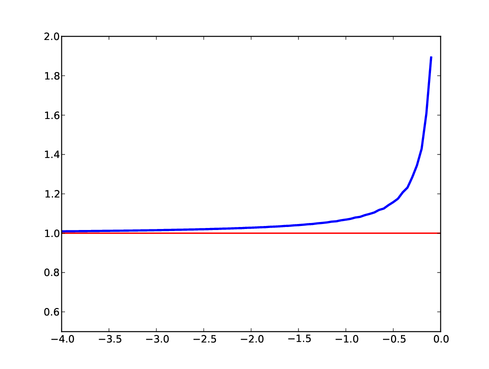
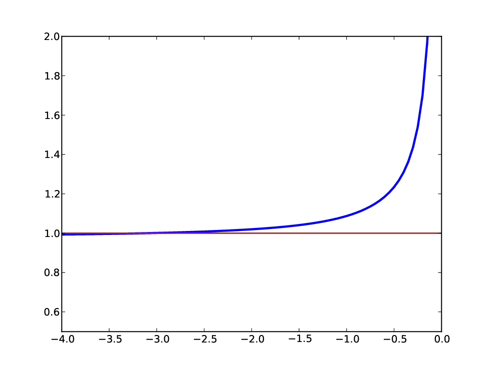
Refer to caption
(a) t=0.25t=0.25
Refer to caption
(b) t=1t=1
Refer to caption
(c) t=3t=3
Refer to caption
(d) t=10t=10
Figure 1: Illustration of the convergence result in Theorem 4.6 for the Stein–Stein model in the case y<0y<0 (left ‘wing’ of the local volatility). The blue line shows the value of the function y↦σloc2​(y,t)/(y×zt​(−1)2)y\mapsto\sigma_{\text{loc}}^{2}(y,t)/(y\times z_{t}(-1)^{2}), with zt​(−1)2z_{t}(-1)^{2} the theoretical asymptotic value in (4.21), which must converge to 11 as y→−∞y\to-\infty. Model parameters: a=0,b=−0.5,c=0.4,z0=0.244,ρ=−0.75a=0,b=-0.5,c=0.4,z_{0}=0.244,\rho=-0.75.
Refer to caption
(a) t=0.25t=0.25
Refer to caption
(b) t=1t=1
Refer to caption
(c) t=3t=3
Refer to caption
(d) t=10t=10
Figure 2: Illustration of the convergence result in Theorem 4.6 for the Stein–Stein model in the case y>0y>0 (right ‘wing’ of the local volatility). The blue line shows the value of the function y↦σloc2​(y,t)/(y×zt​(1)2)y\mapsto\sigma_{\text{loc}}^{2}(y,t)/(y\times z_{t}(1)^{2}), with zt​(1)2z_{t}(1)^{2} the theoretical asymptotic value in (4.21), which must converge to 11 as y→∞y\to\infty. Model parameters: a=0,b=−0.5,c=0.4,z0=0.244,ρ=−0.75a=0,b=-0.5,c=0.4,z_{0}=0.244,\rho=-0.75.

Appendix A Technical proofs

A.1 Localization

Here we define the precise localization procedure for the SDE (4.3) that is used in Theorem 4.2, and state the lemma about the localization of the action that is used therein. Consider a family of truncation functions ψR∈Cb∞​(ℝ,ℝ)\psi_{R}\in C^{\infty}_{b}(\mathbb{R};\mathbb{R}), R>0R>0, such that

ψR​(x)={xif ​|x|≤RR+1if ​|x|≥R+1\psi_{R}(x)=\left\{\begin{array}[]{l l}x&\mbox{if }|x|\leq R\\ R+1&\mbox{if }|x|\geq R+1\end{array}\right.

and set

βεR​(x)=bε​(ψR​(x));β0R=β0​(ψR​(x));αR=α⁡(ψR​(x));\beta_{\varepsilon}^{R}(x)=b_{\varepsilon}(\psi_{R}(x));\quad\beta_{0}^{R}=\beta_{0}(\psi_{R}(x));\quad\alpha^{R}=\alpha(\psi_{R}(x)); (A.1)

so that for every RR, the truncated vector fields βεR,β0R\beta_{\varepsilon}^{R},\beta_{0}^{R} and αR\alpha^{R} coincide with the original ones on the ball BR​(0)B_{R}(0), but they remain bounded on ℝn\mathbb{R}^{n} (uniformly in ε\varepsilon in the case of βεR\beta_{\varepsilon}^{R}, thanks to assumption (4.4)). If KK is a common Lipschitz constant for b0b_{0} and α\alpha, then

Lip(b0R)≤K;Lip(αR)≤K,for all RLip(b_{0}^{R})\leq K;\qquad Lip(\alpha^{R})\leq K,\qquad\mbox{for all }R (A.2)

and it is clear that αR​(0)=α⁡(0)≠0\alpha^{R}(0)=\alpha(0)\neq 0 under assumption (SV). It follows that strong Hörmander condition (sH) holds at all points also for the controlled system with truncated coefficients

d​ytR​(h)\displaystyle dy^{R}_{t}(h) =−121θ=0(zRt(h))2dt+zRt(h)dh¯1t,yR0(h)=0,\displaystyle=-\frac{1}{2}1_{\theta=0}\bigl(z^{R}_{t}(h)\bigr)^{2}dt+z^{R}_{t}(h)d\overline{h}^{1}_{t},\quad y^{R}_{0}(h)=0, (A.3)
d​ztR​(h)\displaystyle dz^{R}_{t}(h) =β0R​(ztR​(h))​d​t+αR​(ztR​(h))​d​h¯t2,z0R​(h)=z0\displaystyle=\beta_{0}^{R}(z^{R}_{t}(h))dt+\alpha^{R}(z^{R}_{t}(h))d\overline{h}^{2}_{t},\quad z^{R}_{0}(h)=z_{0}

where h¯=Γ​h\overline{h}=\sqrt{\Gamma}h. Denote ΛtR​(x)=inf{12​|h|H2:h∈𝒦tx​(R)}\Lambda_{t}^{R}(x)=\inf\{\frac{1}{2}|h|_{H}^{2}:h\in\mathcal{K}_{t}^{x}(R)\}, x∈ℝ2x\in\mathbb{R}^{2}, the action of the system (A.3), with 𝒦tx(R)={h∈H:(y0R,z0R)=x0,(ytR,ztR)=x}\mathcal{K}_{t}^{x}(R)=\{h\in H:(y^{R}_{0},z^{R}_{0})=x_{0},(y^{R}_{t},z^{R}_{t})=x\}.

Lemma A.1.

Assume β0\beta_{0} and α\alpha are Lipschitz continuous on ℝn\mathbb{R}^{n}. Denote φ⁡(h)=(y⁡(h),z⁡(h))\varphi(h)=(y(h),z(h)) the solution to the ODE (4.5), and ΛtS​V\Lambda^{SV}_{t} the related action as in (4.6). For every R>0R>0, define b0Rb_{0}^{R} and αR\alpha^{R} according to (A.1), the corresponding ODE solution φR​(h)=(yR​(h),zR​(h))\varphi^{R}(h)=(y^{R}(h),z^{R}(h)) as in (A.3), and the related action ΛtR\Lambda_{t}^{R}. Let y∈ℝly\in\mathbb{R}^{l} and t>0t>0 be fixed as in Theorem 4.2. Then, if at least one of Conditions (i)(i) and (i​i)(ii) of Theorem 4.2 is satisfied:

  • (a)

    for every R>0R>0, there exists R¯​(R)>0\overline{R}(R)>0 such that

    ΛtR¯​(R)​(y,z)=ΛtS​V​(y,z)∀|z|≤R.\Lambda^{\overline{R}(R)}_{t}(y,z)=\Lambda^{SV}_{t}(y,z)\qquad\forall\>|z|\leq R.
  • (b)

    There exists R~>0\tilde{R}>0 such that the maps z↦ΛtS​V​(y,z)z\mapsto\Lambda^{SV}_{t}(y,z) and z↦ΛtR~​(y,z)z\mapsto\Lambda_{t}^{\tilde{R}}(y,z) attain their (common) global minimum at the same points:

    {z∈ℝn−l:ΛtS​V​(y,z)=ΛtS​V​(Ny)}={z∈ℝn−l:ΛtR~​(y,z)=ΛtR~​(Ny)=ΛtS​V​(Ny)}.\{z\in\mathbb{R}^{n-l}:\Lambda^{SV}_{t}(y,z)=\Lambda^{SV}_{t}(N_{y})\}=\{z\in\mathbb{R}^{n-l}:\Lambda_{t}^{\tilde{R}}(y,z)=\Lambda_{t}^{\tilde{R}}(N_{y})=\Lambda^{SV}_{t}(N_{y})\}.

Proof. Arguing as in the proof of Theorem 4.2, if at least one of Conditions (i)(i) or (i​i)(ii) is satisfied, the deterministic Malliavin matrix C(0,z0)​(h)C_{(0,z_{0})}(h) is invertible for all h∈𝒦t(y,⋅)h\in\mathcal{K}_{t}^{(y,\cdot)}; it then follows from Lemma 2.7(v)(v) that Λt\Lambda_{t} is continuous on an open set of ℝ2\mathbb{R}^{2} containing the line Ny=(y,⋅)N_{y}=(y,\cdot).

Let us prove (a)(a). Fix R>0R>0, and define ℋR={h∈H:12​|h|H2≤sup|x|≤RΛtS​V​(x)}\mathcal{H}_{R}=\Bigl\{h\in H:\frac{1}{2}|h|_{H}^{2}\leq\sup_{|x|\leq R}\Lambda^{SV}_{t}(x)\Bigr\}. Since Λt(S​V)\Lambda_{t}^{(SV)} is finite and continuous around NyN_{y}, sup|z|≤RΛtS​V​(y,z)\sup_{|z|\leq R}\Lambda^{SV}_{t}(y,z) is finite and ℋR\mathcal{H}_{R} is bounded in HH. Denote 𝒦m​i​nx\mathcal{K}^{x}_{min} the set of minimizing controls in 𝒦tx\mathcal{K}^{x}_{t}. It is clear that, for every z∈BR​(0)z\in B_{R}(0), 𝒦m​i​n(y,z)⊂ℋR\mathcal{K}^{(y,z)}_{min}\subset\mathcal{H}_{R}, hence ΛtS​V​(y,z)=inf{12​|h|H2:h∈𝒦t(y,z)∩ℋR}\Lambda^{SV}_{t}(y,z)=\inf\Bigl\{\frac{1}{2}|h|_{H}^{2}:h\in\mathcal{K}_{t}^{(y,z)}\cap\mathcal{H}_{R}\Bigr\}, and {y}×BR​(0)⊂{φt​(h):h∈ℋR}\{y\}\times B_{R}(0)\subset\{\varphi_{t}(h):h\in\mathcal{H}_{R}\}. Setting

C​exp⁡(C​suph∈ℋR|h(2)|)≤C​exp⁡(C​(2​sup|z|≤RΛtS​V​(y,z))1/2):=R¯​(R)C\exp\Bigl(C\sup_{h\in\mathcal{H}_{R}}|h^{(2)}|\Bigr)\leq C\exp\Bigl(C\Bigl(2\sup_{|z|\leq R}\Lambda^{SV}_{t}(y,z)\Bigr)^{1/2}\Bigr):=\overline{R}(R)

where C=C⁡(t,z0,K)C=C(t,z_{0},K) is the constant defined in Lemma 2.7(i)(i) and KK is a Lipschitz constant for β0\beta_{0} and α\alpha, it follows from estimate (2.8) that sups≤t|zs​(h)|≤R¯​(R)\sup_{s\leq t}|z_{s}(h)|\leq\overline{R}(R) for every h∈ℋRh\in\mathcal{H}_{R}. Therefore, for such hh the trajectory s↦zs​(h)s\mapsto z_{s}(h), s≤ts\leq t, remains in the region where the vector fields b0,σjb_{0},\sigma_{j} and b0R¯​(R),σjR¯​(R)b^{\overline{R}(R)}_{0},\sigma^{\overline{R}(R)}_{j} coincide: from the uniqueness of solutions for the second ODE in (4.5), it follows that zsR¯​(R)=zsz^{\overline{R}(R)}_{s}=z_{s} for all s∈[0,t]s\in[0,t]. Since y⁡(h)y(h) only depends on z⁡(h)z(h), one also has ysR¯​(R)​(h)=ys​(h)y^{\overline{R}(R)}_{s}(h)=y_{s}(h) for all s≤ts\leq t, hence φtR¯​(R)​(h)=φt​(h)\varphi^{\overline{R}(R)}_{t}(h)=\varphi_{t}(h) for all h∈ℋRh\in\mathcal{H}_{R}. In particular, φtR¯​(R)​(h0)=φt​(h0)\varphi^{\overline{R}(R)}_{t}(h_{0})=\varphi_{t}(h_{0}) for h0∈𝒦min(y,z)h_{0}\in\mathcal{K}_{\min}^{(y,z)}, and this establishes

ΛtR¯​(R)​(y,z)≤12​|h0|2=ΛtS​V​(y,z),∀z∈BR​(0).\Lambda_{t}^{\overline{R}(R)}(y,z)\leq\frac{1}{2}|h_{0}|^{2}=\Lambda^{SV}_{t}(y,z),\qquad\forall z\in B_{R}(0). (A.4)

On the other hand, ΛtR¯​(R)​(y,z)=12​|h¯0|2\Lambda_{t}^{\overline{R}(R)}(y,z)=\frac{1}{2}|\overline{h}_{0}|^{2} for some h¯0∈𝒦(y,z)​(R¯​(R))\overline{h}_{0}\in\mathcal{K}^{(y,z)}(\overline{R}(R)): from (A.4), h¯0∈ℋR\overline{h}_{0}\in\mathcal{H}_{R}, therefore φt​(h¯0)=φtR¯​(R)​(h¯0)=(y,z)\varphi_{t}(\overline{h}_{0})=\varphi^{\overline{R}(R)}_{t}(\overline{h}_{0})=(y,z) by the uniqueness argument above. This implies h¯0∈𝒦(y,z)\overline{h}_{0}\in\mathcal{K}^{(y,z)} and ΛtS​V​(y,z)≤12​|h¯0|2=ΛtR¯​(R)​(y,z)\Lambda^{SV}_{t}(y,z)\leq\frac{1}{2}|\overline{h}_{0}|^{2}=\Lambda_{t}^{\overline{R}(R)}(y,z), and (a)(a) is proved.

Let us now prove (b)(b): note that estimate (2.8) in Lemma 2.7, together with the bound (A.2) on the Lipschitz constants of β0R\beta_{0}^{R} and αR\alpha^{R}, implies

sups≤t|zs​(h)|∨sups≤t|zsR​(h)|≤C​eC​|h|H,∀R\sup_{s\leq t}|z_{s}(h)|\vee\>\sup_{s\leq t}|z^{R}_{s}(h)|\leq Ce^{C|h|_{H}},\qquad\forall\>R (A.5)

where again C=C⁡(t,z0,K)C=C(t,z_{0},K). Set R1=C​exp⁡(C​(2​(ΛtS​V​(Ny)+1))1/2)R^{1}=C\exp\Bigl(C\Bigl(2(\Lambda_{t}^{SV}(N_{y})+1)\Bigr)^{1/2}\Bigr). Estimate (A.5) yields the inclusion {z∈ℝn:ΛtS​V​(y,z)≤ΛtS​V​(Ny)+1}⊆BR1​(0)\{z\in\mathbb{R}^{n}:\Lambda_{t}^{SV}(y,z)\leq\Lambda^{SV}_{t}(N_{y})+1\}\subseteq B_{R^{1}}(0), because for every zz on the left hand side there exists h0h_{0} with 12​|h0|2=ΛtS​V​(y,z)≤ΛtS​V​(Ny)+1\frac{1}{2}|h_{0}|^{2}=\Lambda_{t}^{SV}(y,z)\leq\Lambda^{SV}_{t}(N_{y})+1 such that z=zt​(h0)z=z_{t}(h_{0}). In particular, all the points z∗z^{*} are contained in BR1​(0)B_{R^{1}}(0), where z∗z^{*} is a global minimizer of the map z↦ΛtS​V​(y,z)z\mapsto\Lambda^{SV}_{t}(y,z). Now setting R~=R¯​(R1)\tilde{R}=\overline{R}(R^{1}), point (a)(a) of the current lemma entails that ΛtR~\Lambda^{\tilde{R}}_{t} and ΛtS​V\Lambda^{SV}_{t} coincide on {y}×BR1​(0)\{y\}\times B_{R^{1}}(0), therefore they - trivially - attain their common minimum ΛtS​V​(Ny)\Lambda^{SV}_{t}(N_{y}) on {y}×BR1​(0)\{y\}\times B_{R^{1}}(0) at the same points. One has to make sure that ΛR~\Lambda^{\tilde{R}} is strictly above the level ΛtS​V​(Ny)\Lambda^{SV}_{t}(N_{y}) outside {y}×BR1​(0)\{y\}\times B_{R^{1}}(0): but (A.5) ensures that ztR~=z∉BR1​(0)z^{\tilde{R}}_{t}=z\notin B_{R^{1}}(0) can be reached only along controls hh such that 12​|h|H2>ΛtS​V​(Ny)+1\frac{1}{2}|h|_{H}^{2}>\Lambda_{t}^{SV}(N_{y})+1, hence ΛtR~​(y,z)≥ΛtS​V​(Ny)+1\Lambda^{\tilde{R}}_{t}(y,z)\geq\Lambda_{t}^{SV}(N_{y})+1 for z∉BR1​(0)z\notin B_{R^{1}}(0), and this allows to conclude.  

A.2 Proofs of Theorem 2.1 and Proposition 2.4

The following lemma plays a key role. The proof is given under weak Hörmander condition at the starting point x0x_{0}:

(wH)span{σ1,…,σd;\displaystyle\text{(wH)}\qquad\text{span}\{\sigma_{1},\dots,\sigma_{d}; [b0,σi]:1≤i≤d;[σi,σj]:1≤i,j≤d;\displaystyle[b_{0},\sigma_{i}]:1\leq i\leq d;\ [\sigma_{i},\sigma_{j}]:1\leq i,j\leq d; (A.6)
[[σi,[σl,σm]]:1≤i,l,m≤d;…}|x0=ℝn\displaystyle[[\sigma_{i},[\sigma_{l},\sigma_{m}]]:1\leq i,l,m\leq d;\dots\}\bigr|_{x_{0}}=\mathbb{R}^{n}

that is, the linear span of σ1,…,σd\sigma_{1},\dots,\sigma_{d} and all the Lie brackets of b0,σ1,…,σdb_{0},\sigma_{1},\dots,\sigma_{d} is the whole ℝn\mathbb{R}^{n} at x0x_{0}. Notice that under assumptions (1.7) and (1.13), one has

[bε,σj]x0ε=[b0,σj]x0+o⁡(1),[σj,σk]x0ε=[σj,σk]x0+o⁡(1)[b_{\varepsilon},\sigma_{j}]_{x_{0}^{\varepsilon}}=[b_{0},\sigma_{j}]_{x_{0}}+o(1),\qquad[\sigma_{j},\sigma_{k}]_{x_{0}^{\varepsilon}}=[\sigma_{j},\sigma_{k}]_{x_{0}}+o(1)

hence (wH) also holds when b0b_{0} and x0x_{0} are replaced with bεb_{\varepsilon} and x0εx_{0}^{\varepsilon}, when ε\varepsilon is small enough. It is then classical that XtεX^{\varepsilon}_{t} admits a smooth density ptεp_{t}^{\varepsilon} for all t>0t>0 under condition (wH).

Lemma A.2.

Let XεX^{\varepsilon} be the solution to (1.3). Assume weak Hörmander condition (wH) at x0x_{0}. Then, for any t>0t>0, any x∈ℝnx\in\mathbb{R}^{n} and q∈(0,1)q\in(0,1) there exist a constant CqC_{q} and positive integers N1​(q)=N1​(q,n)N_{1}(q)=N_{1}(q,n) and N⁡(q)=N⁡(q,n,x0)N(q)=N(q,n,x_{0}) such that

ptε(x)≤Cq(1+R−N1​(q))ε−N⁡(q)ℙ(|Xtε−x|≤R)qp^{\varepsilon}_{t}(x)\leq C_{q}\bigl(1+R^{-N_{1}(q)}\bigl)\ \varepsilon^{-N(q)}\ \mathbb{P}(|X^{\varepsilon}_{t}-x|\leq R)^{q} (A.7)

for every R>0R>0. The constant CqC_{q} also depends on tt and on the bounds on the derivatives of b0b_{0} and the (σj)j(\sigma_{j})_{j}.

Proof. Given in section A.3.  

Proof of Theorem 2.1. Let us write Λ\Lambda for the action function throughout this proof (dropping the fixed index tt from the notation). The following estimate is obtained with standard uniform large deviations arguments (see also Léandre [34, section 2]): for every R>0R>0, one has

lim supε→0ε2​log⁡ℙ⁡(|Xtε−x|≤R)≤−Λ⁡(BR​(x))\limsup_{\varepsilon\to 0}\varepsilon^{2}\log\mathbb{P}(|X^{\varepsilon}_{t}-x|\leq R)\leq-\Lambda(B_{R}(x)) (A.8)

uniformly over xx in compact sets.

Let first prove (2.2). xx is fixed; taking lim supε→0ε2​log\limsup_{\varepsilon\to 0}\varepsilon^{2}\log in estimate (A.7) and applying (A.8), one has

lim supε→0ε2​log⁡ptε​(x)≤q​lim supε→0ε2​log⁡ℙ⁡(|Xtε−x|≤R)≤−q​Λ​(BR​(x)).\limsup_{\varepsilon\to 0}\varepsilon^{2}\log p^{\varepsilon}_{t}(x)\leq q\limsup_{\varepsilon\to 0}\varepsilon^{2}\log\mathbb{P}(|X^{\varepsilon}_{t}-x|\leq R)\leq-q\Lambda(B_{R}(x)).

Now taking the limit R→0R\to 0, Λ⁡(BR​(x))=infy∈BR​(x)Λ⁡(y)→Λ⁡(x)\Lambda(B_{R}(x))=\inf_{y\in B_{R}(x)}\Lambda(y)\to\Lambda(x) by the lower semi-continuity of Λ\Lambda. Since q<1q<1 was arbitrary, (2.2) follows.

Let us now prove (2.5). Under the assumption in Theorem 2.1(i​i)(ii), it follows from Lemma 2.7(i​i​i)(iii) that Λ\Lambda is continuous on an open neighborhood VV of xx, hence uniformly continuous on compact sets contained in VV. Fix a compact ball B⊂VB\subset V and δ>0\delta>0. We can find R=RB,δR=R_{B,\delta} such that the closed RR-neighborhood of BB, BR=∪y∈BBR(y)B^{R}=\cup_{y\in B}B_{R}(y), is contained in VV and moreover O​s​c​(Λ,BR​(y))≤δOsc(\Lambda,B_{R}(y))\leq\delta for all y∈By\in B. In particular,

Λ⁡(BR​(y))=infz∈BR​(y)Λ⁡(z)≥Λ⁡(y)−δ\Lambda(B_{R}(y))=\inf_{z\in B_{R}(y)}\Lambda(z)\geq\Lambda(y)-\delta (A.9)

for all y∈By\in B. Now taking lim supε→0ε2​log\limsup_{\varepsilon\to 0}\varepsilon^{2}\log in estimate (A.7), and applying (A.8) and (A.9), it follows that for any q∈(0,1)q\in(0,1)

lim supε→0ε2​log⁡ptε​(y)≤q​lim supε→0ε2​log⁡ℙ⁡(|Xtε−y|≤R)≤−q​Λ​(BR​(y))≤−q⁡(Λ⁡(y)−δ)\limsup_{\varepsilon\to 0}\varepsilon^{2}\log p^{\varepsilon}_{t}(y)\leq q\limsup_{\varepsilon\to 0}\varepsilon^{2}\log\mathbb{P}(|X^{\varepsilon}_{t}-y|\leq R)\leq-q\Lambda(B_{R}(y))\leq-q(\Lambda(y)-\delta)

where the limit holds uniformly over y∈By\in B. Since q<1q<1 and δ\delta were arbitrary, the right hand side can be improved to Λ⁡(y)\Lambda(y), and (2.5) follows.

The lower bound (2.3) is actually estimate (3.5) in Ben Arous and Léandre [6, Theorem III.1]. Their proof can be adapted to the case where bb and x0x_{0} depend on ε\varepsilon, under the convergence conditions (1.7) et (1.13). The statement about Λ=ΛR\Lambda=\Lambda_{R} in Theorem 2.1(i)(i) is obvious from the definitions of the two actions, and (2.4) is a direct consequence of (2.2) and (2.3).  

Proof of Proposition 2.4. It follows from Lemma A.2 that, for every q,q′∈(0,1)q,q^{\prime}\in(0,1) and RR small enough,

∫|z−z¯|≥A|z|k​ptε​(y,z)​𝑑z≤Cq​R−N1​(q)​ε−N⁡(q)​∫|z−z¯|≥A|z|k​ℙ​(|Xtε−(y,z)|≤R)q​𝑑z=Cq​R−N1​(q)​ε−N⁡(q)​∫|z−z¯|≥A|z|k​ℙ​(|Xtε−(y,z)|≤R)q​q′​ℙ​(|Xtε−(y,z)|≤R)q⁡(1−q′)​dz.\int_{|z-\overline{z}|\geq A}|z|^{k}p^{\varepsilon}_{t}(y,z)dz\leq C_{q}R^{-N_{1}(q)}\varepsilon^{-N(q)}\int_{|z-\overline{z}|\geq A}|z|^{k}\mathbb{P}(|X^{\varepsilon}_{t}-(y,z)|\leq R)^{q}dz\\ =C_{q}R^{-N_{1}(q)}\varepsilon^{-N(q)}\int_{|z-\overline{z}|\geq A}|z|^{k}\mathbb{P}(|X^{\varepsilon}_{t}-(y,z)|\leq R)^{qq^{\prime}}\>\mathbb{P}(|X^{\varepsilon}_{t}-(y,z)|\leq R)^{q(1-q^{\prime})}dz.

Since

ℙ⁡(|Xtε−(y,z)|≤R)\displaystyle\mathbb{P}(|X^{\varepsilon}_{t}-(y,z)|\leq R) ≤ℙ⁡(|Ytε−y|≤R,|Ztε−z|≤R)\displaystyle\leq\mathbb{P}(|Y^{\varepsilon}_{t}-y|\leq R,|Z^{\varepsilon}_{t}-z|\leq R)

one has

∫|z−z¯|≥A|z|k​ptε​(y,z)​𝑑z≤Cq​R−N1​(q)​ε−N⁡(q)×ℙ​(|Ytε−y|≤R,|Ztε−z¯|≥A−R)q​q′×∫|z−z¯|≥A|z|k​ℙ​(|Ztε−z|≤R)q⁡(1−q′)​dz.\int_{|z-\overline{z}|\geq A}|z|^{k}p^{\varepsilon}_{t}(y,z)dz\leq C_{q}\>R^{-N_{1}(q)}\varepsilon^{-N(q)}\times\mathbb{P}(|Y^{\varepsilon}_{t}-y|\leq R,|Z^{\varepsilon}_{t}-\overline{z}|\geq A-R)^{qq^{\prime}}\\ \times\int_{|z-\overline{z}|\geq A}|z|^{k}\mathbb{P}(|Z^{\varepsilon}_{t}-z|\leq R)^{q(1-q^{\prime})}dz. (A.10)

The integral on the right hand side of (A.10) can be bounded as follows

∫|z−z¯|≥A|z|k​ℙ​(|Ztε−z|≤R)q⁡(1−q′)​𝑑z≤∫ℝn−l|z|k​ℙ​(|Ztε|≥|z|−R)q⁡(1−q′)​𝑑z.\int_{|z-\overline{z}|\geq A}|z|^{k}\mathbb{P}(|Z^{\varepsilon}_{t}-z|\leq R)^{q(1-q^{\prime})}dz\leq\int_{\mathbb{R}^{n-l}}|z|^{k}\mathbb{P}(|Z^{\varepsilon}_{t}|\geq|z|-R)^{q(1-q^{\prime})}dz. (A.11)

Note that the random variable |Ztε||Z^{\varepsilon}_{t}| has moment of all orders uniformly bounded in ε\varepsilon (for so does |Xtε||X^{\varepsilon}_{t}|): precisely, for any T>0T>0 and r>0r>0 there exists a constant Cr=Cr,TC_{r}=C_{r,T} such that supε≤1𝔼⁡[(Ztε)r]≤Cr\sup_{\varepsilon\leq 1}\>\mathbb{E}[(Z^{\varepsilon}_{t})^{r}]\leq C_{r} for all t≤Tt\leq T. Then, from Markov’s inequality

supε≤1ℙ⁡(|Ztε|≥|z|−2​R)≤Cr(|z|−R)r\sup_{\varepsilon\leq 1}\>\mathbb{P}(|Z^{\varepsilon}_{t}|\geq|z|-2R)\leq\frac{C_{r}}{(|z|-R)^{r}} (A.12)

for all zz such that |z|−R>0|z|-R>0 and all r>0r>0. The exponent rr can be chosen sucht that

supε≤1ℙ​(|Ztε|≥|z|−R)q⁡(1−q′)≤C(1)|z|k+n−l+1,\sup_{\varepsilon\leq 1}\mathbb{P}(|Z^{\varepsilon}_{t}|\geq|z|-R)^{q(1-q^{\prime})}\leq\frac{C^{(1)}}{|z|^{k+n-l+1}},

for all |z||z| larger than, say, 1+R1+R, for some positive constant C(1)=CT(1)C^{(1)}=C^{(1)}_{T}. It follows that for any choice of q,q′∈(0,1)q,q^{\prime}\in(0,1), the integral on the right hand side of (A.11) is convergent, and uniformly bounded in ε\varepsilon.

Finally taking log\log, multiplying by ε2\varepsilon^{2} and taking lim supε→0\limsup_{\varepsilon\to 0} in (A.10), we have

lim supε→0ε2​log​∫|z−z¯|≥A|z|k​ptε​(y,z)​dz≤q​q′​lim supε→0ε2​log⁡ℙ⁡(|Ytε−y|≤R,|Ztε−z¯|≥A−R)≤−qq′inf{Λt(y′,z′):|y′−y|≤R,|z′−z¯|≥A−R}.\limsup_{\varepsilon\to 0}\varepsilon^{2}\log\int_{|z-\overline{z}|\geq A}|z|^{k}p^{\varepsilon}_{t}(y,z)dz\leq qq^{\prime}\>\limsup_{\varepsilon\to 0}\varepsilon^{2}\log\mathbb{P}(|Y^{\varepsilon}_{t}-y|\leq R,|Z^{\varepsilon}_{t}-\overline{z}|\geq A-R)\\ \leq-qq^{\prime}\>\inf\{\Lambda_{t}(y^{\prime},z^{\prime}):|y^{\prime}-y|\leq R,|z^{\prime}-\overline{z}|\geq A-R\}.

As R↓0R\downarrow 0, the right hand side tends to −qq′inf{Λt(y,z′):|z′−z¯|≥A}-qq^{\prime}\>\inf\{\Lambda_{t}(y,z^{\prime}):|z^{\prime}-\overline{z}|\geq A\}: since q,q′<1q,q^{\prime}<1 were arbitrary, we obtain the claim.  

A.3 Proof of Lemma A.2

Throughout this section, we denote X=(Xt,t≥0)X=(X_{t};t\geq 0) the strong solution of the SDE

Xt=x0+∫0tB⁡(Xs)​𝑑s+∑j=1d∫0tAj​(Xs)​d​Wsj,t≥0X_{t}=x_{0}+\int_{0}^{t}B(X_{s})ds+\sum_{j=1}^{d}\int_{0}^{t}A_{j}(X_{s})dW^{j}_{s},\ \ \ t\geq 0 (A.13)

where B,Aj∈𝒞b∞​(ℝn,ℝn)B,A_{j}\in\mathcal{C}^{\infty}_{b}(\mathbb{R}^{n};\mathbb{R}^{n}) for all jj. For any multi-index α=(α1,…,αl)∈{1,…,n}l\alpha=(\alpha_{1},\dots,\alpha_{l})\in\{1,\dots,n\}^{l}, we denote |α|=l|\alpha|=l and ∂α=∂|α|xα1,…,xαl\partial_{\alpha}=\partial^{|\alpha|}_{x_{\alpha_{1}},\dots,x_{\alpha_{l}}}. Setting

|f|k=∑|α|≤ksupy∈ℝn|∂αf⁡(y)||f|_{k}=\sum_{|\alpha|\leq k}\sup_{y\in\mathbb{R}^{n}}|\partial_{\alpha}f(y)|

for smooth real valued functions ff, we denote _​k=1+∑i=1n|Bi|k\hbox{_}k=1+\sum_{i=1}^{n}|B^{i}|_{k} and |A|k=1+∑i,j|Aji|k|A|_{k}=1+\sum_{i,j}|A^{i}_{j}|_{k}.

Some elements of Malliavin calculus. Following the standard notation in [38], we denote 𝔻k,p\mathbb{D}^{k,p} the domain of the kk-th order Malliavin derivative, and 𝔻∞=∩k≥1∩p≥1𝔻k,p\mathbb{D}^{\infty}=\cap_{k\geq 1}\cap_{p\geq 1}\mathbb{D}^{k,p}. It is classical, see [38], that XtX_{t} is a smooth random variable in Malliavin’s sense for every tt, that is Xt∈𝔻∞X_{t}\in\mathbb{D}^{\infty}. Denoting Dr​Xt=(Dr1​Xt,…,Drd​Xt)D_{r}X_{t}=(D_{r}^{1}X_{t},\dots,D_{r}^{d}X_{t}), r∈[0,t]r\in[0,t] the (dd-dimensional) Malliavin derivative of XtX_{t}, the kk-th order derivative is obtained by iterating the operator: Dj1,…,jkr1,…​rkXt:=Dr1j1⋯DrkjkXtD^{j_{1},\dots,j_{k}}_{r_{1},\dots r_{k}}X_{t}:=D_{r_{1}}^{j_{1}}\cdots D_{r_{k}}^{j_{k}}X_{t}, for every (j1,…,jk)∈{1,…,d}k(j_{1},\dots,j_{k})\in\{1,\dots,d\}^{k}. It is well-known that the random variables Dr1,…,rkj1,…,jk​XtD^{j_{1},\dots,j_{k}}_{r_{1},\dots,r_{k}}X_{t} have finite moments of any order: the following lemma gives an explicit estimate on the LpL^{p} norms, in terms of the bounds on AA and BB and their derivatives, and will be useful in what follows.

Lemma A.3 (Lemma 2.1 and Corollary 1 in [10]).

For every k≥1k\geq 1 and p>1p>1 there exist positive integers γ,γ′\gamma,\gamma^{\prime} and a positive constant CC, all depending on k,pk,p but not on the bounds on BB and AA and their derivatives, such that, for any t>0t>0

supr1,…,rk≤t𝔼⁡[|Dr1,…,rkj1,…,jk​X|p]≤Ck,p​(t1/2​_​k+|A|k)γ′​eγ​(t​|B|1+t1/2|​A|1)p\sup_{r_{1},\dots,r_{k}\leq t}\mathbb{E}\left[\left|D^{j_{1},\dots,j_{k}}_{r_{1},\dots,r_{k}}X\right|^{p}\right]\leq C_{k,p}\left(t^{1/2}\hbox{_}k+|A|_{k}\right)^{\gamma^{\prime}}e^{\gamma(t|B|_{1}+t^{1/2}|A|_{1})^{p}}

for all i=1,…,mi=1,\dots,m and (j1,…,jk)∈{1,…,d}k(j_{1},\dots,j_{k})\in\{1,\dots,d\}^{k}. Moreover,

‖ϕ⁡(Xt)‖k,p≤Ck,p​|ϕ|k​(1+(t∨tk)1/2)​(t1/2​_​k+|A|k)γ′​ek​γ​(t​|B|1+t1/2|​A|1)p||\phi(X_{t})||_{k,p}\leq C_{k,p}\>|\phi|_{k}\>\bigl(1+\bigl(t\vee t^{k}\bigr)^{1/2}\bigr)\bigl(t^{1/2}\hbox{_}k+|A|_{k}\bigr)^{\gamma^{\prime}}e^{k\gamma(t|B|_{1}+t^{1/2}|A|_{1})^{p}}

for any ϕ∈C∞​(ℝn)\phi\in C^{\infty}(\mathbb{R}^{n}).

The notion of non-degeneracy for (Malliavin-)differentiable random variables F∈𝔻1,2F\in\mathbb{D}^{1,2} is understood in the sense of the (stochastic) Malliavin covariance matrix

(γF)i,j=∫0t∑l=1dDsl​Fi​Dsl​Fj​𝑑s,i,j=1,…,d.(\gamma_{F})_{i,j}=\int_{0}^{t}\sum_{l=1}^{d}D^{l}_{s}F^{i}\>D^{l}_{s}F^{j}ds,\quad i,j=1,\dots,d.

A fundamental tool to study density of random variables with invertible covariance matrix is the integration by parts formula:

Proposition A.4 (Integration by parts formula of the Malliavin calculus; [38]).

Let F=(F1,…,Fd)∈𝔻∞F=(F^{1},\dots,F^{d})\in\mathbb{D}^{\infty}. Assume that γF\gamma_{F} is invertible a.s. and moreover 𝔼⁡[det(σF)−p]<∞\mathbb{E}[\det(\sigma_{F})^{-p}]<\infty for all p≥1p\geq 1. Let G∈𝔻∞G\in\mathbb{D}^{\infty} and ϕ∈Cpol∞​(ℝm)\phi\in C^{\infty}_{\text{pol}}(\mathbb{R}^{m}). Then, for any k≥1k\geq 1 and any multi-index α=(α1,…,αk)∈{1,…,m}k\alpha=(\alpha_{1},\dots,\alpha_{k})\in\{1,\dots,m\}^{k} there exists a random variable Hα​(F,G)∈𝔻∞H_{\alpha}(F,G)\in\mathbb{D}^{\infty} such that

𝔼⁡[∂αϕ⁡(F)​G]=𝔼⁡[ϕ⁡(F)​Hα​(F,G)],\mathbb{E}\left[\partial_{\alpha}\phi(F)G\right]=\mathbb{E}\left[\phi(F)H_{\alpha}(F,G)\right], (A.14)

where the Hα​(F,G)H_{\alpha}(F,G) are recursively defined by

Hα​(F,G)=H(αk)​(F,H(α1,…,αk−1)​(F,G)),H(i)​(F,G)=∑j=1mδ⁡(G​(σF−1)i,j​D​Fj)H_{\alpha}(F,G)=H_{(\alpha_{k})}(F,H_{(\alpha_{1},\dots,\alpha_{k-1})}(F,G)),\qquad H_{(i)}(F,G)=\sum_{j=1}^{m}\delta\left(G(\sigma_{F}^{-1})_{i,j}DF^{j}\right)

where δ\delta denotes the adjoint operator of DD.

The key ingredient required to apply the integration by parts is an estimate of the LpL^{p} norms of the Malliavin weights HαH_{\alpha}. The following theorem, proved in [10], provides explicit bounds in terms of the bounds on AA and BB and their derivatives.

Theorem A.5 (Theorem 2.3 in [10]).

For every k≥1k\geq 1, there exist a positive constant CkC_{k} and positive integers ak,bk,cka_{k},b_{k},c_{k} and rkr_{k}, all possibly depending also on nn and dd, such that for any multi-index α∈{1,…,n}k\alpha\in\{1,\dots,n\}^{k}, any G∈𝔻∞G\in\mathbb{D}^{\infty} and any t>0t>0,

||Hα(Xt,G)||2≤Ck(1+tk)||G||k,2k+1𝔼[det(γt)−rk]×(|B|k+1+|A|k+1)bke(t⁡(|B|1+|​A|12)+t1/2​|A|1)ck.||H_{\alpha}(X_{t},G)||_{2}\leq C_{k}(1+t^{{}_{k}})\ ||G||_{k,2^{k+1}}\>\mathbb{E}[\det(\gamma_{t})^{-r_{k}}]\\ \times(|B|_{k+1}+|A|_{k+1})^{b_{k}}e^{(t(|B|_{1}+|A|_{1}^{2})+t^{1/2}|A|_{1})^{c_{k}}}.

Let us go back to equation (A.13). If the stochastic integral in (A.13) is intended in Stratonovich sense, the drift coefficient BB is replaced by A0=B−12​∑j=1d∑k=1nAjk​∂xkAjA_{0}=B-\frac{1}{2}\sum_{j=1}^{d}\sum_{k=1}^{n}A^{k}_{j}\partial_{x_{k}}A_{j}. If we assume that the vector field (A0,Aj)(A_{0},A_{j}) satisfy the weak Hörmander condition at x0x_{0}

span{A1,…,Ad;\displaystyle\qquad\text{span}\{A_{1},\dots,A_{d}; [A0,Ai]:1≤i≤d;[Ai,Aj]:1≤i,j≤d;\displaystyle[A_{0},A_{i}]:1\leq i\leq d;\ [A_{i},A_{j}]:1\leq i,j\leq d; (A.15)
[[Ai,[Al,Am]]:1≤i,l,m≤d;…}|x0=ℝn,\displaystyle[[A_{i},[A_{l},A_{m}]]:1\leq i,l,m\leq d;\dots\}\bigr|_{x_{0}}=\mathbb{R}^{n},

then, denoting Vx0LV^{L}_{x_{0}} the vector space spanned by the Lie brackets of length smaller or equal to LL in (A.15), and setting1212 12 The sum in (A.16) is in fact taken over a finite number of generating brackets, and it can alternatively be written using the notation introduced in the Appendix of [32].

𝒱L​(x0,v,A0,A)=∑V∈Vx0L⟨v,V​v⟩2v∈ℝn,\mathcal{V}_{L}(x_{0},v;A_{0},A)=\sum_{V\in V^{L}_{x_{0}}}\langle v,Vv\rangle^{2}\qquad v\in\mathbb{R}^{n}, (A.16)

it follows from (A.15) that there exists some L≥1L\geq 1 such that 𝒱L​(x0,v,A0,A)=0⇒v=0\mathcal{V}_{L}(x_{0},v;A_{0},A)=0\Rightarrow v=0. In other words,

𝒱L​(x0,A0,A)=inf|v|=1𝒱L​(x,v,A0,A)>0\mathcal{V}_{L}(x_{0};A_{0},A)=\inf_{|v|=1}\mathcal{V}_{L}(x,v;A_{0},A)>0

for some L≥1L\geq 1. Under condition (wH) at x0x_{0}, the Malliavin covariance matrix γXt\gamma_{X_{t}} satisfies the fundamental estimate of Kusuoka and Stroock [32, Corollary 3.25]: for every T>0T>0 and r>0r>0, there exist a constant Cr=Cr​(T)C_{r}=C_{r}(T) and an integer N⁡(L,n)N(L,n) such that

𝔼​[det(γt)−r]1/r≤Crtn​L​𝒱L​(x0,A0,A)N⁡(L,n)\mathbb{E}[\det(\gamma_{t})^{-r}]^{1/r}\leq\frac{C_{r}}{t^{nL}\ \mathcal{V}_{L}(x_{0};A_{0},A)^{N(L,n)}} (A.17)

for all t∈(0,T]t\in(0,T].

We are now ready to give the following

Proof of Lemma A.2. Let 1{BR/2​(0)}≤φ¯R≤1{BR​(0)}1_{\{B_{R/2}(0)\}}\leq\overline{\varphi}_{R}\leq 1_{\{B_{R}(0)\}} be a C∞C^{\infty} function. We can construct φ¯R\overline{\varphi}_{R} so that |φ¯R|k≤Ck​(1+R−k)|\overline{\varphi}_{R}|_{k}\leq C_{k}(1+R^{-k}) for some constant CkC_{k} (eventually depending on the dimension nn). Define φR​(y):=φ¯R​(y−x)\varphi_{R}(y):=\overline{\varphi}_{R}(y-x) and consider the Fourier transform of ptε​φRp_{t}^{\varepsilon}\varphi_{R}, that is (up to a constant factor)

p^t,Rε​(ξ):=ptε​φR^​(ξ)=𝔼⁡[ei⁡⟨ξ,Xtε⟩​φR​(Xtε)].\hat{p}_{t,R}^{\varepsilon}(\xi):=\widehat{p_{t}^{\varepsilon}\varphi_{R}}(\xi)=\mathbb{E}[e^{i\langle\xi,X^{\varepsilon}_{t}\rangle}\varphi_{R}(X^{\varepsilon}_{t})].

Since the function y→ptε​(y)​φR​(y)y\to p_{t}^{\varepsilon}(y)\varphi_{R}(y) is C∞C^{\infty} and compactly supported, p^t,Rε\hat{p}_{t,R}^{\varepsilon} is integrable and we can use Fourier inversion in order to write

ptε​(x)=ptε​(x)​φR​(x)=1(2​π)n​∫ℝne−i​⟨ξ,x⟩​p^t,Rε​(ξ)​𝑑ξ.p_{t}^{\varepsilon}(x)=p_{t}^{\varepsilon}(x)\varphi_{R}(x)=\frac{1}{(2\pi)^{n}}\int_{\mathbb{R}^{n}}e^{-i\langle\xi,x\rangle}\hat{p}_{t,R}^{\varepsilon}(\xi)d\xi. (A.18)

On the one hand, it is clear that

|p^t,Rε|≤ℙ⁡(|Xtε−x|≤R).|\hat{p}_{t,R}^{\varepsilon}|\leq\mathbb{P}(|X^{\varepsilon}_{t}-x|\leq R). (A.19)

On the other hand, using ∂x1k…​∂xnkei​⟨ξ,x⟩=ik​n​(∏j=1nξj)k​ei​⟨ξ,x⟩\partial^{k}_{x_{1}}\dots\partial^{k}_{x_{n}}e^{i\langle\xi,x\rangle}=i^{kn}(\prod_{j=1}^{n}\xi^{j})^{k}e^{i\langle\xi,x\rangle}, and applying Theorem A.5, we have

|(1+(∏j=1nξj)k)​p^t,Rε​(ξ)|\displaystyle\Bigl|\Bigl(1+(\prod_{j=1}^{n}\xi^{j})^{k}\Bigr)\hat{p}_{t,R}^{\varepsilon}(\xi)\Bigr| =|(1+(∏j=1nξj)k)​𝔼​[ei⁡⟨ξ,Xtε⟩​φR​(Xtε)]|\displaystyle=\Bigl|\Bigl(1+(\prod_{j=1}^{n}\xi^{j})^{k}\Bigr)\mathbb{E}[e^{i\langle\xi,X^{\varepsilon}_{t}\rangle}\varphi_{R}(X^{\varepsilon}_{t})]\Bigr| (A.20)
≤1+|𝔼⁡[∂αei⁡⟨ξ,Xtε⟩​φR​(Xtε)]|\displaystyle\leq 1+|\mathbb{E}[\partial_{\alpha}e^{i\langle\xi,X^{\varepsilon}_{t}\rangle}\varphi_{R}(X^{\varepsilon}_{t})]|
=1+|𝔼⁡[ei⁡⟨ξ,Xtε⟩​Hα​(Xtε,φR​(Xtε))]|\displaystyle=1+|\mathbb{E}[e^{i\langle\xi,X^{\varepsilon}_{t}\rangle}H_{\alpha}(X^{\varepsilon}_{t},\varphi_{R}(X^{\varepsilon}_{t}))]|
≤1+‖Hα​(Xtε,φR​(Xtε))‖2\displaystyle\leq 1+||H_{\alpha}(X^{\varepsilon}_{t},\varphi_{R}(X^{\varepsilon}_{t}))||_{2}

where α=({1}k,…,{n}k)\alpha=(\{1\}^{k},\dots,\{n\}^{k}). Using Lemma A.3 and the fact that the norms {|bε|k}ε>0\{|b_{\varepsilon}|_{k}\}_{\varepsilon>0} are bounded in ε\varepsilon, it follows that there exist some ε0>0\varepsilon_{0}>0 such that

‖φR​(Xtε)‖n​k,2n​k+1≤Ck​(1+(t∨tk)1/2)​(t1/2​|bε|k+ε|​σ|k)γ′​ek​γ​(t​|bε|1+t1/2​ε|​σ|1)p​(1+R−n​k)≤Ck(1)​(1+R−n​k)||\varphi_{R}(X^{\varepsilon}_{t})||_{nk,2^{nk+1}}\leq C_{k}\bigl(1+\bigl(t\vee t^{k}\bigr)^{1/2}\bigr)\left(t^{1/2}|b_{\varepsilon}|_{k}+\varepsilon|\sigma|_{k}\right)^{\gamma^{\prime}}e^{k\gamma(t|b_{\varepsilon}|_{1}+t^{1/2}\varepsilon|\sigma|_{1})^{p}}(1+R^{-nk})\\ \leq C^{(1)}_{k}(1+R^{-nk}) (A.21)

for every ε<ε0\varepsilon<\varepsilon_{0}, for some constant Ck(1)=Ck(1)​(t,|b0|k,|σ|k)C^{(1)}_{k}=C^{(1)}_{k}(t,|b_{0}|_{k},|\sigma|_{k}).

When the SDE (1.3) is written in Stratonovich form, the drift bεb_{\varepsilon} is replaced by b¯ε=bε−ε2​12​∑j=1d∑k=1nσjk​∂xkσj\overline{b}_{\varepsilon}=b_{\varepsilon}-\varepsilon^{2}\frac{1}{2}\sum_{j=1}^{d}\sum_{k=1}^{n}\sigma^{k}_{j}\partial_{x_{k}}\sigma_{j}. Noting that 𝒱L​(x0ε,v,b¯ε,ε​σ)\mathcal{V}_{L}(x_{0}^{\varepsilon},v;\overline{b}_{\varepsilon},\varepsilon\sigma) contains terms propositional to ε\varepsilon (coming from the brackets [bε,ε​σj]x0ε=ε​[bε,σj]x0ε=ε⁡([b0,σj]x0+o⁡(1))[b_{\varepsilon},\varepsilon\sigma_{j}]_{x_{0}^{\varepsilon}}=\varepsilon[b_{\varepsilon},\sigma_{j}]_{x_{0}^{\varepsilon}}=\varepsilon([b_{0},\sigma_{j}]_{x_{0}}+o(1))) and terms proportional to ε2\varepsilon^{2} (coming from the brackets [ε​σj,ε​σk]x0ε[\varepsilon\sigma_{j},\varepsilon\sigma_{k}]_{x_{0}^{\varepsilon}}), for ε\varepsilon small enough one has

𝒱L​(x0ε,v,b¯ε,ε​σ)≥ε2​𝒱L​(x0,v,b0,σ).\mathcal{V}_{L}(x_{0}^{\varepsilon},v;\overline{b}_{\varepsilon},\varepsilon\sigma)\geq\frac{\varepsilon}{2}\mathcal{V}_{L}(x_{0},v;b_{0},\sigma).

Therefore, 𝒱Lε​(x0):=inf|v|=1𝒱L​(x0ε,v,b¯ε,ε​σ)≥ε2​𝒱L​(x0,b0,σ)\mathcal{V}^{\varepsilon}_{L}(x_{0}):=\inf_{|v|=1}\mathcal{V}_{L}(x_{0}^{\varepsilon},v;\overline{b}_{\varepsilon},\varepsilon\sigma)\geq\frac{\varepsilon}{2}\mathcal{V}_{L}(x_{0};b_{0},\sigma). Under condition (wH), there exist some L≥1L\geq 1 such that 𝒱L​(x0,b0,σ)>0\mathcal{V}_{L}(x_{0};b_{0},\sigma)>0. Then, it follows from estimate (A.17) that for every r>0r>0 and t>0t>0 there exist ε1\varepsilon_{1}, a function of time Cr​(t)C_{r}(t) and an integer N⁡(L,n)N(L,n) such that

𝔼⁡[det(γtε)−r]≤Cr​(t)​ε−r​N​(L,n)\mathbb{E}[\det(\gamma^{\varepsilon}_{t})^{-r}]\leq C_{r}(t)\>\varepsilon^{-rN(L,n)} (A.22)

for every ε<ε1\varepsilon<\varepsilon_{1}, where γtε\gamma^{\varepsilon}_{t} is the Malliavin covariance matrix of XtεX^{\varepsilon}_{t}.

Now, it follows from (A.21), (A.22) and Theorem A.5 that

‖Hα​(Xtε,φR​(Xtε))‖2≤Ck(2)​(1+R−n​k)​ε−Nk1||H_{\alpha}(X^{\varepsilon}_{t},\varphi_{R}(X^{\varepsilon}_{t}))||_{2}\leq C^{(2)}_{k}(1+R^{-nk})\varepsilon^{-N^{1}_{k}} (A.23)

for every ε<ε0∧ε1\varepsilon<\varepsilon_{0}\wedge\varepsilon_{1}, for some constant Ck(2)C^{(2)}_{k} also depending on (t,|b0|k,|σ|k)(t,|b_{0}|_{k},|\sigma|_{k}), where Nk1=rk​N​(L,n)N^{1}_{k}=r_{k}N(L,n) and rkr_{k} is given in Theorem A.5. Plugging (A.23) into (A.20), one obtains a polynomial estimate for p^t,Rε\hat{p}_{t,R}^{\varepsilon}, precisely

p^t,Rε​(ξ)≤Ck(3)​(1+R−n​k)​ε−Nk11+(∏j=1n|ξ|j)k.\hat{p}_{t,R}^{\varepsilon}(\xi)\leq\frac{C^{(3)}_{k}(1+R^{-nk})\varepsilon^{-N^{1}_{k}}}{1+(\prod_{j=1}^{n}|\xi|^{j})^{k}}. (A.24)

Finally, using (A.23) and applying (A.19) and (A.24), for every q∈(0,1)q\in(0,1) we can write

ptε​(x)\displaystyle p_{t}^{\varepsilon}(x) =1(2​π)n​∫ℝne−i​⟨ξ,x⟩​p^t,Rε​(ξ)​𝑑ξ\displaystyle=\frac{1}{(2\pi)^{n}}\int_{\mathbb{R}^{n}}e^{-i\langle\xi,x\rangle}\hat{p}_{t,R}^{\varepsilon}(\xi)d\xi
=1(2​π)n​∫ℝne−i​⟨ξ,x⟩​p^t,Rε​(ξ)q​p^t,Rε​(ξ)1−q​𝑑ξ\displaystyle=\frac{1}{(2\pi)^{n}}\int_{\mathbb{R}^{n}}e^{-i\langle\xi,x\rangle}\hat{p}_{t,R}^{\varepsilon}(\xi)^{q}\ \hat{p}_{t,R}^{\varepsilon}(\xi)^{1-q}d\xi
≤ℙ​(|Xtε−x|≤R)q​(Ck(3)​(1+R−n​k)​ε−Nk1)1−q​∫ℝn1(1+(∏j=1nξj)k)1−q​dξ.\displaystyle\leq\mathbb{P}(|X^{\varepsilon}_{t}-x|\leq R)^{q}\Bigl(C^{(3)}_{k}(1+R^{-nk})\varepsilon^{-N^{1}_{k}}\Bigr)^{1-q}\int_{\mathbb{R}^{n}}\frac{1}{\bigl(1+(\prod_{j=1}^{n}\xi^{j})^{k}\bigr)^{1-q}}d\xi.

Choosing k=k∗k=k^{*} large enough (but only dependent on nn and qq), the last integral is convergent. Then, the final claim is proved, once we have set N1​(q)=⌈n​k∗​(1−q)⌉N_{1}(q)=\lceil nk^{*}(1-q)\rceil and N⁡(q)=⌈Nk∗1​(1−q)⌉N(q)=\lceil N^{1}_{k^{*}}(1-q)\rceil.  

References

  • [1] A. Agrachev and P. W. Lee, Continuity of optimal control costs and its application to weak KAM theory, Calc. Var. Partial Differ. Equ., 39 (2010), pp. 213–232.
  • [2] I. Bailleul, Large deviation principle for bridges of degenerate diffusion processes. Preprint arXiv, available at http://arxiv.org/pdf/1303.2854.pdf, 2013.
  • [3] I. Bailleul, L. Mesnager, and J. Norris, Small time fluctuations for Riemannian and sub-Riemannian diffusions. Preprint, 2013.
  • [4] P. Baldi and L. Caramellino, General Freidlin-Wentzell large deviations and positive diffusions, Statistics and Probability Letters, 81 (2011), pp. 1218–1229.
  • [5] G. Ben Arous, Développement asymptotique du noyau de la chaleur hypoelliptique hors du cut-locus, Annales scientifiques de l’Ecole Normale Supérieure, 4 (1988), pp. 307–331.
  • [6] G. Ben Arous and R. Léandre, Décroissance exponentielle du noyau de la chaleur sur la diagonale (II), Probab. Theory Relat. Fields, 90 (1991), pp. 377–402.
  • [7] H. Berestycki, J. Busca, and I. Florent, Computing the implied volatility in stochastic volatility models, Communications on Pure and Applied Mathematics, LVII (2004), pp. 1352–1373.
  • [8] J.-M. Bismut, Large deviations and the Malliavin calculus, Birkhäuser, Boston, 1984.
  • [9] P. Cannarsa and L. Rifford, Semiconcavity results for optimal control problems admitting no singular minimizing controls, Ann. Inst. H. Poincaré (C) Anal. Non linéaire, 25 (2008), pp. 773–802.
  • [10] S. De Marco, Smoothness and Asymptotic Estimates of densities for SDEs with locally smooth coefficients and applications to square root-type diffusions, Annals of Applied Probability, 4 (2011), pp. 1282–1321.
  • [11] S. De Marco, P. Friz, and S. Gerhold, Rational Shapes of local volatility, Risk, (February 2013), pp. 82–87.
  • [12] J.-D. Deuschel, P. Friz, A. Jacquier, and S. Violante, Marginal density expansions for diffusions and stochastic volatility I: Theoretical foundations, Communications in Pure and Applied Mathematics, (2014), pp. 40–82.
  • [13]  , Marginal density expansions for diffusions and stochastic volatility II: Applications, Communications in Pure and Applied Mathematics, (2014), pp. 321–350.
  • [14] B. Dupire, Pricing with a smile, Risk, (January 1994).
  • [15] P. Friz, C. Bayer, and P. Laurence, On the probability density function of baskets, in Large Deviations and Asymptotic Methods in Finance, Springer Proceedings in Mathematics & Statistics, vol. 110, Springer, 2015.
  • [16] P. Friz and S. Gerhold, Don’t stay local - extrapolation analytics for Dupire’s local volatility, in Large Deviations and Asymptotic Methods in Finance, Springer Proceedings in Mathematics & Statistics, vol. 110, Springer, 2015.
  • [17] P. Friz, S. Gerhold, and M. Yor, How to make Dupire’s local volatility work with jumps, Quantitative Finance, Special Issue: Themed Issue on Financial Models with Jumps, 14 (2014), pp. 1327–1331.
  • [18] M. Fukasawa, Short-time at-the-money skew and rough fractional volatility. Preprint ArXiv http://arxiv.org/abs/1501.06980, 2015.
  • [19] J. Gatheral, E. Hsu, P. Laurence, C. Ouyang, and T. Wang, Asymptotics of implied volatility in local volatility models, Mathematical Finance, 22 (2012), pp. 591–620.
  • [20] J. Gatheral and A. Jacquier, Arbitrage-free svi volatility surfaces, Quantitative Finance, 14 (2014), pp. 59–71.
  • [21] J. Gatheral and T.-H. Wang, The heat-kernel most-likely-path approximation, International Journal of Theoretical and Applied Finance, 15 (2012), p. 1250001.
  • [22] A. Gulisashvili, Asymptotic formulas with error estimates for call pricing functions and the implied volatility at extreme strikes, SIAM Journal on Financial Mathematics, 1 (2010), pp. 609–641.
  • [23] A. Gulisashvili, Analytically Tractable Stochastic Stock Price Models, Springer-Verlag, Berlin-Heidelberg, 2012.
  • [24] I. Gyöngy, Mimicking the one-dimensional marginal distributions of processes having an Itô differential, Probab. Th. Rel. Fields, 71 (1986), pp. 501–516.
  • [25] P. Henry-Labordère, Analysis, geometry, and modeling in finance: Advanced methods in option pricing. Chapman & Hall/CRC, Financial Mathematics Series, 2008.
  • [26] S. Heston, A closed-form solution for options with stochastic volatility with applications to bond and currency options, The Review of Financial Studies, 6 (1993), pp. 327–343.
  • [27] N. Ikeda and S. Watanabe, Stochastic Differential Equations and Diffusion Processes, North-Holland Publishing Co., second ed., 1989.
  • [28] Y. Inahama, Large deviations for rough path lifts of Watanabe’s pullbacks of delta functions, Int. Math. Res. Notices, (2015).
  • [29] V. Jurdjevic, Geometric control theory, Cambridge University Press, Cambridge ; New York, NY, USA, 1997.
  • [30] M. Keller-Ressel, Moment explosions and long-term behavior of affine stochastic volatility models, Mathematical Finance, 21 (2011), pp. 73–98.
  • [31] S. Kusuoka and Y. Osajima, A remark on the asymptotic expansion of density function of Wiener functionals, Journal of Functional Analysis, special issue dedicated to Paul Malliavin, 255 (2008), pp. 2545–2562.
  • [32] S. Kusuoka and D. Stroock, Application of the Malliavin calculus, Part II, Journal of the Faculty of Science of the Univ. of Tokyo Sect IA Math, 32 (1985), pp. 1–76.
  • [33] R. Léandre, Intégration dans la fibre associée à une diffusion dégénérée, Probab. Th. Rel. Fields, 76 (1987), pp. 341–358.
  • [34]  , Majoration en temps petit de la densité d’une diffusion dégénérée, Probability Theory and Related Fields, 74 (1987), pp. 289–294.
  • [35]  , Minoration en temps petit de la densité d’une diffusion dégénérée, Journal of functional analysis, 74 (1987), pp. 399–414.
  • [36] R. W. Lee, The moment formula for implied volatility at extreme strikes, Mathematical Finance, 14 (2004), pp. 469–480.
  • [37] S. Molchanov, Diffusion processes and Riemannian geometry, Russian Mathematical Surveys, 30 (1975), pp. 1–63.
  • [38] D. Nualart, The Malliavin Calculus and Related Topics, Springer-Verlag, 2006.
  • [39] R. Schöbel and J. Zhu, Stochastic volatility with an Ornstein–Uhlenbeck process: An Extension, European Finance Review, 3 (1999), pp. 23–46.
  • [40] E. M. Stein and J. C. Stein, Stock price distribution with stochastic volatility: an analytic approach, Review of Financial Studies, 4 (1991), pp. 727–752.
  • [41] S. Takanobu and S. Watanabe, Asymptotic expansion formulas of the Schilder type for a class of conditional Wiener functional expectations, in Asymptotic Problems in Probability Theory: Wiener Functionals and Asymptotics, K. D. Elworthy and N. Ikeda, eds., Longman, New York, 1992, pp. 194–241.
  • [42] S. Varadhan, Diffusion processes over a small time interval, Comm. Pure Appl. Math., 20 (1967), pp. 659–685.