跳到论文正文
W Papers独立论文阅读器 arXiv:1311.1396 论文正文 计算阅读时间 · 0%
引用这篇论文根据当前论文元数据生成,正式投稿前建议核对。


License: arXiv.org perpetual non-exclusive license
arXiv:1311.1396v2 [math.AP] 21 Mar 2014

Quantum Ergodicity for Point Scatterers on Arithmetic ToriThanks: P.K. was partially supported by grants from the Göran Gustafsson Foundation and the Swedish Research Council.

Pär Kurlberg Address: Department of Mathematics, KTH Royal Institute of Technology, SE-10044
Stockholm, Sweden
Email address: kurlberg@math.kth.se
and Henrik Ueberschär Address: Institut de Physique Théorique, CEA Saclay, 91191 Gif-sur-Yvette Cedex, France. Email address: henrik.uberschar@cea.fr
Date: August 24, 2026
Abstract.

We prove an analogue of Shnirelman, Zelditch and Colin de Verdiè- re’s Quantum Ergodicity Theorems in a case where there is no underlying classical ergodicity. The system we consider is the Laplacian with a delta potential on the square torus. There are two types of wave functions: old eigenfunctions of the Laplacian, which are not affected by the scatterer, and new eigenfunctions which have a logarithmic singularity at the position of the scatterer. We prove that a full density subsequence of the new eigenfunctions equidistribute in phase space. Our estimates are uniform with respect to the coupling parameter, in particular the equidistribution holds for both the weak and strong coupling quantizations of the point scatterer.

1. Introduction

The point scatterer, namely the Laplacian with a delta potential, on a two-dimensional flat manifold is a popular model in the study of the transition between chaos and integrability in quantum systems. In 1990 Seba [14] considered this operator on a rectangle with irrational aspect ratio and Dirichlet boundary conditions and argued that the spectrum and eigenfunctions of the point scatterer display features such as level repulsion and a Gaussian value distribution, both of which are present in quantum systems with chaotic classical dynamics (cf. [4] and [2]), such as the quantization of the geodesic flow on hyperbolic manifolds or the flow in the Sinai billiard. In fact the point scatterer can be understood as a limit of the Sinai billiard where the radius shrinks to zero faster than the semiclassical wavelength.

The subject of this paper is a point scatterer on a flat torus. It has two types of eigenfunctions: first there are old eigenfunctions of the Laplacian, namely those which vanish at the position of the scatterer; the nonzero eigenvalues remain the same, though with multiplicities reduced by 11. Secondly, there are new eigenfunctions which diverge logarithmically near the position of the scatterer; the corresponding eigenvalues have multiplicity 11 and interlace with the old Laplace eigenvalues.

We shall only be concerned with the set of new eigenfunctions, i.e., the ones which are affected by the scatterer. In [11] it was proved that a full density subsequence11 1 See Section 3 for a precise definition of a “full density subsequence”. of the new eigenfunctions equidistribute in position space in the special case of a square torus. We extend the results of [11] and prove that a full density subsequence of these eigenfunctions in fact equidistribute in phase space — we thus establish an analogue of Shnirelman, Zelditch and Colin de Verdière’s Quantum Ergodicity Theorem in a case where there is no underlying chaotic dynamics and no classical ergodicity.

An analogue of this result for a cubic 3D torus was recently obtained by N. Yesha [18]. The situation for a square torus is very different from irrational tori, where the eigenfunctions are expected to localise in phase space on a finite number of momentum vectors [7, 1]. In the case where the aspect ratio is diophantine this can be proven rigorously for a full density subsequence of new eigenfunctions [8].

1.1. Spectrum of the point scatterer

The formal operator

−Δ+α​δx0,α∈ℝ-\Delta+\alpha\delta_{x_{0}},\quad\alpha\in{\mathbb{R}}

is realized using von Neumann’s theory of self-adjoint extensions. We simply state the most important facts in this section in order to formulate the results of this paper. For a more detailed discussion of the self-adjoint realization of the point scatterer we refer the reader to the introduction and appendix of the paper [11].

Let 𝕋2=ℝ2/2​π​ℤ2{\mathbb{T}}^{2}={\mathbb{R}}^{2}/2\pi{\mathbb{Z}}^{2}. We consider the restriction of the positive Laplacian −Δ-\Delta to the domain

D0=Cc∞​(𝕋2∖{x0})D_{0}=C^{\infty}_{c}({\mathbb{T}}^{2}\setminus\{x_{0}\})

of functions which vanish near the position of the scatterer:

H=−Δ|D0H=-\Delta|_{D_{0}}

The operator HH is symmetric, but fails to be self-adjoint, in fact HH has deficiency indices (1,1)(1,1). Self-adjoint extension theory tells us that there exists a one-parameter family of self-adjoint extensions HφH_{\varphi}, φ∈(−π,π]\varphi\in(-\pi,\pi], which are restrictions of the adjoint H∗H^{*} to the domain of functions f∈Dom⁡(H∗)f\in\operatorname{Dom}(H^{*}) which satisfy the asymptotic

f⁡(x)=C⁡(cos⁡(φ2)​log⁡|x−x0|2​π+sin⁡(φ2))+o⁡(1),x→x0f(x)=C\left(\cos\left(\frac{\varphi}{2}\right)\frac{\log|x-x_{0}|}{2\pi}+\sin\left(\frac{\varphi}{2}\right)\right)+o(1),\quad x\to x_{0}

for some constant C∈ℂC\in{\mathbb{C}}. The case φ=π\varphi=\pi corresponds to α=0\alpha=0. In this paper we will study the operators HφH_{\varphi}, φ∈(−π,π)\varphi\in(-\pi,\pi).

The spectrum of the operator HφH_{\varphi} consists of two parts: “old” and“new” eigenvalues. Since HφH_{\varphi} is a self-adjoint realization of a rank one perturbation of the Laplacian, the effect is that each nonzero old Laplace eigenvalue appears, with multiplicity reduced by 11, in the spectrum of HφH_{\varphi}. Further, each old Laplace eigenvalue gives rise to a new eigenvalue with multiplicity 11. In fact, these new eigenvalues interlace with the multiplicity one sequence associated with the old Laplace eigenvalues.

There are two types of eigenfunctions of HφH_{\varphi} associated with the two parts of the spectrum:

  • (A)

    “Old” eigenfunctions which vanish at x0x_{0} and therefore are not affected by the scatterer. These are simply eigenfunctions of the unperturbed Laplacian.

  • (B)

    “New” eigenfunctions which feature a logarithmic singularity at x0x_{0}; in fact they are given by Green’s functions Gλ=(Δ+λ)−1​δx0G_{\lambda}=(\Delta+\lambda)^{-1}\delta_{x_{0}}.

We will study how eigenfunctions of type (B) are distributed in phase space as the eigenvalue tends to infinity. Denote by SS the set of distinct eigenvalues of the Laplacian on 𝕋2{\mathbb{T}}^{2}, namely integers which can be represented as a sum of two squares:

S:={n∈ℤ:n=x2+y2∣x,y∈ℤ}S:=\{n\in{\mathbb{Z}}:n=x^{2}+y^{2}\mid x,y\in{\mathbb{Z}}\}

For given n∈Sn\in S denote its multiplicity by

r2​(n):=∑n=|ξ|2ξ∈ℤ21,r_{2}(n):=\sum_{\begin{subarray}{c}n=|\xi|^{2}\\ \xi\in{\mathbb{Z}}^{2}\end{subarray}}1,

i.e. the number of ways nn can be written as a sum of two squares.

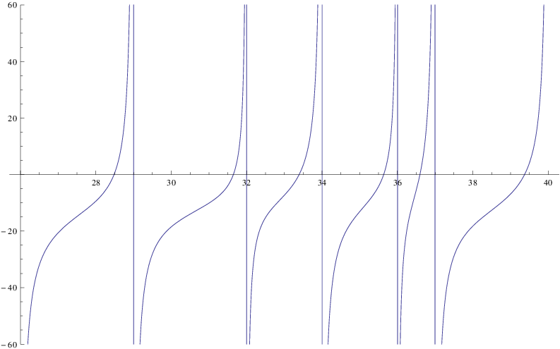
The eigenvalues of type (B) are solutions to the equation
Refer to caption
Figure 1. The picture shows a plot of the l. h. s. of equation (1.1) as a function of λ\lambda. The zeroes are the new eigenvalues corresponding to the self-adjoint extension with parameter φ=0\varphi=0.
(1.1) ∑n∈Sr2​(n)​(1n−λ−nn2+1)=c0​tan⁡(φ2)\sum_{n\in S}r_{2}(n)\left(\frac{1}{n-\lambda}-\frac{n}{n^{2}+1}\right)=c_{0}\tan\left(\frac{\varphi}{2}\right)

(see Figure 1 for a plot of the l. h. s.) where

(1.2) c0=∑n∈Sr2​(n)n2+1.c_{0}=\sum_{n\in S}\frac{r_{2}(n)}{n^{2}+1}.

As mentioned earlier, they interlace with the distinct Laplace eigenvalues

S={0<1<2<4<5<8<⋯}S=\{0<1<2<4<5<8<\cdots\}

as follows

(1.3) λ0,φ<0<λ1,φ<1<λ2,φ<2<λ4,φ<4<λ5,φ<5<λ8,φ<8<⋯\lambda_{0,\varphi}<0<\lambda_{1,\varphi}<1<\lambda_{2,\varphi}<2<\lambda_{4,\varphi}<4<\lambda_{5,\varphi}<5<\lambda_{8,\varphi}<8<\cdots

where the new eigenvalue associated with n∈Sn\in S is denoted by λn,φ\lambda_{n,\varphi}; note that λn,φ<n\lambda_{n,\varphi}<n.

1.2. Strong coupling

In the physics literature equation (1.1) is referred to as a “weak coupling” quantization. In fact, (cf. [12]) the new eigenvalues λm,φ\lambda_{m,\varphi} “clump” with the Laplace eigenvalues m∈Sm\in S in the sense that for a full density subsequence of S,

0<m−λm,φ≪1(log⁡m)1−o⁡(1).0<m-\lambda_{m,\varphi}\ll\frac{1}{(\log m)^{1-o(1)}}.

In particular the eigenvalue spacing distribution of the point scatterer coincides with that of the Laplacian, and the effect of the scatterer on the spectrum is quite weak in this quantization. (In a sense it corresponds to letting α→0\alpha\to 0 as λ→∞\lambda\to\infty.)

Shigehara [15] and later Bogomolny, Gerland and Schmit [3], with the intent of finding a model exhibiting level repulsion, considered another quantization sometimes referred to as a “strong coupling” quantization. There are various ways to arrive at this quantization condition from equation (1.1). For example, one may truncate the summation outside an energy window of size O⁡(λδ)O(\lambda^{\delta}) where δ>0\delta>0 is fixed, and the new eigenvalues of the strong coupling quantization are then defined to be the solutions to the equation

(1.4) ∑n∈S|n−n+​(λ)|≤n+​(λ)δr2​(n)​(1n−λ−nn2+1)=c0​tan⁡(φ2),\sum_{\begin{subarray}{c}n\in S\\ |n-n_{+}(\lambda)|\leq n_{+}(\lambda)^{\delta}\end{subarray}}r_{2}(n)\left(\frac{1}{n-\lambda}-\frac{n}{n^{2}+1}\right)=c_{0}\tan\left(\frac{\varphi}{2}\right),

where n+​(λ)n_{+}(\lambda) denotes the smallest element of SS which is larger than λ\lambda. (With λ\lambda denoting such a solution, the corresponding “new” eigenfunction is defined as a certain Green’s function GλG_{\lambda}, cf. Section 1.3.) A summation by parts argument (see for instance Lemma 3.1 in [16]) shows that

∑n∈S|n−n+​(λ)|>n+​(λ)δr2​(n)​(1n−λ−nn2+1)=−π​log⁡λ+Oδ​(1)\sum_{\begin{subarray}{c}n\in S\\ |n-n_{+}(\lambda)|>n_{+}(\lambda)^{\delta}\end{subarray}}r_{2}(n)\left(\frac{1}{n-\lambda}-\frac{n}{n^{2}+1}\right)=-\pi\log\lambda+O_{\delta}(1)

and hence the truncation given by (1.4) is equivalent to a logarithmic renormalisation of the r. h. s. of (1.1), namely, as λ→∞\lambda\to\infty,

(1.5) ∑n∈Sr2​(n)​(1n−λ−nn2+1)=−π⁡(1+oδ​(1))​log⁡λ=c0​tan⁡(φλ2),\sum_{n\in S}r_{2}(n)\left(\frac{1}{n-\lambda}-\frac{n}{n^{2}+1}\right)=-\pi(1+o_{\delta}(1))\log\lambda=c_{0}\tan\left(\frac{\varphi_{\lambda}}{2}\right),

if we allow φλ\varphi_{\lambda} to depend on λ\lambda appropriately, and where the oδ​(1)o_{\delta}(1) error term depends on the exponent δ\delta. Since the error term depends on δ\delta we note that there is no unique choice of strong coupling quantization; the key point is matching the leading order logarithmic term. The renormalization in (1.5) can be viewed as letting a boundary condition vary with the energy. Consequently DφλD_{\varphi_{\lambda}}, the domain of the operator HφλH_{\varphi_{\lambda}} is varying; this setting is reminiscent of problems in semiclassical analysis where boundary conditions are allowed to depend on the semiclassical parameter ℏ\hbar.

Remark 1.

In the weak coupling quantization the lowest new eigenvalue is always negative, but for the strong coupling quantization the lowest new eigenvalue may be either positive or negative. In the case of a positive lowest new eigenvalue, this eigenvalue would be denoted λ1\lambda_{1} to keep our notation consistent, in particular ensuring that λn<n\lambda_{n}<n for n∈Sn\in S always holds.

We remark that in the statement of our main result, Theorem 1.1, the sequence Λ={λn}\Lambda=\{\lambda_{n}\} will denote any increasing sequence of numbers which interlace with SS. In particular, it applies to the eigenvalues of the weak, as well as the strong, coupling quantizations.

1.3. Semiclassical Measures

Let a∈C∞​(S∗​𝕋2)a\in C^{\infty}(S^{*}{\mathbb{T}}^{2}). Denote by Op⁡(a)\operatorname{Op}(a) a zero-order pseudo-differential operator associated with aa (see subsection 2.1 for more details.)

Let gλ=Gλ/‖Gλ‖2g_{\lambda}=G_{\lambda}/\|G_{\lambda}\|_{2}, λ∉S\lambda\notin S, where we recall that SS denotes the set of Laplace eigenvalues and that Gλ=(Δ+λ)−1​δx0G_{\lambda}=(\Delta+\lambda)^{-1}\delta_{x_{0}}. We are interested in weak limits of measures d​μλd\mu_{\lambda} defined by the identity

(1.6) ⟨Op⁡(a)​gλ,gλ⟩=∫S∗​𝕋2a​d​μλ.\left\langle\operatorname{Op}(a)g_{\lambda},g_{\lambda}\right\rangle=\int_{S^{*}{\mathbb{T}}^{2}}ad\mu_{\lambda}.

1.4. Main Result

The following theorem holds generally for the L2L^{2}-normalized Green’s functions gλg_{\lambda}. It states that the measures d​μλd\mu_{\lambda} defined by (1.6) converge weakly to Liouville measure as λ→∞\lambda\to\infty along a full density subsequence of any increasing sequence Λ\Lambda which interlaces with SS. (Recall that SS denotes set of unperturbed Laplace eigenvalues, namely the set of integers which can be represented as a sum of two squares.)

Theorem 1.1.

Let Λ\Lambda be an increasing sequence which interlaces with SS. For m∈Sm\in S, denote by λm\lambda_{m} the largest element of Λ\Lambda which is smaller than m∈Sm\in S. There exists a full density subsequence S′⊂SS^{\prime}\subset S, that does not depend on Λ\Lambda, such that for all a∈C∞​(S∗​𝕋2)a\in C^{\infty}(S^{*}{\mathbb{T}}^{2}),

(1.7) limm→∞m∈S′⟨Op⁡(a)​gλm,gλm⟩=∫S∗​𝕋2a⁡(x,φ)​d​x​d​φvol⁡(S∗​𝕋2).\lim_{\begin{subarray}{c}m\to\infty\\ m\in S^{\prime}\end{subarray}}\left\langle\operatorname{Op}(a)g_{\lambda_{m}},g_{\lambda_{m}}\right\rangle=\int_{S^{*}{\mathbb{T}}^{2}}a(x,\varphi)\frac{dx\;d\varphi}{\operatorname{vol}(S^{*}{\mathbb{T}}^{2})}.

As already noted, the theorem holds in particular for the new eigenvalues of the weak and strong coupling quantizations of a point scatterer. Hence we have the following corollary of Theorem 1.1.

Corollary 1.2.

Quantum Ergodicity holds for the new eigenfunctions of weakly, as well as strongly, coupled point scatterers on 𝕋2{\mathbb{T}}^{2}.

Remark 2.

Recall that the new eigenvalues in the strong coupling limit are given by the set of solutions {λm}m\{\lambda_{m}\}_{m} to (1.5) (or alternatively, solutions to (1.4)), with corresponding new eigenfunctions given by the Green’s functions GλmG_{\lambda_{m}}. Although these Green’s functions are eigenfunctions of different operators {Hφλm}m\{H_{\varphi_{\lambda_{m}}}\}_{m} (in fact, the domains of the operators change), it is natural to say that quantum ergodicity holds in the strong coupling limit if a full density subset of the collection of new eigenfunctions equidistribute.

We further note that the counting function, or Weyl’s law, for the set of new eigenvalues (cf. Theorem 3.3) satisfies

|{n:λn≤x}|≪xlog⁡x=o⁡(x),|\{n:\lambda_{n}\leq x\}|\ll\frac{x}{\sqrt{\log x}}=o(x),

while the counting function for the full set of eigenvalues (new and old, with multiplicity) is the same as for the unperturbed Laplacian, hence ≫x\gg x. Consequently, the sequence of new eigenvalues is of density zero within the full spectrum, and the approach of proving Quantum Ergodicity for the set of new eigenfunctions by computing first or second moments of matrix coefficients (e.g., see [19]) with respect to the full set of eigenfunctions seems unlikely to succeed.

1.5. Acknowledgements

We would like to thank Zeev Rudnick and Stephane Nonnenmacher for valuable discussions about this problem and for many helpful remarks which have led to the improvement of this paper.

The authors are also very grateful to the referee for a careful reading of the paper and for many comments and suggestions that improved the exposition.

2. The matrix elements

2.1. Quantization of phase space observables

Consider a classical symbol a∈C∞​(S∗​𝕋2)a\in C^{\infty}(S^{*}{\mathbb{T}}^{2}), where S∗​𝕋2≃𝕋2×S1S^{*}{\mathbb{T}}^{2}\simeq{\mathbb{T}}^{2}\times S^{1} denotes the unit cotangent bundle of 𝕋2{\mathbb{T}}^{2}. We may expand aa in the Fourier series

(note that the Fourier coefficients decay rapidly since aa is smooth)

(2.1) a⁡(x,ϕ)=∑ζ∈ℤ2,k∈ℤa^​(ζ,k)​ei​⟨ζ,x⟩+i​k​ϕ.a(x,\phi)=\sum_{\zeta\in{\mathbb{Z}}^{2},k\in{\mathbb{Z}}}\hat{a}(\zeta,k)e^{{\mathrm{i}}\left\langle\zeta,x\right\rangle+{\mathrm{i}}k\phi}.

We choose a complex realization of the unit cotangent bundle S∗​𝕋2S^{*}{\mathbb{T}}^{2} and parametrise the unit circle S1S^{1} at position x∈𝕋2x\in{\mathbb{T}}^{2} by the complex exponential map φ↦ei​φ\varphi\mapsto e^{{\mathrm{i}}\varphi}. We now want to associate with aa a pseudodifferential operator Op⁡(a):C∞​(𝕋2)→C∞​(𝕋2)\operatorname{Op}(a):C^{\infty}({\mathbb{T}}^{2})\to C^{\infty}({\mathbb{T}}^{2}). We choose the following symbol (we associate with ξ=(ξ1,ξ2)\xi=(\xi_{1},\xi_{2}) the complex number ξ~:=ξ1+i​ξ2\tilde{\xi}:=\xi_{1}+{\mathrm{i}}\xi_{2} and note that ei​k​arg⁡ξ~=(ξ~/|ξ~|)ke^{{\mathrm{i}}k\arg\tilde{\xi}}=(\tilde{\xi}/|\tilde{\xi}|)^{k})

(2.2) σa​(x,ξ)={∑ζ∈ℤ2,k∈ℤa^​(ζ,k)​(ξ~|ξ~|)k​ei​⟨ζ,x⟩,ξ≠0∑ζ∈ℤ2,k∈ℤa^​(ζ,k)​ei​⟨ζ,x⟩,ξ=0.\sigma_{a}(x,\xi)=\begin{cases}\sum_{\zeta\in{\mathbb{Z}}^{2},k\in{\mathbb{Z}}}\hat{a}(\zeta,k)\left(\frac{\tilde{\xi}}{|\tilde{\xi}|}\right)^{k}e^{{\mathrm{i}}\left\langle\zeta,x\right\rangle},\quad\xi\neq 0\\ \\ \sum_{\zeta\in{\mathbb{Z}}^{2},k\in{\mathbb{Z}}}\hat{a}(\zeta,k)e^{{\mathrm{i}}\left\langle\zeta,x\right\rangle},\quad\xi=0.\end{cases}

Claim: The symbol σa\sigma_{a}, as defined above, belongs to the class of toroidal symbols S1,00​(𝕋2×ℤ2)S^{0}_{1,0}({\mathbb{T}}^{2}\times{\mathbb{Z}}^{2}) as defined in [13], Part II, Section 4.1.2, Defn. 4.1.7, p. 344. To see this, define the difference operators

Δξj​f​(ξ)=f⁡(ξ+ej)−f⁡(ξ),\Delta_{\xi_{j}}f(\xi)=f(\xi+e_{j})-f(\xi),

where e1=(1,0)e_{1}=(1,0), e2=(0,1)e_{2}=(0,1). By the mean value theorem for repeated differences, for f:ℝ2→ℝf:{\mathbb{R}}^{2}\to{\mathbb{R}} a smooth function,

Δξ1β1​Δξ2β2​f​(ξ)=∂ξ1β1∂ξ2β2f⁡(ξ)|ξ=ξ′,\Delta_{\xi_{1}}^{\beta_{1}}\Delta_{\xi_{2}}^{\beta_{2}}f(\xi)=\partial_{\xi_{1}}^{\beta_{1}}\partial_{\xi_{2}}^{\beta_{2}}f(\xi)\Big|_{\xi=\xi^{\prime}},

for some ξ′=ξ+(β1′,β2′)\xi^{\prime}=\xi+(\beta_{1}^{\prime},\beta_{2}^{\prime}) with (β1′,β2′)∈[0,β1]×[0,β2](\beta_{1}^{\prime},\beta_{2}^{\prime})\in[0,\beta_{1}]\times[0,\beta_{2}]. With fk​(ξ)f_{k}(\xi) denoting the real, or imaginary, part of (ξ~/|ξ~|)k(\tilde{\xi}/|\tilde{\xi}|)^{k}, a quick calculation then gives that for integers α1,α2,β1,β2≥0\alpha_{1},\alpha_{2},\beta_{1},\beta_{2}\geq 0,

|∂x1α1∂x2α2Δξ1β1Δξ2β2fk(ξ)ei​⟨ζ,x⟩|≪α1,α2,β1,β2kβ1+β2|ζ1|α1|ζ2|α2(1+|ξ|)−β1−β2\left|\partial_{x_{1}}^{\alpha_{1}}\partial_{x_{2}}^{\alpha_{2}}\Delta_{\xi_{1}}^{\beta_{1}}\Delta_{\xi_{2}}^{\beta_{2}}f_{k}(\xi)e^{{\mathrm{i}}\left\langle\zeta,x\right\rangle}\right|\ll_{\alpha_{1},\alpha_{2},\beta_{1},\beta_{2}}k^{\beta_{1}+\beta_{2}}|\zeta_{1}|^{\alpha_{1}}|\zeta_{2}|^{\alpha_{2}}(1+|\xi|)^{-\beta_{1}-\beta_{2}}

This bound, together with the rapid decay of Fourier coefficients of aa, implies that

|∂x1α1∂x2α2Δξ1β1​Δξ2β2​σa​(x,ξ)|≤Ca,α1,α2,β1,β2​(1+|ξ|)−β1−β2,|\partial_{x_{1}}^{\alpha_{1}}\partial_{x_{2}}^{\alpha_{2}}\Delta_{\xi_{1}}^{\beta_{1}}\Delta_{\xi_{2}}^{\beta_{2}}\sigma_{a}(x,\xi)|\leq C_{a,\alpha_{1},\alpha_{2},\beta_{1},\beta_{2}}(1+|\xi|)^{-\beta_{1}-\beta_{2}},

thus confirming the claim.

The action of the pseudodifferential operator Op⁡(a)\operatorname{Op}(a) is then defined by multiplication on the Fourier side, analogously to Defn. 4.1.9 in [13]. Therefore, we have

(2.3) (Op⁡(a)​f)​(x)=∑ξ∈ℤ2σa​(x,ξ)​f^​(ξ)​ei​⟨ξ,x⟩=∑ξ∈ℤ2∖{0}∑ζ∈ℤ2,k∈ℤa^​(ζ,k)​(ξ~|ξ~|)k​f^​(ξ)​ei​⟨ξ+ζ,x⟩+∑ζ∈ℤ2,k∈ℤa^(ζ,k)f^(0)ei​⟨ζ,x⟩\begin{split}(\operatorname{Op}(a)f)(x)=&\sum_{\xi\in{\mathbb{Z}}^{2}}\sigma_{a}(x,\xi)\hat{f}(\xi)e^{{\mathrm{i}}\left\langle\xi,x\right\rangle}\\ =&\sum_{\xi\in{\mathbb{Z}}^{2}\setminus\{0\}}\sum_{\zeta\in{\mathbb{Z}}^{2},k\in{\mathbb{Z}}}\hat{a}(\zeta,k)\left(\frac{\tilde{\xi}}{|\tilde{\xi}|}\right)^{k}\hat{f}(\xi)e^{{\mathrm{i}}\left\langle\xi+\zeta,x\right\rangle}\\ &+\sum_{\zeta\in{\mathbb{Z}}^{2},k\in{\mathbb{Z}}}\hat{a}(\zeta,k)\hat{f}(0)e^{{\mathrm{i}}\left\langle\zeta,x\right\rangle}\end{split}

We can now read off the action of Op⁡(a)\operatorname{Op}(a) on the Fourier coefficients:

(2.4) (Op⁡(a)​f)^​(ξ)=∑ζ∈ℤ2,k∈ℤa^​(ζ,k)​(ξ~−ζ~|ξ~−ζ~|)k​f^​(ξ−ζ),ξ≠ζ\widehat{(\operatorname{Op}(a)f)}(\xi)=\sum_{\zeta\in{\mathbb{Z}}^{2},k\in{\mathbb{Z}}}\hat{a}(\zeta,k)\left(\frac{\tilde{\xi}-\tilde{\zeta}}{|\tilde{\xi}-\tilde{\zeta}|}\right)^{k}\hat{f}(\xi-\zeta),\quad\xi\neq\zeta

(recall that ξ~:=ξ1+i​ξ2\tilde{\xi}:=\xi_{1}+{\mathrm{i}}\xi_{2} and that the Fourier coefficients a^​(ζ,k)\hat{a}(\zeta,k) decay rapidly) and

(2.5) (Op⁡(a)​f)^​(ζ)=∑ζ∈ℤ2,k∈ℤa^​(ζ,k)​f^​(0).\widehat{(\operatorname{Op}(a)f)}(\zeta)=\sum_{\zeta\in{\mathbb{Z}}^{2},k\in{\mathbb{Z}}}\hat{a}(\zeta,k)\hat{f}(0).

In terms of the Fourier coefficients the matrix elements of Op⁡(a)\operatorname{Op}(a) can be written as

(2.6) ⟨Op⁡(a)​f,f⟩=∑ξ∈ℤ2(Op⁡(a)​f)^​(ξ)​f^​(ξ)¯\left\langle\operatorname{Op}(a)f,f\right\rangle=\sum_{\xi\in{\mathbb{Z}}^{2}}\widehat{(\operatorname{Op}(a)f)}(\xi)\overline{\hat{f}(\xi)}

In particular, for the observable eζ,k​(x,ϕ)=ei​⟨ζ,x⟩+i​k​ϕe_{\zeta,k}(x,\phi)=e^{{\mathrm{i}}\left\langle\zeta,x\right\rangle+{\mathrm{i}}k\phi}, we have

(2.7) ⟨Op⁡(eζ,k)​f,f⟩=∑ξ∈ℤ2∖{ζ}(ξ~−ζ~|ξ~−ζ~|)k​f^​(ξ)¯​f^​(ξ−ζ)+f^​(ζ)¯​f^​(0).\left\langle\operatorname{Op}(e_{\zeta,k})f,f\right\rangle=\sum_{\xi\in{\mathbb{Z}}^{2}\setminus\{\zeta\}}\left(\frac{\tilde{\xi}-\tilde{\zeta}}{|\tilde{\xi}-\tilde{\zeta}|}\right)^{k}\overline{\hat{f}(\xi)}\hat{f}(\xi-\zeta)+\overline{\hat{f}(\zeta)}\hat{f}(0).

2.2. Mixed modes

If ζ≠0\zeta\neq 0, we have the bound

(2.8) |⟨Op⁡(eζ,k)​f,f⟩|≤∑ξ∈ℤ2|f^​(ξ)|​|f^​(ξ−ζ)|.|\left\langle\operatorname{Op}(e_{\zeta,k})f,f\right\rangle|\leq\sum_{\xi\in{\mathbb{Z}}^{2}}|\hat{f}(\xi)||\hat{f}(\xi-\zeta)|.

In the case f=gλ=Gλ/‖Gλ‖2f=g_{\lambda}=G_{\lambda}/\|G_{\lambda}\|_{2} we have the L2L^{2}-expansion

Gλ​(x,x0)=14​π2​∑ξ∈ℤ2c⁡(ξ)​ei​⟨x,ξ⟩G_{\lambda}(x,x_{0})=\frac{1}{4\pi^{2}}\sum_{\xi\in{\mathbb{Z}}^{2}}c(\xi)e^{{\mathrm{i}}\left\langle x,\xi\right\rangle}

where c⁡(ξ)=1|ξ|2−λc(\xi)=\frac{1}{|\xi|^{2}-\lambda}. We obtain

(2.9) |⟨Op⁡(eζ,k)​gλ,gλ⟩|≤∑ξ∈ℤ2|c⁡(ξ)|​|c⁡(ξ−ζ)|∑ξ∈ℤ2|c⁡(ξ)|2.|\left\langle\operatorname{Op}(e_{\zeta,k})g_{\lambda},g_{\lambda}\right\rangle|\leq\frac{\sum_{\xi\in{\mathbb{Z}}^{2}}|c(\xi)||c(\xi-\zeta)|}{\sum_{\xi\in{\mathbb{Z}}^{2}}|c(\xi)|^{2}}.

In [11] it was proved that there exists a full density subsequence S′⊂SS^{\prime}\subset S such that for any nonzero lattice vector ζ∈ℤ2\zeta\in{\mathbb{Z}}^{2} the matrix elements of Op⁡(eζ,k)\operatorname{Op}(e_{\zeta,k}) vanish as n→∞n\to\infty along S′S^{\prime}. The following result was obtained.

Theorem 2.1.

(Rudnick-U., 2012) Let Λ\Lambda be an increasing sequence which interlaces with SS. Denote by λm\lambda_{m} the largest element of Λ\Lambda which is smaller than m∈Sm\in S. There exists a subsequence S′⊂SS^{\prime}\subset S of full density such that for any ζ∈ℤ2\zeta\in{\mathbb{Z}}^{2}, ζ≠0\zeta\neq 0, k∈ℤk\in{\mathbb{Z}}

(2.10) limn→∞n∈S′⟨Op⁡(eζ,k)​gλn,gλn⟩=0.\lim_{\begin{subarray}{c}n\to\infty\\ n\in S^{\prime}\end{subarray}}\left\langle\operatorname{Op}(e_{\zeta,k})g_{\lambda_{n}},g_{\lambda_{n}}\right\rangle=0.
Remark 3.

The above result is only stated for the weak coupling quantization in [11]. However, the proof in fact works for any interlacing sequence, in particular for the strong coupling quantization.

To see this, we briefly recall the key steps of the proof in [11]. The first step is to show that the Green’s functions GλG_{\lambda} can be approximated by truncated Green’s functions Gλ,LG_{\lambda,L}, where L=λδL=\lambda^{\delta} for a specific choice of δ>0\delta>0 and the truncation drops all lattice vectors ξ\xi outside an annulus A⁡(λ,L)={ξ∈ℤ2∣||ξ|2−λ|≤L}.A(\lambda,L)=\{\xi\in{\mathbb{Z}}^{2}\mid||\xi|^{2}-\lambda|\leq L\}. The subsequence S′⊂SS^{\prime}\subset S is chosen in such a way to ensure that the lattice points inside the annulus A⁡(λ,L)A(\lambda,L) are sufficiently well-spaced; this then implies that c⁡(ξ−ζ)≪1/Lc(\xi-\zeta)\ll 1/L for ζ∈ℤ2\zeta\in{\mathbb{Z}}^{2} fixed and ξ∈A⁡(λ,L)\xi\in A(\lambda,L). A second condition requires that the neighboring Laplace eigenvalues are not too far apart in order for the lower bound ‖Gλ‖2≫1/λo⁡(1)\left\lVert G_{\lambda}\right\rVert_{2}\gg 1/\lambda^{o(1)} to hold. These two key properties only depend on the arithmetic properties of the neighboring Laplace eigenvalues, and not on the location of the new eigenvalue itself.

2.3. Pure momentum modes

Let us consider the case ζ=0\zeta=0. We rewrite the matrix elements as (cf. eq. (2.4))

(2.11) ⟨Op⁡(e0,k)​gλ,gλ⟩=∑ξ∈ℤ2∖{0}(ξ~/|ξ~|)k​|c⁡(ξ)|2+|c⁡(0)|2∑ξ∈ℤ2|c⁡(ξ)|2=1λ2+∑n∈S∖{0}wk​(n)(n−λ)21λ2+∑n∈S∖{0}r2​(n)(n−λ)2\begin{split}\left\langle\operatorname{Op}(e_{0,k})g_{\lambda},g_{\lambda}\right\rangle=&\frac{\sum_{\xi\in{\mathbb{Z}}^{2}\setminus\{0\}}(\tilde{\xi}/|\tilde{\xi}|)^{k}|c(\xi)|^{2}+|c(0)|^{2}}{\sum_{\xi\in{\mathbb{Z}}^{2}}|c(\xi)|^{2}}\\ =&\frac{\frac{1}{\lambda^{2}}+\sum_{n\in S\setminus\{0\}}\frac{w_{k}(n)}{(n-\lambda)^{2}}}{\frac{1}{\lambda^{2}}+\sum_{n\in S\setminus\{0\}}\frac{r_{2}(n)}{(n-\lambda)^{2}}}\end{split}

where wk​(n)w_{k}(n), for n∈Sn\in S, is a certain exponential sum defined as follows: with

Λn:={z=x+i​y∈ℤ⁡[i]:|z|2=n},\Lambda_{n}:=\{z=x+iy\in{\mathbb{Z}}[i]:|z|^{2}=n\},

denoting the set Gaussian integers of norm nn (we can interpret these as lattice points lying on a circle of radius n\sqrt{n}), we define

(2.12) wk​(n):=∑z∈Λn(z|z|)k.w_{k}(n):=\sum_{z\in\Lambda_{n}}\left(\frac{z}{|z|}\right)^{k}.

3. Pure momentum observables on the square torus

We begin by introducing some convenient notation. Given a set S⊂ℤS\subset{\mathbb{Z}}, let S⁡(x):=S∩[1,x]S(x):=S\cap[1,x]. We say that a subset S1⊂SS_{1}\subset S is of full density if |S1​(x)|=(1+o⁡(1))⋅|S⁡(x)||S_{1}(x)|=(1+o(1))\cdot|S(x)| as x→∞x\to\infty. In what follows, SS will always denote the set of integers that can be represented as sums of two integer squares.

For k≠0k\neq 0, we can now construct a full density subsequence Sk′⊂SS^{\prime}_{k}\subset S such that ⟨Op⁡(e0,k)​gλn,gλn⟩→0\left\langle\operatorname{Op}(e_{0,k})g_{\lambda_{n}},g_{\lambda_{n}}\right\rangle\to 0 as λn→∞\lambda_{n}\to\infty along n∈Sk′n\in S^{\prime}_{k}. (Recall that λn\lambda_{n} denotes the perturbed eigenvalue associated with the Laplace eigenvalue n∈Sn\in S.)

Proposition 3.1.

For a given integer k≠0k\neq 0, there exists a subsequence Sk′⊂SS^{\prime}_{k}\subset S, of full density, such that for n∈Sk′n\in S^{\prime}_{k}

(3.1) |⟨Op⁡(e0,k)​gλn,gλn⟩|≪(log⁡λn)1/4−log⁡2/2+o⁡(1).|\left\langle\operatorname{Op}(e_{0,k})g_{\lambda_{n}},g_{\lambda_{n}}\right\rangle|\ll(\log\lambda_{n})^{1/4-\log 2/2+o(1)}.

We note that 1/4−log2/2=−0.09657⋯<01/4-\log 2/2=-0.09657\cdots<0.

3.1. Preliminary Results

Before we can give the proof of Proposition 3.1 we state a number of necessary results whose proof can be found in the number theory literature, or in Section 5. We first recall Rieger’s bound on pair correlation type sums for integers that are sums of two squares.

Theorem 3.2 ([10], Satz 2).

Let f⁡(n)f(n) denote the characteristic function of SS, the set integers representable as sums of two integer squares. If 0<|h|≪x0<|h|\ll x then

∑n≤xf⁡(n)​f​(n+h)≪c⁡(h)​xlog⁡x\sum_{n\leq x}f(n)f(n+h)\ll\frac{c(h)x}{\log x}

where c⁡(h):=∏p|hp≡3​mod⁡4(1+1/p).c(h):=\prod_{\begin{subarray}{c}p|h\\ p\equiv 3\;\operatorname{mod}4\end{subarray}}(1+1/p).

Remark 4.

Rieger’s result is stated for h>0h>0 and summing over n≤x+hn\leq x+h, but since f⁡(n)=0f(n)=0 for n<0n<0 and we assume |h|≪x|h|\ll x, the above formulation follows immediately (albeit possibly with a worse absolute constant.) Moreover, since c⁡(h)≤∑d|h1/dc(h)\leq\sum_{d|h}1/d, it easily follows that

(3.2) ∑0<|h|≤Tc⁡(h)≪T, T→∞.\sum_{0<|h|\leq T}c(h)\ll T,\quad\text{ $T\to\infty$}.

We shall also need to recall a fundamental fact about the size of S⁡(x)S(x).

Theorem 3.3 (Landau, see [9], §183.).

There exists c>0c>0 such that

(3.3) |S⁡(x)|=c⋅xlog⁡x​(1+O⁡(1/log⁡x))|S(x)|=\frac{c\cdot x}{\sqrt{\log x}}(1+O(1/\log x))

as x→∞x\to\infty.

Given n∈Sn\in S, let ω1​(n)\omega_{1}(n) denote the number of prime divisors of nn that are congruent to one modulo four, i.e.,

ω1​(n):=∑p|n,p≡1​mod⁡41\omega_{1}(n):=\sum_{p|n,p\equiv 1\;\operatorname{mod}4}1

We shall use Erdös-Kac type techniques to prove (see Section 5.2) the following structure result about the factorizations of “typical” integers in the set SS.

Proposition 3.4.

We have

(3.4) 1|S⁡(x)|​∑n∈S⁡(x)ω1​(n)=12​log⁡log⁡x+O⁡(log⁡log⁡log⁡x)\frac{1}{|S(x)|}\sum_{n\in S(x)}\omega_{1}(n)=\frac{1}{2}\log\log x+O(\log\log\log x)

and

(3.5) 1|S⁡(x)|​∑n∈S⁡(x)ω1​(n)2=14​(log⁡log⁡x)2+O⁡((log⁡log⁡x)⋅log⁡log⁡log⁡x)\frac{1}{|S(x)|}\sum_{n\in S(x)}\omega_{1}(n)^{2}=\frac{1}{4}(\log\log x)^{2}+O((\log\log x)\cdot\log\log\log x)

This, together with Chebychev’s inequality, immediately gives the following normal order result on ω1​(n)\omega_{1}(n).

Corollary 3.5.

Fix ϵ>0\epsilon>0. Then, as x→∞x\to\infty,

(3.6) |{n∈S⁡(x):|ω1​(n)−12​log⁡log⁡n|<(log⁡log⁡n)1/2+ϵ}|=|S⁡(x)|⋅(1+oϵ​(1)).|\{n\in S(x):|\omega_{1}(n)-\frac{1}{2}\log\log n|<(\log\log n)^{1/2+\epsilon}\}|=|S(x)|\cdot(1+o_{\epsilon}(1)).

From the corollary, we deduce (see Section 5.2 for details) the following weak analog of a normal order result for r2​(n)r_{2}(n).

Corollary 3.6.

As x→∞x\to\infty,

(3.7) |{n∈S⁡(x):r2​(n)=(log⁡n)(log⁡2)/2±o⁡(1)}|=|S⁡(x)|⋅(1+o⁡(1)).|\{n\in S(x):r_{2}(n)=(\log n)^{(\log 2)/2\pm o(1)}\}|=|S(x)|\cdot(1+o(1)).

We shall also need the following L2L^{2}-bound on the exponential sums wk​(n)w_{k}(n),

Proposition 3.7.

If k≠0k\neq 0, then

(3.8) ∑n∈S⁡(x)|wk(n)|2≪kx\sum_{n\in{S(x)}}|w_{k}(n)|^{2}\ll_{k}x

In particular, by Chebychev’s inequality, the number of n∈S⁡(x)n\in S(x) for which |wk​(n)|>T|w_{k}(n)|>T is at most x/T2x/T^{2}, and we find that |wk​(n)|≤(log⁡n)1/4+ϵ|w_{k}(n)|\leq(\log n)^{1/4+\epsilon} holds for almost all n∈S⁡(x)n\in S(x).

The result readily follows from a Halberstam-Richert type inequality, see section 5.1 for more details.

3.2. Proof of Proposition 3.1

We begin by noting that since the set Λn\Lambda_{n} is invariant under multiplication by ii, wk​(n)=0w_{k}(n)=0 unless 4|k4|k. Hence the case k≢0​mod⁡4k\not\equiv 0\;\operatorname{mod}4 is essentially trivial on recalling (2.11). Thus, in what follows we will always assume that 4|k4|k, and k≠0k\neq 0.

We next introduce some further notation. Given m∈Sm\in S, let m+,m−∈Sm_{+},m_{-}\in S denote the nearest neighbor (in SS) to the right, respectively left, and similarly, let m+⁣+,m−⁣−m_{++},m_{--} denote the second nearest neighbors to the right, respectively left.

Define S1⊂SS_{1}\subset S by successively removing a zero density subset of elements for which the following properties do not hold. Namely, let S1S_{1} consist of those m∈Sm\in S for which the following properties, as m→∞m\to\infty, all hold:

  1. (1)

    Multiplicities are near their (logarithmic) normal order in the following sense:

    r2​(m)=(log⁡m)(log⁡2)/2±o⁡(1),r2​(m−)=(log⁡m)(log⁡2)/2±o⁡(1).r_{2}(m)=(\log m)^{(\log 2)/2\pm o(1)},\quad r_{2}(m_{-})=(\log m)^{(\log 2)/2\pm o(1)}.
  2. (2)

    There is nearly square root cancellation in exponential sums:

    |wk​(m)|≤(log⁡m)1/4+o⁡(1),|wk​(m−)|≤(log⁡m)1/4+o⁡(1).|w_{k}(m)|\leq(\log m)^{1/4+o(1)},\quad|w_{k}(m_{-})|\leq(\log m)^{1/4+o(1)}.
  3. (3)

    There are no near neighbors: m+−m≥(log⁡m)1/2−o⁡(1)m_{+}-m\geq(\log m)^{1/2-o(1)}, and m−m−≥(log⁡m)1/2−o⁡(1)m-m_{-}\geq(\log m)^{1/2-o(1)}.

  4. (4)

    There are no near second neighbors: m+⁣+−m+≥(log⁡m)1/2−o⁡(1)m_{++}-m_{+}\geq(\log m)^{1/2-o(1)}, and m−−m−⁣−≥(log⁡m)1/2−o⁡(1)m_{-}-m_{--}\geq(\log m)^{1/2-o(1)}.

  5. (5)

    Neighbors are not too far away: m+−m≤(log⁡m)1/2+o⁡(1)m_{+}-m\leq(\log m)^{1/2+o(1)}, m−m−≤(log⁡m)1/2+o⁡(1)m-m_{-}\leq(\log m)^{1/2+o(1)}, and m−−m−⁣−≤(log⁡m)1/2+o⁡(1)m_{-}-m_{--}\leq(\log m)^{1/2+o(1)}.

  6. (6)

    There are not too many “close” neighbors in the following sense: for T≪mT\ll m,

    |{n∈S:|n−m|≤T}|≪T​(log⁡T)2(log⁡m)1/2−o⁡(1)|\{n\in S:|n-m|\leq T\}|\ll\frac{T(\log T)^{2}}{(\log m)^{1/2-o(1)}}
  7. (7)

    For W∈[(log⁡m)1/4⋅(log⁡log⁡m)2,(log⁡m)2]W\in[(\log m)^{1/4}\cdot(\log\log m)^{2},(\log m)^{2}] there are

    ≫W2/((log⁡m)1/2​(log⁡log⁡m)​(log⁡W)2)\gg W^{2}/((\log m)^{1/2}(\log\log m)(\log W)^{2})

    elements in SS that lie between mm and nn if |wk​(n)|≥W|w_{k}(n)|\geq W.

  8. (8)

    For W≥(log⁡m)2W\geq(\log m)^{2} there are ≫W3/2/log⁡W\gg W^{3/2}/\log W elements in SS that lie between mm and nn if |wk​(n)|≥W|w_{k}(n)|\geq W.

  9. (9)

    For ϵ>0\epsilon>0 and G∈[2,m1−ϵ]G\in[2,m^{1-\epsilon}],

    HG(m):=∑n∈S,n≠m|m−n|≥G1|m−n|2≪ϵ(log⁡G)2G​(log⁡m)1/2−o⁡(1).H_{G}(m):=\sum_{\begin{subarray}{c}n\in S,n\neq m\\ |m-n|\geq G\end{subarray}}\frac{1}{|m-n|^{2}}\ll_{\epsilon}\frac{(\log G)^{2}}{G(\log m)^{1/2-o(1)}}.
Remark 5.

We tacitly assume that o⁡(1)o(1) is chosen so that (log⁡m)o⁡(1)→∞(\log m)^{o(1)}\to\infty as m∈Sm\in S tends to infinity; we will also use the convention that the sign of o⁡(1)o(1) is important, in particular (log⁡m)−o⁡(1)→0(\log m)^{-o(1)}\to 0.

We defer the proof that S1S_{1} has full density inside SS to Section 3.3.

Remark 6.

Here, and what follows we will without comment make use of the fact that log⁡m∼log⁡m−∼log⁡m+∼log⁡m+⁣+\log m\sim\log m_{-}\sim\log m_{+}\sim\log m_{++} etc. To see this, any crude bound on |m+−m||m_{+}-m|, |m+⁣+−m||m_{++}-m| etc suffices, e.g. the trivial bound |m+−m|≪m1/2|m_{+}-m|\ll m^{1/2} which follows from bounding the distance to the nearest square. Moreover, we also use the fact that for almost all m∈S⁡(x)m\in S(x), e.g. m∈[x/log⁡x,x]m\in[x/\log x,x], we have log⁡m∼log⁡x\log m\sim\log x.

The following will be used to show that the numerator in (2.11) is essentially given by two terms.

Lemma 3.8.

If m∈S1m\in S_{1}, then

(3.9) ∑n∈S,n≠m,m−|wk​(n)||m−n|2≪1(log⁡m)3/4−o⁡(1)\sum_{n\in S,n\neq m,m_{-}}\frac{|w_{k}(n)|}{|m-n|^{2}}\ll\frac{1}{(\log m)^{3/4-o(1)}}
Proof.

Fix m∈S1​(x)m\in S_{1}(x). To simplify the notation, let L=log⁡mL=\log m. To bound the sum

∑n∈S,n≠m,m−|wk​(n)||m−n|2\sum_{n\in S,n\neq m,m_{-}}\frac{|w_{k}(n)|}{|m-n|^{2}}

we split it into parts according to the size of |wk​(n)||w_{k}(n)|.

Small |wk​(n)||w_{k}(n)|: |wk​(n)|≤L1/4​(log⁡L)2|w_{k}(n)|\leq L^{1/4}(\log L)^{2}. Since m∈S1m\in S_{1}, its nearest neighbors, by property 3 are of distance at least L1/2−o⁡(1)L^{1/2-o(1)} away from mm. Thus, the contribution from nn for which |wk​(n)|≤L1/4​(log⁡L)2|w_{k}(n)|\leq L^{1/4}(\log L)^{2} is, by property 9,

≪∑n∈S|n−m|≥L1/2−o⁡(1)L1/4​(log⁡L)2|m−n|2=L1/4⋅(log⁡L)2⋅HL1/2−o⁡(1)​(m)\ll\sum_{\begin{subarray}{c}n\in S\\ |n-m|\geq L^{1/2-o(1)}\end{subarray}}\frac{L^{1/4}(\log L)^{2}}{|m-n|^{2}}=L^{1/4}\cdot(\log L)^{2}\cdot H_{L^{1/2-o(1)}}(m)
≪L1/4​(log⁡L)4L1/2−o⁡(1)​L1/2−o⁡(1)=1L3/4−o⁡(1).\ll\frac{L^{1/4}(\log L)^{4}}{L^{1/2-o(1)}L^{1/2-o(1)}}=\frac{1}{L^{3/4-o(1)}}.

Medium |wk​(n)||w_{k}(n)|: |wk​(n)|∈[L1/4​(log⁡L)2,L2]|w_{k}(n)|\in[L^{1/4}(\log L)^{2},L^{2}]. For terms in the sum for which n≥2​mn\geq 2m, we use the crude bound |wk​(n)|≤r2​(n)≪n|w_{k}(n)|\leq r_{2}(n)\ll\sqrt{n} and find that the total contribution is ≪∑n≥mn−3/2≪m−1/2\ll\sum_{n\geq m}n^{-3/2}\ll m^{-1/2}, and hence it is enough to consider terms for which n<2​mn<2m.

Let Wi=2i​L1/4​(log⁡L)2W_{i}=2^{i}L^{1/4}(\log L)^{2} for integer i≥0i\geq 0 such that 2i​L1/4​(log⁡L)2≤L22^{i}L^{1/4}(\log L)^{2}\leq L^{2} and consider nn such that |wk​(n)|∈[Wi,Wi+1]|w_{k}(n)|\in[W_{i},W_{i+1}]. By property 7, the number of elements in SS between nn and mm is ≫Wi2/(L1/2+o⁡(1)​(log⁡Wi)2)\gg W_{i}^{2}/(L^{1/2+o(1)}(\log W_{i})^{2}). Thus, using the bound on the number of close neighbors, i.e., take T=|n−m|T=|n-m| in property 6 (note that T≪mT\ll m when n<2​mn<2m), we must have T​(log⁡T)2(log⁡m)1/2−o⁡(1)≫Wi2/(L1/2+o⁡(1)​(log⁡Wi)2)\frac{T(\log T)^{2}}{(\log m)^{1/2-o(1)}}\gg W_{i}^{2}/(L^{1/2+o(1)}(\log W_{i})^{2})), which implies that |n−m|≫Wi2−o⁡(1)|n-m|\gg W_{i}^{2-o(1)}. Thus, by property 9 (take G=Wi2−o⁡(1)G=W_{i}^{2-o(1)}),

∑n∈S|wk​(n)|∈[Wi,Wi+1]|wk​(n)||n−m|2≪∑n∈S:|m−n|≫Wi2−o⁡(1)Wi|n−m|2≪Wi​(log⁡Wi)2L1/2−o⁡(1)​Wi2−o⁡(1)=1L1/2−o⁡(1)⋅Wi1−o⁡(1)=1L1/2−o⁡(1)⋅(2i​L1/4​(log⁡L)2)1−o⁡(1)≪1L3/4−o⁡(1)​(3/2)i.\sum_{\begin{subarray}{c}n\in S\\ |w_{k}(n)|\in[W_{i},W_{i+1}]\end{subarray}}\frac{|w_{k}(n)|}{|n-m|^{2}}\ll\sum_{n\in S:|m-n|\gg W_{i}^{2-o(1)}}\frac{W_{i}}{|n-m|^{2}}\ll\frac{W_{i}(\log W_{i})^{2}}{L^{1/2-o(1)}W_{i}^{2-o(1)}}\\ =\frac{1}{L^{1/2-o(1)}\cdot W_{i}^{1-o(1)}}=\frac{1}{L^{1/2-o(1)}\cdot(2^{i}L^{1/4}(\log L)^{2})^{1-o(1)}}\ll\frac{1}{L^{3/4-o(1)}(3/2)^{i}}.

Summing over relevant i≥0i\geq 0, we find that the total contribution is ≪1L3/4−o⁡(1).\ll\frac{1}{L^{3/4-o(1)}}.

Large |wk​(n)||w_{k}(n)|: |wk​(n)|≥L2|w_{k}(n)|\geq L^{2}. Let Wi=2i​L2W_{i}=2^{i}L^{2} and consider nn such that |wk​(n)|∈[Wi,2​Wi]|w_{k}(n)|\in[W_{i},2W_{i}]. By property 8, we must then have |n−m|≫Wi3/2/log⁡Wi|n-m|\gg W_{i}^{3/2}/\log W_{i}, and hence the contribution is (using the bound ∑k≥A1/k2≪1/A\sum_{k\geq A}1/k^{2}\ll 1/A)

≪∑n∈S|n−m|≫Wi3/2/log⁡WiWi|n−m|2≪Wi⋅log⁡WiWi3/2≪1Wi1/2−o⁡(1)=1(2i​L2)1/2−o⁡(1).\begin{split}\ll\sum_{\begin{subarray}{c}n\in S\\ |n-m|\gg W_{i}^{3/2}/\log W_{i}\end{subarray}}\frac{W_{i}}{|n-m|^{2}}\ll\frac{W_{i}\cdot\log W_{i}}{W_{i}^{3/2}}\ll\frac{1}{W_{i}^{1/2-o(1)}}=\frac{1}{(2^{i}L^{2})^{1/2-o(1)}}.\end{split}

Summing over i≥0i\geq 0, the total contribution is

≪1L1−o⁡(1)​∑i≥02−(1/2−o⁡(1))​i≪1L1−o⁡(1).\ll\frac{1}{L^{1-o(1)}}\sum_{i\geq 0}2^{-(1/2-o(1))i}\ll\frac{1}{L^{1-o(1)}}.

∎

Proof of Proposition 3.1 using Lemma 3.8.

Recalling that m−<λm<mm_{-}<\lambda_{m}<m, we note that that |λm−n|≥|m−n||\lambda_{m}-n|\geq|m-n| if n>mn>m. Moreover, for n≤m−⁣−n\leq m_{--} the minimum of |λm−n|/|m−n|=1−m−λmm−n|\lambda_{m}-n|/|m-n|=1-\frac{m-\lambda_{m}}{m-n} (as n≤m−⁣−n\leq m_{--} ranges over elements in SS) is attained for n=m−⁣−n=m_{--}, and consequently

|λm−n|/|m−n|≥|λm−m−⁣−|/|m−m−⁣−|≥|m−−m−⁣−|/|m−m−⁣−||\lambda_{m}-n|/|m-n|\geq|\lambda_{m}-m_{--}|/|m-m_{--}|\geq|m_{-}-m_{--}|/|m-m_{--}|

which, by properties 4, and 5, is ≫(log⁡m)1/2−o⁡(1)/(log⁡m)1/2+o⁡(1)=1/(log⁡m)o⁡(1)\gg(\log m)^{1/2-o(1)}/(\log m)^{1/2+o(1)}=1/(\log m)^{o(1)}. Hence |λm−n|≫(log⁡m)−o⁡(1)​|m−n||\lambda_{m}-n|\gg(\log m)^{-o(1)}|m-n| holds for n≠m,m−n\neq m,m_{-}, and thus

∑n∈S,n≠m,m−|wk​(n)||λm−n|2≤(log⁡m)o⁡(1)⋅∑n∈S,n≠m,m−|wk​(n)||m−n|2\sum_{n\in S,n\neq m,m_{-}}\frac{|w_{k}(n)|}{|\lambda_{m}-n|^{2}}\leq(\log m)^{o(1)}\cdot\sum_{n\in S,n\neq m,m_{-}}\frac{|w_{k}(n)|}{|m-n|^{2}}

Let M=min⁡(|λm−m|2,|λm−m−|2)M=\min(|\lambda_{m}-m|^{2},|\lambda_{m}-m_{-}|^{2}). Trivially λm≫m1/2\lambda_{m}\gg m^{1/2}, and by property 1, Lemma 3.8 implies that

1/λm2+∑n∈S|wk​(n)||λm−n|21/λm2+∑n∈Sr2​(n)|λm−n|2≪O⁡(1/m)+(|wk​(m)|+|wk​(m−)|)/M+1(log⁡m)3/4−o⁡(1)O⁡(1/m)+(log⁡m)(log⁡2)/2−o⁡(1)M\frac{1/\lambda_{m}^{2}+\sum_{n\in S}\frac{|w_{k}(n)|}{|\lambda_{m}-n|^{2}}}{1/\lambda_{m}^{2}+\sum_{n\in S}\frac{r_{2}(n)}{|\lambda_{m}-n|^{2}}}\ll\frac{O(1/m)+(|w_{k}(m)|+|w_{k}(m_{-})|)/M+\frac{1}{(\log m)^{3/4-o(1)}}}{\frac{O(1/m)+(\log m)^{(\log 2)/2-o(1)}}{M}}

which, by property 2, is

(3.10) ≪(log⁡m)1/4+o⁡(1)+M(log⁡m)3/4−o⁡(1)(log⁡m)(log⁡2)/2−o⁡(1).\ll\frac{(\log m)^{1/4+o(1)}+\frac{M}{(\log m)^{3/4-o(1)}}}{(\log m)^{(\log 2)/2-o(1)}}.

Recalling that λm∈[m−,m]\lambda_{m}\in[m_{-},m], property 5 implies that M≪(log⁡m)1+o⁡(1)M\ll(\log m)^{1+o(1)} and we thus find that (3.10) is

≪(log⁡m)1/4+o⁡(1)+(log⁡m)1+o⁡(1)(log⁡m)3/4−o⁡(1)(log⁡m)(log⁡2)/2−o⁡(1)=1(log⁡m)(log⁡2)/2−1/4−o⁡(1)=o⁡(1)\ll\frac{(\log m)^{1/4+o(1)}+\frac{(\log m)^{1+o(1)}}{(\log m)^{3/4-o(1)}}}{(\log m)^{(\log 2)/2-o(1)}}=\frac{1}{(\log m)^{(\log 2)/2-1/4-o(1)}}=o(1)

as m→∞m\to\infty, since (log2)/2−1/4=0.09657⋯(\log 2)/2-1/4=0.09657\cdots. Recalling that log⁡m≫log⁡λm\log m\gg\log\lambda_{m} (cf. Remark 6) the proof is concluded.

∎

3.3. Proof that S1S_{1} has full density

3.3.1. Property (1)

That r2​(m)=(log⁡m)(log⁡2)/2+o⁡(1)r_{2}(m)=(\log m)^{(\log 2)/2+o(1)} holds for almost all m∈Sm\in S follows from corollary 3.6. To ensure that r2​(m−)=(log⁡m)(log⁡2)/2+o⁡(1)r_{2}(m_{-})=(\log m)^{(\log 2)/2+o(1)} also holds, we remove the right neighbor of those mm for which r2​(m)=(log⁡m)(log⁡2)/2+o⁡(1)r_{2}(m)=(\log m)^{(\log 2)/2+o(1)} is not true; this removes another zero density set. (By Remark 6, log⁡m+=(1+o⁡(1))​log⁡m\log m_{+}=(1+o(1))\log m.)

3.3.2. Property (2)

By Proposition 3.7

∑n∈S⁡(x)|wk​(n)|2≪x\sum_{n\in S(x)}|w_{k}(n)|^{2}\ll x

and Chebychev’s inequality, together with |S⁡(x)|∼c​x/log⁡x|S(x)|\sim cx/\sqrt{\log x}, then gives that |wk​(m)|≤(log⁡m)1/4+o⁡(1)|w_{k}(m)|\leq(\log m)^{1/4+o(1)} holds for almost all m∈S⁡(x)m\in S(x). Removing right neighbors, as in the proof of Property (1), the same holds for |wk​(m−)||w_{k}(m_{-})|.

3.3.3. Property (3)

Let ff denote the characteristic function of SS. By Theorem 3.2,

∑m≤x∑h:0<|h|≤(log⁡m)1/2−o⁡(1)f(m)f(m+h)≪xlog⁡x∑h:0<|h|≤(log⁡x)1/2−o⁡(1)c(h)\sum_{m\leq x}\sum_{h:0<|h|\leq(\log m)^{1/2-o(1)}}f(m)f(m+h)\ll\frac{x}{\log x}\sum_{h:0<|h|\leq(\log x)^{1/2-o(1)}}c(h)
≪xlog⁡x⋅(log⁡x)1/2−o⁡(1).\ll\frac{x}{\log x}\cdot(\log x)^{1/2-o(1)}.

Thus, by Chebychev’s inequality,

∑h:0<|h|≤(log⁡m)1/2−o⁡(1)f(m)f(m+h)<1\sum_{h:0<|h|\leq(\log m)^{1/2-o(1)}}f(m)f(m+h)<1

holds for almost all mm in S⁡(x)S(x). Consequently, almost all m∈Sm\in S have no nearby neighbors.

3.3.4. Property (4)

We use the same proof as the one used for showing that Property (3) holds.

3.3.5. Property (5)

Let n1<n2​…<nI≤xn_{1}<n_{2}\ldots<n_{I}\leq x denote ordered representatives of the elements in S⁡(x)S(x), and let si=ni+1−nis_{i}=n_{i+1}-n_{i}. Since ∑i<Isi≤x\sum_{i<I}s_{i}\leq x, Chebychev’s inequality implies that si≤(log⁡ni)1/2+o⁡(1)s_{i}\leq(\log n_{i})^{1/2+o(1)} holds for almost all ni∈Sn_{i}\in S; consequently n+−n≤(log⁡ni)1/2+o⁡(1)n_{+}-n\leq(\log n_{i})^{1/2+o(1)} for almost all n∈Sn\in S.

A similar argument shows that ni−ni−2≤(log⁡ni)1/2+o⁡(1)n_{i}-n_{i-2}\leq(\log n_{i})^{1/2+o(1)} also holds for almost all nin_{i}. Hence both n−n−≤(log⁡ni)1/2+o⁡(1)n-n_{-}\leq(\log n_{i})^{1/2+o(1)} and n−−n−⁣−≤(log⁡ni)1/2+o⁡(1)n_{-}-n_{--}\leq(\log n_{i})^{1/2+o(1)} holds for almost all n∈Sn\in S.

3.3.6. Property (6)

The argument is similar to the one used to prove property 3: again let ff denote the characteristic function of SS. Then, as T≪m≤xT\ll m\leq x, Theorem 3.2 gives that

∑m≤x∑h:0<|h|≤Tf(m)f(m+h)≪xlog⁡x∑h:0<|h|≤Tc(h)≪x​Tlog⁡x\sum_{m\leq x}\sum_{h:0<|h|\leq T}f(m)f(m+h)\ll\frac{x}{\log x}\sum_{h:0<|h|\leq T}c(h)\ll\frac{xT}{\log x}

and Chebychev’s inequality implies that

∑h:0<|h|≤Tf(m)f(m+h)≥T​(log⁡T)2(log⁡x)1/2−o⁡(1)\sum_{h:0<|h|\leq T}f(m)f(m+h)\geq\frac{T(\log T)^{2}}{(\log x)^{1/2-o(1)}}

holds for at most x(log⁡x)1/2+o⁡(1)​(log⁡T)2\frac{x}{(\log x)^{1/2+o(1)}(\log T)^{2}} exceptional elements m∈S⁡(x)m\in S(x). Taking Ti=2iT_{i}=2^{i}, removing the exceptional elements, and summing over ii we find that we have removed

≪x(log⁡x)1/2+o⁡(1)​∑i≥01/i2=o⁡(|S⁡(x)|)\ll\frac{x}{(\log x)^{1/2+o(1)}}\sum_{i\geq 0}1/i^{2}=o(|S(x)|)

elements.

Thus, property 6 holds for TT being a power of two. To see that it holds for all T≪mT\ll m, take ii to be the smallest integer such that Ti=2i≥TT_{i}=2^{i}\geq T and note that T∈[Ti/2,Ti]T\in[T_{i}/2,T_{i}].

3.3.7. Property (7)

Given n∈Sn\in S such that

w=|wk​(n)|∈[(log⁡n)1/4​(log⁡log⁡n),(log⁡n)2],w=|w_{k}(n)|\in[(\log n)^{1/4}(\log\log n),(\log n)^{2}],

remove 2⋅w2/((log⁡n)1/2​(log⁡log⁡n)​(log⁡w)2)2\cdot w^{2}/((\log n)^{1/2}(\log\log n)(\log w)^{2}) neighbors to the left of nn, and 2⋅w2/((log⁡n)1/2​(log⁡log⁡n)​(log⁡w)2)2\cdot w^{2}/((\log n)^{1/2}(\log\log n)(\log w)^{2}) neighbors to the right, and let RnR_{n} denote the set of such removed elements.

Fix xx and consider the number of removed elements in [1,x][1,x]. We claim that if l∈S⁡(x)l\in S(x) has been removed, then l∈Rnl\in R_{n} for some n≤2​xn\leq 2x. To show this, we note that given an integer tt, we can always find l1,l2∈Sl_{1},l_{2}\in S such that l1<t<l2l_{1}<t<l_{2}, and l2−l1≪tl_{2}-l_{1}\ll\sqrt{t} (just take nearby squares), and since |wk​(n)|≤r2​(n)≤no⁡(1)|w_{k}(n)|\leq r_{2}(n)\leq n^{o(1)}, any RnR_{n} will be contained in an interval of length ≪n1/2+o⁡(1)\ll n^{1/2+o(1)}.

Hence it suffices to bound the union of RnR_{n} for n≤2​xn\leq 2x. The removed contribution from nn for which n≤x/(log⁡x)10n\leq x/(\log x)^{10} is at most x⋅(log⁡x)4(log⁡x)10=o⁡(|S⁡(x)|)\frac{x\cdot(\log x)^{4}}{(\log x)^{10}}=o(|S(x)|) (here we use the assumption w≤(log⁡n)2w\leq(\log n)^{2}).

On the other hand, for n∈[x/(log⁡x)10,2​x]n\in[x/(\log x)^{10},2x], we have log⁡n=(1+o⁡(1))​log⁡x\log n=(1+o(1))\log x. Let Wi=2i​(log⁡x)1/2​(log⁡log⁡x)W_{i}=2^{i}(\log x)^{1/2}(\log\log x), and consider n∈S⁡(x)n\in S(x) such that |wk​(n)|∈[Wi,2​Wi]|w_{k}(n)|\in[W_{i},2W_{i}]. By Proposition 3.7 and Chebychev’s inequality, the number of such nn is ≪xWi2\ll\frac{x}{W_{i}^{2}}, and the total number of removed elements is thus

≪xWi2⋅Wi2(log⁡x)1/2​(log⁡log⁡x)​(log⁡Wi)2≪x(log⁡x)1/2​(log⁡log⁡x)⋅i2\ll\frac{x}{W_{i}^{2}}\cdot\frac{W_{i}^{2}}{(\log x)^{1/2}(\log\log x)(\log W_{i})^{2}}\ll\frac{x}{(\log x)^{1/2}(\log\log x)\cdot i^{2}}

Summing over i≥0i\geq 0 we find that the total number of removed elements is

≪x(log⁡x)1/2​(log⁡log⁡x)⋅i2=o⁡(|S⁡(x)|).\ll\frac{x}{(\log x)^{1/2}(\log\log x)\cdot i^{2}}=o(|S(x)|).

3.3.8. Property (8)

Arguing as before, if |wk​(n)|≥(log⁡n)2|w_{k}(n)|\geq(\log n)^{2} let w=|wk​(n)|w=|w_{k}(n)| and remove the nearest 2​w3/2/log⁡w2w^{3/2}/\log w neighbors to the right and left of nn; let RnR_{n} denote the set of removed neighbors.

Fix xx and consider the number of removed elements in [1,x][1,x]. We first note that |wk​(n)|≤r2​(n)≪n1/100|w_{k}(n)|\leq r_{2}(n)\ll n^{1/100} holds for all n∈Sn\in S. Consequently RnR_{n}, if non-empty, contains at most n3/200n^{3/200} neighbors of nn which (since |S⁡(2​y)|−|S⁡(y)|≫y/log⁡y|S(2y)|-|S(y)|\gg y/\sqrt{\log y} for all yy by Landau) implies that if l∈S⁡(x)l\in S(x) and ll belongs to some RnR_{n}, then n≤2​xn\leq 2x.

Consider first the removed contribution coming from RnR_{n} for which n≤xn\leq\sqrt{x}. Since |wk​(n)|≤r2​(n)≪n1/100|w_{k}(n)|\leq r_{2}(n)\ll n^{1/100}, the total contribution is

≪x⋅(x1/100)3/2=o⁡(|S⁡(x)|).\ll\sqrt{x}\cdot(x^{1/100})^{3/2}=o(|S(x)|).

If n∈[x,2​x]n\in[\sqrt{x},2x] and |wk​(n)|≥(log⁡n)2|w_{k}(n)|\geq(\log n)^{2}, we have

|wk​(n)|≥(log⁡x)2/100.|w_{k}(n)|\geq(\log x)^{2}/100.

Define Wi=2i⋅(log⁡x)2/100W_{i}=2^{i}\cdot(\log x)^{2}/100 and consider the removed contribution from RnR_{n} for which |wk​(n)|∈[Wi,2​Wi]|w_{k}(n)|\in[W_{i},2W_{i}]. By Proposition 3.7 and Chebychev’s inequality, the number of such n∈S⁡(2​x)n\in S(2x) is ≪xWi2\ll\frac{x}{W_{i}^{2}} and the associated removed contribution is

≪x⋅(Wi3/2/log⁡Wi)Wi2≪xWi1/2​log⁡Wi≪x(2i​(log⁡x)2)1/2=x2i/2​log⁡x.\ll\frac{x\cdot(W_{i}^{3/2}/\log W_{i})}{W_{i}^{2}}\ll\frac{x}{W_{i}^{1/2}\log W_{i}}\ll\frac{x}{(2^{i}(\log x)^{2})^{1/2}}=\frac{x}{2^{i/2}\log x}.

Summing over i≥0i\geq 0 we find that the total contribution is

≪∑i≥0x2i/2​log⁡x=o⁡(|S⁡(x)|).\ll\sum_{i\geq 0}\frac{x}{2^{i/2}\log x}=o(|S(x)|).

3.3.9. Property (9)

The final property is an immediate consequence of the following Lemma.

Lemma 3.9.

If ϵ>0\epsilon>0 then for almost all m∈S⁡(x)m\in S(x), we have, for any T∈[2,x1−ϵ]T\in[2,x^{1-\epsilon}],

∑n∈S|n−m|≥T1(m−n)2≪(log⁡T)2T​(log⁡x)1/2−o⁡(1)\sum_{\begin{subarray}{c}n\in S\\ |n-m|\geq T\end{subarray}}\frac{1}{(m-n)^{2}}\ll\frac{(\log T)^{2}}{T(\log x)^{1/2-o(1)}}
Proof.

We first bound the sum over n∈S∖S⁡(2​x)n\in S\setminus S(2x), i.e., those nn for which n≥2​xn\geq 2x:

∑n∈S|n−m|≥Tn≥2​x1(m−n)2≤∑k≥x1/k2≪1/x=o⁡((log⁡T)2T​(log⁡x)1/2−o⁡(1)).\sum_{\begin{subarray}{c}n\in S\\ |n-m|\geq T\\ n\geq 2x\end{subarray}}\frac{1}{(m-n)^{2}}\leq\sum_{k\geq x}1/k^{2}\ll 1/x=o\left(\frac{(\log T)^{2}}{T(\log x)^{1/2-o(1)}}\right).

(Recall that m≤xm\leq x since m∈S⁡(x)m\in S(x), and that T≤x1−ϵT\leq x^{1-\epsilon}.)

Next we note that

∑m,n∈S⁡(2​x)|n−m|≥T1(m−n)2=∑k≥T|{m,n∈S(2x):|m−n|=k}|k2\sum_{\begin{subarray}{c}m,n\in S(2x)\\ |n-m|\geq T\end{subarray}}\frac{1}{(m-n)^{2}}=\sum_{k\geq T}\frac{|\{m,n\in S(2x):|m-n|=k\}|}{k^{2}}

By Theorem 3.2,

|{m,n∈S(2x):|m−n|=h}|≪x⋅c⁡(h)log⁡x|\{m,n\in S(2x):|m-n|=h\}|\ll\frac{x\cdot c(h)}{\log x}

and, by partial summation and using that c⁡(h)c(h) is bounded on average (cf. (3.2),

∑m,n∈S⁡(2​x)|n−m|≥T1(m−n)2≪xlog⁡x​∑h≥Tc⁡(h)h2≪xT​log⁡x.\sum_{\begin{subarray}{c}m,n\in S(2x)\\ |n-m|\geq T\end{subarray}}\frac{1}{(m-n)^{2}}\ll\frac{x}{\log x}\sum_{h\geq T}\frac{c(h)}{h^{2}}\ll\frac{x}{T\log x}.

By Chebychev’s inequality, the number of m∈S⁡(2​x)m\in S(2x) for which ∑n∈S⁡(2​x)|n−m|≥T1(m−n)2≥(log⁡T)2T​(log⁡x)1/2−o⁡(1)\sum_{\begin{subarray}{c}n\in S(2x)\\ |n-m|\geq T\end{subarray}}\frac{1}{(m-n)^{2}}\geq\frac{(\log T)^{2}}{T(\log x)^{1/2-o(1)}} holds is thus

≪xT​log⁡x/(log⁡T)2T​(log⁡x)1/2−o⁡(1)=x(log⁡x)1/2+o⁡(1)⋅(log⁡T)2\ll\frac{x}{T\log x}\bigg/\frac{(\log T)^{2}}{T(\log x)^{1/2-o(1)}}=\frac{x}{(\log x)^{1/2+o(1)}\cdot(\log T)^{2}}

Taking Ti=2iT_{i}=2^{i}, summing over i≪log⁡xi\ll\log x, and recalling that |S⁡(x)|∼x/log⁡x|S(x)|\sim x/\sqrt{\log x} we find that the property holds in the special case of TT being a power of two. The result for general TT follows by taking the largest ii such that Ti=2i≤TT_{i}=2^{i}\leq T and noting that Ti∈[T/2,T]T_{i}\in[T/2,T]. ∎

4. Proof of Theorem 1.1

Let a∈C∞​(S∗​𝕋2)a\in C^{\infty}(S^{*}{\mathbb{T}}^{2}) be a smooth observable with rapidly decaying Fourier expansion

a⁡(x,ϕ)=∑ζ∈ℤ2,k∈ℤa^​(ζ,k)​ei​⟨ζ,x⟩+i​k​ϕ.a(x,\phi)=\sum_{\zeta\in{\mathbb{Z}}^{2},k\in{\mathbb{Z}}}\hat{a}(\zeta,k)e^{{\mathrm{i}}\left\langle\zeta,x\right\rangle+{\mathrm{i}}k\phi}.

Since Op⁡(eζ,k)\operatorname{Op}(e_{\zeta,k}) is unitary (cf. (2.4)) for all ζ,k\zeta,k, we have |⟨Op⁡(eζ,k)​gλ,gλ⟩|=|⟨gλ,gλ⟩||\left\langle\operatorname{Op}(e_{\zeta,k})g_{\lambda},g_{\lambda}\right\rangle|=|\left\langle g_{\lambda},g_{\lambda}\right\rangle|, and the rapid decay of Fourier coefficients then shows that given ϵ>0\epsilon>0, there exists JJ such that

(4.1) |⟨(Op⁡(a)−Op⁡(PJ))​gλ,gλ⟩|≤∑|ζ|,|k|>J|a^​(ζ,k)|​|⟨Op⁡(eζ,k)​gλ,gλ⟩|≤ϵ\begin{split}|\left\langle(\operatorname{Op}(a)-\operatorname{Op}(P_{J}))g_{\lambda},g_{\lambda}\right\rangle|\leq&\sum_{|\zeta|,|k|>J}|\hat{a}(\zeta,k)||\left\langle\operatorname{Op}(e_{\zeta,k})g_{\lambda},g_{\lambda}\right\rangle|\leq\epsilon\end{split}

holds uniformly in λ\lambda, where PJ​(x,ϕ)P_{J}(x,\phi) is the trigonometric polynomial

(4.2) PJ​(x,ϕ)=∑ζ∈ℤ2,k∈ℤ|ζ|,|k|≤Ja^​(ζ,k)​ei​⟨ζ,x⟩+i​k​ϕP_{J}(x,\phi)=\sum_{\begin{subarray}{c}\zeta\in{\mathbb{Z}}^{2},k\in{\mathbb{Z}}\\ |\zeta|,|k|\leq J\end{subarray}}\hat{a}(\zeta,k)e^{{\mathrm{i}}\left\langle\zeta,x\right\rangle+{\mathrm{i}}k\phi}

obtained by truncating the Fourier expansion of aa. Hence it is enough to show that for any fixed J≥1J\geq 1,

(4.3) ⟨Op⁡(PJ)​gλ,gλ⟩→1vol⁡(S∗​𝕋2)​∫S∗​𝕋2a​𝑑μ=a^​(0,0)\left\langle\operatorname{Op}(P_{J})g_{\lambda},g_{\lambda}\right\rangle\to\frac{1}{\operatorname{vol}(S^{*}{\mathbb{T}}^{2})}\int_{S^{*}{\mathbb{T}}^{2}}a\,d\mu=\hat{a}(0,0)

as λ→∞\lambda\to\infty along a full density subsequence of SS.

Now, given J≥1J\geq 1, let

S~J:=⋂|k|≤J(Sk′∩S′)\tilde{S}_{J}:=\bigcap_{|k|\leq J}\left(S^{\prime}_{k}\cap S^{\prime}\right)

where S′⊂SS^{\prime}\subset S denotes the full density sequence of Theorem 2.1. (Since S′S^{\prime} and Sk′S_{k}^{\prime} have full densities for all k≠0k\neq 0, so does S~J\tilde{S}_{J} for all JJ.) It follows from the previous two sections that

(4.4) ⟨Op⁡(PJ)​gλ,gλ⟩→1vol⁡(S∗​𝕋2)​∫S∗​𝕋2PJ​𝑑μ=a^​(0,0)\left\langle\operatorname{Op}(P_{J})g_{\lambda},g_{\lambda}\right\rangle\to\frac{1}{\operatorname{vol}(S^{*}{\mathbb{T}}^{2})}\int_{S^{*}{\mathbb{T}}^{2}}P_{J}d\mu=\hat{a}(0,0)

as λ∈S~J→∞\lambda\in\tilde{S}_{J}\to\infty.

In order to construct the full density sequence of Theorem 1.1 we use a standard diagonalisation argument (see for instance [4]) to extract such a sequence from the list of sequences {S~J}J\{\tilde{S}_{J}\}_{J}. By construction S~J+1⊂S~J\tilde{S}_{J+1}\subset\tilde{S}_{J}. Choose MJM_{J} such that for all X>MJX>M_{J}

(4.5) #⁡{λ∈S~J∣λ≤X}#​{λ∈S∣λ≤X}≥1−12J\frac{\#\{\lambda\in\tilde{S}_{J}\mid\lambda\leq X\}}{\#\{\lambda\in S\mid\lambda\leq X\}}\geq 1-\frac{1}{2^{J}}

and let S∞′S^{\prime}_{\infty} be such that S∞′∩[MJ,MJ+1]=S~J∩[MJ,MJ+1]S^{\prime}_{\infty}\cap[M_{J},M_{J+1}]=\tilde{S}_{J}\cap[M_{J},M_{J+1}] for all JJ. Then S∞′∩[0,MJ+1]S^{\prime}_{\infty}\cap[0,M_{J+1}] contains S~J∩[0,MJ+1]\tilde{S}_{J}\cap[0,M_{J+1}] and therefore S∞′S^{\prime}_{\infty} is of full density in SS. Moreover, for any J≥1J\geq 1, we have

(4.6) ⟨Op⁡(PJ)​gλ,gλ⟩=∫S∗​𝕋2PJ​d​μλ→1vol⁡(S∗​𝕋2)​∫S∗​𝕋2PJ​𝑑μ=a^​(0,0)\left\langle\operatorname{Op}(P_{J})g_{\lambda},g_{\lambda}\right\rangle=\int_{S^{*}{\mathbb{T}}^{2}}P_{J}d\mu_{\lambda}\to\frac{1}{\operatorname{vol}(S^{*}{\mathbb{T}}^{2})}\int_{S^{*}{\mathbb{T}}^{2}}P_{J}d\mu=\hat{a}(0,0)

as λ→∞\lambda\to\infty along S∞′S^{\prime}_{\infty} since S∞′∩(MJ+1,∞)⊂S~J∩(MJ+1,∞)S^{\prime}_{\infty}\cap(M_{J+1},\infty)\subset\tilde{S}_{J}\cap(M_{J+1},\infty).

5. Number theoretic background

5.1. Bounding mean values of multiplicative functions

We recall that r2​(n)/4r_{2}(n)/4 is a multiplicative function, i.e., r2​(m​n)/4=r2​(m)/4⋅r2​(n)/4r_{2}(mn)/4=r_{2}(m)/4\cdot r_{2}(n)/4 if (m,n)=1(m,n)=1, and similarly wk​(n)/4w_{k}(n)/4 is also multiplicative (e.g., see the proof of Proposition 6 in [5].) In particular, both functions are determined by their values at prime powers, and we have

r2​(pe)4={e+1if p≡1​mod⁡4,1if p≡3​mod⁡4 and e is even, or if p=2,0if p≡3​mod⁡4 and e is odd.\frac{r_{2}(p^{e})}{4}=\begin{cases}e+1&\text{if $p\equiv 1\;\operatorname{mod}4$,}\\ 1&\text{if $p\equiv 3\;\operatorname{mod}4$ and $e$ is even, or if $p=2$,}\\ 0&\text{if $p\equiv 3\;\operatorname{mod}4$ and $e$ is odd.}\end{cases}

For p≡1​mod⁡4p\equiv 1\;\operatorname{mod}4, define the angle θp∈[0,π/4)\theta_{p}\in[0,\pi/4) by cos⁡θp=x/x2+y2\cos\theta_{p}=x/\sqrt{x^{2}+y^{2}}, where x2+y2=px^{2}+y^{2}=p for x,y∈ℤx,y\in{\mathbb{Z}} and 0≤y≤x0\leq y\leq x. We then have (if 4|k4|k)

wk​(pe)4={∑l=0eei⋅θp⋅(e−2​l)if p≡1​mod⁡4,1if p≡3​mod⁡4 and e is even,0if p≡3​mod⁡4 and e is odd,±1if p=2.\frac{w_{k}(p^{e})}{4}=\begin{cases}\sum_{l=0}^{e}e^{i\cdot\theta_{p}\cdot(e-2l)}&\text{if $p\equiv 1\;\operatorname{mod}4$,}\\ 1&\text{if $p\equiv 3\;\operatorname{mod}4$ and $e$ is even,}\\ 0&\text{if $p\equiv 3\;\operatorname{mod}4$ and $e$ is odd,}\\ \pm 1&\text{if $p=2$.}\end{cases}

In particular (again for 4|k4|k), wk​(2)/4=(−1)k/4w_{k}(2)/4=(-1)^{k/4}, and for odd primes we have

(5.1) wk​(p)4={2​cos⁡(k​θp)for p≡1​mod⁡4,0for p≡3​mod⁡4.\frac{w_{k}(p)}{4}=\begin{cases}2\cos(k\theta_{p})&\text{for $p\equiv 1\;\operatorname{mod}4$,}\\ 0&\text{for $p\equiv 3\;\operatorname{mod}4$.}\end{cases}

Now, let ff be a non-negative multiplicative function such that for all prime powers f⁡(pk)≪γkf(p^{k})\ll\gamma^{k} holds for some γ<2\gamma<2, and

∑p≤xf⁡(p)=xlog⁡x⋅(τ+o⁡(1)),\sum_{p\leq x}f(p)=\frac{x}{\log x}\cdot(\tau+o(1)),

as x→∞x\to\infty, for some constant τ\tau. Satz 1 of Wirsing [17] then implies that

∑n≤xf(n)≪τxlog⁡x⋅∏p≤x(1+f⁡(p)p+f⁡(p2)p2+…).\sum_{n\leq x}f(n)\ll_{\tau}\frac{x}{\log x}\cdot\prod_{p\leq x}\left(1+\frac{f(p)}{p}+\frac{f(p^{2})}{p^{2}}+\ldots\right).

5.1.1. Proof of Proposition 3.7

For kk fixed, define a multiplicative function f⁡(n):=(|wk​(n)|/4)2f(n):=(|w_{k}(n)|/4)^{2} (recall that |wk​(n)|/4|w_{k}(n)|/4 is multiplicative.) By (5.1), we have

f⁡(p)={1for p=2,(2​cos⁡(k​θp))2for p≡1​mod⁡4,0for p≡3​mod⁡4,f(p)=\begin{cases}1&\text{for $p=2$},\\ (2\cos(k\theta_{p}))^{2}&\text{for $p\equiv 1\;\operatorname{mod}4$},\\ 0&\text{for $p\equiv 3\;\operatorname{mod}4$,}\end{cases}

and we find that

∑p≤xf⁡(p)=1+∑p≤x,p≡1​mod⁡4f⁡(p)=1+∑p≤x,p≡1​mod⁡4(2​cos⁡(2​π​k​θp))2.\sum_{p\leq x}f(p)=1+\sum_{p\leq x,p\equiv 1\;\operatorname{mod}4}f(p)=1+\sum_{p\leq x,p\equiv 1\;\operatorname{mod}4}(2\cos(2\pi k\theta_{p}))^{2}.

Thus Hecke’s result on angular equidistribution of split Gaussian primes (see [6]) gives that

(5.2) ∑p≤xf⁡(p)=xlog⁡x⋅(12⋅∫01(2​cos⁡(2​π​k​θ))2​𝑑θ+o⁡(1))=xlog⁡x⋅(1+o⁡(1))\sum_{p\leq x}f(p)=\frac{x}{\log x}\cdot\left(\frac{1}{2}\cdot\int_{0}^{1}(2\cos(2\pi k\theta))^{2}\,d\theta+o(1)\right)=\frac{x}{\log x}\cdot\left(1+o(1)\right)

Hence Wirsing’s Satz 1 applies (also note that f⁡(pk)≪k2f(p^{k})\ll k^{2} for all p,kp,k), thus

∑n≤x|wk​(n)|2≪∑n≤xf⁡(n)≪xlog⁡x⋅∏p≤x(1+f⁡(p)p+f⁡(p2)p2+…).\sum_{n\leq x}|w_{k}(n)|^{2}\ll\sum_{n\leq x}f(n)\ll\frac{x}{\log x}\cdot\prod_{p\leq x}\left(1+\frac{f(p)}{p}+\frac{f(p^{2})}{p^{2}}+\ldots\right).

Now, since ∑k=2∞f⁡(pk)/pk≤∑k=2∞(k+1)2/pk≪1/p2\sum_{k=2}^{\infty}f(p^{k})/p^{k}\leq\sum_{k=2}^{\infty}(k+1)^{2}/p^{k}\ll 1/p^{2}, we find that

∏p≤x(1+f⁡(p)p+f⁡(p2)p2+…)≪exp⁡(∑p≤xf⁡(p)p)=exp⁡(log⁡log⁡x+O⁡(1)),\prod_{p\leq x}\left(1+\frac{f(p)}{p}+\frac{f(p^{2})}{p^{2}}+\ldots\right)\ll\exp\left(\sum_{p\leq x}\frac{f(p)}{p}\right)=\exp\left(\log\log x+O(1)\right),

where the final equality follows from (5.2) and partial summation. Hence

∑n≤x|wk​(n)|2≪xlog⁡x⋅exp⁡(log⁡log⁡x+O⁡(1))≪x.\sum_{n\leq x}|w_{k}(n)|^{2}\ll\frac{x}{\log x}\cdot\exp(\log\log x+O(1))\ll x.

5.2. Erdös-Kac Theory

Let ω⁡(n)\omega(n) denote the number of distinct prime factors of an integer nn. The celebrated Erdös-Kac theorem assert that the distribution of {ω⁡(n)−log⁡log⁡nlog⁡log⁡n}n≤x\left\{\frac{\omega(n)-\log\log n}{\sqrt{\log\log n}}\right\}_{n\leq x} is given by the standard normal distribution as x→∞x\to\infty; in particular, a typical integer of size xx has about log⁡log⁡x\log\log x prime factors. We shall need some analogous, but weaker, results for elements in SS.

Recall that given n∈Sn\in S, ω1​(n)\omega_{1}(n) denotes the number of prime factors, congruent to one modulo four, of nn; i.e., with ∑p′\sum^{\prime}_{p} denoting the sum over p≡1​mod⁡4p\equiv 1\;\operatorname{mod}4,

ω1​(n):=∑p|n′1.\omega_{1}(n):=\sum^{\prime}_{p|n}1.

5.2.1. Proof of Proposition 3.4

Using that at most four primes p≥x1/4p\geq x^{1/4} can divide an integer n≤xn\leq x, together with ∑p≤x1/4′|{n∈S(x):p|n}|=∑p≤x1/4′|S(x/p)|,\sum^{\prime}_{p\leq x^{1/4}}|\{n\in S(x):p|n\}|=\sum^{\prime}_{p\leq x^{1/4}}|S(x/p)|, we find that

∑n∈S⁡(x)ω1​(n)=∑n∈S⁡(x)∑p|n′1=∑n∈S⁡(x)(∑p|n,p≤x1/4′1+O⁡(1))=∑p≤x1/4′|S⁡(x/p)|+O⁡(|S⁡(x)|)\sum_{n\in S(x)}\omega_{1}(n)=\sum_{n\in S(x)}\sum^{\prime}_{p|n}1=\sum_{n\in S(x)}\left(\sum^{\prime}_{p|n,p\leq x^{1/4}}1+O(1)\right)\\ =\sum^{\prime}_{p\leq x^{1/4}}|S(x/p)|+O(|S(x)|)

By Landau, |S⁡(x/p)|=c​xp​log⁡(x/p)⋅(1+O⁡(1/log⁡(x/p))CLOSE|S(x/p)|=\frac{cx}{p\sqrt{\log(x/p)}}\cdot(1+O(1/\log(x/p)), and thus, what will be the main term, is given by

∑p≤x1/4′|S⁡(x/p)|=∑p≤x1/4′c​xp​log⁡(x/p)⋅(1+O⁡(1/log⁡(x/p))CLOSE\sum^{\prime}_{p\leq x^{1/4}}|S(x/p)|=\sum^{\prime}_{p\leq x^{1/4}}\frac{cx}{p\sqrt{\log(x/p)}}\cdot(1+O(1/\log(x/p))

If p∈[x1/log⁡log​x,x1/4]p\in[x^{1/\log\log x},x^{1/4}] then log⁡(x/p)≫log⁡x\log(x/p)\gg\log x and thus the contribution from such primes pp is

≪xlog⁡x​∑p∈[x1/log⁡log​x,x1/4]′1/p≪xlog⁡x⋅log⁡(log⁡x1/4log⁡x1/log⁡log​x)≪x​log⁡log⁡log​xlog⁡x\ll\frac{x}{\sqrt{\log x}}\sum^{\prime}_{p\in[x^{1/\log\log x},x^{1/4}]}1/p\ll\frac{x}{\sqrt{\log x}}\cdot\log\left(\frac{\log x^{1/4}}{\log x^{1/\log\log x}}\right)\ll\frac{x\log\log\log x}{\sqrt{\log x}}

which is of the same order as the claimed error term in the first assertion of the Proposition.

Now, if p≤x1/log⁡log​xp\leq x^{1/\log\log x} then log⁡p≤log⁡x/log⁡log⁡x\log p\leq\log x/\log\log x and thus

log⁡(x/p)=log⁡x−log⁡p=log⁡x​(1−O⁡(1log⁡log⁡x))\sqrt{\log(x/p)}=\sqrt{\log x-\log p}=\sqrt{\log x}\left(1-O\left(\frac{1}{\log\log x}\right)\right)

Hence, by the analogue of Mertens’ theorem for primes in progressions22 2 We shall only need that ∑p≤x′1/p=1/2⋅log⁡log⁡x+O⁡(1)\sum^{\prime}_{p\leq x}1/p=1/2\cdot\log\log x+O(1), a simple consequence of the prime number theorem for arithmetic progressions., together with 1/log⁡(x/p)≪1/log⁡x1/\log(x/p)\ll 1/\log x for p≤x1/log⁡log​xp\leq x^{1/\log\log x}, we find that

∑p≤x1/log⁡log​x′c​xp​log⁡(x/p)⋅(1+O⁡(1/log⁡(x/p))CLOSEOPEN=c​xlog⁡x⋅(1+O⁡(1/log⁡x))⋅(1+O⁡(1/log⁡log⁡x)))​∑p≤x1/log⁡log​x′1/p=OPENc​xlog⁡x⋅(1+O⁡(1/log⁡log⁡x)))⋅(12​log⁡(log⁡xlog⁡log⁡x)+O⁡(1))=OPENc​xlog⁡x⋅(1+O⁡(1/log⁡log⁡x)))⋅(12​log⁡log⁡x+O⁡(log⁡log⁡log⁡x))=c​xlog⁡x​(12​log⁡log⁡x+O⁡(log⁡log⁡log⁡x))\sum^{\prime}_{p\leq x^{1/\log\log x}}\frac{cx}{p\sqrt{\log(x/p)}}\cdot(1+O(1/\log(x/p))\\ =\frac{cx}{\sqrt{\log x}}\cdot(1+O(1/\log x))\cdot(1+O(1/\log\log x)))\sum^{\prime}_{p\leq x^{1/\log\log x}}1/p=\\ \frac{cx}{\sqrt{\log x}}\cdot(1+O(1/\log\log x)))\cdot\left(\frac{1}{2}\log\left(\frac{\log x}{\log\log x}\right)+O(1)\right)=\\ \frac{cx}{\sqrt{\log x}}\cdot(1+O(1/\log\log x)))\cdot(\frac{1}{2}\log\log x+O(\log\log\log x))=\\ \frac{cx}{\sqrt{\log x}}(\frac{1}{2}\log\log x+O(\log\log\log x))

Dividing by |S⁡(x)||S(x)| and again using Landau’s Theorem, the proof of the first assertion is concluded.

The variance estimate is similar: since n≤xn\leq x can have at most 44 prime divisors p≥x1/4p\geq x^{1/4}, we have

∑n∈S⁡(x)ω1​(n)2=∑n∈S⁡(x)(∑p≤x,p|n′1)2=∑n∈S⁡(x)(∑p≤x1/4,p|n′1+O⁡(1))2=∑n∈S⁡(x)((∑p≤x1/4,p|n′1)2+2​∑p≤x1/4,p|n′1+O⁡(1))\sum_{n\in S(x)}\omega_{1}(n)^{2}=\sum_{n\in S(x)}\left(\sum^{\prime}_{p\leq x,p|n}1\right)^{2}=\sum_{n\in S(x)}\left(\sum^{\prime}_{p\leq x^{1/4},p|n}1+O(1)\right)^{2}\\ =\sum_{n\in S(x)}\left(\left(\sum^{\prime}_{p\leq x^{1/4},p|n}1\right)^{2}+2\sum^{\prime}_{p\leq x^{1/4},p|n}1+O(1)\right)

The total contribution from the last two terms in the inner sum is, by our first assertion (regarding the mean value of ω1​(n)\omega_{1}(n)),

≪x​log⁡log​xlog⁡x+|S⁡(x)|≪x​log⁡log​xlog⁡x.\ll\frac{x\log\log x}{\sqrt{\log x}}+|S(x)|\ll\frac{x\log\log x}{\sqrt{\log x}}.

With [a,b]=a​b/(a,b)[a,b]=ab/(a,b) denoting the least common multiple of integers a,ba,b, we have

∑n∈S⁡(x)(∑p≤x1/4,p|n′1)2=∑p1,p2≤x1/4′|S⁡(x/[p1,p2])|=∑p1,p2≤x1/4′|S⁡(x/p1​p2)|+∑p≤x1/4′|S⁡(x/p)|−∑p≤x1/4′|S⁡(x/p2)|\sum_{n\in S(x)}\left(\sum^{\prime}_{p\leq x^{1/4},p|n}1\right)^{2}=\sum^{\prime}_{p_{1},p_{2}\leq x^{1/4}}|S(x/[p_{1},p_{2}])|\\ =\sum^{\prime}_{p_{1},p_{2}\leq x^{1/4}}|S(x/p_{1}p_{2})|+\sum^{\prime}_{p\leq x^{1/4}}|S(x/p)|-\sum^{\prime}_{p\leq x^{1/4}}|S(x/p^{2})|

The latter two terms are of lower order than the claimed main term — the argument used to estimate the mean of ω1​(n)\omega_{1}(n) implies that

∑p≤x1/4′|S⁡(x/p)|≪x​log⁡log​xlog⁡x\sum^{\prime}_{p\leq x^{1/4}}|S(x/p)|\ll\frac{x\log\log x}{\sqrt{\log x}}

and, again using Landau, we find that

∑p≤x1/4′|S⁡(x/p2)|≪xlog⁡x​∑p≤x1/4′1/p2≪xlog⁡x.\sum^{\prime}_{p\leq x^{1/4}}|S(x/p^{2})|\ll\frac{x}{\sqrt{\log x}}\sum^{\prime}_{p\leq x^{1/4}}1/p^{2}\ll\frac{x}{\sqrt{\log x}}.

As for the double sum over small primes, again by Landau,

(5.3) ∑p1,p2≤x1/4′|S⁡(x/p1​p2)|=∑p1,p2≤x1/4′c​xp1​p2​log⁡(x/(p1​p2))​(1+O⁡(1/log⁡(x/(p1​p2))))=∑p1,p2<x1/log⁡log​x′…+2⋅∑p1≤x1/log⁡log​xp2∈[x1/log⁡log​x,x1/4]′…+∑p1,p2∈[x1/log⁡log​x,x1/4]′…\sum^{\prime}_{p_{1},p_{2}\leq x^{1/4}}|S(x/p_{1}p_{2})|=\sum^{\prime}_{p_{1},p_{2}\leq x^{1/4}}\frac{cx}{p_{1}p_{2}\sqrt{\log(x/(p_{1}p_{2}))}}\left(1+O(1/\log(x/(p_{1}p_{2})))\right)\\ =\sum^{\prime}_{p_{1},p_{2}<x^{1/\log\log x}}\ldots+2\cdot\sum^{\prime}_{\begin{subarray}{c}p_{1}\leq x^{1/\log\log x}\\ p_{2}\in[x^{1/\log\log x},x^{1/4}]\end{subarray}}\ldots+\sum^{\prime}_{p_{1},p_{2}\in[x^{1/\log\log x},x^{1/4}]}\ldots

Again by the analogue of Mertens’ Theorem for arithmetic progressions,

∑p∈[x1/log⁡log​x,x1/4]′1/p≪log⁡log⁡log⁡x\sum^{\prime}_{p\in[x^{1/\log\log x},x^{1/4}]}1/p\ll\log\log\log x

and

∑p≤x1/log⁡log​x′1/p=12​log⁡log⁡x+O⁡(log⁡log⁡log⁡x)\sum^{\prime}_{p\leq x^{1/\log\log x}}1/p=\frac{1}{2}\log\log x+O(\log\log\log x)

hence the contribution from the latter two sums in (5.3) is

≪xlog⁡x​((log⁡log⁡log⁡x)⋅log⁡log⁡x+(log⁡log⁡log⁡x)2)≪x⋅(log⁡log⁡log⁡x)⋅log⁡log⁡xlog⁡x\ll\frac{x}{\sqrt{\log x}}((\log\log\log x)\cdot\log\log x+(\log\log\log x)^{2})\ll\frac{x\cdot(\log\log\log x)\cdot\log\log x}{\sqrt{\log x}}

which is of the same size as the claimed error term.

Finally, yet again by Landau, and that log⁡(x/(p1​p2))=log⁡x⁡(1+O⁡(1/log⁡log⁡x))\log(x/(p_{1}p_{2}))=\log x(1+O(1/\log\log x)) for p1,p2≤x1/log⁡log​xp_{1},p_{2}\leq x^{1/\log\log x}, we find that

∑p1,p2<x1/log⁡log​x′|S⁡(x/p1​p2)|=∑p1,p2<x1/log⁡log​x′c​xp1​p2​log⁡(x/(p1​p2))​(1+O⁡(1/log⁡x))=∑p1,p2<x1/log⁡log​x′c​xp1​p2​log⁡x​(1+O⁡(1/log⁡x))​(1+O⁡(1/log⁡log⁡x))=c​xlog⁡x​(∑p<x1/log⁡log​x′1/p)2​(1+O⁡(1/log⁡log⁡x))\sum^{\prime}_{p_{1},p_{2}<x^{1/\log\log x}}|S(x/p_{1}p_{2})|=\sum^{\prime}_{p_{1},p_{2}<x^{1/\log\log x}}\frac{cx}{p_{1}p_{2}\sqrt{\log(x/(p_{1}p_{2}))}}(1+O(1/\log x))\\ =\sum^{\prime}_{p_{1},p_{2}<x^{1/\log\log x}}\frac{cx}{p_{1}p_{2}\sqrt{\log x}}(1+O(1/\log x))(1+O(1/\log\log x))\\ =\frac{cx}{\sqrt{\log x}}\left(\sum^{\prime}_{p<x^{1/\log\log x}}1/p\right)^{2}(1+O(1/\log\log x))

Again by Mertens’s for primes in progressions, we find that the main term equals

c​xlog⁡x​(12​log⁡log⁡x−O⁡(log⁡log⁡log⁡x))2⋅(1+O⁡(1/log⁡log⁡x))\frac{cx}{\sqrt{\log x}}\left(\frac{1}{2}\log\log x-O(\log\log\log x)\right)^{2}\cdot(1+O(1/\log\log x))

Dividing by |S⁡(x)||S(x)| and using Landau again, the main term is thus

14​(log⁡log⁡x)2+O⁡((log⁡log⁡x)⋅log⁡log⁡log⁡x).\frac{1}{4}(\log\log x)^{2}+O((\log\log x)\cdot\log\log\log x).

5.2.2. Proof of Corollary 3.6

Define a multiplicative function

f⁡(n):=r2​(n)4⋅2ω1​(n)f(n):=\frac{r_{2}(n)}{4\cdot 2^{\omega_{1}(n)}}

If p≡1​mod⁡4p\equiv 1\;\operatorname{mod}4, then f⁡(pe)=(e+1)/2f(p^{e})=(e+1)/2; if p≡3​mod⁡4p\equiv 3\;\operatorname{mod}4 then f⁡(p2​e+1)=0f(p^{2e+1})=0 whereas for even exponents f⁡(p2​e)=1f(p^{2e})=1. Using Wirsing’s Satz 1 again, we find (recall that ∑p≤x′\sum^{\prime}_{p\leq x} denotes the over primes p≡1​mod⁡4p\equiv 1\;\operatorname{mod}4) that

∑n∈S⁡(x)f⁡(n)=∑n≤xf⁡(n)≪xlog⁡x​exp⁡(∑p≤xf⁡(p)/p)=xlog⁡x​exp⁡(∑p≤x′1/p+O⁡(1))≪xlog⁡x​exp⁡(12​log⁡log⁡x+O⁡(1))≪x(log⁡x)1/2≪|S⁡(x)|\sum_{n\in S(x)}f(n)=\sum_{n\leq x}f(n)\ll\frac{x}{\log x}\exp\left(\sum_{p\leq x}f(p)/p\right)=\frac{x}{\log x}\exp\left(\sum^{\prime}_{\begin{subarray}{c}p\leq x\end{subarray}}1/p+O(1)\right)\\ \ll\frac{x}{\log x}\exp\left(\frac{1}{2}\log\log x+O(1)\right)\ll\frac{x}{(\log x)^{1/2}}\ll|S(x)|

(here we again have used Mertens’ Theorem for arithmetic progressions.) Chebyshev’s inequality then implies that the number of n∈S⁡(x)n\in S(x) for which f⁡(n)≥log⁡log⁡log⁡nf(n)\geq\log\log\log n is o⁡(|S⁡(x)|)o(|S(x)|). In particular, we find that

2ω1​(n)≤r2​(n)/4≤2ω1​(n)⋅log⁡log⁡log⁡n2^{\omega_{1}(n)}\leq r_{2}(n)/4\leq 2^{\omega_{1}(n)}\cdot\log\log\log n

holds for almost all n∈S⁡(x)n\in S(x). Now, since Corollary 3.5 implies that ω1​(n)=(1/2+o⁡(1))​log⁡log⁡n\omega_{1}(n)=(1/2+o(1))\log\log n for almost all n∈S⁡(x)n\in S(x), we find that

r2​(n)=2(1/2+o⁡(1))​log⁡log⁡n=(log⁡n)(log⁡2)/2+o⁡(1)r_{2}(n)=2^{(1/2+o(1))\log\log n}=(\log n)^{(\log 2)/2+o(1)}

holds for almost all n∈S⁡(x)n\in S(x).

References

  • [1] G. Berkolaiko, J. P. Keating and B. Winn, No quantum ergodicity for star graphs, Comm. Math. Phys. Vol. 250, 259–285, 2004.
  • [2] O. Bohigas, M. J. Giannoni and C. Schmit, Characterization of Chaotic Quantum Spectra and Universality of Level Fluctuation Laws, Phys. Rev. Lett. 52, 1–4, 1984.
  • [3] E. Bogomolny, U. Gerland and C. Schmit, Singular Statistics, Phys. Rev. E, Vol. 63, No. 3, 2001.
  • [4] Y. Colin de Verdière, Ergodicité et fonctions propres du laplacien. Comm. Math. Phys. Vol. 102, No. 3, 497–502, 1985.
  • [5] L. Fainsilber, P. Kurlberg, and B.  Wennberg. Lattice points on circles and discrete velocity models for the Boltzmann equation, SIAM J. Math. Anal. 37, No. 6, 1903–1922 (electronic), 2006.
  • [6] E. Hecke. Eine neue Art von Zetafunktionen und ihre Beziehungen zur Verteilung der Primzahlen. Math. Z. 6, No. 1-2, 11–51, 1920.
  • [7] J. P. Keating, J. Marklof and B. Winn, Localised eigenfunctions in S̆eba billiards. J. Math. Phys. 51, no. 062101.
  • [8] P. Kurlberg and H. Ueberschär, Localised semiclassical measures for point scatterers on diophantine tori. in preparation
  • [9] E. Landau, Handbuch der Lehre von der Verteilung der Primzahlen. 2 Bände. Chelsea Publishing Co., New York, 1953. 2nd ed., With an appendix by Paul T. Bateman.
  • [10] G. J. Rieger. Aufeinanderfolgende Zahlen als Summen von zwei Quadraten. Nederl. Akad. Wetensch. Proc. Ser. A 68 = Indag. Math., 27:208–220, 1965.
  • [11] Z. Rudnick, H. Ueberschär, Statistics of wave functions for a point scatterer on the torus. Comm. Math. Phys., Vol. 316, No. 3, 763–782, 2012.
  • [12] Z. Rudnick, H. Ueberschär, On the eigenvalue spacing distribution for a point scatterer on a flat torus. Annales Henri Poincaré, to appear
  • [13] M. Ruzhansky, V. Turunen, Pseudo-Differential Operators and Symmetries: Background Analysis and Advanced Topips, Birkhäuser (2010).
  • [14] P.  S̆eba, Wave chaos in a singular quantum billiard. Phys. Rev. Lett. 64, 1855–1858, 1990.
  • [15] T. Shigehara, Conditions for the appearance of wave chaos in quantum singular systems with a pointlike scatterer, Phys. Rev. E, Vol. 50, No. 6, 1994.
  • [16] H. Ueberschär, Quantum Chaos for point scatterers on flat tori, Phil. Trans. R. Soc. A 372 (2014), 20120509.
  • [17] E. Wirsing. Das Asymptotische Verhalten von Summen über multiplikative Funktionen. Math. Ann. 143, 75–102, 1961.
  • [18] N. Yesha, Uniform distribution for the perturbed eigenfunctions of a point scatterer on the three-dimensional torus, in preparation
  • [19] S. Zelditch, Uniform distribution of eigenfunctions on compact hyperbolic surfaces, Duke Math. J. 55, 919–941, 1987.