SFB/CPP-13-83 TTP13-034 Three-loop QCD corrections to
Abstract
The decay in the Standard Model is generated by the well-known -box and -penguin diagrams that give rise to an effective quark-lepton operator at low energies. We compute QCD corrections of order to its Wilson coefficient . It requires performing three-loop matching between the full and effective theories. Including the new corrections makes more stable with respect to the matching scale at which the top-quark mass and are renormalized. The corresponding uncertainty in gets reduced from around to less than . Our results are directly applicable to all the decay modes.
1 Introduction
The decay is well known as a probe of physics beyond the Standard Model (SM). Recently, it has attracted a lot of attention since the LHCb and the CMS experiments at the CERN LHC have provided first measurements of its branching ratio [1, 2, 3]. Their current results for the average time-integrated branching ratio read
| (1) |
which leads to the weighted average [4]
| (2) |
Previous upper limits can be found in Refs. [5, 6, 7, 8, 9]. Although the experimental uncertainties are still quite large, they are expected to get significantly reduced within the next few years.
As far as the theory side is concerned, the meson decay into two muons is quite clean. In fact, the only relevant quantity that needs to be calculated at the leading order in and cannot be determined within perturbation theory is the leptonic decay constant . Its square enters the branching ratio as a multiplicative factor. Recent progress in the determination of from lattice calculations [10, 11, 12, 13, 14, 15] gives a motivation for improving the perturbative ingredients, in particular the two-loop electroweak [16] and the three-loop QCD corrections.
Evaluation of the latter corrections is the main purpose of the present paper. Renormalization scale dependence of the truncated perturbation series is going to be significantly reduced. In our case, it refers to the branching ratio dependence on the scale at which the top-quark mass and are renormalized. At the two-loop order, the corresponding uncertainty amounts to around , which is a non-negligible component of the overall theoretical uncertainty.
We introduce the effective Lagrangian as
| (3) |
with
| (4) |
and the operators
| (5) |
In the SM, the operator alone is sufficient because contributions from and to the branching ratio are suppressed by with respect to that from . In beyond-SM theories, the Wilson coefficients and can get enhanced, especially for an extended Higgs sector (see, e.g., Refs. [17, 18]). Note that does not contribute at the leading order in due to the electromagnetic current conservation.
Using Eq. (3), the following result for the average time integrated branching ratio can be derived
| (6) |
where stands for the total width of the heavier mass eigenstate in the system. The quantities , and are given by
| (7) |
In the absence of beyond-SM sources of CP-violation, we have and , where is the lighter eigenstate width, and . In a generic case, from the results in Refs. [19, 20] one derives
| (8) |
where describes the CP-violating “new physics” contribution to mixing, i.e. (see Sec. 2.2 of Ref. [21]).
In the SM, the branching ratio of is proportional to the square of the Wilson coefficient which can be computed within perturbation theory. The calculation amounts to matching the amplitude11 1 More precisely, we shall match the one-light-particle-irreducible (1LPI) Green’s functions at vanishing external momenta. for in the full SM to the one of the effective theory defined in Eq. (3). At the matching scale , the and bosons together with the top quark are integrated out simultaneously.
Barring higher-order electroweak (EW) corrections, the perturbative expansion of reads
| (9) |
where in the scheme with five active quark flavours. No other definition of is going to be used throughout the paper. The one-loop term has been calculated for the first time in Ref. [22], and the two-loop correction has been found in Refs. [23, 24, 25, 26]. In this work, we compute the three-loop QCD correction .
Let us note that are -dependent, but itself is not, up to higher-order QED effects. It follows from the fact that the quark current in is classically conserved in the limit of vanishing quark masses, while the chiral anomaly plays no role here, as we work at the leading order in flavour-changing interactions. Once the perturbation series on the r.h.s. of Eq. (9) is truncated, a residual -dependence arises. Our present calculation aims at making this dependence practically negligible.
At each loop order, we shall split the coefficients into contributions originating from the -boson box and the -boson penguin diagrams (see Figs. 1 and 4)
| (10) |
which are separately finite but gauge-dependent with respect to the EW gauge fixing. Here, we use the background field version of the ’t Hooft-Feynman gauge for the electroweak bosons, and the usual ’t Hooft-Feynman gauge for the gluons. Most of the results have also been cross-checked using the general gauge for the gluons.
For the top quark mass renormalization, we shall always use the scheme in the full SM, i.e. . The ratio will enter our results via the following three variables:
| (11) |
The ratio is the only parameter on which the coefficients depend, apart from the logarithms or . For the -penguins, this is true after taking the leading-order EW relations between , and into account.
Our paper is organized as follows: in the next two sections, we evaluate the matching coefficient up to three loops. Calculations of the -boxes and the -penguins are discussed in Sections 2 and 3, respectively. Section 4 is devoted to a numerical analysis and examining the size of the evaluated three loop QCD corrections. We conclude in Section 5. Logarithmically enhanced QED corrections to are summarized in the Appendix.
2 -boson boxes
2.1 General remarks

Sample Feynman diagrams contributing to at one-, two- and three-loop order are shown in Fig. 1. The up- and charm-quark contributions differ only by the corresponding Cabibbo-Kobayashi-Maskawa (CKM) factors because we neglect masses of these quarks. Consequently, it is possible to write in terms of the top- and charm-quark contributions
| (12) |
where unitarity of the CKM matrix has been applied.
To obtain and , we compute off-shell 1LPI amplitudes both in the full theory and in the effective theory, and require that they agree at the scale up to terms suppressed by heavy masses. In fact, on the full-theory side, all the external momenta can be set to zero, which leads to vacuum integrals up to three loops. On the other hand, in the effective theory, all loop corrections vanish in dimensional regularization after setting the external momenta and light quark masses to zero because the loop integrals are scaleless in this limit. Thus, we are only left with tree contributions.
There are basically two approaches to perform the matching. In the first one, the matching is performed in dimensions setting all the light masses strictly to zero. As a consequence, one generates spurious infrared divergences both in the full and effective theories. Such divergences cancel while extracting . However, due to the presence of additional poles in at intermediate steps, one has to introduce the so-called evanescent operators in the effective Lagrangian, which complicates the calculations. In an alternative matching procedure, finite light quark masses are introduced to obtain infrared and ultraviolet finite results, which allows for a matching in four dimensions. In the latter case, no evanescent operators matter. In the following, we describe both matching procedures in more detail.
2.2 Matching in dimensions
The evanescent operator which enters the effective Lagrangian when the matching is performed in dimensions reads [25]
| (13) |
Note that this operator vanishes in dimensions, and thus the limit can only be taken after matching in dimensions.
Before performing the matching, we have to replace the combination by the corresponding renormalized expression that can be written as [25]
| (14) |
where is the quark wave function renormalization constant. Loop corrections to , , and contain no finite parts22 2 In our conventions, -loop integrals are normalized with , where and denotes the Euler-Mascheroni constant. Thus, no or appear in the renormalization constants. but at most poles in . As far as is concerned, we require that amplitudes proportional to vanish for . In consequence, may contain both pole parts and (uniquely defined) finite terms. For our purpose, the renormalization constants are needed up to two loops.

The renormalization constants , , and are computed from the diagrams like those in Fig. 2, with insertions of and . Since we are only interested in ultraviolet poles of momentum integrals, all the masses can be set to zero, and an external momentum flowing through the quark lines is introduced. Our results read
| (15) |
where denotes the number of active quark flavours. The results for and are true to all orders in QCD due to the (already mentioned) quark current conservation for massless quarks. Concerning , we confirm the one-loop result from Ref. [25], whereas the two-loop expression is new. Note that does not matter for our calculation, and thus we have left its two-loop part unevaluated.
In the first step of our matching calculation, we determine the transition amplitude in the full theory, where the Dirac structure of each Feynman diagram is projected onto and (see, e.g., Ref. [27]). This gives us the unrenormalized amplitudes, which we denote by and , respectively. In this step, vacuum diagrams up to three loops with two different mass scales have to be computed. Although some classes of Feynman diagrams of this type have been studied in the literature (see, e.g., Ref. [28]), we have decided to perform expansions in various limits, which leads to handy results for the matching coefficients. Actually, we follow the same strategy as in Refs. [29, 30], namely, we expand in the limits and , i.e. and , where terms up to order and are evaluated, respectively. A simple combination of the two expansions provides an approximation to the three-loop contribution, which for all practical purposes is equivalent to an exact result.
The actual calculation has been performed with the help of QGRAF [31] to generate the Feynman diagrams, q2e and exp [32] for the asymptotic expansions [33] and MATAD [34], written in Form [35], for evaluation of the three-loop diagrams. We have performed our calculation for an arbitrary gauge parameter in QCD, and have checked that it drops out in our final result for the matching coefficient.
For renormalization of the full-theory contributions, we need the one-loop renormalization constant for the QCD gauge coupling
| (16) |
Here, makes the renormalized in the full SM equal to the -renormalized in the five-flavour effective theory, to all orders in . As far as the top quark mass is concerned, its two-loop renormalization constant in the full SM is expressed in terms of the above-defined , which gives
| (17) |
Furthermore, for the wave-function renormalization, only the difference between the renormalization constants in the full and effective theories has to be taken into account (see Section 4 of Ref. [29]):
| (18) |
At this point, all the ingredients are available to perform the matching according to the following equations ():
| (19) | |||||
where and denote contributions from the top-quark mass counterterms which can be written as
| (20) |
Here, the following notation has been used: “” means that the bare top quark mass is replaced by the renormalized one times the renormalization constant. Afterwards, we expand in and take the coefficient at (), which is indicated by the subscript at the round bracket.
Our final results for the evanescent Wilson coefficients up to two loops read
| (21) |
The results for and will be given in Subsection 2.4.
2.3 Matching in four dimensions
In order to have a cross check of the results for from the previous subsection, we have performed the matching also for infrared finite quantities, which can be done in four dimensions avoiding evanescent operators [25]. No spurious infrared divergences arise when small but non-vanishing masses are introduced for the strange and bottom quarks. In the full theory, this leads to Feynman diagrams with up to four different mass scales. We evaluate them using asymptotic expansions in the limit
| (22) |
In addition, we use either or , as in the previous subsection. All the external momenta are still set to zero. Asymptotic expansions are conveniently performed with the help of exp [32].
On the effective-theory side, the loop corrections do not vanish any more due to the finite quark masses. We compute the necessary one- and two-loop Feynman integrals in the limit
| (23) |
After renormalization of the two-loop expression on the effective-theory side and the three-loop result on the full-theory side, the finite parts are matched for . After the matching, it is possible to take the limit and . This way, we obtain the same results as in the previous calculation where the infrared divergences have been regulated using dimensional regularization.
Although we only had to compute the leading non-vanishing contributions in the light quark masses, the calculational effort has been significantly higher than for the matching in dimensions described in the previous subsection. Thus, we have applied the method with light masses only to cross check the first two (three) terms in the expansion in (), using a general gauge though.
2.4 Results
At the one- and two-loop orders, we have confirmed the results with full dependence on from Ref. [25], and evaluated in addition terms up to and , respectively. For completeness, we present the results for which are given by
| (24) |
Analytic expressions including terms can be downloaded from [36].
With the help of the exact two-loop result, we can extract the full -dependence in front of the terms at the three-loop level. We find
| (25) |
We have chosen and as default scales for the top and charm sectors, respectively. Analytical results for all the coefficients can be downloaded from [36]. In the following, we present the results in a compact numerical form. For our two expansions, the coefficient in the charm sector reads
| (26) | |||||
| (27) | |||||
The corresponding coefficient in the top sector is given by
| (28) | |||||
| (29) | |||||
 |
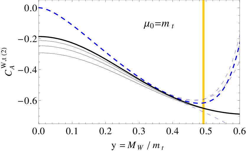 |
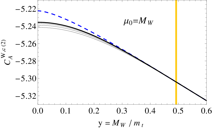
In Fig. 3, the results from Eqs. (26)–(29) are shown as functions of . The dashed and solid lines correspond to the and expansions, respectively. Thin lines are obtained by using less expansion terms in and . They can be used to test convergence of the expansions, as it is expected that good agreement with the unknown exact result is achieved up to the point where two successive orders almost coincide.
In the case of (left panel of Fig. 3), there is a significant overlap of the expansions around the two limits in the region from to . The agreement over such a large range arises probably due to the relatively simple dependence of on the top quark mass: only occurs through one-loop corrections to the gluon propagator. Note also that the numerical effect of the top quark mass is moderate: changes only by around 1.5% between the limit and the physical value of .
Also in the case of (right panel of Fig. 3) one observes an overlap of the expansions for and around . This feature allows us to use the expression in Eq. (28) for , and the one in Eq. (29) for . Due to the convergence properties (cf. thin lines) these expressions are excellent approximations to the exact result in the respective regions. In particular, for the physical region of , it is sufficient to use the expansion around .
For practical applications, it is useful to have short formulae which approximate near the physical value of . In the range , the fits
| (30) |
are accurate to better than 1% in the corresponding quantities.
3 -boson penguins

3.1 General remarks
The second type of contribution to arises from the so-called -boson penguins. Sample diagrams at the one-, two- and three-loop orders are shown in Fig. 4. In contrast to the -box diagrams, there is no contribution from evanescent operators to . However, flavour non-diagonal loop contributions to the light quark kinetic terms require introduction of an EW counterterm which already appears at the one-loop level. The corresponding counterterm Lagrangian (see Eq. (13) of Ref. [30]33 3 Flavour non-diagonal renormalization of the mass terms does not matter in the present calculation because we can treat the bottom quark as massless.) can be written in the following form
| (31) |
where is the covariant derivative involving the neutral gauge boson fields (, , ). While only the one-loop contributions to were needed in the case [29], now also the two- and three-loop corrections of order and matter. The two-loop ones were also necessary in Refs. [23, 24, 25, 26, 27]. Perturbative expansions of are conveniently written as
| (32) |

For determination of , a two-point function with incoming strange quark and outgoing bottom quark has to be considered. Sample diagrams at one, two and three loops are shown in Fig. 5. We refrain from explicitly listing the results but refer to [36] for computer-readable expressions.

The counterterm is either inserted in the tree-level amplitude or in two-loop diagrams containing a closed top quark loop on the gluon propagator, as shown in Fig. 6. Insertions of the counterterm into other loop contributions lead to massless tadpoles which vanish in dimensional regularization.
3.2 Fermion triangle contribution

There is a class of Feynman diagrams which require special attention, namely those containing a closed triangle quark loop (see Fig. 7). For these contributions, a naive treatment of as anticommuting is not possible, and a more careful investigation is necessary. We have followed two approaches which are described below. Similarly to the anomaly cancellation in the SM, contributions with the up, down, strange and charm quarks running in the triangle loop cancel pairwise within each family. Thus, only the top and bottom quarks need to be considered, as the top is the only massive quark in our calculation.
In our first approach, we adopt the prescription from Ref. [37] and replace the axial-vector coupling in the triangle loop as follows
| (33) |
In a next step, we pull out the tensor and take the trace of the loop diagram in dimensions. In the resulting object, we perform the replacements
| (34) |
and proceed from now on in the same way as with the other diagrams contributing to .
In the second approach, we do not take the trace in the triangle loop at all, but only use the cyclicity property for traces and anticommutation relations for the matrices (not for ) in order to put to the end of each product under the trace. Afterwards, we perform the tensor loop integration, and use again anticommutation relations to bring the resulting expressions to the form
| (35) |
where only the axial-vector part of the ( boson)-lepton coupling has been taken into account. In a next step, we add and subtract to the first, and to the second structure in Eq. (35). This way, we obtain the Wilson coefficients for the trace evanescent operators [38]
| (36) |
and a contribution to . Actually, the latter is given by times the prefactor of the second structure in Eq. (35).
The two methods, which lead to identical results for , have been applied both to the three-loop diagrams themselves and to the counterterm contributions (cf. Fig. 7).
3.3 Matching formula
In analogy to Eq. (12) we can write
| (37) |
where are the contributions from the triangle diagrams described in the previous subsection.
The calculation of proceeds along the same lines as for the -box contribution. In particular, we set all the external momenta to zero, and expand the Feynman integrals in the full theory both for and . Furthermore, we renormalize the top-quark mass, and the wave function in analogy to the -box case. As before, all loop corrections vanish in the effective theory, which finally leads to the following matching equation for ()
| (38) | |||||
with top-quark mass counterterms
| (39) |
denote tree-level contributions from the EW counterterm (31) which take a simple form
| (40) |
Finally, stands for the counterterm contributions from two-loop diagrams like those in Fig. 6.
We observe that after inserting explicit results on the right-hand side of Eq. (38), all the terms proportional to cancel out, and becomes independent of the weak mixing angle. This can be understood by recalling similarities between the boson and the photon couplings to other particles in the background field gauge, as well as the structure of the counterterm in Eq. (31). Once the quark kinetic terms in the effective theory are imposed to be flavour diagonal, the same must be true for dimension-four quark-photon couplings. In effect, the counterterm in Eq. (31) automatically renormalizes away all the zero-momentum quark-( boson) interactions that come with .
Another interesting thing to note is that at each loop order in the background field version of the ’t Hooft-Feynman gauge, which means that only the triangle contributions are non-vanishing in the charm sector. One of the ways to understand this fact is again by considering diagrams where the boson (together with the muons) is replaced by an external photon.
3.4 Results
With our calculation, we have confirmed the one- and two-loop results from Ref. [23] which are given by (for )
| (41) | |||||
Furthermore, similarly to , we obtain exact dependence on and for the -dependent terms which read
| (42) | |||||
For the generic three-loop contributions, terms up to order and have been evaluated, as in the -box case in Section 2. In a numerical form, they read
| (43) | |||||
For the fermion triangle contributions, all the contributions have cancelled out after matching. We find
| (44) | |||||
In the limit of large top quark mass, the coefficient grows as , which has its origin in the Yukawa interaction of the charged pseudo-goldstones with the top quark. For this reason, we plot in Fig. 8 the combination where sums of the results from Eqs. (43) and (44) are shown as dashed () and solid lines (). Note that after multiplication by , the latter is expanded in . Again, one observes that the two approximations coincide for , which suggests that a combination of the two expansions covers the whole range between and . In the physical region, the expansion around provides an excellent approximation. It is interesting to note that the fermion triangle contribution is more than an order of magnitude larger than . This is particularly true for the physical value of where we have .

A handy approximation formula which works to better than 1% for reads
| (45) |
4 Numerical analysis
In this section, we shall discuss numerical effects of our three-loop QCD corrections. The branching ratio in the SM is proportional to (cf. Eq. (6) with and ). Here, we shall consider only. Evaluation of the branching ratio itself is relegated to a parallel article [39] where also the new two-loop EW corrections [16] are included.
The relevant parameters are as follows. For the gauge boson masses, we take GeV [40] and GeV (calculated from , and ). For the strong coupling, in the five-flavour QCD is used [40]. Four-loop renormalization group equations (RGE) are applied to evolve it to other scales. For the top-quark mass, our input is GeV [40] which we treat as the pole mass. We convert it to the scheme with respect to QCD, but include no shift due to the EW interactions. This means that our should be understood as renormalized on-shell with respect to the EW interactions. As far as QCD is concerned, we use a three-loop relation for converting to , which gives GeV. Next, four-loop RGE are used to find at other values of .

Fig. 9 shows the matching scale dependence of . The dotted, dashed and solid curves show the leading order (LO), next-to-leading-order (NLO) and next-to-next-to-leading-order (NNLO) results, respectively. In the current case, they correspond to one-, two- and three-loop matching calculations.
The range of the plot corresponds roughly to , which might be considered reasonable given that both the -boson and the top quark are decoupled simultaneously. However, our Wilson coefficient has a trivial RGE (at the LO in EW interactions) but it is quite sensitive to . In consequence, the main reason for its -dependence here is the top-quark mass renormalization. Thus, for estimating uncertainties due to truncation of the QCD perturbation series at each order, we shall use a more narrow range .
One observes in Fig. 9 that the prediction for has already improved a lot after including the NLO QCD corrections. The variation at the NLO level amounts to around only, for . Once the new three-loop corrections are taken into account, the uncertainty gets reduced to less than , which can be treated as negligible for all practical purposes.
Another conclusion that can be drawn from Fig. 9 is that for the NLO correction is moderate (), while the NNLO correction essentially vanishes. Although has been anticipated to be an optimal scale in the past [24], there has been no convincing theoretical argument for such a choice. Our explicit three-loop calculation has been actually necessary to suppress the QCD matching uncertainties in to the current sub-percent level.
For GeV, our final result for is well approximated by the fit
| (46) |
which is accurate to better than for and GeV.
Let us stress that the term in Eq. (46) stands for both the NLO EW matching corrections at , as well as effects of the evolution of down to , according to the RGE. Once the QCD logarithms get resummed, the latter effects behave not only like , but also like and , which means that they are potentially more important than the NNLO QCD corrections evaluated here. However, the actual numerical impact of the and terms on the decay rate amounts to around only [41], which has been checked using anomalous dimension matrices from Refs. [42, 43]. The necessary expressions are given in the Appendix.
As far as the NLO EW matching corrections are concerned, they have been known for a long time only in the limit [44]. A complete calculation of these two-loop corrections has recently been finalized [16]. Their numerical effect depends on the scheme used at the LO. A detailed discussion of this issue is presented in Ref. [16]. Let us only mention that the semi-perfect stabilization of -dependence in Fig. 9 at the NNLO in QCD takes place only because we have renormalized and on shell with respect to the EW interactions. If we used at for the EW renormalization of and , then acceptable stability would be observed only after including the very two-loop EW corrections.
5 Conclusions
We have evaluated the NNLO QCD corrections to the Wilson coefficient that param-etrizes the branching ratio in the SM. For this purpose, three-loop matching between the SM and the relevant effective theory has been performed. Tadpole integrals depending on and have been evaluated with the help of expansions starting from the limits and , which for all practical purposes is equivalent to an exact calculation. When masses of the light quarks and their momenta are set to zero, care has to be taken about the so-called evanescent operators, similarly to the NLO case [25]. Such operators have also been helpful in dealing with diagrams where was present under traces.
Our results for the renormalized matching coefficients and can be downloaded in a computer-readable form from [36]. Including the new corrections makes more stable with respect to the matching scale at which the top-quark mass and are renormalized. Apart from , our calculation is directly applicable to all the decay modes, and it matters for other processes mediated by -penguins and -boxes, e.g., , , or short-distance contributions to . However, it is only for which the three-loop accuracy is relevant at present.
Acknowledgements
We thank Alexander Kurz for providing to us his FORM routine to compute tensor tadpole integrals to three loops. We are grateful to Christoph Bobeth, Martin Gorbahn and Emmanuel Stamou for helpful discussions and comments on the manuscript. This work was supported by the DFG through the SFB/TR 9 “Computational Particle Physics” and the Graduiertenkolleg “Elementarteilchenphysik bei höchster Energie und höchster Präzision”. M.M. acknowledges partial support by the National Science Centre (Poland) research project, decision DEC-2011/01/B/ST2/00438.
Appendix: Logarithmically enhanced QED corrections
In this appendix, we present explicit expressions for the logarithmically-enhanced QED corrections to . Beyond the LO in , its perturbative expansion at the matching scale reads
| (47) |
where stands for the scale-independent contribution as given in Eq. (9). Using the RGE from Refs. [42, 43] one obtains the following result at the scale
| (48) | |||||
where includes all the NLO EW corrections that are not logarithmically enhanced. The quantities depend on and . We find
| (49) |
with and the remaining coefficients summarized in Table 1. The functions , and originate from the one-loop SM matching conditions [22] for various operators in the effective theory. They read
| (50) |
The coefficients in Table 1 satisfy the following identities:
| (51) |
With the help of them one can easily check that the terms in Eq. (48) proportional to are finite in the limit . Logarithms with arise in this limit, which explains why the corresponding QED corrections are called logarithmically enhanced. The QED logarithms are not being resummed here. It is the resummation of QCD logarithms in the corresponding terms that brings inverse powers of into the final results.
References
- [1] R. Aaij et al. (LHCb Collaboration), Phys. Rev. Lett. 110 (2013) 021801 [arXiv:1211.2674].
- [2] R. Aaij et al. (LHCb Collaboration), Phys. Rev. Lett. 111, 101805 (2013) [arXiv:1307.5024].
- [3] S. Chatrchyan et al. (CMS Collaboration), Phys. Rev. Lett. 111, 101804 (2013) [arXiv:1307.5025].
- [4] CMS and LHCb Collaborations, conference report CMS-PAS-BPH-13-007, LHCb-CONF-2013-012, http://cds.cern.ch/record/1564324 .
- [5] V. M. Abazov et al. (D0 Collaboration), Phys. Lett. B 693 (2010) 539 [arXiv:1006.3469].
- [6] T. Aaltonen et al. (CDF Collaboration), Phys. Rev. Lett. 107 (2011) 191801 [arXiv:1107.2304].
- [7] S. Chatrchyan et al. (CMS Collaboration), JHEP 1204 (2012) 033 [arXiv:1203.3976].
- [8] R. Aaij et al. (LHCb Collaboration), Phys. Rev. Lett. 108 (2012) 231801 [arXiv:1203.4493].
- [9] G. Aad et al. (ATLAS Collaboration), Phys. Lett. B 713 (2012) 387 [arXiv:1204.0735].
- [10] P. Dimopoulos et al. (ETM Collaboration), JHEP 1201 (2012) 046 [arXiv:1107.1441].
- [11] C. McNeile, C. T. H. Davies, E. Follana, K. Hornbostel and G. P. Lepage (HPQCD Collaboration), Phys. Rev. D 85 (2012) 031503 [arXiv:1110.4510].
- [12] A. Bazavov et al. (Fermilab Lattice and MILC Collaborations), Phys. Rev. D 85 (2012) 114506 [arXiv:1112.3051].
- [13] F. Bernardoni et al., (ALPHA Collaboration), Nucl. Phys. Proc. Suppl. 234 (2013) 181 [arXiv:1210.6524].
- [14] N. Carrasco et al. (ETMC Collaboration), PoS ICHEP 2012 (2012) 428 [arXiv:1212.0301].
- [15] R. J. Dowdall et al. (HPQCD Collaboration), Phys. Rev. Lett. 110 (2013) 222003 [arXiv:1302.2644].
- [16] C. Bobeth, M. Gorbahn and E. Stamou, arXiv:1311.1348.
- [17] H. E. Logan and U. Nierste, Nucl. Phys. B 586 (2000) 39 [hep-ph/0004139].
- [18] C. Bobeth, A. J. Buras, F. Kruger and J. Urban, Nucl. Phys. B 630 (2002) 87 [hep-ph/0112305].
- [19] K. De Bruyn, R. Fleischer, R. Knegjens, P. Koppenburg, M. Merk and N. Tuning, Phys. Rev. D 86 (2012) 014027 [arXiv:1204.1735].
- [20] K. De Bruyn, R. Fleischer, R. Knegjens, P. Koppenburg, M. Merk, A. Pellegrino and N. Tuning, Phys. Rev. Lett. 109 (2012) 041801 [arXiv:1204.1737].
- [21] A. J. Buras, R. Fleischer, J. Girrbach and R. Knegjens, JHEP 1307 (2013) 77 [arXiv:1303.3820].
- [22] T. Inami and C. S. Lim, Prog. Theor. Phys. 65 (1981) 297 [Erratum-ibid. 65 (1981) 1772].
- [23] G. Buchalla and A. J. Buras, Nucl. Phys. B 398 (1993) 285.
- [24] G. Buchalla and A. J. Buras, Nucl. Phys. B 400 (1993) 225.
- [25] M. Misiak and J. Urban, Phys. Lett. B 451 (1999) 161 [hep-ph/9901278].
- [26] G. Buchalla and A. J. Buras, Nucl. Phys. B 548 (1999) 309 [hep-ph/9901288].
- [27] C. Bobeth, M. Misiak and J. Urban, Nucl. Phys. B 574 (2000) 291 [hep-ph/9910220].
- [28] J. Grigo, J. Hoff, P. Marquard and M. Steinhauser, Nucl. Phys. B 864 (2012) 580 [arXiv:1206.3418].
- [29] M. Misiak and M. Steinhauser, Nucl. Phys. B 683 (2004) 277 [hep-ph/0401041].
- [30] T. Hermann, M. Misiak and M. Steinhauser, JHEP 1211 (2012) 036 [arXiv:1208.2788].
- [31] P. Nogueira, J. Comp. Phys. 105 (1993) 279.
- [32]
T. Seidensticker,
hep-ph/9905298;
R. Harlander, T. Seidensticker and M. Steinhauser, Phys. Lett. B 426 (1998) 125 [hep-ph/9712228]. - [33] V. A. Smirnov, “Analytic tools for Feynman integrals,” Springer Tracts Mod. Phys. 250, 1 (2012).
- [34] M. Steinhauser, Comput. Phys. Commun. 134 (2001) 335 [hep-ph/0009029].
- [35] J.A.M. Vermaseren, Symbolic Manipulation with FORM, Computer Algebra Netherlands, Amsterdam, 1991.
- [36] http://www.ttp.kit.edu/Progdata/ttp13/ttp13-034
- [37] S. A. Larin, Phys. Lett. B 303 (1993) 113 [hep-ph/9302240].
- [38] M. Gorbahn and U. Haisch, Nucl. Phys. B 713 (2005) 291 [hep-ph/0411071].
- [39] C. Bobeth, M. Gorbahn, T. Hermann, M. Misiak, E. Stamou and M. Steinhauser, arXiv:1311.0903.
- [40] J. Beringer et al. (Particle Data Group Collaboration), Phys. Rev. D 86 (2012) 010001.
- [41] M. Misiak, “Rare B-Meson Decays,” in Proceedings of 15th Lomonosov Conference on Elementary Particle Physics (Moscow, Russia, August 18-24, 2011), p. 301, [arXiv:1112.5978].
- [42] C. Bobeth, P. Gambino, M. Gorbahn and U. Haisch, JHEP 0404 (2004) 071 [hep-ph/0312090].
- [43] T. Huber, E. Lunghi, M. Misiak and D. Wyler, Nucl. Phys. B 740 (2006) 105 [hep-ph/0512066].
- [44] G. Buchalla and A. J. Buras, Phys. Rev. D 57 (1998) 216 [hep-ph/9707243].