跳到论文正文
W Papers独立论文阅读器 arXiv:1311.1224 论文正文 计算阅读时间 · 0%
引用这篇论文根据当前论文元数据生成,正式投稿前建议核对。


License: arXiv.org perpetual non-exclusive license
arXiv:1311.1224v1 [math.NA] 05 Nov 2013

Time-splitting methods for the Westervelt equation \shortauthorlistB. Kaltenbacher, V. Nikolic, M. Thalhammer

Efficient time integration methods based on operator splitting and application to the Westervelt equation

Barbara Kaltenbacher
Alpen-Adria-Universität Klagenfurt
   Institut für Mathematik   
Universitätsstraße 65–67
   9020 Klagenfurt    Austria.
E-mail: Barbara.Kaltenbacher@uni-klu.ac.at
Vanja Nikolic
Alpen-Adria-Universität Klagenfurt
   Institut für Mathematik   
Universitätsstraße 65–67
   9020 Klagenfurt    Austria.
E-mail: Vanja.Nikolic@aau.at
Mechthild Thalhammer
Leopold–Franzens Universität Innsbruck
   Institut für Mathematik    Technikerstraße 13/VII    6020 Innsbruck    Austria.
E-mail: Mechthild.Thalhammer@uibk.ac.at
Abstract

Efficient time integration methods based on operator splitting are introduced for the Westervelt equation, a nonlinear damped wave equation that arises in nonlinear acoustics as mathematical model for the propagation of sound waves in high intensity ultrasound applications. For the first-order Lie–Trotter splitting method a global error estimate is deduced, confirming that the splitting method remains stable and that the nonstiff convergence order is retained in situations where the problem data are sufficiently regular. Fundamental ingredients in the stability and error analysis are regularity results for the Westervelt equation and related linear evolution equations of hyperbolic and parabolic type. Numerical examples illustrate and complement the theoretical investigations. Nonlinear evolution equations Westervelt equation Regularity of solutions Time-splitting methods Stability Local error expansion Convergence


1 Introduction

Scope of applications.

High intensity ultrasound plays a crucial role in numerous practical settings ranging from medical treatment like lithotripsy or thermotherapy to industrial applications like ultrasound cleaning or welding and sonochemistry; as a small selection, we mention the contributions [Dreyer et al.(2000), Kaltenbacher(2007)] and refer to the literature cited therein. Numerical simulation of high intensity ultrasound propagation is a valuable tool for the design and improvement of high intensity ultrasound devices but poses major challenges due to the nonlinearity of the underlying partial differential equations. Time integration methods for the equations of nonlinear acoustics have been investigated in [Dreyer et al.(2000), Kaltenbacher et al.(2002)]; however, the use of transient simulations within the mathematical optimisation of high intensity ultrasound devices still seems to be beyond the scope of these approaches. On the other hand, operator splitting methods have proven to be efficient time integration methods in the context of other classes of nonlinear partial differential equations, see for instance [Auzinger et al.(2013), Descombes and Thalhammer(2012)] and the references given therein. This motivates the investigation of time-splitting methods for the equations of nonlinear acoustics.

Westervelt equation.

In this work, we study time integration methods based on operator splitting for one of the classical models of nonlinear acoustics, the non-degenerate Westervelt equation

∂t​tψ⁡(x,t)−b​Δ​∂tψ⁡(x,t)−c2​Δ​ψ​(x,t)=βac2∂t(∂tψ(x,t))2,(x,t)∈Ω×(0,T]⊂ℝd×ℝ>0,\begin{split}&\partial_{tt}\psi(x,t)-b\,\Delta\,\partial_{t}\psi(x,t)-c^{2}\Delta\,\psi(x,t)\\ &\quad=\tfrac{\beta_{a}}{c^{2}}\,\partial_{t}\big(\partial_{t}\psi(x,t)\big)^{2}\,,\qquad(x,t)\in\Omega\times(0,T]\subset\mathbb{R}^{d}\times\mathbb{R}_{>0}\,,\end{split} (1.1a)
describing the propagation of the acoustic velocity potential ψ:Ω¯×[0,T]→ℝ\psi:\overline{\Omega}\times[0,T]\to\mathbb{R}, where c>0c>0 denotes the speed of sound, b>0b>0 the diffusivity of sound, and βa>1\beta_{a}>1 the parameter of nonlinearity; for details on the physical background as well as the derivation of the Westervelt equation we refer to the original work [Westervelt(1963)], see also [Kaltenbacher(2007)]. For our purposes, it is advantageous to employ a reformulation of (1.1a) as nonlinear evolutionary system
dd​t​u​(t)=F⁡(u⁡(t)),t∈(0,T],\tfrac{{\rm d}}{{\rm d}t}\,u(t)=F\big(u(t)\big)\,,\qquad t\in(0,T]\,, (1.1b)

for the abstract function u:[0,T]→X=X1×X2:t↦u⁡(t)=Ψ⁡(⋅,t)=(ψ⁡(⋅,t),∂tψ⁡(⋅,t))u:[0,T]\to X=X_{1}\times X_{2}:t\mapsto u(t)=\Psi(\cdot,t)=(\psi(\cdot,t),\partial_{t}\psi(\cdot,t)) with values in the underlying Banach space (X,∥⋅∥X)(X,\|\cdot\|_{X}).

Time-splitting methods.

Our main concern is to introduce and analyse operator splitting methods for the time integration of the non-degenerate Westervelt equation (1.1). Time-splitting methods for nonlinear evolution equations of the form (1.1b) utilise a natural decomposition of the defining operator

F=A+BF=A+B (1.2a)
and rely on the presumption that efficient numerical solvers are available for the associated subproblems
dd​t​v​(t)=A⁡(v⁡(t)),dd​t​w​(t)=B⁡(w⁡(t)),t∈(0,T].\tfrac{{\rm d}}{{\rm d}t}\,v(t)=A\big(v(t)\big)\,,\quad\tfrac{{\rm d}}{{\rm d}t}\,w(t)=B\big(w(t)\big)\,,\qquad t\in(0,T]\,. (1.2b)

We propose different decompositions for (1.1) which have in common that they require the numerical solution of a nonlinear diffusion equation in each time step.

Convergence analysis.

For the decomposition with the best performance in numerical tests we provide a detailed convergence analysis, adapting the approach exploited in [Descombes and Thalhammer(2012)] for the first-order Lie–Trotter splitting methods applied to nonlinear Schrödinger equations, see also [Auzinger et al.(2013)] for an extension to the second-order Strang splitting method. A rigorous stability and error analysis of time-splitting methods for the Westervelt equation (1.1) is a complex task; on the one hand, two unbounded nonlinear operators F=A+BF=A+B are present, contrary to nonlinear Schrödinger equations comprising a linear differential operator and a nonlinear multiplication operator, and, on the other hand, the underlying Banach space X=X1×X2X=X_{1}\times X_{2} is composed of two different function spaces reflecting the regularity of the solution components (ψ,∂tψ)(\psi,\partial_{t}\psi). As this considerably simplifies the local error analyis, we focus on the first-order Lie–Trotter splitting method, given by

u1=𝒮F​(h,u0)=ℰB​(h,ℰA​(h,u0))≈u⁡(h)=ℰF​(h,u⁡(0)),u_{1}=\mathscr{S}_{F}(h,u_{0})=\mathscr{E}_{B}\big(h,\mathscr{E}_{A}(h,u_{0})\big)\;\approx\;u(h)=\mathscr{E}_{F}\big(h,u(0)\big)\,,

and indicate the extension to higher-order splitting methods; here, we denote by ℰF,ℰA,ℰB\mathscr{E}_{F},\mathscr{E}_{A},\mathscr{E}_{B} the evolution operators associated with the Westervelt equation (1.1) and the subproblems (1.2). In situations where the problem data are sufficiently regular the obtained convergence result ensures that the Lie–Trotter splitting method remains stable and retains the nonstiff order of convergence. Fundamental ingredients in the stability and error analyis are regularity results for the Westervelt equation and related linear evolution equations of hyperbolic and parabolic type. Numerical examples illustrate and complement the theoretical investigations.

2 Westervelt equation

In this section, we introduce the initial-boundary value problem for the Westervelt equation and its abstract formulation as Cauchy problem. A regularity result, needed as a basic ingredient in the convergence analysis of time-splitting methods for the Westervelt equation, is deduced in Section 7.

Westervelt equation.

We study the following initial-boundary value problem for a function ψ:Ω¯×[0,T]⊂ℝd×ℝ≥0→ℝ:(x,t)↦ψ⁡(x,t)\psi:\overline{\Omega}\times[0,T]\subset\mathbb{R}^{d}\times\mathbb{R}_{\geq 0}\to\mathbb{R}:(x,t)\mapsto\psi(x,t)

{∂t​tψ⁡(x,t)−α​Δ​∂tψ⁡(x,t)−β​Δ​ψ​(x,t)=γ∂t(∂tψ(x,t))2=δ∂tψ(x,t)∂t​tψ(x,t),(x,t)∈Ω×(0,T],ψ⁡(x,t)​ given,(x,t)∈∂Ω×[0,T],ψ⁡(x,0)​ given,∂tψ⁡(x,0)​ given,x∈Ω,\begin{cases}&\partial_{tt}\psi(x,t)-\alpha\,\Delta\,\partial_{t}\psi(x,t)-\beta\,\Delta\,\psi(x,t)\\ &\quad=\gamma\,\partial_{t}\big(\partial_{t}\psi(x,t)\big)^{2}=\delta\,\partial_{t}\psi(x,t)\,\partial_{tt}\psi(x,t)\,,\quad(x,t)\in\Omega\times(0,T]\,,\\ &\psi(x,t)\;\text{ given}\,,\quad(x,t)\in\partial\Omega\times[0,T]\,,\\ &\psi(x,0)\;\text{ given}\,,\quad\partial_{t}\psi(x,0)\;\text{ given}\,,\quad x\in\Omega\,,\end{cases} (2.1a)
involving positive constants α,β,γ>0\alpha,\beta,\gamma>0 and δ=2​γ>0\delta=2\gamma>0. With regard to the time integration by first- and second-order splitting methods, we restrict ourselves to situations where a sufficiently regular solution to (2.1a) exists such that pointwise evaluations of the arising time and space derivatives of ψ\psi are justified; in particular, we suppose the spatial domain and the prescribed initial data to be sufficiently regular.
Reformulation (Non-degenerate case).

A regularity result for (2.1a), given in Section 7, ensures non-degeneracy of the Westervelt equation; that is, for any initial state of sufficiently small norm the relation 0<1−δ​∂tψ⁡(x,t)<∞0<1-\delta\,\partial_{t}\psi(x,t)<\infty holds for all (x,t)∈Ω¯×[0,T](x,t)\in\overline{\Omega}\times[0,T]. As a consequence, the equivalent formulation

{∂t​tψ⁡(x,t)=α​(1−δ​∂tψ⁡(x,t))−1​Δ​∂tψ⁡(x,t)+β​(1−δ​∂tψ⁡(x,t))−1​Δ​ψ​(x,t),(x,t)∈Ω×(0,T],ψ⁡(x,t)​ given,(x,t)∈∂Ω×[0,T],ψ⁡(x,0)​ given,∂tψ⁡(x,0)​ given,x∈Ω,\begin{cases}&\partial_{tt}\psi(x,t)=\alpha\,\big(1-\delta\,\partial_{t}\psi(x,t)\big)^{-1}\Delta\,\partial_{t}\psi(x,t)\\ &\qquad\qquad\qquad+\,\beta\,\big(1-\delta\,\partial_{t}\psi(x,t)\big)^{-1}\Delta\,\psi(x,t)\,,\quad(x,t)\in\Omega\times(0,T]\,,\\ &\psi(x,t)\;\text{ given}\,,\quad(x,t)\in\partial\Omega\times[0,T]\,,\\ &\psi(x,0)\;\text{ given}\,,\quad\partial_{t}\psi(x,0)\;\text{ given}\,,\quad x\in\Omega\,,\end{cases} (2.1b)

is obtained.

Reformulation as first-order system.

We next rewrite (2.1b) as a first-order system for the function Ψ=(Ψ1,Ψ2)=(ψ,∂tψ):Ω¯×[0,T]→ℝ2\Psi=(\Psi_{1},\Psi_{2})=(\psi,\partial_{t}\psi):\overline{\Omega}\times[0,T]\to\mathbb{R}^{2}

{∂tΨ1(x,t)=Ψ2(x,t),(x,t)∈Ω×(0,T],∂tΨ2​(x,t)=α​(1−δ​Ψ2​(x,t))−1​Δ​Ψ2​(x,t)OPEN+β​(1−δ​Ψ2​(x,t))−1​Δ​Ψ1​(x,t)),(x,t)∈Ω×(0,T],Ψ1​(x,t)​ given,(x,t)∈∂Ω×[0,T],Ψ1​(x,0)​ given,Ψ2​(x,0)​ given,x∈Ω.\begin{cases}&\partial_{t}\Psi_{1}(x,t)=\Psi_{2}(x,t)\,,\quad(x,t)\in\Omega\times(0,T]\,,\\ &\partial_{t}\Psi_{2}(x,t)=\alpha\,\big(1-\delta\,\Psi_{2}(x,t)\big)^{-1}\Delta\,\Psi_{2}(x,t)\\ &\qquad\qquad\qquad+\,\beta\,\big(1-\delta\,\Psi_{2}(x,t)\big)^{-1}\Delta\Psi_{1}(x,t)\big)\,,\quad(x,t)\in\Omega\times(0,T]\,,\\ &\Psi_{1}(x,t)\;\text{ given}\,,\quad(x,t)\in\partial\Omega\times[0,T]\,,\\ &\Psi_{1}(x,0)\;\text{ given}\,,\quad\Psi_{2}(x,0)\;\text{ given}\,,\quad x\in\Omega\,.\end{cases} (2.1c)
Abstract Cauchy problem.

In regard to the introduction and analysis of time-splitting methods for the Westervelt equation it is convenient to formulate (2.1) as abstract Cauchy problem for the function u:[0,T]→X:t↦u⁡(t)=Ψ⁡(⋅,t)u:[0,T]\to X:t\mapsto u(t)=\Psi(\cdot,t)

{dd​tu(t)=F(u(t)),t∈(0,T],u⁡(0)​ given,\begin{cases}&\tfrac{{\rm d}}{{\rm d}t}\,u(t)=F\big(u(t)\big)\,,\quad t\in(0,T]\,,\\ &u(0)\text{ given}\,,\end{cases} (2.2a)
where (X,∥⋅∥X)(X,\|\cdot\|_{X}) denotes the underlying Banach space and the nonlinear operator F:D⁡(F)→XF:D(F)\to X is given by
F(v)=(v2α~​(v2)​Δ​v2+β~​(v2)​Δ​v1),v=(v1,v2)∈D(F),α~(v2)=α(1−δv2)−1,β~(v2)=β(1−δv2)−1.\begin{gathered}F(v)=\begin{pmatrix}v_{2}\\ \widetilde{\alpha}(v_{2})\,\Delta v_{2}+\widetilde{\beta}(v_{2})\,\Delta v_{1}\end{pmatrix}\,,\qquad v=(v_{1},v_{2})\in D(F)\,,\\ \widetilde{\alpha}(v_{2})=\alpha\,\big(1-\delta v_{2}\big)^{-1}\,,\qquad\widetilde{\beta}(v_{2})=\beta\,\big(1-\delta v_{2}\big)^{-1}\,.\end{gathered} (2.2b)

According to the situation under consideration, the domain D⁡(F)⊂XD(F)\subset X is chosen such that it reflects the regularity requirements on the solution to the Westervelt equation as well as the imposed boundary conditions. It is notable that (2.2) can be cast into the form of a quasilinear problem, since

F⁡(v)=(0Iβ~​(v2)​Δα~​(v2)​Δ)​(v1v2),F(v)=\begin{pmatrix}0&\;I\\ \widetilde{\beta}(v_{2})\,\Delta&\;\;\widetilde{\alpha}(v_{2})\,\Delta\end{pmatrix}\begin{pmatrix}v_{1}\\ v_{2}\end{pmatrix}\,,

where II denotes the identity operator.

3 Time-splitting methods

In this section, we introduce the general format of exponential operator splitting methods for the time integration of nonlinear evolution equations and specify the different decompositions considered for the Westervelt equation. Numerical examples comparing the accuracy and efficiency of the resulting time dicretisations are found in Section 6.

3.1 Time-splitting methods for nonlinear evolution equations

Nonlinear evolution equation.

In accordance with the reformulation of the initial-boundary value problem for the Westervelt equation (2.1) as abstract Cauchy problem (2.2), we consider the initial value problem

{dd​tu(t)=F(u(t))=A(u(t))+B(u(t)),t∈(0,T],u⁡(0)​ given,\begin{cases}&\tfrac{{\rm d}}{{\rm d}t}\,u(t)=F\big(u(t)\big)=A\big(u(t)\big)+B\big(u(t)\big)\,,\quad t\in(0,T]\,,\\ &u(0)\text{ given}\,,\end{cases} (3.1a)
assuming that the nonlinear operators A:D⁡(A)→XA:D(A)\to X and B:D⁡(B)→XB:D(B)\to X are chosen such that the intersection D⁡(A)∩D⁡(B)D(A)\cap D(B) coincides with the domain of the defining operator F:D⁡(F)→XF:D(F)\to X. For the following investigations it is useful to introduce the evolution operator associated with (3.1a)
u⁡(t)=ℰF​(t,u⁡(0)),t∈[0,T].u(t)=\mathscr{E}_{F}\big(t,u(0)\big)\,,\qquad t\in[0,T]\,. (3.1b)
Subproblems.

Exponential operator splitting methods for the time integration of the initial value problem (3.1a) rely on the numerical solution of the subproblems

Subproblem A:{dd​tv(t)=A(v(t)),t∈(0,T],v⁡(0)​ given,Subproblem B:{dd​tw(t)=B(w(t)),t∈(0,T],w⁡(0)​ given.\begin{split}&\text{Subproblem A:}\qquad\begin{cases}&\tfrac{{\rm d}}{{\rm d}t}\,v(t)=A\big(v(t)\big)\,,\quad t\in(0,T]\,,\\ &v(0)\text{ given}\,,\end{cases}\\ &\text{Subproblem B:}\qquad\begin{cases}&\tfrac{{\rm d}}{{\rm d}t}\,w(t)=B\big(w(t)\big)\,,\quad t\in(0,T]\,,\\ &w(0)\text{ given}\,.\end{cases}\end{split} (3.2a)
In accordance with (3.1b) the associated evolution operators are given by
v⁡(t)=ℰA​(t,v⁡(0)),w⁡(t)=ℰB​(t,w⁡(0)),t∈[0,T].v(t)=\mathscr{E}_{A}\big(t,v(0)\big)\,,\quad w(t)=\mathscr{E}_{B}\big(t,w(0)\big)\,,\qquad t\in[0,T]\,. (3.2b)
Time-discrete solution.

For an initial approximation u0≈u⁡(0)u_{0}\approx u(0) and a sequence of time grid points 0=t0<t1<⋯<tN≤T0=t_{0}<t_{1}<\cdots<t_{N}\leq T with corresponding time stepsizes hn=tn+1−tnh_{n}=t_{n+1}-t_{n} for 0≤n≤N−10\leq n\leq N-1 the time-discrete solution to (3.1) is determined through a recurrence relation of the form

un=𝒮F​(hn−1,un−1)≈u⁡(tn)=ℰF​(hn−1,u⁡(tn−1)),1≤n≤N.u_{n}=\mathscr{S}_{F}(h_{n-1},u_{n-1})\;\approx\;u(t_{n})=\mathscr{E}_{F}\big(h_{n-1},u(t_{n-1})\big)\,,\qquad 1\leq n\leq N\,. (3.3a)
The numerical evolution operator associated with a general splitting method of (nonstiff) order p≥1p\geq 1 can be cast into the format
un=𝒮F​(hn−1,un−1)=Un−1,s,Un−1,j=ℰBj(hn−1,ℰAj(hn−1,Un−1,j−1)),1≤j≤s,Un−1,0=un−1,\begin{gathered}u_{n}=\mathscr{S}_{F}(h_{n-1},u_{n-1})=U_{n-1,s}\,,\\ U_{n-1,j}=\mathscr{E}_{B_{j}}\big(h_{n-1},\mathscr{E}_{A_{j}}(h_{n-1},U_{n-1,j-1})\big)\,,\quad 1\leq j\leq s\,,\quad U_{n-1,0}=u_{n-1}\,,\end{gathered} (3.3b)
involving certain coefficients (aj,bj)j=1s(a_{j},b_{j})_{j=1}^{s}. Here, we employ the abbreviations
Aj=aj​A,Bj=bj​B,1≤j≤s;A_{j}=a_{j}A\,,\quad B_{j}=b_{j}B\,,\qquad 1\leq j\leq s\,; (3.3c)

due to the fact that the considered evolution equation is autonomous, a scaling of the operators A,BA,B corresponds to a scaling in time.

Lie–Trotter and Strang splitting methods.

The Lie–Trotter splitting method of (nonstiff) order p=1p=1, given by

𝒮F​(t,v)=ℰB​(t,ℰA​(t,v))or𝒮F​(t,v)=ℰA​(t,ℰB​(t,v)),\mathscr{S}_{F}(t,v)=\mathscr{E}_{B}\big(t,\mathscr{E}_{A}(t,v)\big)\quad\text{or}\quad\mathscr{S}_{F}(t,v)=\mathscr{E}_{A}\big(t,\mathscr{E}_{B}(t,v)\big)\,, (3.4)

can be cast into the format (3.3) for the choices

s=1:a1=1,b1=1,ors=2:a1=0,b1=1,a2=1,b2=0,\begin{gathered}s=1:\qquad a_{1}=1\,,\quad b_{1}=1\,,\qquad\text{or}\\ s=2:\qquad a_{1}=0\,,\quad b_{1}=1\,,\quad a_{2}=1\,,\quad b_{2}=0\,,\end{gathered}

respectively. The widely used Strang splitting method of (nonstiff) order p=2p=2, given by

𝒮F​(t,v)=ℰ12​A​(t,ℰB​(t,ℰ12​A​(t,v)))or𝒮F​(t,v)=ℰ12​B​(t,ℰA​(t,ℰ12​B​(t,v)))\begin{gathered}\mathscr{S}_{F}(t,v)=\mathscr{E}_{\frac{1}{2}A}\big(t,\mathscr{E}_{B}\big(t,\mathscr{E}_{\frac{1}{2}A}(t,v)\big)\big)\quad\text{or}\\ \mathscr{S}_{F}(t,v)=\mathscr{E}_{\frac{1}{2}B}\big(t,\mathscr{E}_{A}\big(t,\mathscr{E}_{\frac{1}{2}B}(t,v)\big)\big)\end{gathered} (3.5)

results for the choices

s=2:a1=12,b1=1,a2=12,b2=0,ors=2:a1=0,b1=12,a2=1,b2=12,\begin{gathered}s=2:\qquad a_{1}=\tfrac{1}{2}\,,\quad b_{1}=1\,,\quad a_{2}=\tfrac{1}{2}\,,\quad b_{2}=0\,,\qquad\text{or}\\ s=2:\qquad a_{1}=0\,,\quad b_{1}=\tfrac{1}{2}\,,\quad a_{2}=1\,,\quad b_{2}=\tfrac{1}{2}\,,\end{gathered}

respectively.

3.2 Time-splitting methods for the Westervelt equation

In the following, we propose different decompositions

F=A+BF=A+B

of the nonlinear operator defining the Westervelt equation (2.1)–(2.2) and discuss the computational effort for the numerical solution of the associated subproblems (3.2).

3.2.1 Decomposition I

Decomposition.

A first decomposition involves the nonlinear operators

A(v)=(v2α~​(v2)​Δ​v2),B(v)=(0β~​(v2)​Δ​v1),α~(v2)=α(1−δv2)−1,β~(v2)=β(1−δv2)−1.\begin{gathered}A(v)=\begin{pmatrix}v_{2}\\ \widetilde{\alpha}(v_{2})\,\Delta v_{2}\end{pmatrix}\,,\qquad B(v)=\begin{pmatrix}0\\ \widetilde{\beta}(v_{2})\,\Delta v_{1}\end{pmatrix}\,,\\ \widetilde{\alpha}(v_{2})=\alpha\,\big(1-\delta v_{2}\big)^{-1}\,,\qquad\widetilde{\beta}(v_{2})=\beta\,\big(1-\delta v_{2}\big)^{-1}\,.\end{gathered}
Subproblems.

The resolution of the subproblem associated with AA

{∂tΨ1​(x,t)=Ψ2​(x,t),∂tΨ2​(x,t)=α​(1−δ​Ψ2​(x,t))−1​Δ​Ψ2​(x,t),\begin{cases}&\partial_{t}\Psi_{1}(x,t)=\Psi_{2}(x,t)\,,\\ &\partial_{t}\Psi_{2}(x,t)=\alpha\,\big(1-\delta\,\Psi_{2}(x,t)\big)^{-1}\Delta\Psi_{2}(x,t)\,,\end{cases}

amounts to the numerical solution of a nonlinear diffusion equation for the second component Ψ2=∂tψ\Psi_{2}=\partial_{t}\psi

∂tΨ2​(x,t)=α​(1−δ​Ψ2​(x,t))−1​Δ​Ψ2​(x,t);\partial_{t}\Psi_{2}(x,t)=\alpha\,\big(1-\delta\,\Psi_{2}(x,t)\big)^{-1}\Delta\Psi_{2}(x,t)\,;

the first component Ψ1=ψ\Psi_{1}=\psi is then retained by integration

Ψ1​(x,t)=Ψ1​(x,0)+∫0tΨ2​(x,τ)​𝑑τ.\Psi_{1}(x,t)=\Psi_{1}(x,0)+\int_{0}^{t}\Psi_{2}(x,\tau)\;{\rm d}\tau\,.

For the subproblem associated with BB

{∂tΨ1​(x,t)=0,∂tΨ2​(x,t)=β​(1−δ​Ψ2​(x,t))−1​Δ​Ψ1​(x,t),\begin{cases}&\partial_{t}\Psi_{1}(x,t)=0\,,\\ &\partial_{t}\Psi_{2}(x,t)=\beta\,\big(1-\delta\,\Psi_{2}(x,t)\big)^{-1}\Delta\Psi_{1}(x,t)\,,\end{cases}

the first component remains constant on the considered time interval

Ψ1​(x,t)=Ψ1​(x,0).\Psi_{1}(x,t)=\Psi_{1}(x,0)\,.

Consequently, the second component is a solution to

∂tΨ2​(x,t)=β​(1−δ​Ψ2​(x,t))−1​Δ​Ψ1​(x,0)\partial_{t}\Psi_{2}(x,t)=\beta\,\big(1-\delta\,\Psi_{2}(x,t)\big)^{-1}\Delta\Psi_{1}(x,0)

with explicit representation

Ψ2​(x,t)=1δ​(1−(1−δ​Ψ2​(x,0))2−2​β​δ​t​Δ​Ψ1​(x,0)).\Psi_{2}(x,t)=\tfrac{1}{\delta}\,\Big(1-\sqrt{\big(1-\delta\,\Psi_{2}(x,0)\big)^{2}-2\,\beta\delta\,t\,\Delta\Psi_{1}(x,0)}\;\Big)\,.

We note that in the non-degenerate case the relation δ​Ψ2​(x,0)<1\delta\,\Psi_{2}(x,0)<1 holds ; thus, the other admissable choice for a solution to the subproblem leads to a contradiction when evaluating at t=0t=0. Provided that the time increment t>0t>0 is chosen sufficiently small, it is ensured that (1−δ​Ψ2​(x,0))2−2​β​δ​t​Δ​Ψ1​(x,0)>0(1-\delta\,\Psi_{2}(x,0))^{2}-2\,\beta\delta\,t\,\Delta\Psi_{1}(x,0)>0 and hence Ψ2​(x,t)∈ℝ\Psi_{2}(x,t)\in\mathbb{R}.

3.2.2 Decomposition II

Decomposition.

A second decomposition involves the nonlinear operators

A⁡(v)=(12​v2α~​(v2)​Δ​v2),B⁡(v)=(12​v2β~​(v2)​Δ​v1).A(v)=\begin{pmatrix}\frac{1}{2}\,v_{2}\\ \widetilde{\alpha}(v_{2})\,\Delta v_{2}\end{pmatrix}\,,\qquad B(v)=\begin{pmatrix}\frac{1}{2}\,v_{2}\\ \widetilde{\beta}(v_{2})\,\Delta v_{1}\end{pmatrix}\,.
Subproblems.

The resolution of the subproblem associated with AA

{∂tΨ1​(x,t)=12​Ψ2​(x,t),∂tΨ2​(x,t)=α​(1−δ​Ψ2​(x,t))−1​Δ​Ψ2​(x,t),\begin{cases}&\partial_{t}\Psi_{1}(x,t)=\frac{1}{2}\,\Psi_{2}(x,t)\,,\\ &\partial_{t}\Psi_{2}(x,t)=\alpha\,\big(1-\delta\,\Psi_{2}(x,t)\big)^{-1}\Delta\Psi_{2}(x,t)\,,\end{cases}

requires the numerical solution of a nonlinear diffusion equation for the second component

∂tΨ2​(x,t)=α​(1−δ​Ψ2​(x,t))−1​Δ​Ψ2​(x,t);\partial_{t}\Psi_{2}(x,t)=\alpha\,\big(1-\delta\,\Psi_{2}(x,t)\big)^{-1}\Delta\Psi_{2}(x,t)\,;

the first component is then obtained by integration

Ψ1​(x,t)=Ψ1​(x,0)+12​∫0tΨ2​(x,τ)​𝑑τ.\Psi_{1}(x,t)=\Psi_{1}(x,0)+\tfrac{1}{2}\int_{0}^{t}\Psi_{2}(x,\tau)\;{\rm d}\tau\,.

The resolution of the subproblem associated with BB

{∂tΨ1​(x,t)=12​Ψ2​(x,t),∂tΨ2​(x,t)=β​(1−δ​Ψ2​(x,t))−1​Δ​Ψ1​(x,t),\begin{cases}&\partial_{t}\Psi_{1}(x,t)=\frac{1}{2}\,\Psi_{2}(x,t)\,,\\ &\partial_{t}\Psi_{2}(x,t)=\beta\,\big(1-\delta\,\Psi_{2}(x,t)\big)^{-1}\Delta\Psi_{1}(x,t)\,,\end{cases}

amounts to the numerical solution of a nonlinear wave equation for the first component

∂t​tΨ1​(t)=12​β​(1−2​δ​∂tΨ1​(x,t))−1​Δ​Ψ1​(x,t);\partial_{tt}\Psi_{1}(t)=\tfrac{1}{2}\,\beta\,\big(1-2\,\delta\,\partial_{t}\Psi_{1}(x,t)\big)^{-1}\Delta\Psi_{1}(x,t)\,;

the second component is then given by

Ψ2​(x,t)=2​∂tΨ1​(x,t).\Psi_{2}(x,t)=2\,\partial_{t}\Psi_{1}(x,t)\,.

3.2.3 Decomposition III

Decomposition.

A third decomposition involves the nonlinear operators

A⁡(v)=(0α~​(v2)​Δ​v2),B⁡(v)=(v2β~​(v2)​Δ​v1).A(v)=\begin{pmatrix}0\\ \widetilde{\alpha}(v_{2})\,\Delta v_{2}\end{pmatrix}\,,\qquad B(v)=\begin{pmatrix}v_{2}\\ \widetilde{\beta}(v_{2})\,\Delta v_{1}\end{pmatrix}\,.
Subproblems.

The resolution of the subproblem associated with AA

{∂tΨ1​(x,t)=0,∂tΨ2​(x,t)=α​(1−δ​Ψ2​(x,t))−1​Δ​Ψ2​(x,t),\begin{cases}&\partial_{t}\Psi_{1}(x,t)=0\,,\\ &\partial_{t}\Psi_{2}(x,t)=\alpha\,\big(1-\delta\,\Psi_{2}(x,t)\big)^{-1}\Delta\Psi_{2}(x,t)\,,\end{cases}

amounts to the numerical solution of a nonlinear diffusion equation for the second component

∂tΨ2​(x,t)=α​(1−δ​Ψ2​(x,t))−1​Δ​Ψ2​(x,t),\partial_{t}\Psi_{2}(x,t)=\alpha\,\big(1-\delta\,\Psi_{2}(x,t)\big)^{-1}\Delta\Psi_{2}(x,t)\,,

whereas the first component remains constant in time

Ψ1​(x,t)=Ψ1​(x,0).\Psi_{1}(x,t)=\Psi_{1}(x,0)\,.

The resolution of the subproblem associated with BB

{∂tΨ1​(x,t)=Ψ2​(x,t),∂tΨ2​(x,t)=β​(1−δ​Ψ2​(x,t))−1​Δ​Ψ1​(x,t),\begin{cases}&\partial_{t}\Psi_{1}(x,t)=\Psi_{2}(x,t)\,,\\ &\partial_{t}\Psi_{2}(x,t)=\beta\,\big(1-\delta\,\Psi_{2}(x,t)\big)^{-1}\Delta\Psi_{1}(x,t)\,,\end{cases}

requires the numerical solution of a nonlinear wave equation for the first component

∂t​tΨ1​(t)=β​(1−δ​∂tΨ1​(x,t))−1​Δ​Ψ1​(x,t);\partial_{tt}\Psi_{1}(t)=\beta\,\big(1-\delta\,\partial_{t}\Psi_{1}(x,t)\big)^{-1}\Delta\Psi_{1}(x,t)\,;

the second component is then given by

Ψ2​(x,t)=∂tΨ1​(x,t).\Psi_{2}(x,t)=\partial_{t}\Psi_{1}(x,t)\,.

3.2.4 Decomposition IV

Decomposition.

A fourth decomposition involves the nonlinear operators

A⁡(v)=(0α~​(v2)​Δ​v2+δ​v2​β~​(v2)​Δ​v1),B⁡(v)=(v2β​Δ​v1);A(v)=\begin{pmatrix}0\\ \widetilde{\alpha}(v_{2})\,\Delta v_{2}+\delta\,v_{2}\,\widetilde{\beta}(v_{2})\,\Delta v_{1}\end{pmatrix}\,,\qquad B(v)=\begin{pmatrix}v_{2}\\ \beta\,\Delta v_{1}\end{pmatrix}\,;

we note that the identity β+δ​v2​β~​(v2)=β~​(v2)\beta+\delta\,v_{2}\,\widetilde{\beta}(v_{2})=\widetilde{\beta}(v_{2}) holds.

Subproblems.

For the subproblem associated with AA

{∂tΨ1​(x,t)=0,∂tΨ2​(x,t)=α​(1−δ​Ψ2​(x,t))−1​Δ​Ψ2​(x,t)+β​δ​Ψ2​(x,t)​(1−δ​Ψ2​(x,t))−1​Δ​Ψ1​(x,t),\begin{cases}&\partial_{t}\Psi_{1}(x,t)=0\,,\\ &\partial_{t}\Psi_{2}(x,t)=\alpha\,\big(1-\delta\,\Psi_{2}(x,t)\big)^{-1}\Delta\Psi_{2}(x,t)\\ &\qquad\qquad\qquad+\;\beta\,\delta\,\Psi_{2}(x,t)\,\big(1-\delta\,\Psi_{2}(x,t)\big)^{-1}\Delta\Psi_{1}(x,t)\,,\end{cases}

the first component remains constant in time

Ψ1​(x,t)=Ψ1​(x,0),\Psi_{1}(x,t)=\Psi_{1}(x,0)\,,

whereas the computation of the second component requires the numerical solution of a nonlinear reaction-diffusion equation

∂tΨ2​(x,t)=α​(1−δ​Ψ2​(x,t))−1​Δ​Ψ2​(x,t)+β​δ​Ψ2​(x,t)​(1−δ​Ψ2​(x,t))−1​Δ​Ψ1​(x,0).\partial_{t}\Psi_{2}(x,t)=\alpha\,\big(1-\delta\,\Psi_{2}(x,t)\big)^{-1}\Delta\Psi_{2}(x,t)+\beta\,\delta\,\Psi_{2}(x,t)\,\big(1-\delta\,\Psi_{2}(x,t)\big)^{-1}\Delta\Psi_{1}(x,0)\,.

The resolution of the subproblem associated with BB

{∂tΨ1​(x,t)=Ψ2​(x,t),∂tΨ2​(x,t)=β​Δ​Ψ1​(x,t),\begin{cases}&\partial_{t}\Psi_{1}(x,t)=\Psi_{2}(x,t)\,,\\ &\partial_{t}\Psi_{2}(x,t)=\beta\,\Delta\Psi_{1}(x,t)\,,\end{cases}

amounts to the numerical solution of a linear wave equation for the first component

∂t​tΨ1​(x,t)=β​Δ​Ψ1​(x,t);\partial_{tt}\Psi_{1}(x,t)=\beta\,\Delta\Psi_{1}(x,t)\,;

the second component is then given by

Ψ2​(x,t)=∂tΨ1​(x,t).\Psi_{2}(x,t)=\partial_{t}\Psi_{1}(x,t)\,.

3.2.5 Computational effort

Subproblem A.

In all decompositions the realisation of the subproblem associated with the nonlinear operator AA requires the numerical solution of a nonlinear diffusion equation for the second component Ψ2=∂tψ\Psi_{2}=\partial_{t}\psi, where in case of Decomposition IV the nonlinear diffusion equation involves an additional zero-order term; the first component Ψ1=ψ\Psi_{1}=\psi is obtained by integration or remains constant in time.

Subproblem B.

In Decomposition I the realisation of the subproblem associated with the nonlinear operator BB reduces to the application of the Laplace operator to the first component of the imposed initial state; the second component is then computed through an explicit representation. Contrary, in Decomposition II-III the realisation of the subproblem amounts to the numerical solution of a nonlinear wave equation for the first component; the second component is then given by the time derivative ∂tΨ1\partial_{t}\Psi_{1}. We point out that the solvability of the arising nonlinear wave equations is an open question and that even local solvability in time cannot be guaranteed. As alternative we thus introduce Decomposition IV involving a linear wave equation.

4 Stability and error analysis

In this section, we describe the general approach for a convergence analysis of time-splitting methods, employing a framework of abstract Cauchy problems; details on the specialisation to the Westervelt equation are given in Section 5.

Uniform time grid.

For notational simplicity, we henceforth restrict ourselves to constant time increments h>0h>0 with associated equidistant time grid points given by tn=n​ht_{n}=nh for 0≤n≤N0\leq n\leq N. However, it is straightforward to extend the arguments to a non-uniform time grid with stepsize ratios bounded from above and below; in the global error estimate (4.2e) the constant time increment h>0h>0 is then replaced with the maximum stepsize hmax=max⁡{hn:0≤n≤N−1}h_{\max}=\max\{h_{n}:0\leq n\leq N-1\}.

Global and local error.

In order to deduce a convergence result for time-splitting methods (3.3) applied to nonlinear evolution equations (3.1), we utilise the telescopic identity

uN−u⁡(tN)=𝒮FN​(h,u0)−𝒮FN​(h,u⁡(0))+∑n=0N−1(𝒮FN−n−1(h,ℒF(h,u(tn))+ℰF(h,u(tn)))OPEN−𝒮FN−n−1​(h,ℰF​(h,u⁡(tn))))\begin{split}u_{N}-u(t_{N})&=\mathscr{S}_{F}^{N}\big(h,u_{0}\big)-\mathscr{S}_{F}^{N}\big(h,u(0)\big)\\ &\qquad+\sum_{n=0}^{N-1}\bigg(\mathscr{S}_{F}^{N-n-1}\Big(h,\mathscr{L}_{F}\big(h,u(t_{n})\big)+\mathscr{E}_{F}\big(h,u(t_{n})\big)\Big)\\ &\qquad\qquad\qquad-\mathscr{S}_{F}^{N-n-1}\Big(h,\mathscr{E}_{F}\big(h,u(t_{n})\big)\Big)\bigg)\end{split} (4.1a)
relating the global error to compositions of the splitting operator and local errors
𝒮Fn+1(h,v)=𝒮F(h,𝒮Fn(h,v)),0≤n≤N−1,𝒮F0(h,v)=v,ℒF(h,u(tn))=𝒮F(h,u(tn))−ℰF(h,u(tn)),0≤n≤N−1.\begin{gathered}\mathscr{S}_{F}^{n+1}(h,v)=\mathscr{S}_{F}\big(h,\mathscr{S}_{F}^{n}(h,v)\big)\,,\quad 0\leq n\leq N-1\,,\qquad\mathscr{S}_{F}^{0}(h,v)=v\,,\\ \mathscr{L}_{F}\big(h,u(t_{n})\big)=\mathscr{S}_{F}\big(h,u(t_{n})\big)-\mathscr{E}_{F}\big(h,u(t_{n})\big)\,,\quad 0\leq n\leq N-1\,.\end{gathered} (4.1b)
Approach.

Our aim is to deduce an estimate for the global error (4.1) with respect to the norm of the underlying Banach space XX or a suitable subspace X~⊂X\widetilde{X}\subset X, respectively, such that the expected dependence on the time stepsize is retained under appropriate regularity requirements on the problem data. In the context of the Westervelt equation, we shall make use of the fact that the regularity result stated in Section 7 implies

u(0)∈D,∥u(0)∥D≤C0⟹u(t)∈D,∥u(t)∥D≤C,t∈[0,T],u(0)\in D\,,\;\big\|u(0)\big\|_{D}\leq C_{0}\quad\Longrightarrow\quad u(t)\in D\,,\;\big\|u(t)\big\|_{D}\leq C\,,\quad t\in[0,T]\,, (4.2a)
for certain constants C0,C>0C_{0},C>0; the subspace D⊂X~⊂XD\subset\widetilde{X}\subset X, chosen accordingly to the (nonstiff) order of the splitting method, captures additional regularity and compatibility requirements. Regularity results for the arising subproblems and associated variational equations shall ensure stability of the splitting procedure, that is, boundedness of compositions of the splitting operator
‖𝒮Fn​(h,v)−𝒮Fn​(h,v~)‖X~≤eC​tn​‖v−v~‖X~,1≤n≤N,\big\|\mathscr{S}_{F}^{n}(h,v)-\mathscr{S}_{F}^{n}(h,\widetilde{v})\big\|_{\widetilde{X}}\leq{\rm e}^{Ct_{n}}\big\|v-\widetilde{v}\big\|_{\widetilde{X}}\,,\qquad 1\leq n\leq N\,, (4.2b)
provided that the arguments v,v~∈D~v,\widetilde{v}\in\widetilde{D} remain bounded in a certain subspace D⊂D~⊂X~⊂XD\subset\widetilde{D}\subset\widetilde{X}\subset X. Concerning a local error analysis, we restrict ourselves to the least technical case, the first-order Lie–Trotter splitting method given by
𝒮F​(h,v)=ℰB​(h,ℰA​(h,v)),\mathscr{S}_{F}(h,v)=\mathscr{E}_{B}\big(h,\mathscr{E}_{A}(h,v)\big)\,,
see also (3.4); here, a suitable expansion yields the representation
ℒF​(h,v)=∫0h∫0τ1∂2ℰF​(h−τ1,𝒮F​(τ1,v))​∂2ℰB​(τ1,w)​(∂2ℰB​(τ2,w))−1×[B,A]​(ℰB​(τ2,w))|w=ℰA​(τ1,v)​d​τ2​d​τ1,\begin{split}\mathscr{L}_{F}(h,v)&=\int_{0}^{h}\int_{0}^{\tau_{1}}\partial_{2}\mathscr{E}_{F}\big(h-\tau_{1},\mathscr{S}_{F}(\tau_{1},v)\big)\,\partial_{2}\mathscr{E}_{B}(\tau_{1},w)\,\big(\partial_{2}\mathscr{E}_{B}(\tau_{2},w)\big)^{-1}\\ &\qquad\qquad\quad\times\big[B,A\big]\big(\mathscr{E}_{B}(\tau_{2},w)\big)\Big|_{w=\mathscr{E}_{A}(\tau_{1},v)}\;{\rm d}\tau_{2}\,{\rm d}\tau_{1}\,,\end{split} (4.2c)
see [Auzinger et al.(2013), Descombes and Thalhammer(2012)] and formula (A.12) in Section A. Bounds for the evolution operators ℰF,ℰA,ℰB\mathscr{E}_{F},\mathscr{E}_{A},\mathscr{E}_{B}, their Fréchet derivatives with respect to the second argument ∂2ℰF,∂2ℰA,∂2ℰB\partial_{2}\mathscr{E}_{F},\partial_{2}\mathscr{E}_{A},\partial_{2}\mathscr{E}_{B}, and the first Lie-commutator [A,B][A,B] shall lead to the local error estimate
p=1:‖ℒF​(h,v)‖X~≤C​hp+1.p=1:\qquad\big\|\mathscr{L}_{F}(h,v)\big\|_{\widetilde{X}}\leq C\,h^{p+1}\,. (4.2d)
Altogether, these ingredients allow to establish the global error estimate
‖uN−u⁡(tN)‖X~≤‖𝒮FN​(h,u0)−𝒮FN​(h,u⁡(0))‖X~+∑n=0N−1∥𝒮FN−n−1(h,ℒF(h,u(tn))+ℰF(h,u(tn)))−𝒮FN−n−1(h,ℰF(h,u(tn)))∥X~≤C⁡(‖u0−u⁡(0)‖X~+∑n=1N‖ℒF​(h,u⁡(tn−1))‖X~)≤C⁡(‖u0−u⁡(0)‖X~+hp)\begin{split}\big\|u_{N}-u(t_{N})\big\|_{\widetilde{X}}&\leq\big\|\mathscr{S}_{F}^{N}\big(h,u_{0}\big)-\mathscr{S}_{F}^{N}\big(h,u(0)\big)\big\|_{\widetilde{X}}\\ &\qquad+\sum_{n=0}^{N-1}\Big\|\mathscr{S}_{F}^{N-n-1}\Big(h,\mathscr{L}_{F}\big(h,u(t_{n})\big)+\mathscr{E}_{F}\big(h,u(t_{n})\big)\Big)\\ &\qquad\qquad\qquad-\mathscr{S}_{F}^{N-n-1}\Big(h,\mathscr{E}_{F}\big(h,u(t_{n})\big)\Big)\Big\|_{\widetilde{X}}\\ &\leq C\,\bigg(\big\|u_{0}-u(0)\big\|_{\widetilde{X}}+\sum_{n=1}^{N}\big\|\mathscr{L}_{F}\big(h,u(t_{n-1})\big)\big\|_{\widetilde{X}}\bigg)\\ &\leq C\,\Big(\big\|u_{0}-u(0)\big\|_{\widetilde{X}}+h^{p}\Big)\end{split} (4.2e)

with constant depending in particular on the bound for the exact solution values with respect to the norm in DD, the bound for the initial approximation u0u_{0} in D~\widetilde{D}, and the final time; this shows that the nonstiff order of concergence is retained, provided that the prescribed initial state is sufficiently regular.

5 Global error estimate

In this section, we establish a global error estimate for the Lie–Trotter splitting method applied to the Westervelt equation. We include a detailed stability and error analysis for Decomposition I showing the best performance in numerical tests, see Section 3.2 . In accordance with Section 7 we study the Westervelt equation in three space dimensions subject to homogeneous Dirichlet boundary conditions on a regular domain; we consider this to be the least technical case, as far as the boundary conditions are concerned, and the most relevant case, as far as the space dimension is concerned. Fundamental auxiliary results for the proof of Theorem 5.1 are deduced in Sections 5.1–5.2.

5.1 Fréchet derivative and Lie-commutator

In the following, we specify the Fréchet derivative of the operator defining (2.1)–(2.2) and determine the first Lie-commutator arising in the local error representation (4.2c).

Notation and auxiliary estimates.

The product space X=X1×X2X=X_{1}\times X_{2} of two Banach spaces is endowed with the norm ‖(x1,x2)‖X=‖x1‖X1+‖x2‖X2\|(x_{1},x_{2})\|_{X}=\|x_{1}\|_{X_{1}}+\|x_{2}\|_{X_{2}}. We employ standard abbreviations for Sobolev spaces such as (Wk,p(Ω),∥⋅∥Wk,p)(W^{k,p}(\Omega),\|\cdot\|_{W^{k,p}}) and Hk​(Ω)=Wk,2​(Ω)H^{k}(\Omega)=W^{k,2}(\Omega) for k∈ℕ≥0k\in\mathbb{N}_{\geq 0} and p∈ℕ≥1p\in\mathbb{N}_{\geq 1}, see for instance [Adams and Fournier(2003)]; for notational simplicity, in the norms we do not indicate the dependence on the domain. For convenience, we recall Young’s inequality

a​b≤app+bqq,a,b≥0,1<p,q<∞,1p+1q=1.ab\leq\tfrac{a^{p}}{p}+\tfrac{b^{q}}{q}\,,\qquad a,b\geq 0\,,\quad 1<p,q<\infty\,,\quad\tfrac{1}{p}+\tfrac{1}{q}=1\,. (5.1a)
By means of Hölder’s inequality
‖f1​f2‖L1≤‖f1‖Lp​‖f2‖Lq,1≤p,q≤∞,1p+1q=1,\big\|f_{1}\,f_{2}\big\|_{L^{1}}\leq\big\|f_{1}\big\|_{L^{p}}\,\big\|f_{2}\big\|_{L^{q}}\,,\qquad 1\leq p,q\leq\infty\,,\quad\tfrac{1}{p}+\tfrac{1}{q}=1\,, (5.1b)
and the continuous embeddings H2​(Ω)↪𝒞⁡(Ω)H^{2}(\Omega)\hookrightarrow\mathscr{C}(\Omega) as well as H1​(Ω)↪L4​(Ω),L6​(Ω)H^{1}(\Omega)\hookrightarrow L^{4}(\Omega),L^{6}(\Omega), valid for any bounded regular domain Ω⊂ℝ3\Omega\subset\mathbb{R}^{3}, the relations
‖f1​f2‖L2≤‖f1‖L∞​‖f2‖L2≤C​‖f1‖H2​‖f2‖L2,‖f1​f2‖L2≤‖f1‖L4​‖f2‖L4≤C​‖f1‖H1​‖f2‖H1,‖f1​f2‖L2≤‖f1‖L3​‖f2‖L6≤C​‖f1‖H1​‖f2‖H1,‖f1​f2​f3‖L2≤‖f1‖L6​‖f2‖L6​‖f3‖L6≤C​‖f1‖H1​‖f2‖H1​‖f3‖H1,\begin{gathered}\big\|f_{1}\,f_{2}\big\|_{L^{2}}\leq\big\|f_{1}\big\|_{L^{\infty}}\big\|f_{2}\big\|_{L^{2}}\leq C\,\big\|f_{1}\big\|_{H^{2}}\big\|f_{2}\big\|_{L^{2}}\,,\\ \big\|f_{1}\,f_{2}\big\|_{L^{2}}\leq\big\|f_{1}\big\|_{L^{4}}\big\|f_{2}\big\|_{L^{4}}\leq C\,\big\|f_{1}\big\|_{H^{1}}\big\|f_{2}\big\|_{H^{1}}\,,\\ \big\|f_{1}\,f_{2}\big\|_{L^{2}}\leq\big\|f_{1}\big\|_{L^{3}}\big\|f_{2}\big\|_{L^{6}}\leq C\,\big\|f_{1}\big\|_{H^{1}}\big\|f_{2}\big\|_{H^{1}}\,,\\ \big\|f_{1}\,f_{2}\,f_{3}\big\|_{L^{2}}\leq\big\|f_{1}\big\|_{L^{6}}\big\|f_{2}\big\|_{L^{6}}\big\|f_{3}\big\|_{L^{6}}\leq C\,\big\|f_{1}\big\|_{H^{1}}\big\|f_{2}\big\|_{H^{1}}\big\|f_{3}\big\|_{H^{1}}\,,\end{gathered} (5.1c)
follow. Moreover, we make use of the fact that Hk+2​(Ω)H^{k+2}(\Omega) forms an algebra for arbitrary exponents k∈ℕ≥0k\in\mathbb{N}_{\geq 0}, that is, the relation
‖f1​f2‖Hk+2≤C​‖f1‖Hk+2​‖f2‖Hk+2,k∈ℕ≥0,\big\|f_{1}\,f_{2}\big\|_{H^{k+2}}\leq C\,\|f_{1}\|_{H^{k+2}}\,\|f_{2}\|_{H^{k+2}}\,,\qquad k\in\mathbb{N}_{\geq 0}\,, (5.1d)
holds. This in particular implies
‖∇f1⋅∇f2‖Hk+2≤C​‖f1‖Hk+3​‖f2‖Hk+3,k∈ℕ≥0.\big\|\nabla f_{1}\cdot\nabla f_{2}\big\|_{H^{k+2}}\leq C\,\|f_{1}\|_{H^{k+3}}\,\|f_{2}\|_{H^{k+3}}\,,\qquad k\in\mathbb{N}_{\geq 0}\,. (5.1e)
Defining operators.

For the convenience of the reader, we recall the definitions of the nonlinear operators associated with Decomposition I

F⁡(v)=A⁡(v)+B⁡(v),A(v)=(v2α~​(v2)​Δ​v2),B(v)=(0β~​(v2)​Δ​v1),α~(v2)=α(1−δv2)−1,β~(v2)=β(1−δv2)−1.\begin{gathered}F(v)=A(v)+B(v)\,,\\ A(v)=\begin{pmatrix}v_{2}\\ \widetilde{\alpha}(v_{2})\,\Delta v_{2}\end{pmatrix}\,,\qquad B(v)=\begin{pmatrix}0\\ \widetilde{\beta}(v_{2})\,\Delta v_{1}\end{pmatrix}\,,\\ \widetilde{\alpha}(v_{2})=\alpha\,\big(1-\delta v_{2}\big)^{-1}\,,\qquad\widetilde{\beta}(v_{2})=\beta\,\big(1-\delta v_{2}\big)^{-1}\,.\end{gathered}

Under the non-degeneracy condition 0<ν¯≤1−δ​v2​(x)≤ν¯<∞0<\underline{\nu}\leq 1-\delta\,v_{2}(x)\leq\overline{\nu}<\infty for all x∈Ω¯x\in\overline{\Omega}, justified by Theorem 7.1 in Section 7, the auxiliary results in (5.1) imply

‖α~​(v2)‖Hk+2+‖β~​(v2)‖Hk+2≤C⁡(‖v2‖Hk+2),k∈ℕ≥0,\big\|\widetilde{\alpha}(v_{2})\big\|_{H^{k+2}}+\big\|\widetilde{\beta}(v_{2})\big\|_{H^{k+2}}\leq C\big(\|v_{2}\|_{H^{k+2}}\big)\,,\qquad k\in\mathbb{N}_{\geq 0}\,,

and further lead to the estimates

‖α~​(v2)​Δ​v2‖L2≤C⁡(‖v2‖H2),‖β~​(v2)​Δ​v1‖L2≤C⁡(‖v1‖H2,‖v2‖H2),∥α~(v2)Δv2∥Hk+2≤C(∥v2∥Hk+4),k∈ℕ≥0,∥β~(v2)Δv1∥Hk+2≤C(∥v1∥Hk+4,∥v2∥Hk+2),k∈ℕ≥0,\begin{gathered}\big\|\widetilde{\alpha}(v_{2})\,\Delta v_{2}\big\|_{L^{2}}\leq C\big(\|v_{2}\|_{H^{2}}\big)\,,\\ \big\|\widetilde{\beta}(v_{2})\,\Delta v_{1}\big\|_{L^{2}}\leq C\big(\|v_{1}\|_{H^{2}},\|v_{2}\|_{H^{2}}\big)\,,\\ \big\|\widetilde{\alpha}(v_{2})\,\Delta v_{2}\big\|_{H^{k+2}}\leq C\big(\|v_{2}\|_{H^{k+4}}\big)\,,\qquad k\in\mathbb{N}_{\geq 0}\,,\\ \big\|\widetilde{\beta}(v_{2})\,\Delta v_{1}\big\|_{H^{k+2}}\leq C\big(\|v_{1}\|_{H^{k+4}},\|v_{2}\|_{H^{k+2}}\big)\,,\qquad k\in\mathbb{N}_{\geq 0}\,,\end{gathered}

with constants C⁡(⋅)C(\cdot) depending on bounds for the arising norms of the solution components v1,v2v_{1},v_{2}.

Fréchet derivatives.

The Fréchet derivatives of the nonlinear operators associated with Decomposition I are given by

F′​(v)=A′​(v)+B′​(v),A′(v)=(0I0α~​(v2)​Δ+α~′​(v2)​Δ​v2),B′(v)=(0 0β~​(v2)​Δβ~′​(v2)​Δ​v1),α~′(v2)=αδ(1−δv2)−2=δα(α~(v2))2,β~′(v2)=βδ(1−δv2)−2=δβ(β~(v2))2;\begin{gathered}F^{\prime}(v)=A^{\prime}(v)+B^{\prime}(v)\,,\\ A^{\prime}(v)=\begin{pmatrix}0&\;I\\ 0&\;\widetilde{\alpha}(v_{2})\,\Delta+\widetilde{\alpha}^{\prime}(v_{2})\,\Delta v_{2}\end{pmatrix}\,,\qquad B^{\prime}(v)=\begin{pmatrix}0&\;0\\ \widetilde{\beta}(v_{2})\,\Delta&\;\widetilde{\beta}^{\prime}(v_{2})\,\Delta v_{1}\end{pmatrix}\,,\\ \widetilde{\alpha}^{\prime}(v_{2})=\alpha\,\delta\,\big(1-\delta v_{2}\big)^{-2}=\tfrac{\delta}{\alpha}\,\big(\widetilde{\alpha}(v_{2})\big)^{2}\,,\qquad\widetilde{\beta}^{\prime}(v_{2})=\beta\,\delta\,\big(1-\delta v_{2}\big)^{-2}=\tfrac{\delta}{\beta}\,\big(\widetilde{\beta}(v_{2})\big)^{2}\,;\end{gathered}

more precisely, application to an element w=(w1,w2)w=(w_{1},w_{2}) yields

A′​(v)​w=(w2α~​(v2)​Δ​w2+α~′​(v2)​Δ​v2​w2),B′​(v)​w=(0β~​(v2)​Δ​w1+β~′​(v2)​Δ​v1​w2).\begin{gathered}A^{\prime}(v)\,w=\begin{pmatrix}w_{2}\\ \widetilde{\alpha}(v_{2})\,\Delta w_{2}+\widetilde{\alpha}^{\prime}(v_{2})\,\Delta v_{2}\,w_{2}\end{pmatrix}\,,\\ B^{\prime}(v)\,w=\begin{pmatrix}0\\ \widetilde{\beta}(v_{2})\,\Delta w_{1}+\widetilde{\beta}^{\prime}(v_{2})\,\Delta v_{1}\,w_{2}\end{pmatrix}\,.\end{gathered}
Lie-commutator.

In order to determine the first Lie-commutator

[A,B]​(v)=A′​(v)​B​(v)−B′​(v)​A​(v),\big[A,B\big](v)=A^{\prime}(v)\,B(v)-B^{\prime}(v)\,A(v)\,,

see also (A.6), we employ the auxiliary relations

∇β~(v2)=β~′(v2)∇v2,Δβ~(v2)=β~′′(v2)∇v2⋅∇v2+β~′(v2)Δv2,Δ(β~(v2)Δv1)=Δβ~(v2)Δv1+2∇β~(v2)⋅∇Δv1+β~(v2)Δ2v1,β~′′​(v2)=2​β​δ2​(1−δ​v2)−3=2​(δβ)2​(β~​(v2))3.\begin{gathered}\nabla\widetilde{\beta}(v_{2})=\widetilde{\beta}^{\prime}(v_{2})\,\nabla v_{2}\,,\\ \Delta\,\widetilde{\beta}(v_{2})=\widetilde{\beta}^{\prime\prime}(v_{2})\,\nabla v_{2}\cdot\nabla v_{2}+\widetilde{\beta}^{\prime}(v_{2})\,\Delta v_{2}\,,\\ \Delta\,\big(\widetilde{\beta}(v_{2})\,\Delta v_{1}\big)=\Delta\,\widetilde{\beta}(v_{2})\,\Delta v_{1}+2\,\nabla\widetilde{\beta}(v_{2})\cdot\nabla\Delta v_{1}+\widetilde{\beta}(v_{2})\,\Delta^{2}v_{1}\,,\\ \widetilde{\beta}^{\prime\prime}(v_{2})=2\,\beta\,\delta^{2}\big(1-\delta v_{2}\big)^{-3}=2\,\big(\tfrac{\delta}{\beta}\big)^{2}\,\big(\widetilde{\beta}(v_{2})\big)^{3}\,.\end{gathered}

Noting that the identity α~′​(v2)​β~​(v2)−α~​(v2)​β~′​(v2)=0\widetilde{\alpha}^{\prime}(v_{2})\,\widetilde{\beta}(v_{2})-\widetilde{\alpha}(v_{2})\,\widetilde{\beta}^{\prime}(v_{2})=0 holds, a brief calculation yields

[A,B]​(v)=(0I0α~′​(v2)​Δ​v2+α~​(v2)​Δ)​(0β~​(v2)​Δ​v1)−(0 0β~​(v2)​Δβ~′​(v2)​Δ​v1)​(v2α~​(v2)​Δ​v2)=(β~​(v2)​Δ​v1(α~′​(v2)​β~​(v2)−α~​(v2)​β~′​(v2))​Δ​v1​Δ​v2+α~​(v2)​Δ​(β~​(v2)​Δ​v1)−β~​(v2)​Δ​v2)=(β~​(v2)​Δ​v1α~​(v2)​Δ​(β~​(v2)​Δ​v1)−β~​(v2)​Δ​v2)=(β~​(v2)​Δ​v1α~(v2)(Δβ~(v2)Δv1+2∇β~(v2)⋅∇Δv1+β~(v2)Δ2v1)−β~(v2)Δv2),\begin{split}&\big[A,B\big](v)\\ &\;\;=\begin{pmatrix}0&\;I\\ 0&\;\widetilde{\alpha}^{\prime}(v_{2})\,\Delta v_{2}+\widetilde{\alpha}(v_{2})\,\Delta\end{pmatrix}\,\begin{pmatrix}0\\ \widetilde{\beta}(v_{2})\,\Delta v_{1}\end{pmatrix}-\begin{pmatrix}0&\;0\\ \widetilde{\beta}(v_{2})\,\Delta&\;\widetilde{\beta}^{\prime}(v_{2})\,\Delta v_{1}\end{pmatrix}\begin{pmatrix}v_{2}\\ \widetilde{\alpha}(v_{2})\,\Delta v_{2}\end{pmatrix}\\ &\;\;=\begin{pmatrix}\widetilde{\beta}(v_{2})\,\Delta v_{1}\\ \big(\widetilde{\alpha}^{\prime}(v_{2})\,\widetilde{\beta}(v_{2})-\widetilde{\alpha}(v_{2})\,\widetilde{\beta}^{\prime}(v_{2})\big)\,\Delta v_{1}\,\Delta v_{2}+\widetilde{\alpha}(v_{2})\,\Delta\,\big(\widetilde{\beta}(v_{2})\,\Delta v_{1}\big)-\widetilde{\beta}(v_{2})\,\Delta v_{2}\end{pmatrix}\\ &\;\;=\begin{pmatrix}\widetilde{\beta}(v_{2})\,\Delta v_{1}\\ \widetilde{\alpha}(v_{2})\,\Delta\,\big(\widetilde{\beta}(v_{2})\,\Delta v_{1}\big)-\widetilde{\beta}(v_{2})\,\Delta v_{2}\end{pmatrix}\\ &\;\;=\begin{pmatrix}\widetilde{\beta}(v_{2})\,\Delta v_{1}\\ \widetilde{\alpha}(v_{2})\,\big(\Delta\,\widetilde{\beta}(v_{2})\,\Delta v_{1}+2\,\nabla\widetilde{\beta}(v_{2})\cdot\nabla\Delta v_{1}+\widetilde{\beta}(v_{2})\,\Delta^{2}v_{1}\big)-\widetilde{\beta}(v_{2})\,\Delta v_{2}\end{pmatrix}\,,\end{split}

that is, we have

[A,B](v)=(ζ1ζ2),ζ1=β~(v2)Δv1,ζ2=α~(v2)(Δβ~(v2)Δv1+2∇β~(v2)⋅∇Δv1+β~(v2)Δ2v1)−β~(v2)Δv2.\begin{gathered}\big[A,B\big](v)=\begin{pmatrix}\zeta_{1}\\ \zeta_{2}\end{pmatrix}\,,\qquad\zeta_{1}=\widetilde{\beta}(v_{2})\,\Delta v_{1}\,,\\ \zeta_{2}=\widetilde{\alpha}(v_{2})\,\big(\Delta\,\widetilde{\beta}(v_{2})\,\Delta v_{1}+2\,\nabla\widetilde{\beta}(v_{2})\cdot\nabla\Delta v_{1}+\widetilde{\beta}(v_{2})\,\Delta^{2}v_{1}\big)-\widetilde{\beta}(v_{2})\,\Delta v_{2}\,.\end{gathered}

As a consequence, by means of the relations

‖ζ1‖L2≤C⁡(‖v1‖H2,‖v2‖H2),‖ζ2‖L2≤C⁡(‖v1‖H4,‖v2‖H2),∥ζ1∥Hk+2≤C(∥v1∥Hk+4,∥v2∥Hk+2),k∈ℕ≥0,∥ζ2∥Hk+2≤C(∥v1∥Hk+6,∥v2∥Hk+4),k∈ℕ≥0,\begin{gathered}\big\|\zeta_{1}\big\|_{L^{2}}\leq C\big(\|v_{1}\|_{H^{2}},\|v_{2}\|_{H^{2}}\big)\,,\\ \big\|\zeta_{2}\big\|_{L^{2}}\leq C\big(\|v_{1}\|_{H^{4}},\|v_{2}\|_{H^{2}}\big)\,,\\ \big\|\zeta_{1}\big\|_{H^{k+2}}\leq C\big(\|v_{1}\|_{H^{k+4}},\|v_{2}\|_{H^{k+2}}\big)\,,\qquad k\in\mathbb{N}_{\geq 0}\,,\\ \big\|\zeta_{2}\big\|_{H^{k+2}}\leq C\big(\|v_{1}\|_{H^{k+6}},\|v_{2}\|_{H^{k+4}}\big)\,,\qquad k\in\mathbb{N}_{\geq 0}\,,\end{gathered}

the following estimate is obtained

‖[A,B]​(v)‖Hk×Hk+‖[A,B]​(v)‖Hk+2×Hk≤C⁡(‖v‖Hk+4×Hk+2),k∈ℕ≥0,\big\|\big[A,B\big](v)\big\|_{H^{k}\times H^{k}}+\big\|\big[A,B\big](v)\big\|_{H^{k+2}\times H^{k}}\leq C\big(\|v\|_{H^{k+4}\times H^{k+2}}\big)\,,\qquad k\in\mathbb{N}_{\geq 0}\,,

see also (5.1); the special case k=1k=1 is included by interpolation, see [Adams and Fournier(2003), Thm 7.23].

5.2 Estimates for evolution operators

In the following, we state estimates for the evolution operators associated with the Westervelt equation and the subproblems corresponding to Decomposition I as well as their derivatives, see (2.1)–(2.2) and (3.2). For this purpose, we make use of the fact that the Fréchet derivative of the evolution operator ℰG​(⋅,v)\mathscr{E}_{G}(\cdot,v) with respect to the initial state vv, denoted by ∂2ℰG​(⋅,v)\partial_{2}\mathscr{E}_{G}(\cdot,v), is a solution to the variational equation

{dd​t∂2ℰG(t,v)=G′(ℰG(t,v))∂2ℰG(t,v),t∈(0,T],∂2ℰG​(0,v)=I,\begin{cases}&\tfrac{{\rm d}}{{\rm d}t}\,\partial_{2}\mathscr{E}_{G}(t,v)=G^{\prime}\big(\mathscr{E}_{G}(t,v)\big)\,\partial_{2}\mathscr{E}_{G}(t,v)\,,\quad t\in(0,T]\,,\\ &\partial_{2}\mathscr{E}_{G}(0,v)=I\,,\end{cases}

see also (A.2). For the convenience of the reader, we collect the relations

F(v)=A(v)+B(v),F′(v)=A′(v)+B′(v),A(v)=(v2α~​(v2)​Δ​v2),A′(v)=(0I0α~​(v2)​Δ+α~′​(v2)​Δ​v2),B(v)=(0β~​(v2)​Δ​v1),B′(v)=(0 0β~​(v2)​Δβ~′​(v2)​Δ​v1),α~(v2)=α(1−δv2)−1,α~′(v2)=αδ(1−δv2)−2,β~(v2)=β(1−δv2)−1,β~′(v2)=βδ(1−δv2)−2,\begin{gathered}F(v)=A(v)+B(v)\,,\qquad F^{\prime}(v)=A^{\prime}(v)+B^{\prime}(v)\,,\\ A(v)=\begin{pmatrix}v_{2}\\ \widetilde{\alpha}(v_{2})\,\Delta v_{2}\end{pmatrix}\,,\qquad A^{\prime}(v)=\begin{pmatrix}0&\;I\\ 0&\;\widetilde{\alpha}(v_{2})\,\Delta+\widetilde{\alpha}^{\prime}(v_{2})\,\Delta v_{2}\end{pmatrix}\,,\\ B(v)=\begin{pmatrix}0\\ \widetilde{\beta}(v_{2})\,\Delta v_{1}\end{pmatrix}\,,\qquad B^{\prime}(v)=\begin{pmatrix}0&\;0\\ \widetilde{\beta}(v_{2})\,\Delta&\;\widetilde{\beta}^{\prime}(v_{2})\,\Delta v_{1}\end{pmatrix}\,,\\ \widetilde{\alpha}(v_{2})=\alpha\,\big(1-\delta v_{2}\big)^{-1}\,,\qquad\widetilde{\alpha}^{\prime}(v_{2})=\alpha\,\delta\,\big(1-\delta v_{2}\big)^{-2}\,,\\ \widetilde{\beta}(v_{2})=\beta\,\big(1-\delta v_{2}\big)^{-1}\,,\qquad\widetilde{\beta}^{\prime}(v_{2})=\beta\,\delta\,\big(1-\delta v_{2}\big)^{-2}\,,\end{gathered}

see also Section 5.1. We point out that suitable applications of the linear variation-of-constants formula and Gronwall’s lemma imply that the constants arising in the estimates for the evolution operators are of the special form eC​t{\rm e}^{Ct}, ensuring that repeated applications of the evolution operators remain bounded; this is crucial in view of the stability estimate (4.2b). For simplicity, we do not distinguish an abstract function v=(v1,v2)v=(v_{1},v_{2}) and the associated function v:Ω¯×[0,T]→ℝ2:(x,t)↦v⁡(x,t)=v⁡(t)​(x)v:\overline{\Omega}\times[0,T]\to\mathbb{R}^{2}:(x,t)\mapsto v(x,t)=v(t)(x) in notation.

Estimates for evolution operators.

Let t∈[0,T]t\in[0,T].

  1. (i)
    1. (a)

      In the situation of Theorem 7.1 in Section 7 the evolution operator ℰF\mathscr{E}_{F} satisfies

      ‖ℰF​(t,v)‖Hk+6×Hk+5≤eC​t​‖v‖Hk+6×Hk+5,k∈ℕ≥0.\big\|\mathscr{E}_{F}(t,v)\big\|_{H^{k+6}\times H^{k+5}}\leq{\rm e}^{Ct}\,\|v\|_{H^{k+6}\times H^{k+5}}\,,\qquad k\in\mathbb{N}_{\geq 0}\,.
    2. (b)

      For the associated derivative with respect to the initial state the estimate

      ∥∂2ℰF(t,v)w∥Hℓ+1×Hℓ≤eC⁡(‖v‖H4×H4)​t∥w∥Hℓ+1×Hℓ,ℓ=0,1,2,3,\big\|\partial_{2}\mathscr{E}_{F}(t,v)\,w\big\|_{H^{\ell+1}\times H^{\ell}}\leq{\rm e}^{C(\|v\|_{H^{4}\times H^{4}})t}\,\|w\|_{H^{\ell+1}\times H^{\ell}}\,,\qquad\ell=0,1,2,3\,,

      is valid.

    Proof.

    (a)   The stated estimate follows from Theorem 7.1 and interpolation [Adams and Fournier(2003), Thm 7.23].
    (b)   We denote by v⁡(t)=ℰF​(t,v⁡(0))v(t)=\mathscr{E}_{F}(t,v(0)) the evolution operator associated with FF and by V⁡(t)=∂2ℰF​(t,v⁡(0))V(t)=\partial_{2}\mathscr{E}_{F}(t,v(0)) the corresponding Fréchet dervative with respect to the initial state, which satisfies the initial value problem

    {dd​tV(t)=F′(v(t))V(t),t∈(0,T],V⁡(0)=I,\begin{cases}&\tfrac{{\rm d}}{{\rm d}t}\,V(t)=F^{\prime}\big(v(t)\big)\,V(t)\,,\quad t\in(0,T]\,,\\ &V(0)=I\,,\end{cases}

    see (A.2); due to linearity, the solution to the variational equation is given by a relation of the form

    ∂2ℰF​(t,v⁡(0))​w=V⁡(t)​w=eD⁡(t,0)​w,t∈(0,T].\partial_{2}\mathscr{E}_{F}\big(t,v(0)\big)\,w=V(t)\,w={\rm e}^{D(t,0)}\,w\,,\qquad t\in(0,T]\,.

    More precisely, using that

    V=(V11V12V21V22),F′=(0IF21′F22′),F′21(v)=β~(v2)Δ,F′22(v)=α~(v2)Δ+α~′(v2)Δv2+β~′(v2)Δv1,\begin{gathered}V=\begin{pmatrix}V_{11}&\;V_{12}\\ V_{21}&\;V_{22}\end{pmatrix}\,,\qquad F^{\prime}=\begin{pmatrix}0&\;I\\ F^{\prime}_{21}&\;F^{\prime}_{22}\end{pmatrix}\,,\\ F^{\prime}_{21}(v)=\widetilde{\beta}(v_{2})\,\Delta\,,\qquad F^{\prime}_{22}(v)=\widetilde{\alpha}(v_{2})\,\Delta+\widetilde{\alpha}^{\prime}(v_{2})\,\Delta v_{2}+\widetilde{\beta}^{\prime}(v_{2})\,\Delta v_{1}\,,\\ \end{gathered}

    we obtain the two decoupled systems

    {dd​tV11(t)=V21(t),t∈(0,T],dd​tV21(t)=F′21(v(t))V11(t)+F′22(v(t))V21(t),t∈(0,T],V11(0)=I,V21(0)=0,{dd​tV12(t)=V22(t),t∈(0,T],dd​tV22(t)=F′21(v(t))V12(t)+F′22(v(t))V22(t),t∈(0,T],V12(0)=0,V22(0)=I,\begin{split}&\begin{cases}&\tfrac{{\rm d}}{{\rm d}t}\,V_{11}(t)=V_{21}(t)\,,\quad t\in(0,T]\,,\\ &\tfrac{{\rm d}}{{\rm d}t}\,V_{21}(t)=F^{\prime}_{21}\big(v(t)\big)\,V_{11}(t)+F^{\prime}_{22}\big(v(t)\big)\,V_{21}(t)\,,\quad t\in(0,T]\,,\\ &V_{11}(0)=I\,,\qquad V_{21}(0)=0\,,\end{cases}\\ &\begin{cases}&\tfrac{{\rm d}}{{\rm d}t}\,V_{12}(t)=V_{22}(t)\,,\quad t\in(0,T]\,,\\ &\tfrac{{\rm d}}{{\rm d}t}\,V_{22}(t)=F^{\prime}_{21}\big(v(t)\big)\,V_{12}(t)+F^{\prime}_{22}\big(v(t)\big)\,V_{22}(t)\,,\quad t\in(0,T]\,,\\ &V_{12}(0)=0\,,\qquad V_{22}(0)=I\,,\end{cases}\end{split}

    which correspond to the strongly damped linear wave equations

    {d2d​t2V11(t)=F′21(v(t))V11(t)+F′22(v(t))dd​tV11(t),t∈(0,T],V11(0)=I,dd​tV11(0)=V21(0)=0,{d2d​t2V12(t)=F′21(v(t))V12(t)+F′22(v(t))dd​tV12(t),t∈(0,T],V12(0)=0,dd​tV12(0)=V22(0)=I.\begin{split}&\begin{cases}&\tfrac{{\rm d}^{2}}{{\rm d}t^{2}}\,V_{11}(t)=F^{\prime}_{21}\big(v(t)\big)\,V_{11}(t)+F^{\prime}_{22}\big(v(t)\big)\,\tfrac{{\rm d}}{{\rm d}t}\,V_{11}(t)\,,\quad t\in(0,T]\,,\\ &V_{11}(0)=I\,,\quad\tfrac{{\rm d}}{{\rm d}t}\,V_{11}(0)=V_{21}(0)=0\,,\\ \end{cases}\\ &\begin{cases}&\tfrac{{\rm d}^{2}}{{\rm d}t^{2}}\,V_{12}(t)=F^{\prime}_{21}\big(v(t)\big)\,V_{12}(t)+F^{\prime}_{22}\big(v(t)\big)\,\tfrac{{\rm d}}{{\rm d}t}\,V_{12}(t)\,,\quad t\in(0,T]\,,\\ &V_{12}(0)=0\,,\quad\tfrac{{\rm d}}{{\rm d}t}\,V_{12}(0)=V_{22}(0)=I\,.\end{cases}\end{split}

    Both equations can be cast into the form (7.9) with coefficient functions

    a=α~​(v2),b=α~′​(v2)​Δ​v2+β~′​(v2)​Δ​v1,c=β~​(v2),f=0.a=\widetilde{\alpha}(v_{2})\,,\qquad b=\widetilde{\alpha}^{\prime}(v_{2})\,\Delta v_{2}+\widetilde{\beta}^{\prime}(v_{2})\,\Delta v_{1}\,,\qquad c=\widetilde{\beta}(v_{2})\,,\qquad f=0\,.

    We note that the assumptions of Proposition 7.2 are verified as follows: From Theorem 7.1 (i) we have

    0<ν¯≤1−δv2(t)≤ν¯<∞,t∈[0,T],(v1,v2)∈𝒞([0,T],H4(Ω)×H4(Ω)),∂tv2∈𝒞([0,T],H2(Ω)),∥(v1(t),v2(t),∂tv2(t))∥H4×H4×H2≤eC​t∥(v1(0),v2(0))∥H4×H4,t∈[0,T],\begin{gathered}0<\underline{\nu}\leq 1-\delta\,v_{2}(t)\leq\overline{\nu}<\infty\,,\quad t\in[0,T]\,,\\ (v_{1},v_{2})\in\mathscr{C}\big([0,T],H^{4}(\Omega)\times H^{4}(\Omega)\big)\,,\quad\partial_{t}v_{2}\in\mathscr{C}\big([0,T],H^{2}(\Omega)\big)\,,\\ \big\|\big(v_{1}(t),v_{2}(t),\partial_{t}v_{2}(t)\big)\big\|_{H^{4}\times H^{4}\times H^{2}}\leq{\rm e}^{Ct}\,\big\|\big(v_{1}(0),v_{2}(0)\big)\big\|_{H^{4}\times H^{4}}\,,\quad t\in[0,T]\,,\end{gathered}

    where the first relation is understod pointwise for x∈Ω¯x\in\overline{\Omega}; these estimates can be made use of in

    a(t)≥αν¯>0,c(t)≥βν¯>0,t∈[0,T],‖b‖L2​((0,T),L3)≤T​‖b‖𝒞⁡((0,T),H1)≤T​C​(‖(v1,v2)‖𝒞⁡((0,T),H3×H3)),‖∂tc‖L2​((0,T),L∞)≤T​‖∂tc‖𝒞⁡([0,T],L∞)≤T​C​(‖∂tv2‖𝒞⁡([0,T],H2)).\begin{gathered}a(t)\geq\alpha\,\underline{\nu}>0\,,\quad c(t)\geq\beta\,\underline{\nu}>0\,,\qquad t\in[0,T]\,,\\ \big\|b\big\|_{L^{2}((0,T),L^{3})}\leq\sqrt{T}\,\big\|b\big\|_{\mathscr{C}((0,T),H^{1})}\leq\sqrt{T}\,C\big(\big\|(v_{1},v_{2})\big\|_{\mathscr{C}((0,T),H^{3}\times H^{3})}\big)\,,\\ \big\|\partial_{t}c\big\|_{L^{2}((0,T),L^{\infty})}\leq\sqrt{T}\,\big\|\partial_{t}c\big\|_{\mathscr{C}([0,T],L^{\infty})}\leq\sqrt{T}\,C\big(\big\|\partial_{t}v_{2}\big\|_{\mathscr{C}([0,T],H^{2})}\big)\,.\end{gathered}

    Thus, Proposition 7.2 implies

    ‖V⁡(t)​w‖Hℓ+1×Hℓ≤eC⁡(‖v‖𝒞⁡([0,t],H4×H4)+‖∂tv2‖𝒞⁡([0,t],H2))​‖w‖Hℓ+1×Hℓ≤eC⁡(‖v⁡(0)‖H4×H4)​t∥w∥Hℓ+1×Hℓ,ℓ=0,1,2,3,\begin{split}\big\|V(t)\,w\big\|_{H^{\ell+1}\times H^{\ell}}&\leq{\rm e}^{C(\|v\|_{\mathscr{C}([0,t],H^{4}\times H^{4})}+\|\partial_{t}v_{2}\|_{\mathscr{C}([0,t],H^{2})})}\,\|w\|_{H^{\ell+1}\times H^{\ell}}\\ &\leq{\rm e}^{C(\|v(0)\|_{H^{4}\times H^{4}})t}\,\|w\|_{H^{\ell+1}\times H^{\ell}}\,,\qquad\ell=0,1,2,3\,,\end{split}

    which proves the stated result. ♢\hfill\diamondsuit

  2. (ii)
    1. (a)

      Arguments based on the regularity result [Evans(2010), Thm 6, p. 386] for linear evolution equations of parabolic type imply

      ‖ℰA​(t,v)‖Hk+4×Hk+2≤eC​t​‖v‖Hk+4×Hk+2,k∈ℕ≥0.\big\|\mathscr{E}_{A}(t,v)\big\|_{H^{k+4}\times H^{k+2}}\leq{\rm e}^{Ct}\,\|v\|_{H^{k+4}\times H^{k+2}}\,,\qquad k\in\mathbb{N}_{\geq 0}\,.
    2. (b)

      For any k∈ℕ≥0k\in\mathbb{N}_{\geq 0} the estimate

      ‖∂2ℰA​(t,v)​w‖Hk×Hℓ≤{eC⁡(‖v‖H5×H3)​t​‖w‖Hk×Hℓ,ℓ=0,1,2,eC⁡(‖v‖H7×H5)​t​‖w‖Hk×Hℓ,ℓ∈ℕ≥3,\big\|\partial_{2}\mathscr{E}_{A}(t,v)\,w\big\|_{H^{k}\times H^{\ell}}\leq\begin{cases}{\rm e}^{C(\|v\|_{H^{5}\times H^{3}})t}\,\|w\|_{H^{k}\times H^{\ell}}\,,\quad\ell=0,1,2\,,\\ {\rm e}^{C(\|v\|_{H^{7}\times H^{5}})t}\,\|w\|_{H^{k}\times H^{\ell}}\,,\quad\ell\in\mathbb{N}_{\geq 3}\,,\end{cases}

      is valid.

    Proof.

    (a)   For the following, we set v⁡(t)=ℰA​(t,v⁡(0))v(t)=\mathscr{E}_{A}(t,v(0)). The second component of the solution, governed by the nonlinear diffusion equation

    ∂tv2​(t)=α​(1−δ​v2​(t))−1​Δ​v2​(t),\partial_{t}v_{2}(t)=\alpha\,\big(1-\delta v_{2}(t)\big)^{-1}\,\Delta v_{2}(t)\,,

    inherites the regularity of the prescribed initial state; more precisely, an application of Proposition 7.3 with

    a=α​(1−δ​v2)−1,b=0,f=0,a=\alpha\,\big(1-\delta v_{2}\big)^{-1}\,,\qquad b=0\,,\qquad f=0\,,

    see also [Evans(2010), Thm 6, p. 386], a fixed point argument, and Gronwall’s lemma imply

    ‖v2​(t)‖Hk+2≤eC​t​‖v2​(0)‖Hk+2,k∈ℕ≥0.\big\|v_{2}(t)\big\|_{H^{k+2}}\leq{\rm e}^{Ct}\,\big\|v_{2}(0)\big\|_{H^{k+2}}\,,\qquad k\in\mathbb{N}_{\geq 0}\,.

    The regularity of the second component carries over to the first component

    v1​(t)=v1​(0)+∫0tv2​(τ)​𝑑τ,v_{1}(t)=v_{1}(0)+\int_{0}^{t}v_{2}(\tau)\;{\rm d}\tau\,,

    and we thus obtain the estimate

    ‖v⁡(t)‖Hk+2×Hk+2≤eC​t​‖v⁡(0)‖Hk+2×Hk+2,k∈ℕ≥0.\big\|v(t)\big\|_{H^{k+2}\times H^{k+2}}\leq{\rm e}^{Ct}\,\big\|v(0)\big\|_{H^{k+2}\times H^{k+2}}\,,\qquad k\in\mathbb{N}_{\geq 0}\,.

    Furthermore, employing the identity

    ∂t(−12​δ​(1−δ​v2​(t))2)=(1−δ​v2​(t))​∂tv2​(t)=α​Δ​v2​(t)\partial_{t}\,\Big(-\,\tfrac{1}{2\delta}\,\big(1-\delta v_{2}(t)\big)^{2}\Big)=\big(1-\delta v_{2}(t)\big)\,\partial_{t}v_{2}(t)=\alpha\,\Delta v_{2}(t)

    and performing integration

    12​δ​((1−δ​v2​(0))2−(1−δ​v2​(t))2)=α​Δ​∫0tv2​(τ)​𝑑τ=α​Δ​(v1​(t)−v1​(0)),\begin{split}\tfrac{1}{2\delta}\,\Big(\big(1-\delta v_{2}(0)\big)^{2}-\,\big(1-\delta v_{2}(t)\big)^{2}\Big)&=\alpha\,\Delta\int_{0}^{t}v_{2}(\tau)\;{\rm d}\tau\\ &=\alpha\,\Delta\,\big(v_{1}(t)-v_{1}(0)\big)\,,\end{split}

    leads to the relation

    Δ​v1​(t)=Δ​v1​(0)+12​α​δ​((1−δ​v2​(0))2−(1−δ​v2​(t))2).\Delta\,v_{1}(t)=\Delta\,v_{1}(0)+\tfrac{1}{2\alpha\delta}\,\Big(\big(1-\delta v_{2}(0)\big)^{2}-\,\big(1-\delta v_{2}(t)\big)^{2}\Big)\,.

    Making use of the fact that Hk+2​(Ω)H^{k+2}(\Omega) forms an algebra for any k∈ℕ≥0k\in\mathbb{N}_{\geq 0} leads to

    ‖v⁡(t)‖Hk+4×Hk+2≤eC​t​‖v⁡(0)‖Hk+4×Hk+2,k∈ℕ≥0,\big\|v(t)\big\|_{H^{k+4}\times H^{k+2}}\leq{\rm e}^{Ct}\,\big\|v(0)\big\|_{H^{k+4}\times H^{k+2}}\,,\qquad k\in\mathbb{N}_{\geq 0}\,,

    and thus proves the statement.
    (b)   Analogously to before, we denote v⁡(t)=ℰA​(t,v⁡(0))v(t)=\mathscr{E}_{A}(t,v(0)) and consider the initial value problem

    {dd​tV(t)=A′(v(t))V(t),t∈(0,T],V⁡(0)=I,\begin{cases}&\tfrac{{\rm d}}{{\rm d}t}\,V(t)=A^{\prime}\big(v(t)\big)\,V(t)\,,\quad t\in(0,T]\,,\\ &V(0)=I\,,\end{cases}

    for V⁡(t)=∂2ℰA​(t,v⁡(0))V(t)=\partial_{2}\mathscr{E}_{A}(t,v(0)). A reformulation in components

    V=(V11V12V21V22),A′=(0I0A22′),A22′​(u)=α~​(v2)​Δ+α~′​(v2)​Δ​v2,V=\begin{pmatrix}V_{11}&\;V_{12}\\ V_{21}&\;V_{22}\end{pmatrix}\,,\qquad A^{\prime}=\begin{pmatrix}0&\;I\\ 0&\;A^{\prime}_{22}\end{pmatrix}\,,\qquad A^{\prime}_{22}(u)=\widetilde{\alpha}(v_{2})\,\Delta+\widetilde{\alpha}^{\prime}(v_{2})\,\Delta v_{2}\,,

    leads to two decoupled systems involving a linear diffusion-reaction equation with time-dependent coefficients

    {dd​tV11(t)=V21(t),t∈(0,T],V11(0)=I,dd​tV21(t)=A′22(u(t))V21(t),t∈(0,T],V21(0)=0,{dd​tV12(t)=V22(t),t∈(0,T],V12(0)=0,dd​tV22(t)=A′22(u(t))V22(t),t∈(0,T],V22(0)=I.\begin{split}&\begin{cases}&\tfrac{{\rm d}}{{\rm d}t}\,V_{11}(t)=V_{21}(t)\,,\quad t\in(0,T]\,,\qquad V_{11}(0)=I\,,\\ &\tfrac{{\rm d}}{{\rm d}t}\,V_{21}(t)=A^{\prime}_{22}\big(u(t)\big)\,V_{21}(t)\,,\quad t\in(0,T]\,,\qquad V_{21}(0)=0\,,\\ \end{cases}\\ &\begin{cases}&\tfrac{{\rm d}}{{\rm d}t}\,V_{12}(t)=V_{22}(t)\,,\quad t\in(0,T]\,,\qquad V_{12}(0)=0\,,\\ &\tfrac{{\rm d}}{{\rm d}t}\,V_{22}(t)=A^{\prime}_{22}\big(u(t)\big)\,V_{22}(t)\,,\quad t\in(0,T]\,,\qquad V_{22}(0)=I\,.\end{cases}\end{split}

    An application of Proposition 7.3 with

    a=α~​(v2),b=α~′​(v2)​Δ​v2,f=0,a=\widetilde{\alpha}(v_{2})\,,\qquad b=\widetilde{\alpha}^{\prime}(v_{2})\,\Delta v_{2}\,,\qquad f=0\,,

    leads to the following estimates

    ∥V(t)w∥Hk×Hℓ≤eC⁡(‖v2‖𝒞⁡([0,t],H3))∥w∥Hk×Hℓ,k∈ℕ≥0,ℓ=0,1,2,∥V(t)w∥Hk×Hℓ≤eC⁡(‖v2‖𝒞⁡([0,t],H5)CLOSE∥w∥Hk×Hℓ,k∈ℕ≥0,ℓ∈ℕ≥3,\begin{gathered}\|V(t)\,w\|_{H^{k}\times H^{\ell}}\leq{\rm e}^{C(\|v_{2}\|_{\mathscr{C}([0,t],H^{3})})}\,\|w\|_{H^{k}\times H^{\ell}}\,,\qquad k\in\mathbb{N}_{\geq 0}\,,\quad\ell=0,1,2\,,\\ \|V(t)\,w\|_{H^{k}\times H^{\ell}}\leq{\rm e}^{C(\|v_{2}\|_{\mathscr{C}([0,t],H^{5})}}\,\|w\|_{H^{k}\times H^{\ell}}\,,\qquad k\in\mathbb{N}_{\geq 0}\,,\quad\ell\in\mathbb{N}_{\geq 3}\,,\end{gathered}

    which imply the stated result. ♢\hfill\diamondsuit

  3. (iii)
    1. (a)

      The evolution operator associated with BB fulfills

      ‖ℰB​(t,v)‖Hk+2×Hk≤eC​t​‖v‖Hk+2×Hk,k∈ℕ≥0.\big\|\mathscr{E}_{B}(t,v)\big\|_{H^{k+2}\times H^{k}}\leq{\rm e}^{Ct}\,\|v\|_{H^{k+2}\times H^{k}}\,,\qquad k\in\mathbb{N}_{\geq 0}\,.
    2. (b)

      The estimate

      ‖∂2ℰB​(t,v)​w‖Hk+2×Hk≤eC⁡(‖v‖Hk+4×Hk+2)​t​‖w‖Hk+2×Hk,k∈ℕ≥0,\big\|\partial_{2}\mathscr{E}_{B}(t,v)\,w\big\|_{H^{k+2}\times H^{k}}\leq{\rm e}^{C(\|v\|_{H^{k+4}\times H^{k+2}})t}\,\|w\|_{H^{k+2}\times H^{k}}\,,\qquad k\in\mathbb{N}_{\geq 0}\,,

      is valid.

    Proof.

    (a)   Let v⁡(t)=ℰB​(t,v⁡(0))v(t)=\mathscr{E}_{B}(t,v(0)). The first component of the solution remains constant in time

    v1​(t)=v1​(0);v_{1}(t)=v_{1}(0)\,;

    using that the second component is given by the explicit representation

    v2​(t)=1δ​(1−(1−δ​v2​(0))2−2​β​δ​t​Δ​v1​(0)),v_{2}(t)=\tfrac{1}{\delta}\,\Big(1-\sqrt{\big(1-\delta v_{2}(0)\big)^{2}-2\,\beta\delta\,t\,\Delta v_{1}(0)}\;\Big)\,,

    the stated result follows.
    (b)   Differentiation of the explicit solution representation

    v⁡(t)=(v1​(0)1δ​(1−(1−δ​v2​(0))2−2​β​δ​t​Δ​v1​(0)))v(t)=\begin{pmatrix}v_{1}(0)\\ \tfrac{1}{\delta}\,\Big(1-\sqrt{(1-\delta v_{2}(0))^{2}-2\,\beta\delta\,t\,\Delta v_{1}(0)}\;\Big)\end{pmatrix}

    with respect to the initial state yields

    V⁡(t)​w=(I 0β​t(1−δ​v2​(0))2−2​β​δ​t​Δ​v1​(0)​Δ1−δ​v2​(0)(1−δ​v2​(0))2−2​β​δ​t​Δ​v1​(0))​(w1w2)=(w11(1−δ​v2​(0))2−2​β​δ​t​Δ​v1​(0)​(β​t​Δ​w1+(1−δ​v2​(0))​w2)),\begin{split}V(t)\,w&=\begin{pmatrix}I&\;0\\ \frac{\beta\,t}{\sqrt{(1-\delta v_{2}(0))^{2}-2\,\beta\delta\,t\,\Delta v_{1}(0)}}\,\Delta&\;\frac{1-\delta\,v_{2}(0)}{\sqrt{(1-\delta v_{2}(0))^{2}-2\,\beta\delta\,t\,\Delta v_{1}(0)}}\end{pmatrix}\,\begin{pmatrix}w_{1}\\ w_{2}\end{pmatrix}\\ &=\begin{pmatrix}w_{1}\\ \frac{1}{\sqrt{(1-\delta v_{2}(0))^{2}-2\,\beta\delta\,t\,\Delta v_{1}(0)}}\,\Big(\beta\,t\,\Delta w_{1}+\big(1-\delta\,v_{2}(0)\big)\,w_{2}\Big)\end{pmatrix}\,,\end{split}

    where V⁡(t)=∂2ℰB​(t,v⁡(0))V(t)=\partial_{2}\mathscr{E}_{B}(t,v(0)). Suitable estimation proves the statement. ♢\hfill\diamondsuit

5.3 Main result

In the following, we deduce a global error estimate for the Lie–Trotter splitting method applied to the Westervelt equation. Under the assumption that the prescribed initial state fulfills the regularity requirements

u⁡(0)=(ψ⁡(⋅,0),∂tψ⁡(⋅,0))∈H6​(Ω)×H5​(Ω),‖u⁡(0)‖H6×H5=‖ψ⁡(⋅,0)‖H6+‖∂tψ⁡(⋅,0)‖H5≤C0,\begin{gathered}u(0)=\big(\psi(\cdot,0),\partial_{t}\psi(\cdot,0)\big)\in H^{6}(\Omega)\times H^{5}(\Omega)\,,\\ \big\|u(0)\big\|_{H^{6}\times H^{5}}=\big\|\psi(\cdot,0)\big\|_{H^{6}}+\big\|\partial_{t}\psi(\cdot,0)\big\|_{H^{5}}\leq C_{0}\,,\end{gathered} (5.2)

with suitably chosen constant C0>0C_{0}>0 as well as certain compatibility conditions, Theorem 7.1 given in Section 7 guarantees that the solution to the Westervelt equation (2.1)–(2.2) satisfies

u⁡(t)=(ψ⁡(⋅,t),∂tψ⁡(⋅,t))∈H6​(Ω)×H5​(Ω),t∈[0,T],u(t)=\big(\psi(\cdot,t),\partial_{t}\psi(\cdot,t)\big)\in H^{6}(\Omega)\times H^{5}(\Omega)\,,\qquad t\in[0,T]\,,

and remains bounded. As discussed in Section 4, the extension of the global error estimate to variable time stepsizes is straightforward.

Theorem 5.1 (Lie–Trotter splitting method, Decomposition I).

Assume that the initial state fulfills the regularity requirement (5.2) and that the intial approximation u0≈u⁡(0)u_{0}\approx u(0) remains bounded in H5​(Ω)×H3​(Ω)H^{5}(\Omega)\times H^{3}(\Omega). Then the Lie–Trotter splitting method applied to the Westervelt equation (2.1)–(2.2) satisfies the global error estimate

‖uN−u⁡(tN)‖H3×H1≤C⁡(‖u0−u⁡(0)‖H3×H1+h),0≤tN=N​h≤T,\big\|u_{N}-u(t_{N})\big\|_{H^{3}\times H^{1}}\leq C\,\Big(\big\|u_{0}-u(0)\big\|_{H^{3}\times H^{1}}+h\Big)\,,\qquad 0\leq t_{N}=Nh\leq T\,,

with constant depending on bounds for ‖u‖𝒞⁡([0,tN],H6×H5)\|u\|_{\mathscr{C}([0,t_{N}],H^{6}\times H^{5})} as well as ‖u0‖H5×H3\|u_{0}\|_{H^{5}\times H^{3}} and the final time tNt_{N}.

Proof.

Let t∈[0,T]t\in[0,T] and 0≤tN=N​h≤T0\leq t_{N}=Nh\leq T. In order to deduce the stated global error estimate for the Lie–Trotter splitting method based on Decomposition I, we follow the approach described in Section 4. For convenience, we collect the fundamental auxiliary results deduced in Sections 5.1–5.2, adapted to the present situation

‖ℰF​(t,v)‖Hk+6×Hk+5≤eC​t​‖v‖Hk+6×Hk+5,k∈ℕ≥0,\displaystyle\big\|\mathscr{E}_{F}(t,v)\big\|_{H^{k+6}\times H^{k+5}}\leq{\rm e}^{Ct}\,\|v\|_{H^{k+6}\times H^{k+5}}\,,\qquad k\in\mathbb{N}_{\geq 0}\,, (5.3a)
‖ℰA​(t,v)‖Hk+4×Hk+2≤eC​t​‖v‖Hk+4×Hk+2,k∈ℕ≥0,\displaystyle\big\|\mathscr{E}_{A}(t,v)\big\|_{H^{k+4}\times H^{k+2}}\leq{\rm e}^{Ct}\,\|v\|_{H^{k+4}\times H^{k+2}}\,,\qquad k\in\mathbb{N}_{\geq 0}\,, (5.3b)
‖ℰB​(t,v)‖Hk+2×Hk≤eC​t​‖v‖Hk+2×Hk,k∈ℕ≥0,\displaystyle\big\|\mathscr{E}_{B}(t,v)\big\|_{H^{k+2}\times H^{k}}\leq{\rm e}^{Ct}\,\|v\|_{H^{k+2}\times H^{k}}\,,\qquad k\in\mathbb{N}_{\geq 0}\,, (5.3c)
∥∂2ℰF(t,v)w∥Hℓ+1×Hℓ≤eC⁡(‖v‖H4×H4)​t∥w∥Hℓ+1×Hℓ,ℓ=0,1,2,3,\displaystyle\big\|\partial_{2}\mathscr{E}_{F}(t,v)\,w\big\|_{H^{\ell+1}\times H^{\ell}}\leq{\rm e}^{C(\|v\|_{H^{4}\times H^{4}})t}\,\|w\|_{H^{\ell+1}\times H^{\ell}}\,,\qquad\ell=0,1,2,3\,, (5.3d)
‖∂2ℰA​(t,v)​w‖Hk+2×Hk≤{eC⁡(‖v‖H5×H3)​t​‖w‖Hk+2×Hk,k=0,1,2,eC⁡(‖v‖H7×H5)​t​‖w‖Hk+2×Hk,k∈ℕ≥3,\displaystyle\big\|\partial_{2}\mathscr{E}_{A}(t,v)\,w\big\|_{H^{k+2}\times H^{k}}\leq\begin{cases}{\rm e}^{C(\|v\|_{H^{5}\times H^{3}})t}\,\|w\|_{H^{k+2}\times H^{k}}\,,\qquad k=0,1,2\,,\\ {\rm e}^{C(\|v\|_{H^{7}\times H^{5}})t}\,\|w\|_{H^{k+2}\times H^{k}}\,,\qquad k\in\mathbb{N}_{\geq 3}\,,\\ \end{cases} (5.3e)
‖∂2ℰB​(t,v)​w‖Hk+2×Hk≤eC⁡(‖v‖Hk+4×Hk+2)​t​‖w‖Hk+2×Hk,k∈ℕ≥0,\displaystyle\big\|\partial_{2}\mathscr{E}_{B}(t,v)\,w\big\|_{H^{k+2}\times H^{k}}\leq{\rm e}^{C(\|v\|_{H^{k+4}\times H^{k+2}})t}\,\|w\|_{H^{k+2}\times H^{k}}\,,\qquad k\in\mathbb{N}_{\geq 0}\,, (5.3f)
‖[A,B]​(v)‖Hk+2×Hk≤C⁡(‖v‖Hk+4×Hk+2),k∈ℕ≥0.\displaystyle\big\|\big[A,B\big](v)\big\|_{H^{k+2}\times H^{k}}\leq C\big(\|v\|_{H^{k+4}\times H^{k+2}}\big)\,,\qquad k\in\mathbb{N}_{\geq 0}\,. (5.3g)
  1. (i)

    The basic regularity assumptions on the initial state and the initial numerical approximation

    u(0)∈H6(Ω)×H5(Ω),u0∈H5(Ω)×H3(Ω),\begin{gathered}u(0)\in H^{6}(\Omega)\times H^{5}(\Omega)\,,\qquad u_{0}\in H^{5}(\Omega)\times H^{3}(\Omega)\,,\end{gathered}

    ensure that the exact and numerical solution values, given by

    u⁡(t)=ℰF​(t,u⁡(0)),uN=𝒮FN(h,u0),𝒮F(h,v)=ℰB(h,ℰA(h,v)),\begin{gathered}u(t)=\mathscr{E}_{F}\big(t,u(0)\big)\,,\\ u_{N}=\mathscr{S}_{F}^{N}(h,u_{0})\,,\qquad\mathscr{S}_{F}(h,v)=\mathscr{E}_{B}\big(h,\mathscr{E}_{A}(h,v)\big)\,,\end{gathered}

    remain in the underlying product spaces; indeed, due to (5.3a) with k=0k=0 as well as (5.3b)–(5.3c) with k=1k=1 and k=3k=3, respectively, we obtain

    ‖ℰF​(t,u⁡(0))‖H6×H5≤eC​t​‖u⁡(0)‖H6×H5,‖𝒮Fn​(h,u0)‖H5×H3≤eC​tn​‖u0‖H5×H3,\begin{gathered}\big\|\mathscr{E}_{F}\big(t,u(0)\big)\big\|_{H^{6}\times H^{5}}\leq{\rm e}^{Ct}\,\big\|u(0)\big\|_{H^{6}\times H^{5}}\,,\\ \big\|\mathscr{S}_{F}^{n}(h,u_{0})\big\|_{H^{5}\times H^{3}}\leq{\rm e}^{Ct_{n}}\,\|u_{0}\|_{H^{5}\times H^{3}}\,,\end{gathered} (5.4)

    for integer 1≤n≤N1\leq n\leq N. We note that the constant arising in the estimation of the splitting operator

    ‖𝒮F​(h,v)‖H5×H3=‖ℰB​(h,ℰA​(h,v))‖H5×H3≤eC​h​‖ℰA​(h,v)‖H5×H3≤eC​h​‖v‖H5×H3\begin{split}\big\|\mathscr{S}_{F}(h,v)\big\|_{H^{5}\times H^{3}}&=\big\|\mathscr{E}_{B}\big(h,\mathscr{E}_{A}(h,v)\big)\big\|_{H^{5}\times H^{3}}\leq{\rm e}^{Ch}\,\big\|\mathscr{E}_{A}(h,v)\big\|_{H^{5}\times H^{3}}\\ &\leq{\rm e}^{Ch}\,\|v\|_{H^{5}\times H^{3}}\end{split}

    is of the special form eC​h{\rm e}^{Ch} and thus repeated applications of the splitting method lead to the stated bound.

  2. (ii)

    In order to establish a stability estimate (4.2b), we employ the expansion

    ℰG​(h,v)−ℰG​(h,v~)=ℰG​(h,σ​v+(1−σ)​v~)|σ=01=∫01∂2ℰG​(h,σ​v+(1−σ)​v~)​(v−v~)​dσ,\begin{split}\mathscr{E}_{G}(h,v)-\mathscr{E}_{G}(h,\widetilde{v})&=\mathscr{E}_{G}\big(h,\sigma v+(1-\sigma)\widetilde{v}\big)\Big|_{\sigma=0}^{1}\\ &=\int_{0}^{1}\partial_{2}\mathscr{E}_{G}\big(h,\sigma v+(1-\sigma)\widetilde{v}\big)\,(v-\widetilde{v})\;{\rm d}\sigma\,,\end{split}

    which implies the identity

    𝒮F​(h,v)−𝒮F​(h,v~)=∫01∂2ℰB​(h,σ2​ℰA​(t,v)+(1−σ2)​ℰA​(t,v~))​d​σ2×∫01∂2ℰA​(h,σ1​v+(1−σ1)​v~)​d​σ1​(v−v~).\begin{split}\mathscr{S}_{F}(h,v)-\mathscr{S}_{F}(h,\widetilde{v})&=\int_{0}^{1}\partial_{2}\mathscr{E}_{B}\big(h,\sigma_{2}\,\mathscr{E}_{A}(t,v)+(1-\sigma_{2})\,\mathscr{E}_{A}(t,\widetilde{v})\big)\;{\rm d}\sigma_{2}\\ &\qquad\times\int_{0}^{1}\partial_{2}\mathscr{E}_{A}\big(h,\sigma_{1}v+(1-\sigma_{1})\widetilde{v}\big)\;{\rm d}\sigma_{1}\;(v-\widetilde{v})\,.\end{split}

    As a consequence, by (5.3f), a further application of (5.3b), and (5.3e) the estimates

    k=0,1,2:‖𝒮F​(h,v)−𝒮F​(h,v~)‖Hk+2×Hk≤eC⁡(‖v‖H5×H3,‖v‖Hk+4×Hk+2,‖v~‖H5×H3,‖v~‖Hk+4×Hk+2)​h×‖v−v~‖Hk+2×Hk,k≥3:‖𝒮F​(h,v)−𝒮F​(h,v~)‖Hk+2×Hk≤eC⁡(‖v‖H7×H5,‖v‖Hk+4×Hk+2,‖v~‖H7×H5,‖v~‖Hk+4×Hk+2)​h×‖v−v~‖Hk+2×Hk,\begin{split}k=0,1,2:\qquad&\big\|\mathscr{S}_{F}(h,v)-\mathscr{S}_{F}(h,\widetilde{v})\big\|_{H^{k+2}\times H^{k}}\\ &\quad\leq{\rm e}^{C(\|v\|_{H^{5}\times H^{3}},\|v\|_{H^{k+4}\times H^{k+2}},\|\widetilde{v}\|_{H^{5}\times H^{3}},\|\widetilde{v}\|_{H^{k+4}\times H^{k+2}})h}\\ &\quad\qquad\times\|v-\widetilde{v}\|_{H^{k+2}\times H^{k}}\,,\\ k\geq 3:\qquad&\big\|\mathscr{S}_{F}(h,v)-\mathscr{S}_{F}(h,\widetilde{v})\big\|_{H^{k+2}\times H^{k}}\\ &\quad\leq{\rm e}^{C(\|v\|_{H^{7}\times H^{5}},\|v\|_{H^{k+4}\times H^{k+2}},\|\widetilde{v}\|_{H^{7}\times H^{5}},\|\widetilde{v}\|_{H^{k+4}\times H^{k+2}})h}\\ &\quad\qquad\times\|v-\widetilde{v}\|_{H^{k+2}\times H^{k}}\,,\end{split}

    follow. This suggest the choice k=1k=1 and implies the stability bound

    ‖𝒮Fn​(h,v)−𝒮Fn​(h,v~)‖H3×H1≤eC⁡(‖v‖H5×H3,‖v~‖H5×H3)​tn​‖v−v~‖H3×H1.\begin{split}&\big\|\mathscr{S}_{F}^{n}(h,v)-\mathscr{S}_{F}^{n}(h,\widetilde{v})\big\|_{H^{3}\times H^{1}}\leq{\rm e}^{C(\|v\|_{H^{5}\times H^{3}},\|\widetilde{v}\|_{H^{5}\times H^{3}})t_{n}}\,\|v-\widetilde{v}\|_{H^{3}\times H^{1}}\,.\end{split}
  3. (iii)

    Applying the above considerations to the global error representation (4.1) yields

    ‖uN−u⁡(tN)‖H3×H1≤‖𝒮FN​(h,u0)−𝒮FN​(h,u⁡(0))‖H3×H1+∑n=0N−1∥𝒮FN−n−1(h,ℒF(h,u(tn))+ℰF(h,u(tn)))−𝒮FN−n−1(h,ℰF(h,u(tn)))∥H3×H1≤C⁡(‖u0−u⁡(0)‖H3×H1+∑n=0N−1‖ℒF​(h,u⁡(tn))‖H3×H1)\begin{split}\big\|u_{N}-u(t_{N})\big\|_{H^{3}\times H^{1}}&\leq\big\|\mathscr{S}_{F}^{N}\big(h,u_{0}\big)-\mathscr{S}_{F}^{N}\big(h,u(0)\big)\big\|_{H^{3}\times H^{1}}\\ &\qquad+\sum_{n=0}^{N-1}\Big\|\mathscr{S}_{F}^{N-n-1}\Big(h,\mathscr{L}_{F}\big(h,u(t_{n})\big)+\mathscr{E}_{F}\big(h,u(t_{n})\big)\Big)\\ &\qquad\qquad\qquad-\mathscr{S}_{F}^{N-n-1}\Big(h,\mathscr{E}_{F}\big(h,u(t_{n})\big)\Big)\Big\|_{H^{3}\times H^{1}}\\ &\leq C\,\bigg(\big\|u_{0}-u(0)\big\|_{H^{3}\times H^{1}}+\sum_{n=0}^{N-1}\big\|\mathscr{L}_{F}\big(h,u(t_{n})\big)\big\|_{H^{3}\times H^{1}}\bigg)\end{split}

    with constant depending in particular on bounds for ‖u⁡(0)‖H5×H3\|u(0)\|_{H^{5}\times H^{3}} and ‖u0‖H5×H3\|u_{0}\|_{H^{5}\times H^{3}}.

  4. (iv)

    It remains to estimate the local error

    ℒF​(h,u⁡(tn))=∫0h∫0τ1∂2ℰF​(h−τ1,𝒮F​(τ1,u⁡(tn)))​Z1​(τ1,τ2)​d​τ2​d​τ1,Z1​(τ1,τ2)=∂2ℰB​(τ1,w)​(∂2ℰB​(τ2,w))−1​Z2​(τ1,τ2),Z2(τ1,τ2)=[B,A](ℰB(τ2,w)),w=ℰA(τ1,u(tn)),\begin{gathered}\mathscr{L}_{F}\big(h,u(t_{n})\big)=\int_{0}^{h}\int_{0}^{\tau_{1}}\partial_{2}\mathscr{E}_{F}\big(h-\tau_{1},\mathscr{S}_{F}\big(\tau_{1},u(t_{n})\big)\big)\,Z_{1}(\tau_{1},\tau_{2})\;{\rm d}\tau_{2}\,{\rm d}\tau_{1}\,,\\ Z_{1}(\tau_{1},\tau_{2})=\partial_{2}\mathscr{E}_{B}(\tau_{1},w)\,\big(\partial_{2}\mathscr{E}_{B}(\tau_{2},w)\big)^{-1}\,Z_{2}(\tau_{1},\tau_{2})\,,\\ Z_{2}(\tau_{1},\tau_{2})=\big[B,A\big]\big(\mathscr{E}_{B}(\tau_{2},w)\big)\,,\qquad w=\mathscr{E}_{A}\big(\tau_{1},u(t_{n})\big)\,,\end{gathered}

    see (4.2c). For this purpose, we first apply (5.3d) with ℓ=2\ell=2

    ‖ℒF​(h,u⁡(tn))‖H3×H1≤‖ℒF​(h,u⁡(tn))‖H3×H2≤C​∫0h∫0τ1‖∂2ℰF​(h−τ1,𝒮F​(τ1,u⁡(tn)))​Z1​(τ1,τ2)‖H3×H2≤C​∫0h∫0τ1‖Z1​(τ1,τ2)‖H3×H2≤C​∫0h∫0τ1‖Z1​(τ1,τ2)‖H4×H2,\begin{split}&\big\|\mathscr{L}_{F}\big(h,u(t_{n})\big)\big\|_{H^{3}\times H^{1}}\leq\big\|\mathscr{L}_{F}\big(h,u(t_{n})\big)\big\|_{H^{3}\times H^{2}}\\ &\qquad\leq C\,\int_{0}^{h}\int_{0}^{\tau_{1}}\big\|\partial_{2}\mathscr{E}_{F}\big(h-\tau_{1},\mathscr{S}_{F}\big(\tau_{1},u(t_{n})\big)\big)\,Z_{1}(\tau_{1},\tau_{2})\big\|_{H^{3}\times H^{2}}\\ &\qquad\leq C\,\int_{0}^{h}\int_{0}^{\tau_{1}}\big\|Z_{1}(\tau_{1},\tau_{2})\big\|_{H^{3}\times H^{2}}\\ &\qquad\leq C\,\int_{0}^{h}\int_{0}^{\tau_{1}}\big\|Z_{1}(\tau_{1},\tau_{2})\big\|_{H^{4}\times H^{2}}\,,\end{split}

    with constant depending in particular on a bound for

    ‖𝒮F​(h,u⁡(tn))‖H4×H4≤‖𝒮F​(h,u⁡(tn))‖H6×H4,\big\|\mathscr{S}_{F}\big(h,u(t_{n})\big)\big\|_{H^{4}\times H^{4}}\leq\big\|\mathscr{S}_{F}\big(h,u(t_{n})\big)\big\|_{H^{6}\times H^{4}}\,,

    which by (5.3b)–(5.3c) reduces to a bound for

    ‖u⁡(tn)‖H6×H4≤‖u⁡(tn)‖H6×H5\big\|u(t_{n})\big\|_{H^{6}\times H^{4}}\leq\big\|u(t_{n})\big\|_{H^{6}\times H^{5}}

    and further by (5.3a) to a bound for ‖u⁡(0)‖H6×H5\|u(0)\|_{H^{6}\times H^{5}}; recall also the dependence on a bound for ‖u0‖H5×H3\|u_{0}\|_{H^{5}\times H^{3}}, cf. (5.4). Noting that the identity

    (∂2ℰB​(τ2,w))−1=∂2ℰB​(−τ2,ℰB​(τ2,w))\big(\partial_{2}\mathscr{E}_{B}(\tau_{2},w)\big)^{-1}=\partial_{2}\mathscr{E}_{B}\big(-\tau_{2},\mathscr{E}_{B}(\tau_{2},w)\big)

    holds, see (A.3), we next apply (5.3f) with k=2k=2 twice

    ‖ℒF​(h,u⁡(tn))‖H4×H2≤C​∫0h∫0τ1‖∂2ℰB​(τ1,w)​∂2ℰB​(−τ2,ℰB​(τ2,w))​Z2​(τ1,τ2)‖H4×H2≤C​∫0h∫0τ1‖Z2​(τ1,τ2)‖H4×H2\begin{split}&\big\|\mathscr{L}_{F}\big(h,u(t_{n})\big)\big\|_{H^{4}\times H^{2}}\\ &\qquad\leq C\,\int_{0}^{h}\int_{0}^{\tau_{1}}\big\|\partial_{2}\mathscr{E}_{B}(\tau_{1},w)\,\partial_{2}\mathscr{E}_{B}\big(-\tau_{2},\mathscr{E}_{B}(\tau_{2},w)\big)\,Z_{2}(\tau_{1},\tau_{2})\big\|_{H^{4}\times H^{2}}\\ &\qquad\leq C\,\int_{0}^{h}\int_{0}^{\tau_{1}}\big\|Z_{2}(\tau_{1},\tau_{2})\big\|_{H^{4}\times H^{2}}\end{split}

    and finally (5.3g) with k=2k=2

    ‖ℒF​(h,u⁡(tn))‖H4×H2≤C​∫0h∫0τ1‖[B,A]​(ℰB​(τ2,w))‖H4×H2≤C​h2;\big\|\mathscr{L}_{F}\big(h,u(t_{n})\big)\big\|_{H^{4}\times H^{2}}\leq C\,\int_{0}^{h}\int_{0}^{\tau_{1}}\big\|\big[B,A\big]\big(\mathscr{E}_{B}(\tau_{2},w)\big)\big\|_{H^{4}\times H^{2}}\leq C\,h^{2}\,;

    the arising constant in addition depends on

    ‖w‖H6×H4≤C​‖u⁡(tn)‖H6×H4≤C​‖u⁡(0)‖H6×H5,∥ℰB(τ,w)∥H6×H4≤C∥w∥H6×H4≤C∥u(0)∥H6×H5,τ∈[0,h].\begin{gathered}\big\|w\big\|_{H^{6}\times H^{4}}\leq C\,\big\|u(t_{n})\big\|_{H^{6}\times H^{4}}\leq C\,\big\|u(0)\big\|_{H^{6}\times H^{5}}\,,\\ \big\|\mathscr{E}_{B}(\tau,w)\big\|_{H^{6}\times H^{4}}\leq C\,\big\|w\big\|_{H^{6}\times H^{4}}\leq C\,\big\|u(0)\big\|_{H^{6}\times H^{5}}\,,\qquad\tau\in[0,h]\,.\end{gathered}

    Altogether this proves the stated global error estimate

    ‖uN−u⁡(tN)‖H3×H1≤C⁡(‖u0−u⁡(0)‖H3×H1+h)\big\|u_{N}-u(t_{N})\big\|_{H^{3}\times H^{1}}\leq C\,\Big(\big\|u_{0}-u(0)\big\|_{H^{3}\times H^{1}}+h\Big)

    with constant depending on bounds for ‖u⁡(0)‖H6×H5\|u(0)\|_{H^{6}\times H^{5}}, ‖u0‖H5×H3\|u_{0}\|_{H^{5}\times H^{3}}, and the final time. We note that exchanging the roles of AA and BB, which corresponds to the application of the second scheme in (3.4), leads to the same estimate. ♢\hfill\diamondsuit

6 Numerical examples

In this section, we include a numerical example comparing the accuracy of the Lie–Trotter and Strang splitting methods for the time integration of the Westervelt equation, based on the four decompositions that were introduced in Section 3.2; furthermore, we illustrate the numerical solution obtained for a problem with more realistic parameter values. As our focus is on the time integration and in order to facilitate the numerical computations, we restrict ourselves to the Westervelt equation in a single space dimension; in particular, the spatial grid width is chosen sufficiently fine such that the global error is dominated by the time discretisation error. For the numerical solution of the subproblems we apply explicit and implicit time integration methods of the same order as the underlying splitting method; in combination with the first-order Lie–Trotter splitting method we use the explicit and implicit Euler methods, and in combination with the second-order Strang splitting method we use a second-order explicit Runge–Kutta method and the Crank–Nicolson scheme. As expected, if an explicit solver is used for the numerical solution of the subproblems, sufficiently small time stepsizes are required to avoid instabilities; for a higher number of space grid points this unstable behaviour will change for the worse. We point out that for the chosen problem data a regular solution to the Westervelt equation exists such that no order reductions and thus no loss of accuracy is encountered when applying the Lie–Trotter and Strang splitting methods. We report that the application of the linearly implicit and semi-implicit Euler methods leads to numerical results of essentially the same accuracy as the implicit Euler method, with less computational effort. For the space discretisation of the first model problem we use the Finite Difference Method with equidistant grid points, which is simple to implement, such that it is rendered possible for the reader to reproduce the numerical results; the same qualitative behaviour is expected for a space discretisation by the Finite Element Method, which will be the method of choice for practically relevant problems in two and three space dimensions.

Refer to caption
Refer to caption
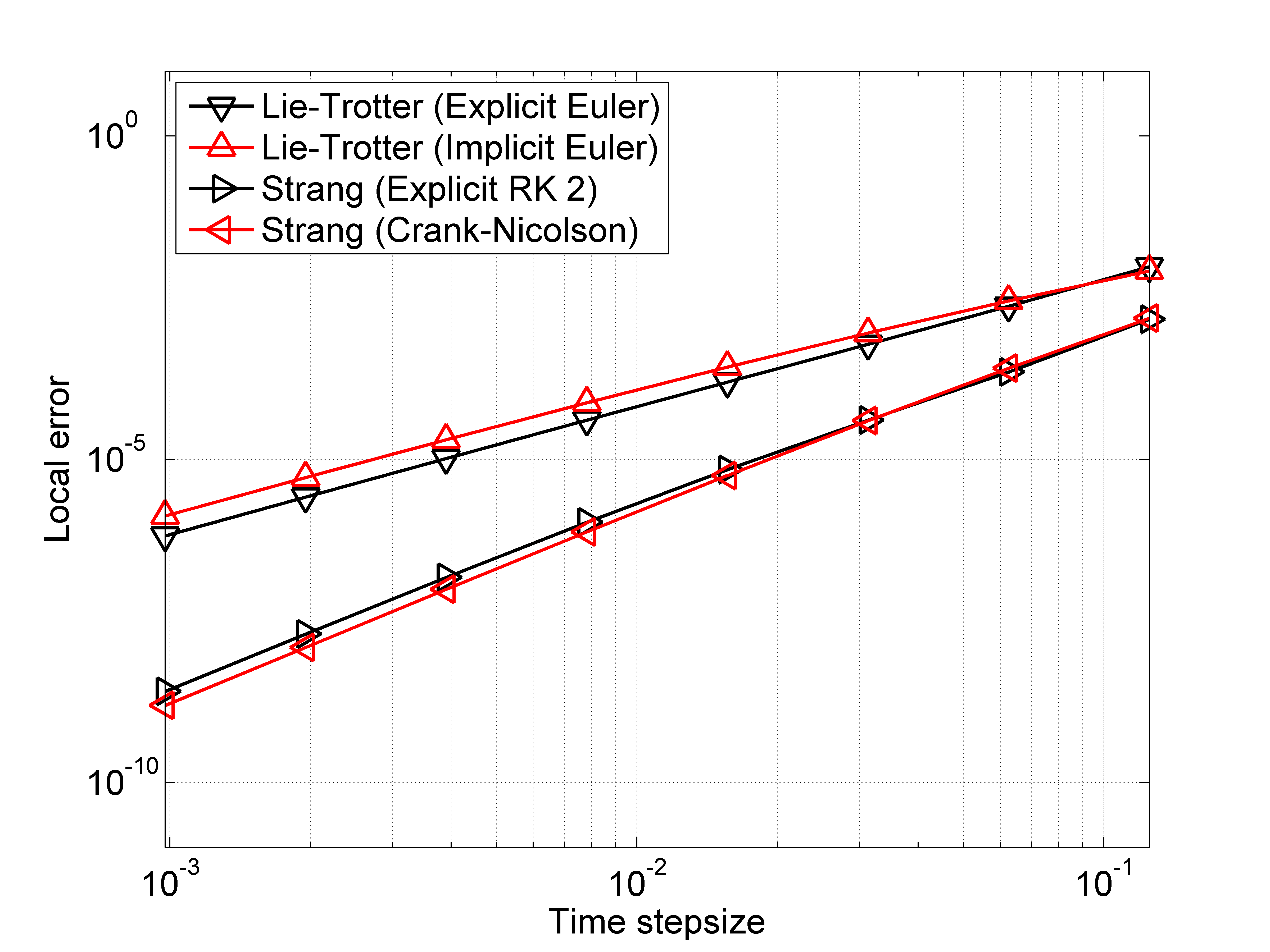
Figure 1: Local (left) and global (right) errors for the Lie–Trotter and Strang splitting methods with respect to the L2×L2L^{2}\times L^{2}-norm obtained for Decomposition I. Comparison of different time integration methods for the numerical solution of the subproblems.
Refer to caption
Refer to caption
Figure 2: Local (left) and global (right) errors for the Lie–Trotter and Strang splitting methods with respect to the H3×H1H^{3}\times H^{1}-norm obtained for Decomposition I. Comparison of different time integration methods for the numerical solution of the subproblems.
Refer to caption
Refer to caption
Refer to caption
Refer to caption
Refer to caption
Refer to caption
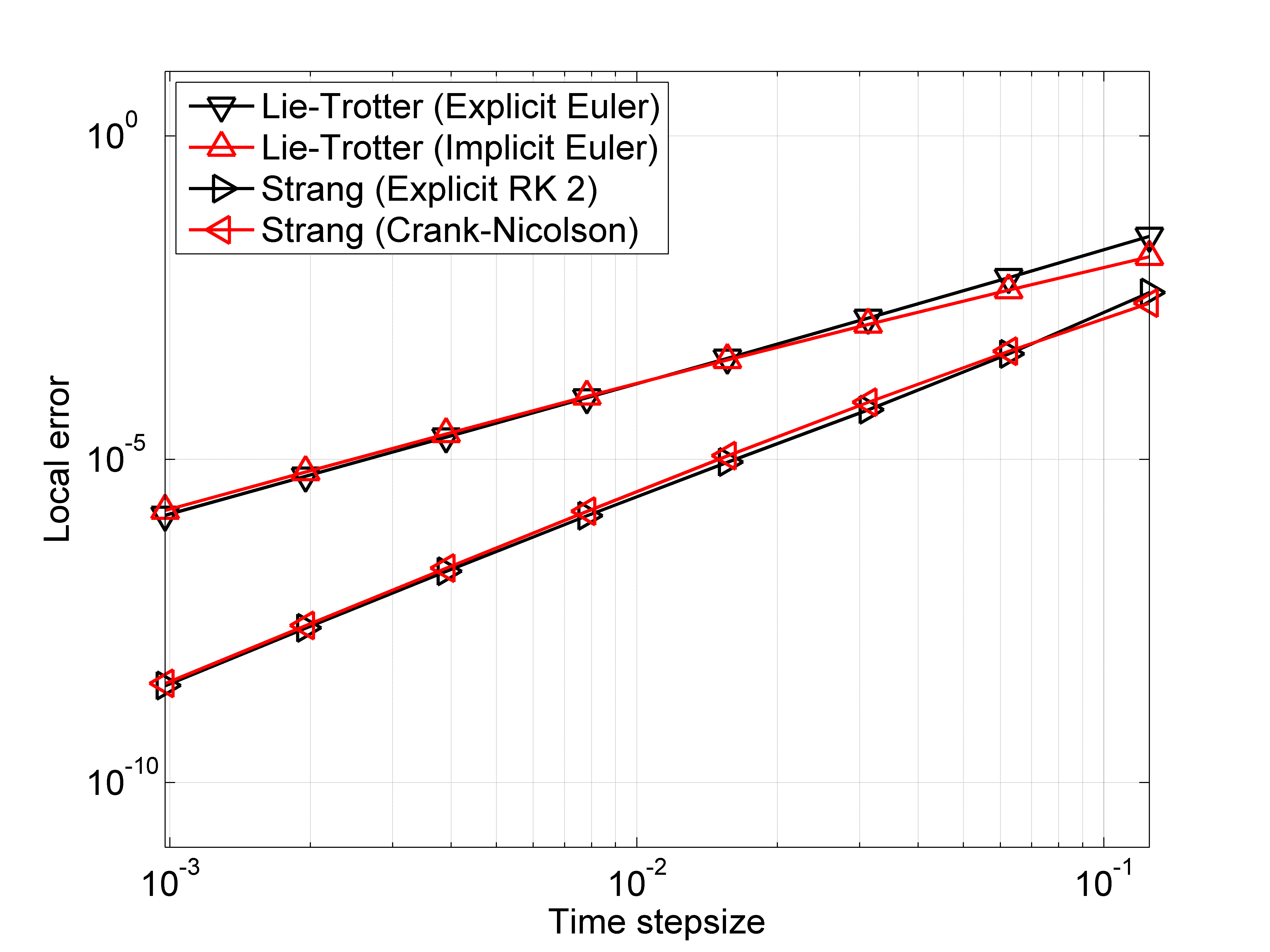
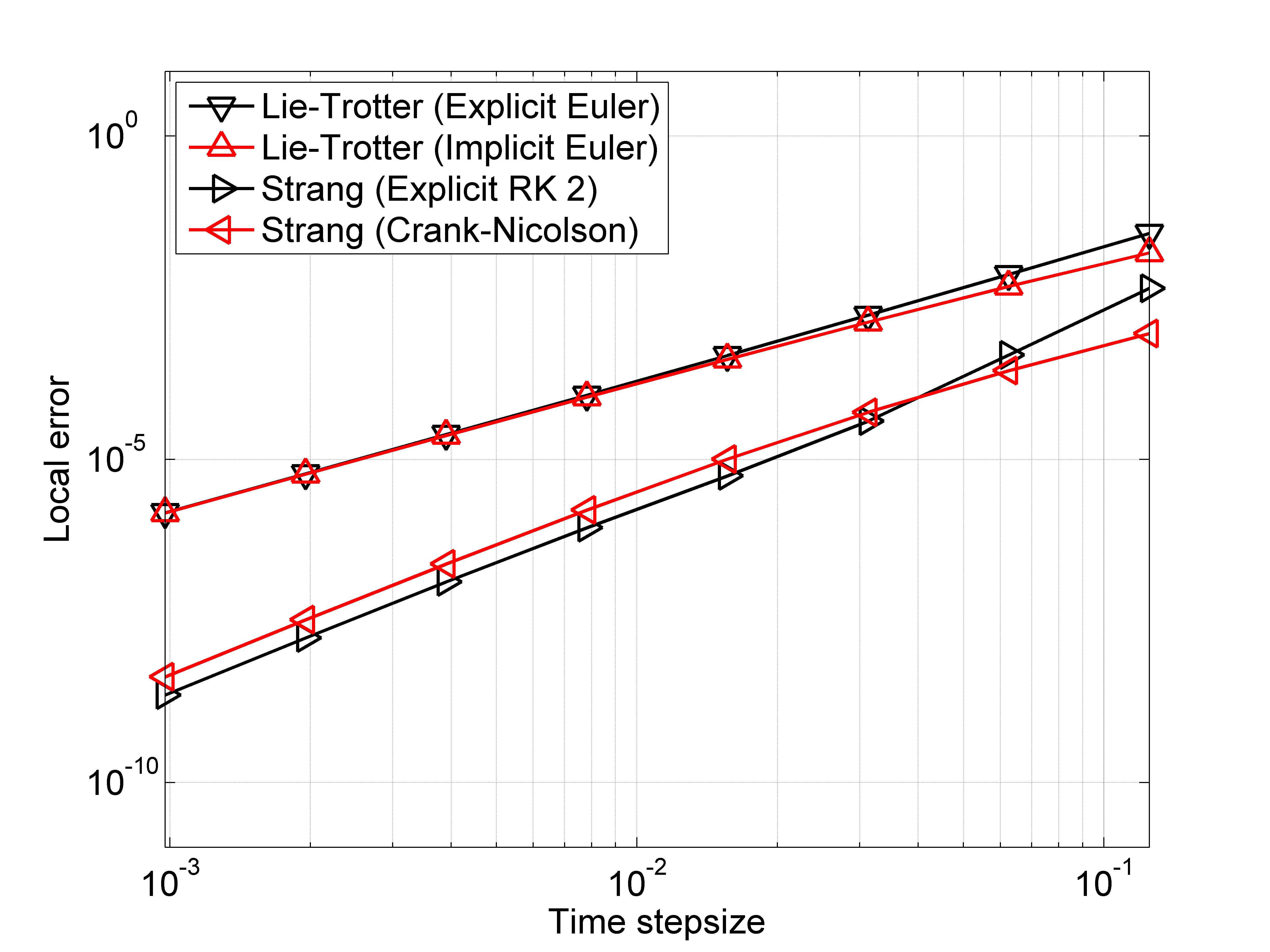
Figure 3: Local (left) and global (right) errors for the Lie–Trotter and Strang splitting methods with respect to the L2×L2L^{2}\times L^{2}-norm obtained for Decomposition II (first row), Decomposition III (second row) and Decomposition IV (third row). Comparison of different time integration methods for the numerical solution of the subproblems.
Refer to caption
Figure 4: Solution to the Westervelt equation with parameter values (6.2), computed by the Lie–Trotter splitting method based on Decomposition I. Comparison of the acoustic velocity potential with the solution to the linear wave equation at time 5⋅10−35\cdot 10^{-3}.
Model problem.

We consider the one-dimensional Westervelt equation

∂t​tψ⁡(x,t)−α​∂x​x​tψ⁡(x,t)−β​∂x​xψ⁡(x,t)=δ∂tψ(x,t)∂t​tψ(x,t),(x,t)∈(−a,a)×(0,T],\begin{split}&\partial_{tt}\psi(x,t)-\alpha\,\partial_{xxt}\psi(x,t)-\beta\,\partial_{xx}\psi(x,t)\\ &\quad=\delta\,\partial_{t}\psi(x,t)\,\partial_{tt}\psi(x,t)\,,\quad(x,t)\in(-a,a)\times(0,T]\,,\\ \end{split} (6.1a)
with parameter values
α=1,β=1,γ=12,δ=2​γ=1,\alpha=1\,,\qquad\beta=1\,,\qquad\gamma=\tfrac{1}{2}\,,\qquad\delta=2\gamma=1\,, (6.1b)
subject to homogeneous Dirichlet conditions
ψ⁡(−a,t)=0=ψ⁡(a,t),t∈[0,T],\psi(-a,t)=0=\psi(a,t)\,,\quad t\in[0,T]\,, (6.1c)
and regular initial conditions
ψ⁡(x,0)=e−x2,∂tψ⁡(x,0)=−x​e−x2,x∈[−a,a].\psi(x,0)={\rm e}^{-x^{2}}\,,\quad\partial_{t}\psi(x,0)=-\,x\,{\rm e}^{-x^{2}}\,,\qquad x\in[-a,a]\,. (6.1d)

For the numerical computations we set a=8a=8, T=1T=1, and choose M=100M=100 equidistant space grid points. In Figures 1 and 3 we display the local and global errors with respect to the L2×L2L^{2}\times L^{2}-norm, obtained for the Lie-Trotter and the Stang splitting methods based on Decompositions I-IV. Accordingly to Theorem 5.1, for Decomposition I we also include the errors with respect to a stronger norm, the H3×H1H^{3}\times H^{1}-norm, see Figure 2. In all cases, the slopes of the lines reflect the convergence orders p=1p=1 for the Lie–Trotter splitting method and p=2p=2 for the Strang splitting method, respectively. From the numerical results we conclude that the application of Decompositions II-IV does not improve the size of the errors; for this reason, we favour Decomposition I with the least computational effort.

Realistic parameter values.

As a further illustration, we consider the one-dimensional Westervelt equation with more realistic parameter, geometry, and excitation values

a=15,α=10−2,c=103,β=c2=106,δ=2⋅10−4,ψ(x,0)=0.5e−10​(x−1)2,x∈[−a,a],∂tψ(x,0)=c∂xψ(x,0)=−10c(x−1)e−10​(x−1)2,x∈[−a,a],\begin{gathered}a=15\,,\quad\alpha=10^{-2}\,,\quad c=10^{3}\,,\quad\beta=c^{2}=10^{6}\,,\,\quad\delta=2\cdot 10^{-4}\,,\\ \psi(x,0)=0.5\,{\rm e}^{-10(x-1)^{2}}\,,\quad x\in[-a,a]\,,\\ \partial_{t}\psi(x,0)=c\,\partial_{x}\psi(x,0)=-10\,c\,(x-1)\,{\rm e}^{-10(x-1)^{2}}\,,\quad x\in[-a,a]\,,\end{gathered} (6.2)

in the MKS system of units. For the time discretisation we apply the Lie–Trotter splitting method, based on Decomposition I and the explicit Euler method, and for the space discretisation we use Fast Fourier techniques. In Figure 4, we display the numerical result for the acoustic velocity potential ψ\psi at time t=5⋅10−3t=5\cdot 10^{-3}, obtained for M=6⋅103M=6\cdot 10^{3} space grid points and N=5⋅104N=5\cdot 10^{4} time steps. In order to reveal the effect of nonlinearity, we also display the profile of the solution to the linear wave equation ∂t​tψ−c2​Δ​ψ=0\partial_{tt}\psi-c^{2}\Delta\,\psi=0; as typical in the nonlinear case, a slight one-sided steepening of the pulse over time while the wave travels to the left is observed, see also [Kaltenbacher(2007), Section 5.6.4].

7 Regularity results

In this section, we deduce regularity results for the Westervelt equation and related evolution equations of hyperbolic and parabolic type. The stated results, ensuring that certain smoothness properties of the initial state are inherited by the solution to the original problem, the subproblems, and the associated variational equations, respectively, are essential ingredients in our convergence analysis of operator splitting methods for the time integration of the Westervelt equation. We study the Westervelt equation subject to homogeneous Dirichlet boundary conditions on a regular domain Ω⊂ℝ3\Omega\subset\mathbb{R}^{3}. The results can be extended to other boundary conditions, in the context of the Westervelt equation see for instance [Clason et al.(2009)]; they litterally carry over to the cases Ω⊂ℝd\Omega\subset\mathbb{R}^{d} with d=1,2d=1,2, where in a single space dimension the continuous embedding H1​(Ω)↪𝒞⁡(Ω)H^{1}(\Omega)\hookrightarrow\mathscr{C}(\Omega) is utilised to deal with nonlinearities. Our approach for the Westervelt equation utilises a regularity result proven in [Kaltenbacher and Lasiecka(2009)] for a reformulation in terms of the acoustic pressure. Although results on well posedness and regularity with respect to space and time can be found in the literature, see for instance [Evans(2010), Thm 6, p. 412] for the hyperbolic case and [Evans(2010), Thm 6, p. 386] for the parabolic case, we carry out the proofs of the stated results, since on one hand we only need local in time estimates as well as high spatial but low temporal regularity and on the other hand coefficients will depend on time in our setting. We note that estimates such as

‖(ψ,∂tψ)‖𝒞⁡([0,T],Hk+5×Hk+4)≤C,k∈ℕ≥0,\big\|\big(\psi,\partial_{t}\psi\big)\big\|_{\mathscr{C}([0,T],H^{k+5}\times H^{k+4})}\leq C\,,\qquad k\in\mathbb{N}_{\geq 0}\,,

are at first deduced for even exponents k+5=2​ℓk+5=2\ell with ℓ∈ℕ≥0\ell\in\mathbb{N}_{\geq 0}; the corresponding assertions for non-even and, more generally, for non-integer exponents then follow from the exact interpolation theorem, which states that boundedness of F:X→YF:X\to Y and F:X~→Y~F:\widetilde{X}\to\widetilde{Y} implies boundedness of F:(X,X~)ϑ,q→(Y,Y~)ϑ,qF:(X,\widetilde{X})_{\vartheta,q}\to(Y,\widetilde{Y})_{\vartheta,q} for 0<ϑ<10<\vartheta<1 and 1<q<∞1<q<\infty, see [Adams and Fournier(2003), Thm 7.23].

7.1 Westervelt equation

Initial-boundary value problem and reformulation.

We consider (2.1a) under homogeneous Dirichlet boundary conditions on a regular domain

{(1−δ​∂tψ⁡(x,t))​∂t​tψ⁡(x,t)−α​Δ​∂tψ⁡(x,t)−β​Δ​ψ​(x,t)=0,(x,t)∈Ω×(0,T],ψ(x,t)=0,(x,t)∈∂Ω×[0,T],ψ(x,0)=ψ0(x),∂tψ(x,0)=ψ1(x),x∈Ω.\begin{cases}&\big(1-\delta\,\partial_{t}\psi(x,t)\big)\,\partial_{tt}\psi(x,t)-\alpha\,\Delta\,\partial_{t}\psi(x,t)-\beta\,\Delta\,\psi(x,t)\\ &\quad=0\,,\quad(x,t)\in\Omega\times(0,T]\,,\\ &\psi(x,t)=0\,,\quad(x,t)\in\partial\Omega\times[0,T]\,,\\ &\psi(x,0)=\psi^{0}(x)\,,\quad\partial_{t}\psi(x,0)=\psi^{1}(x)\,,\quad x\in\Omega\,.\end{cases} (7.1)

As a first step, we formulate the Westervelt equation in terms of the acoustic pressure, related to the acoustic velocity potential via

p⁡(x,t)=ϱ​∂tψ⁡(x,t),∂tψ⁡(x,t)=1ϱ​p​(x,t),(x,t)∈Ω¯×[0,T],p(x,t)=\varrho\,\partial_{t}\psi(x,t)\,,\quad\partial_{t}\psi(x,t)=\tfrac{1}{\varrho}\,p(x,t)\,,\quad(x,t)\in\overline{\Omega}\times[0,T]\,, (7.2a)
for a positive constant ϱ>0\varrho>0. Differentation of the Westervelt equation yields
−δ​(∂t​tψ⁡(x,t))2+(1−δ​∂tψ⁡(x,t))​∂t​t​tψ⁡(x,t)−α​Δ​∂t​tψ⁡(x,t)−β​Δ​∂tψ⁡(x,t)=0;-\,\delta\,\big(\partial_{tt}\psi(x,t)\big)^{2}+\big(1-\delta\,\partial_{t}\psi(x,t)\big)\,\partial_{ttt}\psi(x,t)-\alpha\,\Delta\,\partial_{tt}\psi(x,t)-\beta\,\Delta\,\partial_{t}\psi(x,t)=0\,;
substituting ∂tψ=1ϱ​p\partial_{t}\psi=\tfrac{1}{\varrho}\,p as well as ∂t​tψ=1ϱ​∂tp\partial_{tt}\psi=\tfrac{1}{\varrho}\,\partial_{t}p and ∂t​t​tψ=1ϱ​∂t​tp\partial_{ttt}\psi=\tfrac{1}{\varrho}\,\partial_{tt}p implies
−δϱ2​(∂tp⁡(x,t))2+(1−δϱ​p​(x,t))​1ϱ​∂t​tp⁡(x,t)−αϱ​Δ​∂tp⁡(x,t)−βϱ​Δ​p​(x,t)=0.-\tfrac{\delta}{\varrho^{2}}\,\big(\partial_{t}p(x,t)\big)^{2}+\big(1-\tfrac{\delta}{\varrho}\,p(x,t)\big)\,\tfrac{1}{\varrho}\,\partial_{tt}p(x,t)-\tfrac{\alpha}{\varrho}\,\Delta\,\partial_{t}p(x,t)-\tfrac{\beta}{\varrho}\,\Delta p(x,t)=0\,.
Altogether, we obtain the reformulation
{(1−δϱ​p​(x,t))​∂t​tp⁡(x,t)−α​Δ​∂tp⁡(x,t)−β​Δ​p​(x,t)=δϱ(∂tp(x,t))2,(x,t)∈Ω×(0,T],p(x,t)=0,(x,t)∈∂Ω×[0,T],p(x,0)=ϱψ1(x),x∈Ω,∂tp(x,0)=ϱ(1−δψ1(x))−1(αΔψ1(x)+βΔψ0(x)),x∈Ω.\begin{cases}&\big(1-\tfrac{\delta}{\varrho}\,p(x,t)\big)\,\partial_{tt}p(x,t)-\alpha\,\Delta\,\partial_{t}p(x,t)-\beta\,\Delta p(x,t)\\ &\quad=\tfrac{\delta}{\varrho}\big(\partial_{t}p(x,t)\big)^{2}\,,\quad(x,t)\in\Omega\times(0,T]\,,\\ &p(x,t)=0\,,\quad(x,t)\in\partial\Omega\times[0,T]\,,\\ &p(x,0)=\varrho\,\psi^{1}(x)\,,\quad x\in\Omega\,,\\ &\partial_{t}p(x,0)=\varrho\,\big(1-\delta\psi^{1}(x)\big)^{-1}\,\big(\alpha\,\Delta\psi^{1}(x)+\beta\Delta\psi^{0}(x)\big)\,,\quad x\in\Omega\,.\end{cases} (7.2b)
Non-degeneracy and regularity result.

Provided that the prescribed initial state satisfies the regularity assumptions

p⁡(⋅,0)∈H2​(Ω),∂tp⁡(⋅,0)∈H1​(Ω),∂t​tp⁡(⋅,0)∈L2​(Ω),p(\cdot,0)\in H^{2}(\Omega)\,,\quad\partial_{t}p(\cdot,0)\in H^{1}(\Omega)\,,\quad\partial_{tt}p(\cdot,0)\in L^{2}(\Omega)\,, (7.3a)
with sufficiently small norms, the regularity result [Kaltenbacher and Lasiecka(2009), Thm 1.1] ensures non-degeneracy as well as local existence and uniqueness of a solution to a weak form of (7.2b), that is, there exist constants 0<ν¯<ν¯<∞0<\underline{\nu}<\overline{\nu}<\infty such that the relation
ν¯≤1−δϱ​p​(x,t)≤ν¯,(x,t)∈Ω¯×[0,T],\underline{\nu}\leq 1-\tfrac{\delta}{\varrho}\,p(x,t)\leq\overline{\nu}\,,\qquad(x,t)\in\overline{\Omega}\times[0,T]\,, (7.3b)
holds and furthermore
p∈𝒞⁡([0,T],H2​(Ω))∩𝒞1​([0,T],H1​(Ω))∩𝒞2​([0,T],L2​(Ω))∩H2​((0,T),H1​(Ω)).\begin{split}&p\in\mathscr{C}\big([0,T],H^{2}(\Omega)\big)\cap\mathscr{C}^{1}\big([0,T],H^{1}(\Omega)\big)\cap\mathscr{C}^{2}\big([0,T],L^{2}(\Omega)\big)\\ &\qquad\qquad\cap H^{2}\big((0,T),H^{1}(\Omega)\big)\,.\end{split} (7.3c)
Regularity result.

The above statement permits to deduce the following regularity result for the Westervelt equation. We note that the proof of Theorem 7.1 via  [Kaltenbacher and Lasiecka(2009), Thms 1.2, 1.3] ensures well-posedness, globally in time, that is, there exist positive constants ρ>0\rho>0 and M>0M>0 such that the energy norm remains bounded

Eψ,1(t)=12(∥∂t​t​tψ(⋅,t)∥L22+∥∇∂t​tψ(⋅,t)∥L22+∥Δ∂tψ(⋅,t)∥L22)≤M,t≥0,E_{\psi,1}(t)=\tfrac{1}{2}\Big(\big\|\partial_{ttt}\psi(\cdot,t)\big\|_{L^{2}}^{2}+\big\|\nabla\partial_{tt}\psi(\cdot,t)\big\|_{L^{2}}^{2}+\big\|\Delta\,\partial_{t}\psi(\cdot,t)\big\|_{L^{2}}^{2}\Big)\leq M\,,\qquad t\geq 0\,,

provided that Eψ,1​(0)≤ρE_{\psi,1}(0)\leq\rho; moreover, due to the strong damping present in the equation, the energy decays exponentially. However, for our purposes it suffices to prove local well-posedness and regularity results.

Theorem 7.1.

Let T>0T>0 and M>0M>0 be arbitrary.

  1. (i)

    There exists a constant ρ>0\rho>0 such that if the initial data fulfill the regularity and compatibility assumptions

    ψ0,ψ1∈H01​(Ω)∩H4​(Ω),‖(ψ0,ψ1)‖H4×H4=‖ψ0‖H4+‖ψ1‖H4≤ρ,∂t​tψ⁡(⋅,0)=(1−δ​ψ1)−1​(α​Δ​ψ1+β​Δ​ψ0)∈H01​(Ω)∩H2​(Ω),\begin{gathered}\psi^{0},\psi^{1}\in H_{0}^{1}(\Omega)\cap H^{4}(\Omega)\,,\qquad\big\|\big(\psi^{0},\psi^{1}\big)\big\|_{H^{4}\times H^{4}}=\big\|\psi^{0}\big\|_{H^{4}}+\big\|\psi^{1}\big\|_{H^{4}}\leq\rho\,,\\ \partial_{tt}\psi(\cdot,0)=\big(1-\delta\psi^{1}\big)^{-1}\big(\alpha\,\Delta\psi^{1}+\beta\,\Delta\psi^{0}\big)\in H_{0}^{1}(\Omega)\cap H^{2}(\Omega)\,,\end{gathered}

    then the solution to the Westervelt equation (7.1) exists and satisfies the non-degeneracy condition

    ν¯≤1−δ​∂tψ⁡(x,t)≤ν¯,(x,t)∈Ω¯×[0,T],\underline{\nu}\leq 1-\delta\,\partial_{t}\psi(x,t)\leq\overline{\nu}\,,\qquad(x,t)\in\overline{\Omega}\times[0,T]\,,

    with some constants 0<ν¯<ν¯<∞0<\underline{\nu}<\overline{\nu}<\infty; moreover, the relation

    ψ∈𝒞1​([0,T],H4​(Ω))∩𝒞2​([0,T],H2​(Ω))∩𝒞3​([0,T],L2​(Ω))∩H3​((0,T),H1​(Ω))\begin{split}&\psi\in\mathscr{C}^{1}\big([0,T],H^{4}(\Omega)\big)\cap\mathscr{C}^{2}\big([0,T],H^{2}(\Omega)\big)\cap\mathscr{C}^{3}\big([0,T],L^{2}(\Omega)\big)\\ &\qquad\qquad\cap H^{3}\big((0,T),H^{1}(\Omega)\big)\end{split}

    and the bound

    ‖(ψ⁡(⋅,t),∂tψ⁡(⋅,t),∂t​tψ⁡(⋅,t))‖H4×H4×H2≤eC​t​‖(ψ0,ψ1)‖H4×H4,t∈[0,T],\begin{split}&\big\|\big(\psi(\cdot,t),\partial_{t}\psi(\cdot,t),\partial_{tt}\psi(\cdot,t)\big)\big\|_{H^{4}\times H^{4}\times H^{2}}\leq{\rm e}^{Ct}\,\big\|\big(\psi^{0},\psi^{1}\big)\big\|_{H^{4}\times H^{4}}\,,\\ &\qquad t\in[0,T]\,,\end{split}

    are valid.

  2. (ii)

    For every m∈ℕ≥2m\in\mathbb{N}_{\geq 2} there exists a constant ρ>0\rho>0 such that if the initial data fulfull the regularity and compatibility assumptions

    (ψ0,ψ1)∈H2​(m+1)(Ω)×H2​m+1(Ω),∥(ψ0,ψ1)∥H2​(m+1)×H2​m+1≤ρ,∂t​tΔk​ψ​(⋅,0)=(1−δ​ψ1)−1​(α​Δk+1​ψ1+β​Δk+1​ψ0)+fk​(⋅,0)∈H01​(Ω),\begin{gathered}\big(\psi^{0},\psi^{1}\big)\in H^{2(m+1)}(\Omega)\times H^{2m+1}(\Omega)\,,\qquad\big\|\big(\psi^{0},\psi^{1}\big)\big\|_{H^{2(m+1)}\times H^{2m+1}}\leq\rho\,,\\ \partial_{tt}\Delta^{k}\psi(\cdot,0)=\big(1-\delta\psi^{1}\big)^{-1}\big(\alpha\Delta^{k+1}\psi^{1}+\beta\Delta^{k+1}\psi^{0}\big)+f_{k}(\cdot,0)\in H_{0}^{1}(\Omega)\,,\end{gathered}

    for any integer 1≤k≤m1\leq k\leq m, where

    fk=Δk​((1−δ​∂tψ)−1​Δ​(α​∂tψ+β​ψ))−(1−δ​∂tψ)−1​Δk+1​(α​∂tψ+β​ψ),f_{k}=\Delta^{k}\Big(\big(1-\delta\partial_{t}\psi\big)^{-1}\Delta(\alpha\,\partial_{t}\psi+\beta\,\psi)\Big)-\big(1-\delta\partial_{t}\psi\big)^{-1}\Delta^{k+1}(\alpha\,\partial_{t}\psi+\beta\,\psi)\,,

    then the solution to (7.1) satisfies the relation

    (ψ,∂tψ)∈𝒞⁡([0,T],H2​(m+1)​(Ω)×H2​m+1​(Ω))\big(\psi,\partial_{t}\psi\big)\in\mathscr{C}\big([0,T],H^{2(m+1)}(\Omega)\times H^{2m+1}(\Omega)\big)

    and the bound

    ‖(ψ⁡(⋅,t),∂tψ⁡(⋅,t))‖H2​(m+1)×H2​m+1≤eC​t​‖(ψ0,ψ1)‖H2​(m+1)×H2​m+1.\big\|\big(\psi(\cdot,t),\partial_{t}\psi(\cdot,t)\big)\big\|_{H^{2(m+1)}\times H^{2m+1}}\leq{\rm e}^{Ct}\,\big\|\big(\psi^{0},\psi^{1}\big)\big\|_{H^{2(m+1)}\times H^{2m+1}}\,.

Proof. For notational simplicity, for a function f:Ω¯×[0,T]→ℝf:\overline{\Omega}\times[0,T]\to\mathbb{R} we henceforth write f⁡(t)=f⁡(⋅,t)f(t)=f(\cdot,t) for short.

  1. (i)

    (a) Non-degeneracy. Inserting p=ϱ​∂tψp=\varrho\,\partial_{t}\psi into (7.3b) immediately implies

    0<ν¯≤(1−δ​∂tψ⁡(t))≤ν¯<∞,t∈[0,T].0<\underline{\nu}\leq\big(1-\delta\,\partial_{t}\psi(t)\big)\leq\overline{\nu}<\infty\,,\qquad t\in[0,T]\,.

    (b) Basic regularity. For convenience, we recall the relations

    ∂tp=ϱ​∂t​tψ=ϱ​(1−δ​∂tψ)−1​(α​Δ​∂tψ+β​Δ​ψ),∂t​tp=(1−δϱ​p)−1​(α​Δ​∂tp+β​Δ​p+δϱ​(∂tp)2),\begin{split}\partial_{t}p&=\varrho\,\partial_{tt}\psi=\varrho\,\big(1-\delta\,\partial_{t}\psi\big)^{-1}\,\big(\alpha\,\Delta\,\partial_{t}\psi+\beta\,\Delta\,\psi\big)\,,\\ \partial_{tt}p&=\big(1-\tfrac{\delta}{\varrho}\,p\big)^{-1}\,\big(\alpha\,\Delta\,\partial_{t}p+\beta\,\Delta p+\tfrac{\delta}{\varrho}\big(\partial_{t}p\big)^{2}\big)\,,\end{split}

    see also (7.1)–(7.2). The assumption ψ0,ψ1∈H4​(Ω)\psi^{0},\psi^{1}\in H^{4}(\Omega) ensures that the initial data

    p⁡(0)=ϱ​ψ1,∂tp⁡(0)=ϱ​(1−δ​ψ1)−1​(α​Δ​ψ1+β​Δ​ψ0),∂t​tp⁡(0)=(1−δϱ​p​(0))−1​(α​Δ​∂tp⁡(0)+β​Δ​p​(0)+δϱ​(∂tp⁡(0))2)=ϱ​(1−δ​ψ1)−1​(α​Δ​((1−δ​ψ1)−1​(α​Δ​ψ1+β​Δ​ψ0))+β​Δ​ψ1CLOSEOPEN+δ​(1−δ​ψ1)−2​(α​Δ​ψ1+β​Δ​ψ0)2),\begin{split}p(0)&=\varrho\,\psi^{1}\,,\\ \partial_{t}p(0)&=\varrho\,\big(1-\delta\,\psi^{1}\big)^{-1}\,\big(\alpha\,\Delta\psi^{1}+\beta\,\Delta\psi^{0}\big)\,,\\ \partial_{tt}p(0)&=\big(1-\tfrac{\delta}{\varrho}\,p(0)\big)^{-1}\,\big(\alpha\,\Delta\,\partial_{t}p(0)+\beta\,\Delta p(0)+\tfrac{\delta}{\varrho}\,\big(\partial_{t}p(0)\big)^{2}\big)\\ &=\varrho\,\big(1-\delta\,\psi^{1}\big)^{-1}\,\Big(\alpha\,\Delta\,\big(\big(1-\delta\,\psi^{1}\big)^{-1}\,\big(\alpha\,\Delta\psi^{1}+\beta\,\Delta\psi^{0}\big)\big)+\beta\,\Delta\,\psi^{1}\\ &\qquad+\delta\,\big(1-\delta\,\psi^{1}\big)^{-2}\,\big(\alpha\,\Delta\psi^{1}+\beta\,\Delta\psi^{0}\big)^{2}\Big)\,,\end{split}

    chosen accordingly, fulfill the requirements

    p⁡(0)∈H2​(Ω),∂tp⁡(0)∈H1​(Ω),∂t​tp⁡(0)∈L2​(Ω);p(0)\in H^{2}(\Omega)\,,\qquad\partial_{t}p(0)\in H^{1}(\Omega)\,,\qquad\partial_{tt}p(0)\in L^{2}(\Omega)\,;

    an application of the regularity result (7.3) thus implies

    p∈𝒞⁡([0,T],H2​(Ω))∩𝒞1​([0,T],H1​(Ω))∩𝒞2​([0,T],L2​(Ω))∩H2​((0,T),H1​(Ω)).\begin{split}&p\in\mathscr{C}\big([0,T],H^{2}(\Omega)\big)\cap\mathscr{C}^{1}\big([0,T],H^{1}(\Omega)\big)\cap\mathscr{C}^{2}\big([0,T],L^{2}(\Omega)\big)\\ &\qquad\qquad\cap H^{2}\big((0,T),H^{1}(\Omega)\big)\,.\end{split}

    Together with the relation

    ψ⁡(t)=ψ0+1ρ​∫0tp⁡(τ)​𝑑τ,\psi(t)=\psi^{0}+\tfrac{1}{\rho}\int_{0}^{t}p(\tau)\;{\rm d}\tau\,,

    obtained by integrating ∂tψ=1ϱ​p\partial_{t}\psi=\tfrac{1}{\varrho}\,p in time, this proves

    ψ∈𝒞1​([0,T],H2​(Ω))∩𝒞2​([0,T],H1​(Ω))∩𝒞3​([0,T],L2​(Ω))∩H3​((0,T),H1​(Ω)).\begin{split}&\psi\in\mathscr{C}^{1}\big([0,T],H^{2}(\Omega)\big)\cap\mathscr{C}^{2}\big([0,T],H^{1}(\Omega)\big)\cap\mathscr{C}^{3}\big([0,T],L^{2}(\Omega)\big)\\ &\qquad\qquad\cap H^{3}\big((0,T),H^{1}(\Omega)\big)\,.\end{split} (7.4)

    (c) Additional regularity. Continuous Sobolev embeddings (5.1) imply

    ‖(1−δ​∂tψ⁡(t))​∂t​tψ⁡(t)‖H1≤C⁡(1+‖ψ‖𝒞1​([0,T],H2))​‖ψ‖𝒞2​([0,T],H1),\big\|\big(1-\delta\,\partial_{t}\psi(t)\big)\,\partial_{tt}\psi(t)\big\|_{H^{1}}\leq C\,\big(1+\|\psi\|_{\mathscr{C}^{1}([0,T],H^{2})}\big)\,\|\psi\|_{\mathscr{C}^{2}([0,T],H^{1})}\,,

    and thus by (7.1) we get

    f=α​Δ​∂tψ+β​Δ​ψ=(1−δ​∂tψ)​∂t​tψ∈𝒞⁡([0,T],H1​(Ω)).f=\alpha\,\Delta\,\partial_{t}\psi+\beta\,\Delta\,\psi=\big(1-\delta\,\partial_{t}\psi\big)\,\partial_{tt}\psi\in\mathscr{C}\big([0,T],H^{1}(\Omega)\big)\,.

    Making use of the fact that Δ​ψ\Delta\,\psi fulfills the differential equation

    ∂tΔ​ψ​(t)=−βα​Δ​ψ​(t)+1α​f​(t),\partial_{t}\Delta\,\psi(t)=-\tfrac{\beta}{\alpha}\,\Delta\,\psi(t)+\tfrac{1}{\alpha}\,f(t)\,, (7.5a)
    employing the linear variation-of-constants formula
    Δ​ψ​(t)=e−βα​t​Δ​ψ0+1α​∫0te−βα​(t−s)​f​(s)​𝑑s,\Delta\,\psi(t)={\rm e}^{-\frac{\beta}{\alpha}t}\Delta\psi^{0}+\tfrac{1}{\alpha}\int_{0}^{t}{\rm e}^{-\frac{\beta}{\alpha}(t-s)}f(s)\;{\rm d}s\,, (7.5b)

    and recalling that the initial state satisfies ψ0∈H4​(Ω)\psi^{0}\in H^{4}(\Omega), we conclude that the relations Δ​ψ​(t)∈H1​(Ω)\Delta\,\psi(t)\in H^{1}(\Omega) and by (7.5) OPENΔ​∂tψ⁡(t)∈H1​(Ω))\Delta\,\partial_{t}\psi(t)\in H^{1}(\Omega)) are valid, that is, we obtain

    (ψ,∂tψ)∈𝒞⁡([0,T],H3​(Ω)×H3​(Ω)).\big(\psi,\partial_{t}\psi\big)\in\mathscr{C}\big([0,T],H^{3}(\Omega)\times H^{3}(\Omega)\big)\,.

    A reformulation of the Westervelt equation and differentiation in time leads to

    −αΔ∂tψ=β​Δ​ψ−(1−δ​∂tψ)​∂t​tψ,−αΔ∂t​tψ=β​Δ​∂tψ+δ​(∂t​tψ)2−(1−δ​∂tψ)​∂t​t​tψ,α​∂t​tψ=(−Δ)−1(−αΔ∂t​tψ)=−β∂tψ+(−Δ)−1(δ(∂t​tψ)2−(1−δ∂tψ)∂t​t​tψ);\begin{split}-\,\alpha\,\Delta\,\partial_{t}\psi&=\beta\,\Delta\,\psi-\big(1-\delta\,\partial_{t}\psi\big)\,\partial_{tt}\psi\,,\\ -\,\alpha\,\Delta\,\partial_{tt}\psi&=\beta\,\Delta\,\partial_{t}\psi+\delta\,\big(\partial_{tt}\psi\big)^{2}-\big(1-\delta\,\partial_{t}\psi\big)\,\partial_{ttt}\psi\,,\\ \alpha\,\partial_{tt}\psi&=(-\Delta)^{-1}\,\big(-\alpha\,\Delta\,\partial_{tt}\psi\big)\\ &=-\beta\,\partial_{t}\psi+(-\Delta)^{-1}\Big(\delta\,\big(\partial_{tt}\psi\big)^{2}-\big(1-\delta\,\partial_{t}\psi\big)\,\partial_{ttt}\psi\Big)\,;\end{split}

    due to the the compatibility condition ∂t​tψ⁡(0)∈H01​(Ω)∩H2​(Ω)\partial_{tt}\psi(0)\in H^{1}_{0}(\Omega)\cap H^{2}(\Omega) an application of the Laplace operator under homogeneous Dirichlet boundary conditions to ∂t​tψ\partial_{tt}\psi is justified. Consequently, the relation

    f=(1−δ​∂tψ)​∂t​tψ=1α(1−δ∂tψ)(−β∂tψOPEN+(−Δ)−1​(δ​(∂t​tψ)2−(1−δ​∂tψ)​∂t​t​tψ))\begin{split}f&=\big(1-\delta\,\partial_{t}\psi\big)\,\partial_{tt}\psi\\ &=\tfrac{1}{\alpha}\,\big(1-\delta\,\partial_{t}\psi\big)\,\Big(-\beta\,\partial_{t}\psi\\ &\qquad+(-\Delta)^{-1}\Big(\delta\,\big(\partial_{tt}\psi\big)^{2}-\big(1-\delta\,\partial_{t}\psi\big)\,\partial_{ttt}\psi\Big)\Big)\end{split}

    follows. By the above considerations ∂tψ∈𝒞⁡([0,T],H3​(Ω))\partial_{t}\psi\in\mathscr{C}\big([0,T],H^{3}(\Omega)\big) and by (7.4) the relations ∂t​tψ∈𝒞⁡([0,T],H1​(Ω))\partial_{tt}\psi\in\mathscr{C}([0,T],H^{1}(\Omega)) and ∂t​t​tψ∈𝒞⁡([0,T],L2​(Ω))\partial_{ttt}\psi\in\mathscr{C}\big([0,T],L^{2}(\Omega)\big) hold; together with the regularisation (−Δ)−1:L2​(Ω)→H2​(Ω)(-\Delta)^{-1}:L^{2}(\Omega)\to H^{2}(\Omega) and continuous Sobolev embeddings (5.1) we obtain

    ‖f⁡(t)‖H2≤C​‖1−δ​∂tψ⁡(t)‖H2​(‖∂tψ⁡(t)‖H2+‖∂t​tψ⁡(t)‖H12CLOSEOPEN+‖1−δ​∂tψ⁡(t)‖H2​‖∂t​t​tψ⁡(t)‖L2),\begin{split}\|f(t)\|_{H^{2}}&\leq C\,\big\|1-\delta\,\partial_{t}\psi(t)\big\|_{H^{2}}\Big(\big\|\partial_{t}\psi(t)\big\|_{H^{2}}+\big\|\partial_{tt}\psi(t)\big\|_{H^{1}}^{2}\\ &\qquad+\big\|1-\delta\,\partial_{t}\psi(t)\big\|_{H^{2}}\,\|\partial_{ttt}\psi(t)\|_{L^{2}}\Big)\,,\end{split}

    which implies

    f∈𝒞⁡([0,T],H2​(Ω)).f\in\mathscr{C}\big([0,T],H^{2}(\Omega)\big)\,.

    Proceeding as above, via (7.5) we conclude that Δ​ψ,Δ​∂tψ∈𝒞⁡([0,T],H2​(Ω))\Delta\,\psi\,,\Delta\,\partial_{t}\psi\in\mathscr{C}([0,T],H^{2}(\Omega)) holds and finally obtain

    (ψ,∂tψ)∈𝒞⁡([0,T],H4​(Ω)×H4​(Ω)).\big(\psi,\partial_{t}\psi\big)\in\mathscr{C}\big([0,T],H^{4}(\Omega)\times H^{4}(\Omega)\big)\,.

    (d) Additional regularity. We utilise the relation

    Δ​∂t​tψ=Δ⁡((1−δ​∂tψ)−1)​(α​Δ​∂tψ+β​Δ​ψ)+2∇((1−δ∂tψ)−1)⋅(α∇Δ∂tψ+β∇Δψ)+(1−δ​∂tψ)−1​(α​Δ2​∂tψ+β​Δ2​ψ),\begin{split}\Delta\,\partial_{tt}\psi&=\Delta\big(\big(1-\delta\,\partial_{t}\psi\big)^{-1}\big)\,\big(\alpha\,\Delta\,\partial_{t}\psi+\beta\,\Delta\,\psi\big)\\ &\qquad+2\,\nabla\big(\big(1-\delta\,\partial_{t}\psi\big)^{-1}\big)\cdot\big(\alpha\,\nabla\Delta\,\partial_{t}\psi+\beta\,\nabla\Delta\,\psi\big)\\ &\qquad+\big(1-\delta\,\partial_{t}\psi\big)^{-1}\,\big(\alpha\,\Delta^{2}\,\partial_{t}\psi+\beta\,\Delta^{2}\psi\big)\,,\end{split}

    which results from an application of the Laplace operator to the Westervelt equation and the identity Δ(fg)=Δfg+2∇f⋅∇g+fΔg\Delta(fg)=\Delta f\,g+2\,\nabla f\cdot\nabla g+f\,\Delta g. Estimation by continuous Sobolev embeddings (5.1) implies

    ‖Δ​∂t​tψ⁡(t)‖L2≤C​‖Δ⁡((1−δ​∂tψ⁡(t))−1)‖L2​(‖Δ​∂tψ⁡(t)‖L∞+‖Δ​ψ​(t)‖L∞)+C​‖∇((1−δ​∂tψ⁡(t))−1)‖L4×(∥∇Δ∂tψ(t)∥L4+∥∇Δψ(t)∥L4)+C​‖(1−δ​∂tψ⁡(t))−1‖L∞×(‖Δ2​∂tψ⁡(t)‖L2+‖Δ2​ψ​(t)‖L2)≤C​‖(1−δ​∂tψ⁡(t))−1‖H2​(‖ψ⁡(t)‖H4+‖∂tψ⁡(t)‖H4)\begin{split}\big\|\Delta\,\partial_{tt}\psi(t)\big\|_{L^{2}}&\leq C\,\big\|\Delta\big(\big(1-\delta\,\partial_{t}\psi(t)\big)^{-1}\big)\big\|_{L^{2}}\,\Big(\big\|\Delta\,\partial_{t}\psi(t)\big\|_{L^{\infty}}+\big\|\Delta\,\psi(t)\big\|_{L^{\infty}}\Big)\\ &\qquad+C\,\big\|\nabla\big(\big(1-\delta\,\partial_{t}\psi(t)\big)^{-1}\big)\big\|_{L^{4}}\\ &\qquad\qquad\times\Big(\big\|\nabla\Delta\,\partial_{t}\psi(t)\big\|_{L^{4}}+\big\|\nabla\Delta\,\psi(t)\big\|_{L^{4}}\Big)\\ &\qquad+C\,\big\|\big(1-\delta\,\partial_{t}\psi(t)\big)^{-1}\big\|_{L^{\infty}}\\ &\qquad\qquad\times\Big(\big\|\Delta^{2}\,\partial_{t}\psi(t)\big\|_{L^{2}}+\big\|\Delta^{2}\psi(t)\big\|_{L^{2}}\Big)\\ &\leq C\,\big\|\big(1-\delta\,\partial_{t}\psi(t)\big)^{-1}\big\|_{H^{2}}\,\Big(\big\|\psi(t)\big\|_{H^{4}}+\big\|\partial_{t}\psi(t)\big\|_{H^{4}}\Big)\end{split}

    and due to (ψ,∂tψ)∈𝒞⁡([0,T],H4​(Ω)×H4​(Ω))\big(\psi,\partial_{t}\psi\big)\in\mathscr{C}\big([0,T],H^{4}(\Omega)\times H^{4}(\Omega)\big) proves

    ∂t​tψ∈𝒞⁡([0,T],H2​(Ω)).\partial_{tt}\psi\in\mathscr{C}\big([0,T];H^{2}(\Omega)\big)\,.
  2. (ii)

    Higher regularity. In order to prove the stated higher regularity of the solution to the Westervelt equation, we proceed by induction, employing the regularity result deduced in the previous step. That is, we consider the partial differential equation for χ=Δm​ψ\chi=\Delta^{m}\psi obtained from an m−m-fold application of the Laplace operator to the Westervelt equation under homogeneous Dirichlet boundary conditions

    {∂t​tχ(t)=α^(t)Δ∂tχ(t)+β^(t)Δχ(t)+fm(t),t∈(0,T],χ(t)|∂Ω=0,t∈[0,T],χ(0)=Δmψ0,∂tχ(0)=Δmψ1,\begin{cases}&\partial_{tt}\chi(t)=\widehat{\alpha}(t)\,\Delta\,\partial_{t}\,\chi(t)+\widehat{\beta}(t)\,\Delta\chi(t)+f_{m}(t)\,,\quad t\in(0,T]\,,\\ &\chi(t)\big|_{\partial\Omega}=0\,,\quad t\in[0,T]\,,\qquad\chi(0)=\Delta^{m}\psi^{0}\,,\quad\partial_{t}\chi(0)=\Delta^{m}\psi^{1}\,,\end{cases} (7.6)

    which is justified by the required compatibility conditions; here, we write

    α^=α​δ^,β^=β​δ^,δ^=(1−δ​∂tψ)−1,\widehat{\alpha}=\alpha\,\widehat{\delta}\,,\qquad\widehat{\beta}=\beta\,\widehat{\delta}\,,\qquad\widehat{\delta}=(1-\delta\partial_{t}\psi)^{-1}\,,

    for short and use the following reformulation of the right-hand side

    Δm​(α^​Δ​∂tψ+β^​Δ​ψ)=Δm​(δ^​Δ​(α​∂tψ+β​ψ))=δ^​Δm+1​(α​∂tψ+β​ψ)+fm=α^​Δ​∂tχ+β^​Δ​χ+fm\begin{split}\Delta^{m}\big(\widehat{\alpha}\,\Delta\,\partial_{t}\psi+\widehat{\beta}\,\Delta\,\psi\big)&=\Delta^{m}\big(\widehat{\delta}\,\Delta(\alpha\,\partial_{t}\psi+\beta\,\psi)\big)=\widehat{\delta}\,\Delta^{m+1}(\alpha\,\partial_{t}\psi+\beta\,\psi)+f_{m}\\ &=\widehat{\alpha}\,\Delta\,\partial_{t}\chi+\widehat{\beta}\,\Delta\chi+f_{m}\end{split}

    involving

    fm=Δm(δ^g)−δ^Δmg=∑j=12​m(2​mj)∇jδ^⋅∇2​m−jg,g=Δ(α∂tψ+βψ)).f_{m}=\Delta^{m}(\widehat{\delta}\,g)-\widehat{\delta}\,\Delta^{m}g=\sum_{j=1}^{2m}\,\tbinom{2m}{j}\nabla^{j}\widehat{\delta}\,\cdot\nabla^{2m-j}g\,,\qquad g=\Delta(\alpha\,\partial_{t}\psi+\beta\,\psi)\big)\,.

    In order to show that

    (χ,∂tχ)=(Δm​ψ,Δm​∂tψ)∈𝒞⁡([0,T],H2​(Ω)×H1​(Ω)),m∈ℕ≥2,\big(\chi,\partial_{t}\chi)=\big(\Delta^{m}\psi,\Delta^{m}\partial_{t}\psi\big)\in\mathscr{C}\big([0,T],H^{2}(\Omega)\times H^{1}(\Omega)\big)\,,\qquad m\in\mathbb{N}_{\geq 2}\,,

    or, equivalently,

    (ψ,∂tψ)∈𝒞⁡([0,T],H2​(m+1)​(Ω)×H2​m+1​(Ω)),m∈ℕ≥2,\big(\psi,\partial_{t}\psi\big)\in\mathscr{C}\big([0,T],H^{2(m+1)}(\Omega)\times H^{2m+1}(\Omega)\big)\,,\qquad m\in\mathbb{N}_{\geq 2}\,,

    holds, we carry out an induction proof with respect to integer 2≤k≤m2\leq k\leq m for the assertion

    (ψ,∂tψ)∈𝒞⁡([0,T],H2​(k+1)​(Ω)×H2​k+1​(Ω)),‖(ψ,∂tψ)‖𝒞⁡(H2​(k+1)×H2​k+1)≤C​‖(ψ0,ψ1)‖H2​(k+1)×H2​k+1,\begin{gathered}\big(\psi,\partial_{t}\psi\big)\in\mathscr{C}\big([0,T],H^{2(k+1)}(\Omega)\times H^{2k+1}(\Omega)\big)\,,\\ \big\|\big(\psi,\partial_{t}\psi\big)\big\|_{\mathscr{C}(H^{2(k+1)}\times H^{2k+1})}\leq C\,\big\|\big(\psi^{0},\psi^{1}\big)\big\|_{H^{2(k+1)}\times H^{2k+1}}\,,\end{gathered} (7.7a)
    based on the induction hypothesis
    (ψ,∂tψ)∈𝒞⁡(H2​k​(Ω)×H2​k−1​(Ω)),‖(ψ,∂tψ)‖𝒞⁡(H2​k×H2​k−1)≤C​‖(ψ0,ψ1)‖H2​k×H2​k−1;\begin{gathered}\big(\psi,\partial_{t}\psi\big)\in\mathscr{C}\big(H^{2k}(\Omega)\times H^{2k-1}(\Omega)\big)\,,\\ \big\|\big(\psi,\partial_{t}\psi\big)\big\|_{\mathscr{C}(H^{2k}\times H^{2k-1})}\leq C\,\big\|\big(\psi^{0},\psi^{1}\big)\big\|_{H^{2k}\times H^{2k-1}}\,;\end{gathered} (7.7b)
    our previous considerations ensure that the induction beginning
    (ψ,∂tψ)∈𝒞⁡(H4​(Ω)×H4​(Ω)),‖(ψ,∂tψ)‖𝒞⁡(H4×H4)≤C​‖(ψ0,ψ1)‖H4×H4,\begin{gathered}\big(\psi,\partial_{t}\psi\big)\in\mathscr{C}\big(H^{4}(\Omega)\times H^{4}(\Omega)\big)\,,\\ \big\|\big(\psi,\partial_{t}\psi\big)\big\|_{\mathscr{C}(H^{4}\times H^{4})}\leq C\,\big\|\big(\psi^{0},\psi^{1}\big)\big\|_{H^{4}\times H^{4}}\,,\end{gathered} (7.7c)

    is valid. A fundamental regularity result for linear evolution equations of hyperbolic type is given below in Proposition 7.2; applying the first statement of Proposition 7.2 to (7.6) with mm replaced by kk, noting that by (7.7b)–(7.7c) and the required smallness of the initial data the conditions

    a=α^,c=β^≥ν>0,b=0,c=β^∈H1((0,T),L∞(Ω)),f=fk∈L2((0,T),L2(Ω)),\begin{gathered}a=\widehat{\alpha}\,,\qquad c=\widehat{\beta}\geq\nu>0\,,\\ b=0\,,\qquad c=\widehat{\beta}\in H^{1}\big((0,T),L^{\infty}(\Omega)\big)\,,\qquad f=f_{k}\in L^{2}\big((0,T),L^{2}(\Omega)\big)\,,\end{gathered}

    are fulfilled, we obtain

    ‖(Δk​ψ,Δk​∂tψ)‖𝒞⁡([0,T],H2×H1)≤C⁡((1+‖∂tβ^‖L2​((0,T),L∞))​‖(Δk​ψ0,Δk​ψ1)‖H2×H1CLOSEOPEN+‖fk‖L2​((0,T),L2))≤C⁡((1+‖(ψ0,ψ1)‖H4×H4)​‖(Δk​ψ0,Δk​ψ1)‖H2×H1CLOSEOPEN+‖fk‖L2​((0,T),L2)),\begin{split}&\big\|\big(\Delta^{k}\psi,\Delta^{k}\partial_{t}\psi\big)\big\|_{\mathscr{C}([0,T],H^{2}\times H^{1})}\\ &\qquad\leq C\,\Big(\big(1+\big\|\partial_{t}\widehat{\beta}\big\|_{L^{2}((0,T),L^{\infty})}\big)\,\big\|\big(\Delta^{k}\psi^{0},\Delta^{k}\psi^{1}\big)\big\|_{H^{2}\times H^{1}}\\ &\qquad\qquad\quad+\big\|f_{k}\big\|_{L^{2}((0,T),L^{2})}\Big)\\ &\qquad\leq C\,\Big(\big(1+\big\|\big(\psi^{0},\psi^{1}\big)\big\|_{H^{4}\times H^{4}}\big)\,\big\|\big(\Delta^{k}\psi^{0},\Delta^{k}\psi^{1}\big)\big\|_{H^{2}\times H^{1}}\\ &\qquad\qquad\quad+\big\|f_{k}\big\|_{L^{2}((0,T),L^{2})}\Big)\,,\end{split} (7.8)

    since the following bound holds

    ‖∂tβ^‖L2​((0,T),L∞)≤β​δν¯2​‖∂t​tψ‖L2​((0,T),L∞)≤C​‖(ψ0,ψ1)‖H4×H4.\big\|\partial_{t}\widehat{\beta}\big\|_{L^{2}((0,T),L^{\infty})}\leq\tfrac{\beta\delta}{\underline{\nu}^{2}}\,\big\|\partial_{tt}\psi\big\|_{L^{2}((0,T),L^{\infty})}\leq C\,\big\|\big(\psi^{0},\psi^{1}\big)\big\|_{H^{4}\times H^{4}}\,.

    It remains to estimate

    ‖fk‖L2​((0,T),L2)≤∑j=12​k‖∇jδ^⋅∇2​k−jΔ​(α​∂tψ+β​ψ)‖L2​((0,T),L2).\big\|f_{k}\big\|_{L^{2}((0,T),L^{2})}\leq\sum_{j=1}^{2k}\big\|\nabla^{j}\widehat{\delta}\cdot\nabla^{2k-j}\Delta(\alpha\partial_{t}\psi+\beta\,\psi)\big\|_{L^{2}((0,T),L^{2})}\,.

    For this purpose, we first consider the contribution δ^=δ~​(∂tψ)\widehat{\delta}=\widetilde{\delta}(\partial_{t}\psi) involving the scalar function

    δ~:ℝ∖{δ−1}⟶ℝ:ζ⟼11−δ​ζ;\widetilde{\delta}:\mathbb{R}\setminus\{\delta^{-1}\}\longrightarrow\mathbb{R}:\zeta\longmapsto\frac{1}{1-\delta\zeta}\,;

    we note that non-degeneracy is essential for the regularity of δ~\widetilde{\delta}. By (7.7b)–(7.7c) we have ∂tψ∈𝒞⁡([0,T],𝒞j​(Ω¯))\partial_{t}\psi\in\mathscr{C}([0,T],\mathscr{C}^{j}(\overline{\Omega})) for any j≤max⁡{2,2​k−3}j\leq\max\{2,2k-3\} and thus

    ‖δ^‖𝒞⁡([0,T],Wj,∞)≤supt∈[0,T]supκ∈ℕ≥03|n|≤j​supx∈Ω¯|∂xκ(1−δ​∂tψ⁡(x,t))−1|≤C​‖δ~‖𝒞j​([ν¯−1,ν¯−1])​supt∈[0,T]‖∂tψ⁡(t)‖𝒞j​(Ω¯)≤C​‖δ~‖𝒞j​([ν¯−1,ν¯−1])​‖∂tψ‖𝒞⁡([0,T],Hj+2);\begin{split}\big\|\widehat{\delta}\big\|_{\mathscr{C}([0,T],W^{j,\infty})}&\leq\sup_{t\in[0,T]}\underset{|n|\leq j}{\sup_{\kappa\in\mathbb{N}_{\geq 0}^{3}}}\sup_{x\in\overline{\Omega}}\big|\partial_{x}^{\kappa}\big(1-\delta\,\partial_{t}\psi(x,t)\big)^{-1}\big|\\ &\leq C\,\big\|\widetilde{\delta}\big\|_{\mathscr{C}^{j}([\overline{\nu}^{-1},\underline{\nu}^{-1}])}\,\sup_{t\in[0,T]}\big\|\partial_{t}\psi(t)\big\|_{\mathscr{C}^{j}(\overline{\Omega})}\\ &\leq C\,\big\|\widetilde{\delta}\big\|_{\mathscr{C}^{j}([\overline{\nu}^{-1},\underline{\nu}^{-1}])}\,\big\|\partial_{t}\psi\big\|_{\mathscr{C}([0,T],H^{j+2})}\,;\end{split}

    the highest derivatives of δ^\widehat{\delta} can be estimated utilising ∇δ^=δδ^ 2∇∂tψ\nabla\widehat{\delta}=\delta\,\widehat{\delta}^{\,2}\nabla\partial_{t}\psi and

    ∇jδ^=δ∇j−1(δ^ 2∇∂tψ)=δ∑i=0j−1(j−1i)∇iδ^ 2∇j−i∂tψ=δ​∑i=0j−1(j−1i)​∑ℓ=0i(iℓ)​∇ℓδ^​∇i−ℓδ^​∇j−i​∂tψ.\begin{split}\nabla^{j}\widehat{\delta}&=\delta\,\nabla^{j-1}\big(\widehat{\delta}^{\,2}\nabla\partial_{t}\psi\big)=\delta\sum_{i=0}^{j-1}\tbinom{j-1}{i}\,\nabla^{i}\widehat{\delta}^{\,2}\,\nabla^{j-i}\,\partial_{t}\psi\\ &=\delta\sum_{i=0}^{j-1}\tbinom{j-1}{i}\sum_{\ell=0}^{i}\tbinom{i}{\ell}\nabla^{\ell}\widehat{\delta}\,\nabla^{i-\ell}\widehat{\delta}\,\nabla^{j-i}\partial_{t}\psi\,.\end{split}

    For j=2​k−2j=2k-2, j=2​k−1j=2k-1, and j=2​kj=2k we get

    ∇2​k−2δ^=δ​∑i=12​k−3(2​k−3i)​∇iδ^ 2​∇2​k−2−i​∂tψ⏟G1+δ​δ^ 2⏟G1​∇2​k−2∂tψ⏟G2,∇2​k−1δ^=δ​∑i=22​k−3(2​k−2i)​∇iδ^ 2​∇2​k−1−i​∂tψ⏟G1+δ​δ^ 2⏟G1​∇2​k−1∂tψ⏟G3+δ(2k−2)∇δ^ 2⏟G1​∇2​k−2∂tψ⏟G2+δ​∇2​k−2​δ^ 2⏟G2​∇∂tψ⏟G1,∇2​kδ^=δ​∑i=32​k−3(2​k−1i)​∇iδ^ 2​∇2​k−i​∂tψ⏟G1+δ​δ^ 2⏟G1​∇2​k∂tψ⏟G4+δ(2k−1)∇δ^ 2⏟G1​∇2​k−1∂tψ⏟G3+δ​(2​k−12)​∇2δ^ 2⏟G1​∇2​k−2∂tψ⏟G2+δ⁡(2​k−1)​∇2​k−2δ^ 2⏟G2​∇2∂tψ⏟G1+δ​∇2​k−1​δ^ 2⏟G3​∇∂tψ⏟G1,\begin{split}\nabla^{2k-2}\widehat{\delta}&=\underbrace{\delta\sum_{i=1}^{2k-3}\tbinom{2k-3}{i}\,\nabla^{i}\widehat{\delta}^{\,2}\,\nabla^{2k-2-i}\,\partial_{t}\psi}_{G_{1}}+\underbrace{\delta\,\widehat{\delta}^{\,2}}_{G_{1}}\underbrace{\nabla^{2k-2}\,\partial_{t}\psi}_{G_{2}}\,,\\ \nabla^{2k-1}\widehat{\delta}&=\underbrace{\delta\sum_{i=2}^{2k-3}\tbinom{2k-2}{i}\,\nabla^{i}\widehat{\delta}^{\,2}\,\nabla^{2k-1-i}\,\partial_{t}\psi}_{G_{1}}+\underbrace{\delta\,\widehat{\delta}^{\,2}}_{G_{1}}\underbrace{\nabla^{2k-1}\,\partial_{t}\psi}_{G_{3}}\\ &\qquad+\underbrace{\delta\,(2k-2)\nabla\,\widehat{\delta}^{\,2}}_{G_{1}}\underbrace{\nabla^{2k-2}\,\partial_{t}\psi}_{G_{2}}+\underbrace{\delta\,\nabla^{2k-2}\,\widehat{\delta}^{\,2}}_{G_{2}}\underbrace{\nabla\partial_{t}\psi}_{G_{1}}\,,\\ \nabla^{2k}\widehat{\delta}&=\underbrace{\delta\sum_{i=3}^{2k-3}\tbinom{2k-1}{i}\nabla^{i}\,\widehat{\delta}^{\,2}\,\nabla^{2k-i}\,\partial_{t}\psi}_{G_{1}}+\underbrace{\delta\,\widehat{\delta}^{\,2}}_{G_{1}}\underbrace{\nabla^{2k}\,\partial_{t}\psi}_{G_{4}}\\ &\qquad+\underbrace{\delta\,(2k-1)\,\nabla\widehat{\delta}^{\,2}}_{G_{1}}\underbrace{\nabla^{2k-1}\,\partial_{t}\psi}_{G_{3}}\,+\underbrace{\delta\,\tbinom{2k-1}{2}\nabla^{2}\,\widehat{\delta}^{\,2}}_{G_{1}}\underbrace{\nabla^{2k-2}\,\partial_{t}\psi}_{G_{2}}\\ &\qquad+\underbrace{\delta\,(2k-1)\nabla^{2k-2}\,\widehat{\delta}^{\,2}}_{G_{2}}\underbrace{\nabla^{2}\,\partial_{t}\psi}_{G_{1}}\,+\underbrace{\delta\,\nabla^{2k-1}\,\widehat{\delta}^{\,2}}_{G_{3}}\underbrace{\nabla\partial_{t}\psi}_{G_{1}}\,,\end{split}

    involving quantities that have in common that they satisfy

    G1∈𝒞([0,T],L∞(Ω)),G2∈𝒞([0,T],L6(Ω)),G3∈𝒞([0,T],L2(Ω)),G4∈L2((0,T),L2(Ω)),\begin{gathered}G_{1}\in\mathscr{C}\big([0,T],L^{\infty}(\Omega)\big)\,,\qquad G_{2}\in\mathscr{C}\big([0,T],L^{6}(\Omega)\big)\,,\\ G_{3}\in\mathscr{C}\big([0,T],L^{2}(\Omega)\big)\,,\qquad G_{4}\in L^{2}\big((0,T),L^{2}(\Omega)\big)\,,\end{gathered}

    with G1,G2,G3G_{1},G_{2},G_{3} bounded provided that ∂tψ\partial_{t}\psi is bounded in 𝒞⁡([0,T],Hmax⁡{4,2​k−1}​(Ω))\mathscr{C}([0,T],H^{\max\{4,2k-1\}}(\Omega)) and G4G_{4} bounded whenever Δk​∂tψ\Delta^{k}\partial_{t}\psi is bounded in L2​((0,T),L2​(Ω))L^{2}((0,T),L^{2}(\Omega)). Using once more (7.7b)–(7.7c) implies

    ‖∂tψ‖𝒞⁡([0,T],Hmax⁡{4,2​k−1})≤C​‖(ψ0,ψ1)‖H2​k×Hmax⁡{4,2​k−1},\big\|\partial_{t}\psi\big\|_{\mathscr{C}([0,T],H^{\max\{4,2k-1\}})}\leq C\,\|\big(\psi^{0},\psi^{1}\big)\|_{H^{2k}\times H^{\max\{4,2k-1\}}}\,,

    and thus we obtain the estimate

    ‖fk‖L2​((0,T),L2)≤C​‖(ψ0,ψ1)‖H2​k×Hmax⁡{4,2​k−1}​(1+‖Δk​∂tψ‖L2​((0,T),L2CLOSE)≤C​‖(ψ0,ψ1)‖H2​k×Hmax⁡{4,2​k−1}​(1+‖Δk​∂tψ‖𝒞⁡([0,T],H1CLOSE).\begin{split}\|f_{k}\|_{L^{2}((0,T),L^{2})}&\leq C\,\big\|\big(\psi^{0},\psi^{1}\big)\big\|_{H^{2k}\times H^{\max\{4,2k-1\}}}\,\big(1+\big\|\Delta^{k}\partial_{t}\psi\big\|_{L^{2}((0,T),L^{2}}\big)\\ &\leq C\,\big\|\big(\psi^{0},\psi^{1}\big)\big\|_{H^{2k}\times H^{\max\{4,2k-1\}}}\,\big(1+\big\|\Delta^{k}\partial_{t}\psi\big\|_{\mathscr{C}([0,T],H^{1}}\big)\,.\end{split}

    Inserting into (7.8), this finally implies the relation

    ‖(Δk​ψ,Δk​∂tψ)‖𝒞⁡([0,T],H2×H1)≤C⁡((1+‖(ψ0,ψ1)‖H4×H4)​‖(Δk​ψ0,Δk​ψ1)‖H2×H1CLOSEOPEN+‖(ψ0,ψ1)‖H2​k×Hmax⁡{4,2​k−1}​(1+‖Δk​∂tψ‖𝒞⁡([0,T],H1CLOSE));\begin{split}&\big\|\big(\Delta^{k}\psi,\Delta^{k}\partial_{t}\psi\big)\big\|_{\mathscr{C}([0,T],H^{2}\times H^{1})}\\ &\qquad\leq C\,\Big(\big(1+\big\|\big(\psi^{0},\psi^{1}\big)\big\|_{H^{4}\times H^{4}}\big)\,\big\|\big(\Delta^{k}\psi^{0},\Delta^{k}\psi^{1}\big)\big\|_{H^{2}\times H^{1}}\\ &\qquad\qquad+\big\|\big(\psi^{0},\psi^{1}\big)\big\|_{H^{2k}\times H^{\max\{4,2k-1\}}}\,\big(1+\big\|\Delta^{k}\partial_{t}\psi\big\|_{\mathscr{C}([0,T],H^{1}}\big)\Big)\,;\end{split}

    by restricting the size of the inital data the condition

    ‖(ψ0,ψ1)‖OPENH2​k×Hmax⁡{4,2​k−1})<12​C\begin{split}\big\|\big(\psi^{0},\psi^{1}\big)\big\|_{H^{2k}\times H^{\max\{4,2k-1\}})}<\tfrac{1}{2C}\end{split}

    can be fulfilled. Altogether, this implies (7.7a) and concludes the proof. ♢\hfill\diamondsuit

7.2 Linear evolution equations of hyperbolic type

Regularity result.

In the following, we state a regularity result for a linear wave equation subject to homogeneous Dirichlet boundary conditions on a regular domain

{∂t​tψ⁡(x,t)=a⁡(x,t)​Δ​∂tψ⁡(x,t)+b⁡(x,t)​∂tψ⁡(x,t)+c⁡(x,t)​Δ​ψ​(x,t)+f⁡(x,t),(x,t)∈Ω×(0,T],ψ(x,t)=0,(x,t)∈∂Ω×[0,T],ψ(x,0)=ψ0(x),∂tψ(x,0)=ψ1(x),x∈Ω.\begin{cases}&\partial_{tt}\psi(x,t)=a(x,t)\,\Delta\,\partial_{t}\psi(x,t)+b(x,t)\,\partial_{t}\psi(x,t)\\ &\qquad\qquad\qquad+\;c(x,t)\,\Delta\,\psi(x,t)+f(x,t)\,,\quad(x,t)\in\Omega\times(0,T]\,,\\ &\psi(x,t)=0\,,\quad(x,t)\in\partial\Omega\times[0,T]\,,\\ &\psi(x,0)=\psi^{0}(x)\,,\quad\partial_{t}\psi(x,0)=\psi^{1}(x)\,,\quad x\in\Omega\,.\end{cases} (7.9)

We note that in the present context the coefficient bb may have arbitrary sign and thus the term b​∂tψb\,\partial_{t}\psi cannot be regarded as a damping term.

Proposition 7.2.

Assume that the coefficient functions satisfy the positivity and regularity conditions

a⁡(x,t),c⁡(x,t)≥ν>0,(x,t)∈Ω×[0,T],b∈L2((0,T),L3(Ω)),c∈W1,1((0,T),L∞(Ω)),f∈L2((0,T),L2(Ω)),\begin{gathered}a(x,t)\,,\,c(x,t)\geq\nu>0\,,\qquad(x,t)\in\Omega\times[0,T]\,,\\ b\in L^{2}\big((0,T),L^{3}(\Omega)\big)\,,\quad c\in W^{1,1}\big((0,T),L^{\infty}(\Omega)\big)\,,\quad f\in L^{2}\big((0,T),L^{2}(\Omega)\big)\,,\end{gathered}

with ‖b‖L2​((0,T),L3)\|b\|_{L^{2}((0,T),L^{3})} and ‖∂tc‖L2​((0,T),L∞)\|\partial_{t}c\|_{L^{2}((0,T),L^{\infty})} sufficiently small.

  1. (i)

    Then the solution to (7.9) satisfies the relation

    (ψ,∂tψ)∈𝒞⁡([0,T],H2​(Ω)×H1​(Ω))\big(\psi,\partial_{t}\psi\big)\in\mathscr{C}\big([0,T],H^{2}(\Omega)\times H^{1}(\Omega)\big)

    and the bound

    ‖(ψ,∂tψ)‖𝒞⁡([0,T],H2×H1)≤C⁡(‖(ψ0,ψ1)‖H2×H1+‖f‖L2​((0,T),L2))\big\|\big(\psi,\partial_{t}\psi\big)\big\|_{\mathscr{C}([0,T],H^{2}\times H^{1})}\leq C\,\big(\big\|\big(\psi^{0},\psi^{1}\big)\big\|_{H^{2}\times H^{1}}+\big\|f\big\|_{L^{2}((0,T),L^{2})}\big)

    with constant depending on the respective norms of bb and cc, but not on aa.

  2. (ii)

    If in addition the relations

    a∈L2((0,T),W1,∞(Ω)∩W2,3(Ω)),b∈L2((0,T),H2(Ω)),c∈L2​((0,T),H2​(Ω))∩H1​((0,T),L∞​(Ω)),f∈𝒞([0,T],H01(Ω))∩L2((0,T),H2(Ω)),ψ1∈H01(Ω),∂t​tψ⁡(⋅,0)=a⁡(⋅,0)​Δ​ψ1+b⁡(⋅,0)​ψ1+c⁡(⋅,0)​Δ​ψ0+f⁡(⋅,0)∈H01​(Ω),\begin{gathered}a\in L^{2}\big((0,T),W^{1,\infty}(\Omega)\cap W^{2,3}(\Omega)\big)\,,\quad b\in L^{2}\big((0,T),H^{2}(\Omega)\big)\,,\\ c\in L^{2}\big((0,T),H^{2}(\Omega)\big)\cap H^{1}\big((0,T),L^{\infty}(\Omega)\big)\,,\\ f\in\mathscr{C}\big([0,T],H_{0}^{1}(\Omega)\big)\cap L^{2}\big((0,T),H^{2}(\Omega)\big)\,,\qquad\psi^{1}\in H_{0}^{1}(\Omega)\,,\\ \partial_{tt}\psi(\cdot,0)=a(\cdot,0)\,\Delta\psi^{1}+b(\cdot,0)\,\psi^{1}+c(\cdot,0)\,\Delta\psi^{0}+f(\cdot,0)\in H_{0}^{1}(\Omega)\,,\end{gathered}

    are satisfied and the norms

    ‖a‖L2​((0,T),W1,∞),‖b‖L2​((0,T),H1),‖c‖L2​((0,T),H2),\big\|a\big\|_{L^{2}((0,T),W^{1,\infty})}\,,\qquad\big\|b\big\|_{L^{2}((0,T),H^{1})}\,,\qquad\big\|c\big\|_{L^{2}((0,T),H^{2})}\,,

    are sufficiently small, then the solution to (7.9) satisfies the relation

    (ψ,∂tψ)∈𝒞⁡([0,T],H4​(Ω)×H3​(Ω))\big(\psi,\partial_{t}\psi\big)\in\mathscr{C}\big([0,T],H^{4}(\Omega)\times H^{3}(\Omega)\big)

    and the bound

    ‖(ψ,∂tψ)‖𝒞⁡([0,T],H4×H3)≤C⁡(‖(ψ0,ψ1)‖H4×H3+‖f‖L2​((0,T),H2))\big\|\big(\psi,\partial_{t}\psi\big)\big\|_{\mathscr{C}([0,T],H^{4}\times H^{3})}\leq C\,\big(\big\|\big(\psi^{0},\psi^{1}\big)\big\|_{H^{4}\times H^{3}}+\big\|f\big\|_{L^{2}((0,T),H^{2})}\big)

    with constant depending on the respective norms of a,b,ca,b,c. If additionally

    b∈L2​((0,T),W1,∞​(Ω)∩W2,3​(Ω)),b\in L^{2}\big((0,T),W^{1,\infty}(\Omega)\cap W^{2,3}(\Omega)\big)\,,

    then smallness of ‖b‖L2​((0,T),H1)\|b\|_{L^{2}((0,T),H^{1})} is not required.

Proof.

As before, for a function f:Ω¯×[0,T]→ℝf:\overline{\Omega}\times[0,T]\to\mathbb{R} we write f⁡(t)=f⁡(⋅,t)f(t)=f(\cdot,t) for short.

  1. (i)

    Multiplication of the partial differential equation by Δ​∂tψ\Delta\,\partial_{t}\psi, integration with respect to space and time, and application of integration-by-parts yields

    12∥∇∂tψ(t)∥L22+∫0t∥a⁡(τ)Δ∂tψ(τ)∥L22dτ+12∥cΔψ(t)∥L22=12​‖∇ψ1‖L22+12​‖c​Δ​ψ0‖L22+∫0t∫Ω(12∂tc(τ)(Δψ(τ))2−(f(τ)+b(τ)∂tψ(τ))Δ∂tψ(τ))dτ.\begin{split}&\tfrac{1}{2}\,\big\|\nabla\partial_{t}\psi(t)\big\|_{L^{2}}^{2}+\int_{0}^{t}\big\|\sqrt{a(\tau)}\,\Delta\,\partial_{t}\psi(\tau)\big\|_{L^{2}}^{2}\;{\rm d}\tau+\tfrac{1}{2}\,\big\|\sqrt{c}\,\Delta\,\psi(t)\big\|_{L^{2}}^{2}\\ &\qquad=\tfrac{1}{2}\,\big\|\nabla\psi^{1}\big\|_{L^{2}}^{2}+\tfrac{1}{2}\,\big\|\sqrt{c}\,\Delta\psi^{0}\big\|_{L^{2}}^{2}\\ &\qquad\qquad+\int_{0}^{t}\int_{\Omega}\Big(\tfrac{1}{2}\,\partial_{t}c(\tau)\,\big(\Delta\,\psi(\tau)\big)^{2}-\big(f(\tau)+b(\tau)\,\partial_{t}\psi(\tau)\big)\,\Delta\,\partial_{t}\psi(\tau)\Big)\;{\rm d}\tau\,.\end{split}

    Estimation by Hölder’s and Young’s inequality implies on the one hand

    ∫0t∫Ω12​∂tc⁡(τ)​(Δ​ψ​(τ))2​𝑑τ=∫0t∫Ω12​∂tc⁡(τ)c⁡(τ)​(c⁡(τ)​Δ​ψ​(τ))2​𝑑τ≤ν−1​‖∂tc‖L1​((0,T),L∞)​supτ∈[0,t]‖c​Δ​ψ​(τ)‖L22\begin{split}&\int_{0}^{t}\int_{\Omega}\tfrac{1}{2}\,\partial_{t}c(\tau)\,\big(\Delta\,\psi(\tau)\big)^{2}\;{\rm d}\tau=\int_{0}^{t}\int_{\Omega}\tfrac{1}{2}\,\frac{\partial_{t}c(\tau)}{c(\tau)}\,\big(\sqrt{c(\tau)}\,\Delta\,\psi(\tau)\big)^{2}\;{\rm d}\tau\\ &\qquad\leq\nu^{-1}\,\big\|\partial_{t}c\big\|_{L^{1}((0,T),L^{\infty})}\,\sup_{\tau\in[0,t]}\big\|\sqrt{c}\,\Delta\,\psi(\tau)\big\|_{L^{2}}^{2}\end{split}

    and on the other hand

    −∫0t∫Ω(f(τ)+b(τ)∂tψ(τ))Δ∂tψ(τ)dτ≤‖f+b​∂tψa‖L2​((0,t),L2)​‖a​Δ​∂tψ‖L2​((0,t),L2)≤(2​ν)−1​‖f‖L2​((0,T),L2)2+(2​ν)−1​‖b‖L2​((0,T),L3)2​supτ∈[0,t]‖∂tψ⁡(τ)‖L62+‖a​Δ​∂tψ‖L2​((0,t),L2)2,\begin{split}&-\int_{0}^{t}\int_{\Omega}\big(f(\tau)+b(\tau)\,\partial_{t}\psi(\tau)\big)\,\Delta\,\partial_{t}\psi(\tau)\;{\rm d}\tau\\ &\qquad\leq\Big\|\frac{f+b\,\partial_{t}\psi}{\sqrt{a}}\Big\|_{L^{2}((0,t),L^{2})}\,\big\|\sqrt{a}\,\Delta\,\partial_{t}\psi\big\|_{L^{2}((0,t),L^{2})}\\ &\qquad\leq(2\nu)^{-1}\,\big\|f\big\|_{L^{2}((0,T),L^{2})}^{2}+(2\nu)^{-1}\,\big\|b\big\|_{L^{2}((0,T),L^{3})}^{2}\,\sup_{\tau\in[0,t]}\big\|\partial_{t}\psi(\tau)\big\|_{L^{6}}^{2}\\ &\qquad\qquad+\big\|\sqrt{a}\,\Delta\,\partial_{t}\psi\big\|_{L^{2}((0,t),L^{2})}^{2}\,,\end{split}

    since (x1+x2)​x3=x1​x3+x2​x3≤12​x12+12​x22+x32(x_{1}+x_{2})\,x_{3}=x_{1}x_{3}+x_{2}x_{3}\leq\frac{1}{2}x_{1}^{2}+\frac{1}{2}x_{2}^{2}+x_{3}^{2} for x1,x2,x3∈ℝx_{1},x_{2},x_{3}\in\mathbb{R}, involving a constant that depends on ν−1\nu^{-1}; hence, using that the term involving a​Δ​∂tψ\sqrt{a}\,\Delta\,\partial_{t}\psi cancels out, we obtain

    12∥∇∂tψ(t)∥L22+12∥cΔψ(t)∥L22≤12​‖∇ψ1‖L22+12​‖c​Δ​ψ0‖L22+ν−1|∂tc|supτ∈[0,t]L1​((0,T),L∞)⁡‖c​Δ​ψ​(τ)‖L22+(2ν)−1∥f∥L2​((0,T),L2)2+(2ν)−1∥b∥L2​((0,T),L3)2supτ∈[0,t]∥∇∂tψ(τ)∥L22,\begin{split}&\tfrac{1}{2}\,\big\|\nabla\partial_{t}\psi(t)\big\|_{L^{2}}^{2}+\tfrac{1}{2}\,\big\|\sqrt{c}\,\Delta\,\psi(t)\big\|_{L^{2}}^{2}\\ &\quad\leq\tfrac{1}{2}\,\big\|\nabla\psi^{1}\big\|_{L^{2}}^{2}+\tfrac{1}{2}\,\big\|\sqrt{c}\,\Delta\psi^{0}\big\|_{L^{2}}^{2}\\ &\quad\quad+\nu^{-1}\,\big\|\partial_{t}c\big\|_{L^{1}((0,T),L^{\infty})}\,\sup_{\tau\in[0,t]}\big\|\sqrt{c}\,\Delta\,\psi(\tau)\big\|_{L^{2}}^{2}\\ &\quad\quad+(2\nu)^{-1}\,\big\|f\big\|_{L^{2}((0,T),L^{2})}^{2}+(2\nu)^{-1}\,\big\|b\big\|_{L^{2}((0,T),L^{3})}^{2}\,\sup_{\tau\in[0,t]}\,\big\|\nabla\partial_{t}\psi(\tau)\big\|_{L^{2}}^{2}\,,\end{split}

    see also (5.1). Since ‖b‖L2​((0,T),L3)\|b\|_{L^{2}((0,T),L^{3})} and ‖∂tc‖L1​((0,T),L∞)\|\partial_{t}c\|_{L^{1}((0,T),L^{\infty})} are assumed to be sufficiently small, taking the supremum over time, for a sufficiently small positive constant γ>0\gamma>0 that is independent of the final time TT, we obtain

    γ⁡(‖ψ‖𝒞⁡([0,T],H2)2+‖∂tψ‖𝒞⁡([0,T],H1)2)≤(1−(2ν)−1∥b∥L2​((0,T),L3)2)supτ∈[0,t]∥∇∂tψ(τ)∥L22+(1−ν−1∥∂tc∥L1​((0,T),L∞))supτ∈[0,t]∥cΔψ(τ)∥L22≤‖∇ψ1‖L22+‖c​Δ​ψ0‖L22+(2​ν)−1​‖f‖L2​((0,T),L2)2,\begin{split}&\gamma\,\Big(\big\|\psi\big\|_{\mathscr{C}([0,T],H^{2})}^{2}+\big\|\partial_{t}\psi\big\|_{\mathscr{C}([0,T],H^{1})}^{2}\Big)\\ &\qquad\leq\big(1-(2\nu)^{-1}\,\big\|b\big\|_{L^{2}((0,T),L^{3})}^{2}\big)\,\sup_{\tau\in[0,t]}\,\big\|\nabla\partial_{t}\psi(\tau)\big\|_{L^{2}}^{2}\\ &\qquad\qquad+\big(1-\nu^{-1}\,\big\|\partial_{t}c\big\|_{L^{1}((0,T),L^{\infty})}\big)\,\sup_{\tau\in[0,t]}\big\|\sqrt{c}\,\Delta\,\psi(\tau)\big\|_{L^{2}}^{2}\\ &\qquad\leq\big\|\nabla\psi^{1}\big\|_{L^{2}}^{2}+\big\|\sqrt{c}\,\Delta\psi^{0}\big\|_{L^{2}}^{2}+(2\nu)^{-1}\,\big\|f\big\|_{L^{2}((0,T),L^{2})}^{2}\,,\end{split}

    which proves the statement.

  2. (ii)

    Under the assumed additional regularity and compatibility conditions it is justified to apply the Laplace operator to both sides of (7.9). The function ψ~=Δ​ψ\widetilde{\psi}=\Delta\,\psi then solves an initial boundary value problem of a similar form

    {∂t​tψ~(t)=a(t)Δ∂tψ~(t)+b~(t)∂tψ~(t)+c(t)Δψ~(x,t)+f~(t),t∈(0,T],ψ~(t)|∂Ω=0,t∈[0,T],ψ~(0)=Δψ0.\begin{cases}&\partial_{tt}\widetilde{\psi}(t)=a(t)\,\Delta\,\partial_{t}\widetilde{\psi}(t)+\widetilde{b}(t)\,\partial_{t}\widetilde{\psi}(t)+c(t)\,\Delta\widetilde{\psi}(x,t)+\widetilde{f}(t)\,,\quad t\in(0,T]\,,\\ &\widetilde{\psi}(t)\big|_{\partial\Omega}=0\,,\quad t\in[0,T]\,,\qquad\widetilde{\psi}(0)=\Delta\psi^{0}\,.\end{cases}

    involving the coefficient functions b~=b+Δ​a\widetilde{b}=b+\Delta a and

    f~=Δf+ΔcΔψ+Δb∂tψ+2(∇c⋅∇Δψ+∇b⋅∇∂tψ+∇a⋅∇Δ∂tψ)=Δf+Δcψ~+Δb∂tψ+2(∇c⋅∇ψ~+∇b⋅∇∂tψ+∇a⋅∇∂tψ~).\begin{split}\widetilde{f}&=\Delta f+\Delta c\,\Delta\psi+\Delta b\,\partial_{t}\psi+2\,\big(\nabla c\cdot\nabla\Delta\psi+\nabla b\cdot\nabla\partial_{t}\psi+\nabla a\cdot\nabla\Delta\,\partial_{t}\psi\big)\\ &=\Delta f+\Delta c\,\widetilde{\psi}+\Delta b\,\partial_{t}\psi+2\,\big(\nabla c\cdot\nabla\widetilde{\psi}+\nabla b\cdot\nabla\partial_{t}\psi+\nabla a\cdot\nabla\partial_{t}\widetilde{\psi}\big)\,.\end{split}

    We utilise the bound

    ‖b~‖L2​((0,T),L3)≤‖b‖L2​((0,T),L3)+‖a‖L2​((0,T),W2,3)\big\|\tilde{b}\big\|_{L^{2}((0,T),L^{3})}\leq\big\|b\big\|_{L^{2}((0,T),L^{3})}+\big\|a\big\|_{L^{2}((0,T),W^{2,3})}

    as well as

    ‖f~‖L2​((0,T),L2)≤‖f‖L2​((0,T),H2)+‖Δ​c​ψ~‖L2​((0,T),L2)+‖Δ​b​∂tψ‖L2​((0,T),L2)+2∥∇c⋅∇ψ~∥L2​((0,T),L2)+2∥∇b⋅∇∂tψ∥L2​((0,T),L2)+2∥∇a⋅∇∂tψ~∥L2​((0,T),L2)≤‖f‖L2​((0,T),H2)+‖Δ​c‖L2​((0,T),L2)​‖ψ~‖𝒞⁡((0,T),L∞)+‖Δ​b‖L2​((0,T),L2)​‖∂tψ‖𝒞⁡((0,T),L∞)+2​‖∇c‖L2​((0,T),L3)​‖∇ψ~‖𝒞⁡((0,T),L6)+2∥∇b∥L2​((0,T),L3)∥∇∂tψ∥𝒞⁡((0,T),L6)+2∥∇a∥L2​((0,T),L∞)∥∇∂tψ~∥𝒞⁡((0,T),L2)≤‖f‖L2​((0,T),H2)+C​‖b‖L2​((0,T),H2)​‖∂tψ~‖𝒞⁡((0,T),L2)+C​‖c‖L2​((0,T),H2)​‖ψ~‖𝒞⁡((0,T),H2)+2​‖a‖L2​((0,T),W1,∞)​‖∂tψ~‖𝒞⁡((0,T),H1),\begin{split}&\big\|\tilde{f}\big\|_{L^{2}((0,T),L^{2})}\\ &\qquad\leq\big\|f\big\|_{L^{2}((0,T),H^{2})}+\big\|\Delta c\,\widetilde{\psi}\big\|_{L^{2}((0,T),L^{2})}+\big\|\Delta b\,\partial_{t}\psi\big\|_{L^{2}((0,T),L^{2})}\\ &\qquad\qquad+2\,\big\|\nabla c\cdot\nabla\widetilde{\psi}\big\|_{L^{2}((0,T),L^{2})}+2\,\big\|\nabla b\cdot\nabla\partial_{t}\psi\big\|_{L^{2}((0,T),L^{2})}\\ &\qquad\qquad+2\,\big\|\nabla a\cdot\nabla\partial_{t}\widetilde{\psi}\big\|_{L^{2}((0,T),L^{2})}\\ &\qquad\leq\big\|f\big\|_{L^{2}((0,T),H^{2})}+\big\|\Delta c\big\|_{L^{2}((0,T),L^{2})}\,\big\|\widetilde{\psi}\big\|_{\mathscr{C}((0,T),L^{\infty})}\\ &\qquad\qquad+\big\|\Delta b\big\|_{L^{2}((0,T),L^{2})}\,\big\|\partial_{t}\psi\big\|_{\mathscr{C}((0,T),L^{\infty})}\\ &\qquad\qquad+2\,\big\|\nabla c\big\|_{L^{2}((0,T),L^{3})}\,\big\|\nabla\widetilde{\psi}\big\|_{\mathscr{C}((0,T),L^{6})}\\ &\qquad\qquad+2\,\big\|\nabla b\big\|_{L^{2}((0,T),L^{3})}\,\big\|\nabla\partial_{t}\psi\big\|_{\mathscr{C}((0,T),L^{6})}\\ &\qquad\qquad+2\,\big\|\nabla a\big\|_{L^{2}((0,T),L^{\infty})}\,\big\|\nabla\partial_{t}\widetilde{\psi}\big\|_{\mathscr{C}((0,T),L^{2})}\\ &\qquad\leq\big\|f\big\|_{L^{2}((0,T),H^{2})}\\ &\qquad\qquad+C\big\|b\big\|_{L^{2}((0,T),H^{2})}\,\big\|\partial_{t}\widetilde{\psi}\big\|_{\mathscr{C}((0,T),L^{2})}\\ &\qquad\qquad+C\,\big\|c\big\|_{L^{2}((0,T),H^{2})}\,\big\|\widetilde{\psi}\big\|_{\mathscr{C}((0,T),H^{2})}\\ &\qquad\qquad+2\,\big\|a\big\|_{L^{2}((0,T),W^{1,\infty})}\,\big\|\partial_{t}\widetilde{\psi}\big\|_{\mathscr{C}((0,T),H^{1})}\,,\end{split} (7.10)

    obtained by means of Hölder’s inequality and continuous Sobolev embeddings, see also (5.1). By assumption, the coefficients a,b,ca,b,c are sufficiently small; together with the first assertion this proves the stated result. If additionally b∈L2​((0,T),W1,∞​(Ω)∩W2,3​(Ω))b\in L^{2}((0,T),W^{1,\infty}(\Omega)\cap W^{2,3}(\Omega)), in (7.10) we instead estimate the terms involving bb by

    ∥Δb∂tψ∥L2​((0,T),L2)+2∥∇b⋅∇∂tψ∥L2​((0,T),L2)≤‖Δ​b‖L2​((0,T),L3)​‖∂tψ‖𝒞⁡((0,T),L6)+2∥∇b∥L2​((0,T),L∞)∥∇∂tψ∥𝒞⁡((0,T),L2)≤C⁡(‖b‖L2​((0,T),W2,3)+‖b‖L2​((0,T),W1,∞))​‖∂tψ‖𝒞⁡((0,T),H1);\begin{split}&\big\|\Delta b\,\partial_{t}\psi\big\|_{L^{2}((0,T),L^{2})}+2\,\big\|\nabla b\cdot\nabla\partial_{t}\psi\big\|_{L^{2}((0,T),L^{2})}\\ &\qquad\leq\big\|\Delta b\big\|_{L^{2}((0,T),L^{3})}\,\big\|\partial_{t}\psi\big\|_{\mathscr{C}((0,T),L^{6})}\\ &\qquad\qquad+2\,\big\|\nabla b\big\|_{L^{2}((0,T),L^{\infty})}\,\big\|\nabla\partial_{t}\psi\big\|_{\mathscr{C}((0,T),L^{2})}\\ &\qquad\leq C\,\big(\big\|b\big\|_{L^{2}((0,T),W^{2,3})}+\big\|b\big\|_{L^{2}((0,T),W^{1,\infty})}\big)\,\big\|\partial_{t}\psi\big\|_{\mathscr{C}((0,T),H^{1})}\,;\end{split}

    applying statement (i) to ‖∂tψ‖𝒞⁡((0,T),H1)\|\partial_{t}\psi\|_{\mathscr{C}((0,T),H^{1})} shows that the smallness assumption on bb is not needed. ♢\hfill\diamondsuit

7.3 Linear evolution equations of parabolic type

Regularity result.

In the following, we state a regularity result for a linear reaction-diffusion equation subject to homogeneous Dirichlet boundary conditions on a regular domain

{∂tψ⁡(x,t)=a(x,t)Δψ(x,t)+b(x,t)ψ(x,t)+f(x,t),(x,t)∈Ω×(0,T],ψ(x,t)=0,(x,t)∈∂Ω×[0,T],ψ(x,0)=ψ0(x),x∈Ω.\begin{cases}&\partial_{t}\psi(x,t)\\ &\quad=a(x,t)\,\Delta\psi(x,t)+b(x,t)\,\psi(x,t)+f(x,t)\,,\quad(x,t)\in\Omega\times(0,T]\,,\\ &\psi(x,t)=0\,,\quad(x,t)\in\partial\Omega\times[0,T]\,,\\ &\psi(x,0)=\psi^{0}(x)\,,\quad x\in\Omega\,.\end{cases} (7.11)
Proposition 7.3.

Assume that the coefficient functions satisfy the positivity and regularity conditions

0<ν≤a(x,t)≤μ<∞,(x,t)∈Ω×[0,T],a∈𝒞([0,T],W1,3(Ω)),b∈L2((0,T),H1(Ω)),f∈L2((0,T),H1(Ω)),\begin{gathered}0<\nu\leq a(x,t)\leq\mu<\infty\,,\quad(x,t)\in\Omega\times[0,T]\,,\\ a\in\mathscr{C}\big([0,T],W^{1,3}(\Omega)\big)\,,\quad b\in L^{2}\big((0,T),H^{1}(\Omega)\big)\,,\quad f\in L^{2}((0,T),H^{1}(\Omega))\,,\end{gathered}

and that the norms of aa and bb are sufficiently small.

  1. (i)

    Then the solution to (7.11) satisfies the relation

    ψ∈𝒞⁡([0,T],H2​(Ω))\psi\in\mathscr{C}\big([0,T],H^{2}(\Omega)\big)

    and the bound

    ‖ψ‖𝒞⁡([0,T],H2)+‖∂tψ‖L2​((0,T),H1)≤C⁡(‖ψ0‖H2+‖f‖L2​((0,T),H1))\big\|\psi\big\|_{\mathscr{C}([0,T],H^{2})}+\big\|\partial_{t}\psi\big\|_{L^{2}((0,T),H^{1})}\leq C\,\big(\big\|\psi^{0}\big\|_{H^{2}}+\big\|f\big\|_{L^{2}((0,T),H^{1})}\big)

    with constant depending on the respective norms of aa and bb.

  2. (ii)

    If in addition the relations

    a∈L2((0,T),H3(Ω)),b∈L2((0,T),H3(Ω)),f∈𝒞⁡([0,T],H01​(Ω))∩L2​((0,T),H3​(Ω)),∂tψ⁡(⋅,0)=a⁡(⋅,0)​Δ​ψ0+b⁡(⋅,0)​ψ0+f0​(⋅,0)∈H01​(Ω),\begin{gathered}a\in L^{2}\big((0,T),H^{3}(\Omega)\big)\,,\quad b\in L^{2}\big((0,T),H^{3}(\Omega)\big)\,,\\ f\in\mathscr{C}\big([0,T],H_{0}^{1}(\Omega)\big)\cap L^{2}\big((0,T),H^{3}(\Omega)\big)\,,\\ \partial_{t}\psi(\cdot,0)=a(\cdot,0)\,\Delta\psi^{0}+b(\cdot,0)\psi^{0}+f^{0}(\cdot,0)\in H_{0}^{1}(\Omega)\,,\end{gathered}

    hold and the norms

    ‖a‖L2​((0,T),W1,∞),‖a‖L2​((0,T),W2,3),‖b‖L2​((0,T),H2),\big\|a\big\|_{L^{2}((0,T),W^{1,\infty})}\,,\quad\big\|a\big\|_{L^{2}((0,T),W^{2,3})}\,,\quad\big\|b\big\|_{L^{2}((0,T),H^{2})}\,,

    are sufficiently small, the solution to (7.11) satisfies the relation

    ψ∈𝒞⁡([0,T],H4​(Ω))\psi\in\mathscr{C}\big([0,T],H^{4}(\Omega)\big)

    and the bound

    ‖ψ‖𝒞⁡([0,T],H4)+‖∂tψ‖L2​((0,T),H3)≤C⁡(‖ψ0‖H4+‖f‖L2​((0,T),H3))\big\|\psi\big\|_{\mathscr{C}([0,T],H^{4})}+\big\|\partial_{t}\psi\big\|_{L^{2}((0,T),H^{3})}\leq C\,\big(\big\|\psi^{0}\big\|_{H^{4}}+\big\|f\big\|_{L^{2}((0,T),H^{3})}\big)

    with constant depending on the respective norms of aa and bb.

  3. (iii)

    If for some m∈ℕ≥2m\in\mathbb{N}_{\geq 2} the regularity and compatibility conditions

    a∈L2​((0,T),H5​(Ω)),fm−1∈𝒞⁡([0,T],H01​(Ω))∩L2​((0,T),H2​m+1​(Ω)),Δj​ψ​(⋅,0)∈H01​(Ω),∂tΔj​ψ​(⋅,0)=a⁡(⋅,0)​Δj+1​ψ0+bj​(⋅,0)​Δj​ψ0+fj​(⋅,0)∈H01​(Ω),\begin{gathered}a\in L^{2}\big((0,T),H^{5}(\Omega)\big)\,,\\ \quad f^{m-1}\in\mathscr{C}\big([0,T],H_{0}^{1}(\Omega)\big)\cap L^{2}\big((0,T),H^{2m+1}(\Omega)\big)\,,\\ \Delta^{j}\psi(\cdot,0)\in H_{0}^{1}(\Omega)\,,\\ \partial_{t}\Delta^{j}\psi(\cdot,0)=a(\cdot,0)\,\Delta^{j+1}\psi^{0}+b^{j}(\cdot,0)\Delta^{j}\psi^{0}+f^{j}(\cdot,0)\in H_{0}^{1}(\Omega)\,,\\ \end{gathered}

    are fulfilled for any integer 1≤j≤m1\leq j\leq m, where bj=bj−1+Δ​ab^{j}=b^{j-1}+\Delta a and

    fj=Δfj−1+Δbj−1Δj−1ψ+2∇bj−1∇Δj−1ψ+2∇a∇Δjψf^{j}=\Delta f^{j-1}+\Delta b^{j-1}\Delta^{j-1}\psi+2\nabla b^{j-1}\nabla\Delta^{j-1}\psi+2\nabla a\nabla\Delta^{j}\psi

    for 1≤j≤m−11\leq j\leq m-1, and if the norm of aa is sufficiently small, then the solution to (7.11) satisfies the relation

    ψ∈𝒞⁡([0,T],H2​(m+1)​(Ω))\psi\in\mathscr{C}\big([0,T],H^{2(m+1)}(\Omega)\big)

    and the bound

    ‖ψ‖𝒞⁡([0,T],H2​(m+1))+‖∂tψ‖L2​((0,T),H2​m+1)≤C⁡(‖ψ0‖H2​(m+1)+‖f‖L2​((0,T),H2​m+1))\begin{split}&\big\|\psi\big\|_{\mathscr{C}([0,T],H^{2(m+1)})}+\big\|\partial_{t}\psi\big\|_{L^{2}((0,T),H^{2m+1})}\\ &\quad\leq C\,\big(\big\|\psi^{0}\big\|_{H^{2(m+1)}}+\big\|f\big\|_{L^{2}((0,T),H^{2m+1})}\big)\end{split}

    with constant depending on the respective norms of aa and bb.

Proof.

The derivation of the first statement is in the lines of the proof of Proposition 7.2, testing the partial differential equation with 1a​Δ​∂tψ\frac{1}{a}\,\Delta\,\partial_{t}\psi. Applying the obtained regularity result to the function Δk​ψ\Delta^{k}\psi, which solves a related initial boundary value problem, then yields the remaining assertions. We omit the technical details. ♢\hfill\diamondsuit

8 Conclusions

In this work, we have introduced and investigated operator splitting methods for the efficient time integration of the Westervelt equation modelling the propagation of high intensity ultrasound in nonlinear acoustics. We have provided numerical comparisons for the first-order Lie-Trotter and second-order Strang splitting methods based on four decompositions, using explicit and implicit solvers for the numerical solution of the subproblems. The numerical examples confirm that time-splitting methods remain stable and retain their nonstiff orders of convergence for sufficiently regular problem data. For the the Lie-Trotter splitting method based on the computationally most favourable decomposition, we have carried out a rigorous stability and error analysis.

Future work shall be concerned with an extension of the error analysis to the second-order Strang splitting method, justifying the use of an adaptive time stepsize control combining the first-order Lie–Trotter and second-order Strang splitting methods. Also, it remains to analyse the effect of additional errors caused by the numerical solution of the subproblems. Furthermore, it is of interest to study absorbing boundary conditions used for tackling unbounded domains or the excitation by Neumann boudary conditions and more advanced models of nonlinear acoustics such as Kuznetsov’s equation.

Appendix A Background on a compact local error expansion

A basic ingredient in the convergence analysis of time-splitting methods (3.3) applied to nonlinear evolution equations of the form (3.1a) are suitable expansions for the local error reflecting the expected dependence on the time stepsize; due to the presence of unbounded nonlinear operators it is thereby essential to specify the required regularity assumptions on the initial state. For the sake of completeness, we detail the approach for the first-order Lie–Trotter splitting method exploited in [Auzinger et al.(2013), Descombes and Thalhammer(2012)] in the context of nonlinear Schrödinger equations. For the convenience of the reader, we first collect auxiliary definitions and results, see also [Auzinger et al.(2013), Descombes and Thalhammer(2012), Lunardi(1995)].

A.1 Prerequisites

We denote by G:D⁡(G)⊂X→XG:D(G)\subset X\to X as well as H:D⁡(H)⊂X→XH:D(H)\subset X\to X unbounded nonlinear operators.

Evolution operators.

Accordingly to (3.1b) we denote by ℰG\mathscr{E}_{G} the evolution operator associated with the initial value problem

{dd​tℰG(t,v)=G(ℰG(t,v)),t∈(0,T],ℰG​(t,v)=v.\begin{cases}&\tfrac{{\rm d}}{{\rm d}t}\,\mathscr{E}_{G}(t,v)=G\big(\mathscr{E}_{G}(t,v)\big)\,,\quad t\in(0,T]\,,\\ &\mathscr{E}_{G}(t,v)=v\,.\end{cases} (A.1)

More generally, in order to capture the additional dependence of the solution to a non-autonomous evolution equation on the initial time, we employ the notation

{dd​tℰG(t,t0,v)=G(t,ℰG(t,t0,v)),t∈(t0,T],ℰG​(t0,t0,v)=v.\begin{cases}&\tfrac{{\rm d}}{{\rm d}t}\,\mathscr{E}_{G}(t,t_{0},v)=G\big(t,\mathscr{E}_{G}(t,t_{0},v)\big)\,,\quad t\in(t_{0},T]\,,\\ &\mathscr{E}_{G}(t_{0},t_{0},v)=v\,.\end{cases}
Derivative with respect to initial value.

The derivative of the evolution operator ℰG\mathscr{E}_{G} with respect to the initial value vv, denoted by ∂2ℰG\partial_{2}\mathscr{E}_{G}, satisfies the non-autonomous linear initial value problem (variational equation)

{dd​t∂2ℰG(t,v)=G′(ℰG(t,v))∂2ℰG(t,v),t∈(0,T],∂2ℰG​(0,v)=I,\begin{cases}&\tfrac{{\rm d}}{{\rm d}t}\,\partial_{2}\mathscr{E}_{G}(t,v)=G^{\prime}\big(\mathscr{E}_{G}(t,v)\big)\,\partial_{2}\mathscr{E}_{G}(t,v)\,,\quad t\in(0,T]\,,\\ &\partial_{2}\mathscr{E}_{G}(0,v)=I\,,\end{cases} (A.2)

with right-hand side involving the Fréchet derivative of GG.

Inverse operator.

Provided that the evolution operator associated with (A.1) is well-defined for negative times, the identities

ℰG​(−t,ℰG​(t,v))=v,ℰG​(t,ℰG​(−t,w))=w,\mathscr{E}_{G}\big(-t,\mathscr{E}_{G}(t,v)\big)=v\,,\qquad\mathscr{E}_{G}\big(t,\mathscr{E}_{G}(-t,w)\big)=w\,,

are valid. Differentiation with respect to vv or ww, respectively, thus yields

∂2ℰG​(−t,ℰG​(t,v))​∂2ℰG​(t,v)=I,∂2ℰG​(t,ℰG​(−t,w))​∂2ℰG​(−t,w)=I.\partial_{2}\mathscr{E}_{G}\big(-t,\mathscr{E}_{G}(t,v)\big)\,\partial_{2}\mathscr{E}_{G}(t,v)=I\,,\qquad\partial_{2}\mathscr{E}_{G}\big(t,\mathscr{E}_{G}(-t,w)\big)\,\partial_{2}\mathscr{E}_{G}(-t,w)=I\,.

Setting w=ℰG​(t,v)w=\mathscr{E}_{G}(t,v) the relation

∂2ℰG​(t,ℰG​(−t,ℰG​(t,v)))​∂2ℰG​(−t,ℰG​(t,v))=∂2ℰG​(t,v)​∂2ℰG​(−t,ℰG​(t,v))=I\partial_{2}\mathscr{E}_{G}\big(t,\mathscr{E}_{G}\big(-t,\mathscr{E}_{G}(t,v)\big)\big)\,\partial_{2}\mathscr{E}_{G}\big(-t,\mathscr{E}_{G}(t,v)\big)=\partial_{2}\mathscr{E}_{G}(t,v)\,\partial_{2}\mathscr{E}_{G}\big(-t,\mathscr{E}_{G}(t,v)\big)=I

follows. Altogether, this implies

(∂2ℰG​(t,v))−1=∂2ℰG​(−t,ℰG​(t,v)).\big(\partial_{2}\mathscr{E}_{G}(t,v)\big)^{-1}=\partial_{2}\mathscr{E}_{G}\big(-t,\mathscr{E}_{G}(t,v)\big)\,. (A.3)
Linear variation-of-constants formula.

A useful representation for the solution to an inital value problem involving a time-dependent linear operator and an additional inhomogeneity

{dd​tℰC+r(t,t0,v)=C(t)ℰC+r(t,t0,v)+r(t),t∈(t0,T],ℰC+r​(t0,t0,v)=v,\begin{cases}&\tfrac{{\rm d}}{{\rm d}t}\,\mathscr{E}_{C+r}(t,t_{0},v)=C(t)\,\mathscr{E}_{C+r}(t,t_{0},v)+r(t)\,,\quad t\in(t_{0},T]\,,\\ &\mathscr{E}_{C+r}(t_{0},t_{0},v)=v\,,\end{cases} (A.4a)
relies on the linear variation-of-constants formula
ℰC+r​(t,t0,v)=ℰC​(t,t0)​v+ℰC​(t,t0)​∫t0t(ℰC​(τ,t0))−1​r​(τ)​𝑑τ;\mathscr{E}_{C+r}(t,t_{0},v)=\mathscr{E}_{C}(t,t_{0})\,v+\mathscr{E}_{C}(t,t_{0})\int_{t_{0}}^{t}\big(\mathscr{E}_{C}(\tau,t_{0})\big)^{-1}r(\tau)\;{\rm d}\tau\,; (A.4b)
here, we denote by ℰC​(t,t0)\mathscr{E}_{C}(t,t_{0}) the resolvent (fundamental system) with the properties
dd​t​ℰC​(t,t0)=C⁡(t)​ℰC​(t,t0),ℰC​(t0,t0)=I.\tfrac{{\rm d}}{{\rm d}t}\,\mathscr{E}_{C}(t,t_{0})=C(t)\,\mathscr{E}_{C}(t,t_{0})\,,\qquad\mathscr{E}_{C}(t_{0},t_{0})=I\,.
We note that due to the linearity of the problem the evolution operator associated with the homogeneous problem is independent of the initial value. The above solution representation is verified by a brief calculation
dd​t​ℰC+r​(t,t0,v)=dd​t​ℰC​(t,t0)​(v+∫t0t(ℰC​(τ,t0))−1​r​(τ)​𝑑τ)+ℰC​(t,t0)​(ℰC​(t,t0))−1​r​(t)=C⁡(t)​(ℰC​(t,t0)​v+ℰC​(t,t0)​∫t0t(ℰC​(τ,t0))−1​r​(τ)​dτ)+r⁡(t)=C⁡(t)​ℰC+r​(t,t0,v)+r⁡(t).\begin{split}\tfrac{{\rm d}}{{\rm d}t}\,\mathscr{E}_{C+r}(t,t_{0},v)&=\tfrac{{\rm d}}{{\rm d}t}\,\mathscr{E}_{C}(t,t_{0})\,\bigg(v+\int_{t_{0}}^{t}\big(\mathscr{E}_{C}(\tau,t_{0})\big)^{-1}r(\tau)\;{\rm d}\tau\bigg)\\ &\qquad+\mathscr{E}_{C}(t,t_{0})\,\big(\mathscr{E}_{C}(t,t_{0})\big)^{-1}r(t)\\ &=C(t)\,\bigg(\mathscr{E}_{C}(t,t_{0})\,v+\mathscr{E}_{C}(t,t_{0})\int_{t_{0}}^{t}\big(\mathscr{E}_{C}(\tau,t_{0})\big)^{-1}r(\tau)\;{\rm d}\tau\bigg)+r(t)\\ &=C(t)\,\mathscr{E}_{C+r}(t,t_{0},v)+r(t)\,.\end{split}
Extension to parabolic equations.

In situations where the linear non-autonomous evolution equation (A.4a) is non-reversible in time, the inverse operator (ℰC​(τ,t0))−1(\mathscr{E}_{C}(\tau,t_{0}))^{-1} and thus the solution representation (A.4b) is not defined, in general. However, for evolution equations of parabolic type the results deduced in [Lunardi(1995), Sec. 6] ensure the existence of a family of bounded linear operators such that

R(t,s)R(s,t0)=R(t,t0),R(s,s)=I,dd​tR(t,s)=C(t)R(t,s),0≤t0≤s≤t≤T,\begin{gathered}R(t,s)\,R(s,t_{0})=R(t,t_{0})\,,\quad R(s,s)=I\,,\\ \tfrac{{\rm d}}{{\rm d}t}R(t,s)=C(t)\,R(t,s)\,,\qquad 0\leq t_{0}\leq s\leq t\leq T\,,\end{gathered}

which leads to solution representation

ℰC+r​(t,t0,v)=R⁡(t,t0)​v+∫t0tR⁡(t,τ)​r​(τ)​𝑑τ.\mathscr{E}_{C+r}(t,t_{0},v)=R(t,t_{0})\,v+\int_{t_{0}}^{t}R(t,\tau)\,r(\tau)\;{\rm d}\tau\,. (A.4c)
Fundamental identity.

A fundamental identity relates the defining function, the associated evolution operator and its derivative with respect to the initial value

∂2ℰG​(t,v)​G​(v)=G⁡(ℰG​(t,v)).\partial_{2}\mathscr{E}_{G}(t,v)\,G(v)=G\big(\mathscr{E}_{G}(t,v)\big)\,. (A.5)

The identity is obtained by means of relation (A.1) and the chain rule

∂2ℰG​(t,v)​G​(v)=∂2ℰG​(t,ℰG​(0,v))​G​(ℰG​(0,v))=dd​s|s=0​ℰG​(t,ℰG​(s,v))=dd​s|s=0​ℰG​(t+s,v)=G⁡(ℰG​(t,v)).\begin{split}\partial_{2}\mathscr{E}_{G}(t,v)\,G(v)&=\partial_{2}\mathscr{E}_{G}\big(t,\mathscr{E}_{G}(0,v)\big)\,G\big(\mathscr{E}_{G}(0,v)\big)=\tfrac{{\rm d}}{{\rm d}s}\Big|_{s=0}\,\mathscr{E}_{G}\big(t,\mathscr{E}_{G}(s,v)\big)\\ &=\tfrac{{\rm d}}{{\rm d}s}\Big|_{s=0}\,\mathscr{E}_{G}(t+s,v)=G\big(\mathscr{E}_{G}(t,v)\big)\,.\end{split}
Lie-commutator.

In accordance with the commutator of linear operators, the first Lie-commutator is defined by

[G,H]​v=G′​(v)​H​(v)−H′​(v)​G​(v).\big[G,H\big]\,v=G^{\prime}(v)\,H(v)-H^{\prime}(v)\,G(v)\,. (A.6)
A generalisation of the fundamental identity.

An essential tool in the derivation of suitable local error expansions for time-splitting methods applied to nonlinear evolution equations is the relation

∂2ℰG​(t,v)​H​(v)=H​(ℰG​(t,v))+∂2ℰG(t,v)∫0t(∂2ℰG(τ,v))−1[G,H](ℰG(τ,v))dτ\begin{split}\partial_{2}\mathscr{E}_{G}(t,v)\,H(v)&=H\big(\mathscr{E}_{G}(t,v)\big)\\ &\qquad+\partial_{2}\mathscr{E}_{G}(t,v)\int_{0}^{t}\big(\partial_{2}\mathscr{E}_{G}(\tau,v)\big)^{-1}\,\big[G,H\big]\big(\mathscr{E}_{G}(\tau,v)\big)\;{\rm d}\tau\end{split} (A.7a)
generalising (A.5). In order to deduce the above integral representation it is useful to introduce the abbreviation
DG,H​(t,v)=∂2ℰG​(t,v)​H​(v)−H⁡(ℰG​(t,v)).D_{G,H}(t,v)=\partial_{2}\mathscr{E}_{G}(t,v)\,H(v)-H\big(\mathscr{E}_{G}(t,v)\big)\,. (A.7b)
Differentiation yields
dd​t​DG,H​(t,v)=dd​t​∂2ℰG​(t,v)​H​(v)−dd​t​H​(ℰG​(t,v))=G′​(ℰG​(t,v))​∂2ℰG​(t,v)​H​(v)−H′​(ℰG​(t,v))​G​(ℰG​(t,v)),\begin{split}\tfrac{{\rm d}}{{\rm d}t}\,D_{G,H}(t,v)&=\tfrac{{\rm d}}{{\rm d}t}\,\partial_{2}\mathscr{E}_{G}(t,v)\,H(v)-\tfrac{{\rm d}}{{\rm d}t}\,H\big(\mathscr{E}_{G}(t,v)\big)\\ &=G^{\prime}\big(\mathscr{E}_{G}(t,v)\big)\,\partial_{2}\mathscr{E}_{G}(t,v)\,H(v)-H^{\prime}\big(\mathscr{E}_{G}(t,v)\big)\,G\big(\mathscr{E}_{G}(t,v)\big)\,,\end{split}
see (A.1)–(A.2), which further implies
dd​t​DG,H​(t,v)−G′​(ℰG​(t,v))​DG,H​(t,v)=G′​(ℰG​(t,v))​∂2ℰG​(t,v)​H​(v)−H′​(ℰG​(t,v))​G​(ℰG​(t,v))−G′(ℰG(t,v))∂2ℰG(t,v)H(v)+G′(ℰG(t,v))H(ℰG(t,v))=G′​(ℰG​(t,v))​H​(ℰG​(t,v))−H′​(ℰG​(t,v))​G​(ℰG​(t,v))=[G,H]​(ℰG​(t,v)).\begin{split}&\tfrac{{\rm d}}{{\rm d}t}\,D_{G,H}(t,v)-G^{\prime}\big(\mathscr{E}_{G}(t,v)\big)\,D_{G,H}(t,v)\\ &\qquad=G^{\prime}\big(\mathscr{E}_{G}(t,v)\big)\,\partial_{2}\mathscr{E}_{G}(t,v)\,H(v)-H^{\prime}\big(\mathscr{E}_{G}(t,v)\big)\,G\big(\mathscr{E}_{G}(t,v)\big)\\ &\qquad\qquad-G^{\prime}\big(\mathscr{E}_{G}(t,v)\big)\,\partial_{2}\mathscr{E}_{G}(t,v)\,H(v)+G^{\prime}\big(\mathscr{E}_{G}(t,v)\big)\,H\big(\mathscr{E}_{G}(t,v)\big)\\ &\qquad=G^{\prime}\big(\mathscr{E}_{G}(t,v)\big)\,H\big(\mathscr{E}_{G}(t,v)\big)-H^{\prime}\big(\mathscr{E}_{G}(t,v)\big)\,G\big(\mathscr{E}_{G}(t,v)\big)\\ &\qquad=\big[G,H\big]\big(\mathscr{E}_{G}(t,v)\big)\,.\end{split}
The resulting initial value problem
{dd​t​DG,H​(t,v)=G′​(ℰG​(t,v))​DG,H​(t,v)+[G,H]​(ℰG​(t,v)),DG,H​(0,v)=0,\begin{cases}&\tfrac{{\rm d}}{{\rm d}t}\,D_{G,H}(t,v)=G^{\prime}\big(\mathscr{E}_{G}(t,v)\big)\,D_{G,H}(t,v)+\big[G,H\big]\big(\mathscr{E}_{G}(t,v)\big)\,,\\ &D_{G,H}(0,v)=0\,,\end{cases} (A.7c)

can be cast into the form (A.4) with time-dependent linear operator C⁡(t)=G′​(ℰG​(t,v))C(t)=G^{\prime}\big(\mathscr{E}_{G}(t,v)\big), associated resolvent ℰC​(t,0)=∂2ℰG​(t,v)\mathscr{E}_{C}(t,0)=\partial_{2}\mathscr{E}_{G}(t,v), remainder r⁡(t)=[G,H]​(ℰG​(t,v))r(t)=\big[G,H\big]\big(\mathscr{E}_{G}(t,v)\big), and vanishing initial value. By the linear variation-of-constants formula the stated relation follows.

Nonlinear variation-of-constants formula.

A basic tool in the context of nonlinear evolution equations is the Gröbner–Alekseev formula; as a generalisation of the linear variation-of-constants formula (Duhamel principle) it relates the solutions to two nonlinear evolution equations through an integral representation. For the convenience of the reader we recall the Gröbner–Alekseev formula adapted to the present situation.

Theorem A.1 (Gröbner–Alekseev formula).

The solutions to the autonomous problem

{dd​tℰG(t−t0,v)=G(ℰG(t−t0,v)),t0≤t≤T,ℰG​(0,v)=v,\begin{cases}&\tfrac{{\rm d}}{{\rm d}t}\,\mathscr{E}_{G}(t-t_{0},v)=G\big(\mathscr{E}_{G}(t-t_{0},v)\big)\,,\quad t_{0}\leq t\leq T\,,\\ &\mathscr{E}_{G}(0,v)=v\,,\end{cases}

and the related non-autonomous problem

{dd​tℰG+R(t,t0,v)=G(ℰG+R(t,t0,v))+R(t),t0≤t≤T,ℰG+R​(t0,t0,v)=v,\begin{cases}&\tfrac{{\rm d}}{{\rm d}t}\,\mathscr{E}_{G+R}(t,t_{0},v)=G\big(\mathscr{E}_{G+R}(t,t_{0},v)\big)+R(t)\,,\quad t_{0}\leq t\leq T\,,\\ &\mathscr{E}_{G+R}(t_{0},t_{0},v)=v\,,\end{cases}

satisfy the integral relation

ℰG+R​(t,t0,v)−ℰG​(t−t0,v)=∫t0t∂2ℰG​(t−τ,ℰG+R​(τ,t0,v))​R​(τ)​𝑑τ.\mathscr{E}_{G+R}(t,t_{0},v)-\mathscr{E}_{G}(t-t_{0},v)=\int_{t_{0}}^{t}\partial_{2}\mathscr{E}_{G}\big(t-\tau,\mathscr{E}_{G+R}(\tau,t_{0},v)\big)\,R(\tau)\;{\rm d}\tau\,.
Proof

We recall the fundamental identity (A.5) which implies

∂2ℰG​(t−τ,w)​G​(w)=G⁡(ℰG​(t−τ,w)),w=ℰG+R​(τ,t0,v).\partial_{2}\mathscr{E}_{G}(t-\tau,w)\,G(w)=G(\mathscr{E}_{G}(t-\tau,w))\,,\qquad w=\mathscr{E}_{G+R}(\tau,t_{0},v)\,.

A brief calculation shows

ℰG+R​(t,t0,v)−ℰG​(t−t0,v)=ℰG​(t−τ,ℰG+R​(τ,t0,v))|τ=t0t=∫t0tdd​τ​ℰG​(t−τ,ℰG+R​(τ,t0,v))​𝑑τ=∫t0t(∂2ℰG​(t−τ,ℰG+R​(τ,t0,v))​(G⁡(ℰG+R​(τ,t0,v))+R⁡(τ))CLOSEOPEN−G⁡(ℰG​(t−τ,ℰG+R​(τ,t0,v))))​d​τ=∫t0t∂2ℰG​(t−τ,ℰG+R​(τ,t0,v))​R​(τ)​dτ,\begin{split}\mathscr{E}_{G+R}(t,t_{0},v)-\mathscr{E}_{G}(t-t_{0},v)&=\mathscr{E}_{G}\big(t-\tau,\mathscr{E}_{G+R}(\tau,t_{0},v)\big)\Big|_{\tau=t_{0}}^{t}\\ &=\int_{t_{0}}^{t}\tfrac{{\rm d}}{{\rm d}\tau}\,\mathscr{E}_{G}\big(t-\tau,\mathscr{E}_{G+R}(\tau,t_{0},v)\big)\;{\rm d}\tau\\ &=\int_{t_{0}}^{t}\Big(\partial_{2}\mathscr{E}_{G}\big(t-\tau,\mathscr{E}_{G+R}(\tau,t_{0},v)\big)\,\big(G\big(\mathscr{E}_{G+R}(\tau,t_{0},v)\big)+R(\tau)\big)\\ &\qquad\qquad-G\big(\mathscr{E}_{G}\big(t-\tau,\mathscr{E}_{G+R}(\tau,t_{0},v)\big)\big)\Big)\;{\rm d}\tau\\ &=\int_{t_{0}}^{t}\partial_{2}\mathscr{E}_{G}\big(t-\tau,\mathscr{E}_{G+R}(\tau,t_{0},v)\big)\,R(\tau)\;{\rm d}\tau\,,\end{split}

which proves the statement. ♢\hfill\diamondsuit

A.2 Local error expansion

Approach.

In the following, we consider the splitting operator associated with the first-order Lie–Trotter splitting method (3.4) as time-continuous function

𝒮F​(t,v)=ℰB​(t,ℰA​(t,v)).\mathscr{S}_{F}(t,v)=\mathscr{E}_{B}\big(t,\mathscr{E}_{A}(t,v)\big)\,. (A.8)

We aim for the derivation of suitable evolution equations such that appropriate integral representations for their solutions finally yield the desired local error representation

ℒF​(t,v)=𝒮F​(t,v)−ℰF​(t,v)=𝒪⁡(t2).\mathscr{L}_{F}(t,v)=\mathscr{S}_{F}(t,v)-\mathscr{E}_{F}(t,v)=\mathscr{O}\big(t^{2}\big).

Evidently, the alternative case 𝒮F​(t,v)=ℰA​(t,ℰB​(t,v))\mathscr{S}_{F}(t,v)=\mathscr{E}_{A}\big(t,\mathscr{E}_{B}(t,v)\big) is covered by exchanging the roles of AA and BB, see also (3.4).

A.2.1 Definition and reformulation of defect

Definition of defect.

The defect associated with the Lie–Trotter splitting method (A.8) is defined by

R1​(t,v)=dd​t​𝒮F​(t,v)−F⁡(𝒮F​(t,v)).R_{1}(t,v)=\tfrac{{\rm d}}{{\rm d}t}\,\mathscr{S}_{F}(t,v)-F\big(\mathscr{S}_{F}(t,v)\big)\,.
Reformulation of defect.

In order to obtain a first reformulation of the defect, we determine the derivative of the splitting operator. By means of the chain rule and the identity dd​t​ℰG​(t,w)=G⁡(ℰG​(t,w))\tfrac{{\rm d}}{{\rm d}t}\,\mathscr{E}_{G}(t,w)=G(\mathscr{E}_{G}(t,w)) the relation

dd​t​𝒮F​(t,v)=dd​t​ℰB​(t,ℰA​(t,v))=B⁡(ℰB​(t,ℰA​(t,v)))+∂2ℰB​(t,ℰA​(t,v))​A​(ℰA​(t,v))=B⁡(𝒮F​(t,v))+∂2ℰB​(t,ℰA​(t,v))​A​(ℰA​(t,v))\begin{split}\tfrac{{\rm d}}{{\rm d}t}\,\mathscr{S}_{F}(t,v)&=\tfrac{{\rm d}}{{\rm d}t}\,\mathscr{E}_{B}\big(t,\mathscr{E}_{A}(t,v)\big)\\ &=B\big(\mathscr{E}_{B}\big(t,\mathscr{E}_{A}(t,v)\big)\big)+\partial_{2}\mathscr{E}_{B}\big(t,\mathscr{E}_{A}(t,v)\big)\,A\big(\mathscr{E}_{A}(t,v)\big)\\ &=B\big(\mathscr{S}_{F}(t,v)\big)+\partial_{2}\mathscr{E}_{B}\big(t,\mathscr{E}_{A}(t,v)\big)\,A\big(\mathscr{E}_{A}(t,v)\big)\end{split}

follows, which further implies

R1​(t,v)=DB,A​(t,ℰA​(t,v)),R_{1}(t,v)=D_{B,A}\big(t,\mathscr{E}_{A}(t,v)\big)\,, (A.9)

as shown by a brief calculation

R1​(t,v)=dd​t​𝒮F​(t,v)−F⁡(𝒮F​(t,v))=B⁡(𝒮F​(t,v))+∂2ℰB​(t,ℰA​(t,v))​A​(ℰA​(t,v))−A⁡(𝒮F​(t,v))−B⁡(𝒮F​(t,v))=∂2ℰB​(t,ℰA​(t,v))​A​(ℰA​(t,v))−A⁡(𝒮F​(t,v))=DB,A​(t,ℰA​(t,v));\begin{split}R_{1}(t,v)&=\tfrac{{\rm d}}{{\rm d}t}\,\mathscr{S}_{F}(t,v)-F\big(\mathscr{S}_{F}(t,v)\big)\\ &=B\big(\mathscr{S}_{F}(t,v)\big)+\partial_{2}\mathscr{E}_{B}\big(t,\mathscr{E}_{A}(t,v)\big)\,A\big(\mathscr{E}_{A}(t,v)\big)-A\big(\mathscr{S}_{F}(t,v)\big)-B\big(\mathscr{S}_{F}(t,v)\big)\\ &=\partial_{2}\mathscr{E}_{B}\big(t,\mathscr{E}_{A}(t,v)\big)\,A\big(\mathscr{E}_{A}(t,v)\big)-A\big(\mathscr{S}_{F}(t,v)\big)\\ &=D_{B,A}\big(t,\mathscr{E}_{A}(t,v)\big)\,;\\ \end{split}

recall the decomposition F=A+BF=A+B and the abbreviation (A.7b).

A.2.2 Integral representation ensuring ℒF​(t,v)=𝒪​(t)\mathscr{L}_{F}(t,v)=\mathscr{O}(t)

Initial value problems for evolution and splitting operator.

Evidently, the evolution operator fulfills the initial value problem

{dd​t​ℰF​(t,v)=F⁡(ℰF​(t,v)),ℰF​(0,v)=v.\begin{cases}&\tfrac{{\rm d}}{{\rm d}t}\,\mathscr{E}_{F}(t,v)=F\big(\mathscr{E}_{F}(t,v)\big)\,,\\ &\mathscr{E}_{F}(0,v)=v\,.\end{cases}

The notion of the defect R1=dd​t​𝒮F−F⁡(𝒮F)R_{1}=\tfrac{{\rm d}}{{\rm d}t}\mathscr{S}_{F}-F(\mathscr{S}_{F}) allows to consider the splitting operator as solution to the related initial value problem

{dd​t​𝒮F​(t,v)=F⁡(𝒮F​(t,v))+R1​(t,v),𝒮F​(0,v)=v.\begin{cases}&\tfrac{{\rm d}}{{\rm d}t}\,\mathscr{S}_{F}(t,v)=F\big(\mathscr{S}_{F}(t,v)\big)+R_{1}(t,v)\,,\\ &\mathscr{S}_{F}(0,v)=v\,.\end{cases}
Integral representation for local error.

The application of the nonlinear variation-of-constants formula (Gröbner–Alekseev formula) yields a first integral representation for the local error ℒF​(t,v)=𝒮F​(t,v)−ℰF​(t,v)=ℰF+R1​(t,0,v)−ℰF​(t,v)\mathscr{L}_{F}(t,v)=\mathscr{S}_{F}(t,v)-\mathscr{E}_{F}(t,v)=\mathscr{E}_{F+R_{1}}(t,0,v)-\mathscr{E}_{F}(t,v), namely

ℒF​(t,v)=∫0t∂2ℰF​(t−τ1,𝒮F​(τ1,v))​R1​(τ1,v)​d​τ1,\mathscr{L}_{F}(t,v)=\int_{0}^{t}\partial_{2}\mathscr{E}_{F}\big(t-\tau_{1},\mathscr{S}_{F}(\tau_{1},v)\big)\,R_{1}(\tau_{1},v)\;{\rm d}\tau_{1}\,, (A.10)

see also Theorem A.1. Provided that the integrand remains bounded on the underlying Banach space, this ensures ℒF​(t,v)=𝒪​(t)\mathscr{L}_{F}(t,v)=\mathscr{O}(t).

A.2.3 Integral representation ensuring ℒF​(t,v)=𝒪⁡(t2)\mathscr{L}_{F}(t,v)=\mathscr{O}(t^{2})

Integral representation for defect.

The representation (A.7) implies the following integral representation for the defect

R1​(τ1,v)=DB,A​(τ1,ℰA​(τ1,v))=∂2ℰB​(τ1,w)​∫0τ1(∂2ℰB​(τ2,w))−1​[B,A]​(ℰB​(τ2,w))​d​τ2|w=ℰA​(τ1,v),\begin{split}R_{1}(\tau_{1},v)&=D_{B,A}\big(\tau_{1},\mathscr{E}_{A}(\tau_{1},v)\big)\\ &=\partial_{2}\mathscr{E}_{B}(\tau_{1},w)\int_{0}^{\tau_{1}}\big(\partial_{2}\mathscr{E}_{B}(\tau_{2},w)\big)^{-1}\big[B,A\big]\big(\mathscr{E}_{B}(\tau_{2},w)\big)\;{\rm d}\tau_{2}\,\Big|_{w=\mathscr{E}_{A}(\tau_{1},v)}\,,\end{split} (A.11)

see also (A.9).

Local error expansion.

Altogether, inserting the integral representation (A.11) into (A.10) we obtain the local error expansion

ℒF​(t,v)=∫0t∫0τ1∂2ℰF​(t−τ1,𝒮F​(τ1,v))​∂2ℰB​(τ1,w)​(∂2ℰB​(τ2,w))−1×[B,A]​(ℰB​(τ2,w))|w=ℰA​(τ1,v)​d​τ2​d​τ1,\begin{split}\mathscr{L}_{F}(t,v)&=\int_{0}^{t}\int_{0}^{\tau_{1}}\partial_{2}\mathscr{E}_{F}\big(t-\tau_{1},\mathscr{S}_{F}(\tau_{1},v)\big)\,\partial_{2}\mathscr{E}_{B}(\tau_{1},w)\,\big(\partial_{2}\mathscr{E}_{B}(\tau_{2},w)\big)^{-1}\\ &\qquad\qquad\quad\times\big[B,A\big]\big(\mathscr{E}_{B}(\tau_{2},w)\big)\Big|_{w=\mathscr{E}_{A}(\tau_{1},v)}\;{\rm d}\tau_{2}\,{\rm d}\tau_{1}\,,\end{split} (A.12)

which ensures ℒF​(t,v)=𝒪⁡(t2)\mathscr{L}_{F}(t,v)=\mathscr{O}(t^{2}) provided that the integrand remains bounded in the underlying function space.

References

  • [Adams and Fournier(2003)] A. Adams and J. F. Fournier, Sobolev Spaces. Elsevier, Oxford, 2003.
  • [Auzinger et al.(2013)] W. Auzinger, H. Hofstätter, O. Koch, and M. Thalhammer, Defect-based local error estimators for splitting methods, with application to Schrödinger equations, Part III. The nonlinear case. Submitted for publication.
  • [Clason et al.(2009)] Ch. Clason, B. Kaltenbacher, and S. Veljovic, Boundary optimal control of the Westervelt and the Kuznetsov equation. Journal of Mathematical Analysis and Applications 356 (2009) 738–751, doi:10.1016/j.jmaa.2009.03.043.
  • [Descombes and Thalhammer(2012)] S. Descombes and M. Thalhammer, The Lie–Trotter splitting for nonlinear evolutionary problems with critical parameters: a compact local error representation and application to nonlinear Schrödinger equations in the semiclassical regime. IMA Journal of Numerical Analysis 33 (2013) 722–745, doi:10.1093/imanum/drs021.
  • [Dreyer et al.(2000)] T. Dreyer, W. Kraus, E. Bauer, and R. E. Riedlinger, Investigations of compact focusing transducers using stacked piezoelectric elements for strong sound pulses in therapy. Proceedings of the IEEE Ultrasonics Symposium (2000) 1239–1242.
  • [Evans(2010)] L. C. Evans, Partial Differential Equations. Graduate Studies in Mathematics, Vol. 19, American Mathematical Society, 2010, 2nd edition.
  • [Kaltenbacher and Lasiecka(2009)] B. Kaltenbacher and I. Lasiecka, Global existence and exponential decay rates for the Westervelt equation. Discrete and Continuous Dynamical Systems S 2 (2009) 503–525.
  • [Kaltenbacher et al.(2002)] M. Kaltenbacher, H. Landes, J. Hoffelner, and R. Simkovics, Use of modern simulation for industrial applications of high power ultrasonics. Proceedings of the IEEE Ultrasonics Symposium (2002) 673–678.
  • [Kaltenbacher(2007)] M. Kaltenbacher, Numerical Simulation of Mechatronic Sensors and Actuators. Springer, Berlin, 2007.
  • [Lunardi(1995)] A. Lunardi, Analytic semigroups and Optimal Regularity in Parabolic Problems. Birkhäuser, Basel, 1995.
  • [Westervelt(1963)] P. J. Westervelt, Parametric acoustic array. The Journal of the Acoustic Society of America 35 (1963) 535–537, doi 10.1121/1.1918525.