Resource Management for Device-
to-Device Underlay Communication
Chen Xu1, Lingyang Song1, and Zhu Han2
1School of Electrical Engineering and Computer
Science
Peking University, Beijing, China.
2Electrical and Computer Engineering Department
University of Houston, Houston, USA.
Chapter 1 Introduction
1.1 Overview of Device-to-Device Communication
As one of next-generation wireless communication systems, Third Generation Partnership Project (3GPP) Long Term Evolution (LTE) is committed to provide technologies for high data rates and system capacity. Further, LTE-Advanced (LTE-A) was defined to support new components for LTE to meet higher communication demands [1]. Local area services are considered as popular issues to be improved, and by reusing spectrum resources local data rates have been increased dramatically. However, the unlicensed spectrum reuse may bring inconvenience for local service providers to guarantee a stable controlled environment, e.g., ad hoc network [2], which is not in the control of the base station (BS) or other central nodes. Hence, accessing to the licensed spectrum has attracted much attention.
Device-to-Device (D2D) communication is a technology component for LTE-A. The existing researches allow D2D as an underlay to the cellular network to increase the spectral efficiency [1, 3]. In D2D communication, user equipments (UEs) transmit data signals to each other over a direct link using the cellular resources instead of through the BS, which differs from femtocell [4] where users communicate with the help of small low-power cellular base stations. D2D users communicate directly while remaining controlled under the BS. Therefore, the potential of improving spectral utilization has promoted much work in recent years [5, 6, 7, 8, 9, 10], which shows that D2D can improve system performances by reusing cellular resources. As a result, D2D is expected to be a key feature supported by next generation cellular networks.
Although D2D communication brings improvement in spectral efficiency and makes large benefits on system capacity, it also causes interference to the cellular network as a result of spectrum sharing. Thus, an efficient interference coordination must be formulated to guarantee a target performance level of the cellular communication. There exists several work about the power control of D2D UEs for restricting co-channel interference [1, 3, 11, 12]. The authors in [13] utilized MIMO transmission schemes to avoid interference from cellular downlink to D2D receivers sharing the same resources, which aims at guaranteeing D2D performances. Interference management both from cellular to D2D communication and from D2D to cellular networks are considered in [14]. In order to further improve the gain from intra-cell spectrum reuse, properly pairing the cellular and D2D users for sharing the same resources has been studied [15, 16]. The authors in [16] proposed an alternative greedy heuristic algorithm to lessen interference to the primary cellular networks using channel state information (CSI). The scheme is easy-operated but cannot prevent signaling overhead. In [17], the resource allocation scheme avoids the harmful interference by tracking the near-far interference, identifies the interfering cellular users, and makes the uplink (UL) frequency bands efficiently used. Also, the target is to prevent interference from cellular to D2D communication. In [18], the authors provided analysis on optimum resource allocation and power control between the cellular and D2D connections that share the same resources for different resource sharing modes, and evaluated the performance of the D2D underlay system in both a single cell scenario and the Manhattan grid environment. Then, the schemes are to further optimize the resource usage among users sharing the same resources. Based on the aforementioned work, it indicates that by proper resource management, D2D communication can effectively improve the system throughput with the interference between cellular networks and D2D transmissions being restricted. However, the problem of allocating cellular resources to D2D transmissions is of great complexity. Our works differ from all mentioned above in that we consider some schemes to maximize the system sum rate by allowing multiple pairs share one cellular user’s spectrum resource.
The organization of this book is as follows. The rest of Chapter 1 gives the basic signal and interference model for D2D communication underlaying cellular networks, and discusses performances of different communication modes for user equipments (UEs). Finally, game theory is proposed to solve some resource management problems of D2D underlay cellular systems. In Chapter 2, some physical-layer techniques in D2D underlay communications are investigated, including power control for D2D users and beamforming for interference avoidance. Radio resource management for maximizing system throughput is studied in Chapter 3 which includes resource allocation algorithm, analysis and performance results of the proposed algorithm. In Chapter 4, cross-layer optimization is the key issue. A joint scheduling and resource allocation scheme is proposed. An example of D2D communication improving energy efficiency is given, where an auction-based resource allocation scheme is applied and battery lifetime of UEs is explicitly considered as the optimization goal.
1.2 Signal and Interference Model
We consider a single cell scenario as illustrated in Fig. 1.1. For simplicity, just one cellular user (UE1) and one D2D pair (UE2 and UE3) which is in D2D mode are located in the cell. Three users share the same radio resources at the same time, thus co-channel interference should be considered. The position of UE2 is fixed as long as the distance from BS to it is D. The position of the other D2D user UE3 is described by a uniform distribution inside a region at most L from UE2. As most traditional cellular system, UE1 is free to be anywhere inside the cell, following a uniform distribution. In the simulation, we update the locations of three users in each loop.
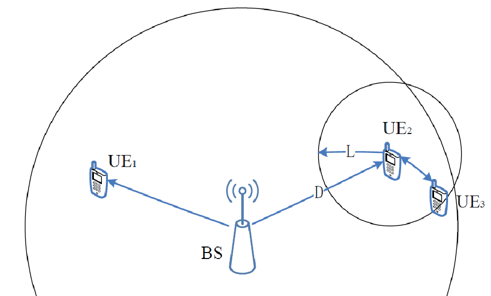
According to Fig. 1.1, three communicating users are in the system. UE2 and UE3 are in D2D mode, and UE1 is cellular user. We set the maximum distance between UE2 and UE3 is 25 meters. Actually, no more than 100 meters distance between them can be effective. The existing results only give a possible situation. Table 1.1 gives the main simulation parameters.
The wireless propagation is modeled according to WINNER II channel models, and D2D channel is based on office/indoor scenario while cellular channel is based on urban macrocell scenario. Table 1.2 gives path loss models. is the link distance in meters, and is the amount of walls penetrated in the link. , where is the centre frequency in Hz, m/s is the propagation velocity in free space, and and are the effective antenna heights at the BS and the MS, respectively. The effective antenna heights and are computed as follows: , m where and are the actual antenna heights, and the effective environment height in urban environments is assumed to be equal to 1.0 m. The LOS probability is given in Table 1.3.
| Parameter | Value |
|---|---|
| Cellular | Isolated cell,1-sector |
| System area | User devices are distributed within |
| a range of 500m from the BS | |
| Noise spectral density | -174dBm/Hz |
| System bandwidth | 5MHz |
| Noise figure | 5dB at BS/9dB at device |
| Antenna gains and patterns | BS:14dBi; Device: Omnidirectional 0dBi |
| Cluster radius | 5m,10m,15m,20m,25m |
| Transmit power | BS:46dBm; |
| Device: 24dBm (without power control) |
| Scenario | Path loss [dB] | Shadow fading [dB] |
|---|---|---|
| D2D (LOS) | 3 | |
| D2D | 4 | |
| (NLOS) | ||
| Cellular | 4 for | |
| (LOS) | 6 for , | |
| , | ||
| Cellular | 8 for , | |
| (NLOS) | , | |
| D2D user- | 7 | |
| Cellular user | ||
| Scenario | LOS probability |
|---|---|
| D2D | |
| Cellular |
Next, we investigate D2D and cellular SINR distribution with power control. The LTE uplink open loop fraction power control scheme (OFPC) is given as [20]
| (1.1) |
The parameters for the power control scheme are given in Table 1.4.
| Parameter | Value |
|---|---|
| 24dBm | |
| -78dBm | |
| 0.8 | |
| L | Path loss between two UEs in a pair. |
| M | 1 |
In this scenario, the interference between D2D and cellular users has been taken into account due to UL resource sharing. When the distance between D2D and co-channel cellular users is not larger than the maximum distance of D2D communication, the interference channel can be based on indoor/office scenario. But when co-channel interference comes from a farther location, D2D channel model is not suitable. According to WINNER II channel models, we choose indoor-to-outdoor/outdoor-to-indoor scenario to simulate long-distance interference channel.
Table 1.2 also gives the interference channel model. is the path loss of urban microcell scenario (see pp.44 in [19] for parameter detail), is the distance between the outdoor terminal and the point on the wall that is nearest to the indoor terminal, is the distance from the wall to the indoor terminal, is the angle between the outdoor path and the normal of the wall. For simplicity, we can assume so that in the simulation.


Consider a scenario of 19 cells, each of which is shown as Fig. 1.1. For simplicity, a model with one cellular user and one D2D pair is considered. Update the locations of three users in each simulation loop. Moreover, co-channel interference is taken into account. Neighbor cell interference is also from D2D, cellular users(UL), and BS(DL). Fig. 1.2 and Fig. 1.3 give the SINR distribution of D2D communication without power control (PC) mechanism in downlink (DL) and uplink (UL) period, respectively.
When D2D users share cellular DL resources without PC: D2D SINR is better when the pair is farther away from BS. Cellular (UE1) SINR is less sensitive to the location of D2D users. UE1 SINR is better than D2D SINR. When sharing DL resources, the interference to D2D is from BS. The position of the pair has direct influence on the strength of the interference. For cellular user, the strength of interference depends not only on the position of D2D users, but also on the position of cellular user. Since both are randomly distributed, the position of D2D pair does not significantly affect the results. UE transmit power is smaller than BS, thus interference from BS can be higher than that from D2D. As a result, D2D SINR is clearly worse than UE1.
When D2D users share cellular UL resources without PC: D2D SINR is almost unchanged as the distance from BS to the pair changes. BS SINR is better when D2D pair is farther away from BS. D2D SINR is better than BS SINR. In UL resource sharing, the strength of D2D interference depends not only on the position of D2D users, but also on the position of cellular user. Since both are randomly distributed, the position of D2D pair does not significantly affect the results. For BS, the interference is from D2D users. The position of the pair has direct influence on the strength of the interference. UE3 is 0 25m from UE2 and UE1 is 0 500m away from BS, which is likely to make D2D receive power larger than BS receive power.
Fig. 1.4 and Fig. 1.5 are the SINR distribution of D2D communication under PC in DL and UL period, respectively. When D2D users share cellular DL resources with PC: D2D SINR has decreased. UE1 SINR has increased. When D2D users share cellular UL resources with PC: D2D SINR has decreased. BS SINR has increased. Fig. 1.6 is the comparison of SINR distribution between D2D communication with and without PC. By PC, D2D SINR has decreased about 30dB. D2D SINR with PC gives smaller dynamic range.
OFPC scheme limits the transmit power of D2D users, which leads to D2D SINR degradation. Because D2D transmit power drops down, the interference to cellular user and BS decreases. Due to the path loss compensation in OFPC scheme, D2D SINR obtains a more concentrated distribution.
1.3 Mode Selection
In Device-to-Device (D2D) underlay communication system, one of the most challenging problems is to decide whether communicating devices should use cellular or direct communication mode. In D2D mode the data is directly transmitted to the receiver while cellular communication mode requires the source device transmit to the base station (BS) and then the destination device receives from the BS on downlink (DL). Here we consider three different mode selection criteria.
- 1.
Cellular: All devices are in cellular mode.
- 2.
Force D2D: D2D mode is selected always for all the communicating devices.
- 3.
PL D2D: D2D mode is selected if any of the path losses between source device and its serving BS, destination device and its serving BS, is greater than the path loss between a source and a destination in a pair.
Here, we give the results in the multi-cell scenario of D2D communication. Because it is closer to the practical applications. The single-cell scenario is similar to this case, and will not be repeated.


Consider a scenario of 19 cells with multiple users. The total number of users in the center cell is , in which 2000 users are communicating. At first, a communicating user is distributed uniformly in the cell. Another one follows a uniform distribution inside a region at most L from the first user, thus a link pair is formed. Accordingly, all the users should be located in the cell. Fig. 1.7, 1.8, 1.9, 1.10 show the SINR distribution of D2D communication under different mode with m, respectively. When the distance between D2D devices is small (L=5m): FORCE, PL criterion give the same capacity distribution, and CEL mode falls behind. As the maximum distance between D2D devices increases to 15m: The capacity is still better under FORCE, PL criterion, but it has decreased. PL mode gives higher capacity than FORCE mode does. The maximum distance between D2D devices increases to a larger value (L=35m): FORCE mode gives a large SINR dynamic range and more than users SINR is lower than that under CEL mode. PL mode is the best one. D2D devices are away from each other at most 45m: FORCE mode gives the worst capacity distribution. CEL and PL mode are similar.
As the maximum distance between users in a pair increases, the performance of direct communication degrades. There exists a threshold value of L for deciding whether to use D2D communication. PL mode is a method to solve the problem. Choose the better channel condition from cellular and D2D communication can obtain an optimal performance results.
1.4 Introduction to Game Theory in D2D Communication
Due to the interference caused by spectrum resource sharing between D2D and cellular users, resource management becomes a key issue to be settled. Game theory offers a set of mathematical tools to study the complex interactions among interdependent rational players and to predict their choices of strategies [21]. In recent years, game theory has emerged as a tool for the design of wireless communication networks. Therefore, we employ game theory on resource scheduling and interference avoidance in D2D communication. In this section, some necessary definitions are briefly introduced, and current researches on wireless communications based on game theory are also mentioned. Moreover, we give an overview of game theory method solving problems of D2D communication in this book.
The key elements of a game are the players, the actions, the payoffs (utilities) and the information, together known as the rule of the game. Players are the individuals making decisions, which can be denoted as a set . An action is a choice that player makes. An action profile is a set of all players’ actions. In an auction, players are the bidders and actions are the bids submitted by the bidders. Player ’s utility is a function of the action profile , and the utility describes how much gains the player gets from the game for each possible action profile. In the games, a player’s utility equals his value for the action profile minus his payment , i.e., . An important assumption of game theory is that all players are rational, i.e., they intend to choose actions to maximize their utilities. A player’s information can be characterized by an information set, which tells what kind of knowledge the player has at the decision instances. In order to maximize their utilities, the players would design their strategies, which are mappings from one player’s information sets to his actions.
A reasonable prediction of a game’s outcome is an equilibrium, where each player chooses a best strategy to maximize his utility. Among several available equilibrium concepts, we mainly put emphasis on the Nash Equilibrium (NE). In a static game, an NE is a strategy profile where no player can increase his utility by deviating unilaterally.
In the present researches, game theory including a large number of different game methods are used to analyze resource allocation problems, such as power and wireless spectrum allocations in communication networks [22], resource management in grids [23], and distributed resource coordination in mega-scale container terminal [24]. In [22], the authors proposed a sequential auction for sharing the wireless resource, which is managed by a spectrum broker that collects bids and allocates discrete resource units using a sequential second-price auction.
A combinatorial auction model for resource management was introduced in [23, 24]. The combinatorial auction-based resource allocation mechanism allows an agent (bidder) to place bids on combinations of resources, called “packages”, rather than just individual resource unit. Actually, the combinatorial auctions (CAs) have been employed in a variety of industries for, e.g., truckload transportation, airport arrival and departure slots, as well as wireless communication services. The benchmark environment of auction theory is the private value model, introduced by Vickrey (1961), in which one bidder has a value for each package of items and the value is not related to the private information of other bidders [25]. Much of work has not recognized that bidders care in complex ways about the items they compete. The CAs motivate bidders to fully express their preferences, which is an advantage in improving system efficiency and auction revenues. Up to that point, our interest is to apply the CA game in solving arbitrary D2D links reusing the same cellular frequency bands with the purpose of optimizing the system capacity.
However, it exists a series of problems and challenges in CAs, such as pricing and bidding rules, the winner determination problem (WDP) which, as mentioned in the literature, leads to the NP-hard allocation problem. Therefore, we focus on the evolution mechanisms named iterative combinatorial auctions (I-CAs) [26, 27]. In I-CAs, the bidders submit multiple bids iteratively, and the auctioneer computes provisional allocations and ask prices in each auction round.
In Chapter 3, we study an effective spectrum resource allocation for D2D communication as an underlay to further improve system efficiency based on the I-CA. The whole system consists of the BS, multiple cellular users that receive signals from the BS, and multiple D2D pairs that communicate with respective receivers using licensed spectrum resources. Considering that interference minimization is a key point and multiple D2D pairs sharing the same resources can bring large benefits on system capacity, we formulate the problem as a reverse I-CA game. That means, the resources as the bidders compete to obtain business, while D2D links as the goods or services wait to be sold. By this way, the packages of D2D pairs are auctioned off in each auction round. Furthermore, we investigate some important properties of the proposed resource allocation mechanism such as cheat-proof, convergence and price-monotonicity. We reduce the computational complexity and apply the scheme to WINNER II channel models [19] which contain a well-known indoor scenario. The simulation results show that the auction algorithm leads to a good performance on the system sum rate, and provides high system efficiency while has lower complexity than the exhaustive search allocation.
Prior works have considered little about time-domain scheduling of D2D communication. In Section 4.1, we study joint scheduling, power control and channel allocation for D2D communication using a game theoretic approach. Note that if cellular and D2D UEs are simply modeled as selfish players, the outcome is usually inefficient, since cellular UEs do not want to share the channels with D2D UEs. As D2D communication is an underlay to the primary cellular networks, the concept of the Stackelberg game is well suited for the system. The Stackelberg game is hierarchical, and has a leader and a follower. The leader acts first, and then the follower observes the leader’s behavior and decides his strategy. The Stackelberg game has been employed in cooperative networks [28] and cognitive radio networks [29, 30]. In our proposed Stackelberg game, the cellular UEs are viewed as leaders and the D2D UEs are followers. We group cellular and D2D UEs into leader-follower pairs. The leader charges some fees for the follower using the channel. We analyze the optimal price for the leader and the optimal power for the follower. The strategies lead to a Stackelberg equilibrium. Then, we propose a joint scheduling and resource allocation algorithm. The leader-follower pairs form a priority queue based on their utilities, and the system schedules the D2D UEs according to their orders in the queue.
The booming wireless services are drawing more energy from UE batteries. However, UEs are typically handheld equipments with limited battery lifetime. Users have to constantly charge their batteries. One major advantage of D2D communication is to decrease UE transmit power consumption, and thus, extend the battery lifetime. In Section 4.2, we further explore this issue. We consider the energy consumption of UEs includes transmission energy and circuit energy, and model the battery lifetime using the Peukert¡¯s law [31]. We formulate the problem as maximizing the battery lifetime of D2D UEs subject to a rate constraint. The problem is complicated to solve directly. Thus, we consider a game-theoretic approach, where D2D UEs are viewed as players. The players are self-interested, and they complete to maximize their own battery lifetime. We construct the resource allocation game and analyze the best response, Nash equilibrium and Pareto efficiency of the game. The players may create externality when they selfishly occupy radio resources, causing a decrease in the quality of cellular communications. Thus, we modify the game by adding pricing as penalty and propose the resource auction. Simulation results show that the proposed algorithm has good performances in battery lifetime.
Chapter 2 Physical-layer Techniques
The demand of high-speed data services to wireless bandwidths grows rapidly, which has promoted various technology development. D2D has been proposed to be an underlay to the cellular network aiming to improve spectrum efficiency and system sum rate. For its potential to resource reuse and system capacity improvement, D2D communication is considered to be a key feature of the next generation wireless network, and attracts much attention. But it is worth noting that D2D may cause undesirable interference to the primary cellular users due to the spectrum sharing. This chapter focuses on some physical-layer techniques for resource management and interference avoidance of D2D communication underlaying cellular networks.
A simple power control scheme for D2D communication is proposed in Section 2.1, and in Section 2.2, we investigate a joint beamforming and power control mechanism to avoid interference between cellular and D2D links as well as maximize system throughput.
2.1 Power Control
In this section, a threshold-based power control scheme for D2D links is proposed to improve the performance of D2D underlay systems. Both interference management and power saving are considered in this scheme.
2.1.1 Power Control Scheme
Fig. 2.1 gives the radio resource sharing of D2D and cellular links. We can see that the co-channel interference cannot be ignored. Uplink (UL) resource reuse has better performance on D2D channel rate and operability compared to downlink resource reuse. However, to efficiently sharing UL spectrum resource, it is necessary to mitigate the interference from D2D transmitter to the BS; moreover, saving power as much as possible while satisfying a reliable level of performance for D2D users will promote the system efficiency.

Fig. 2.2 shows the interference scenario of UL resource sharing. We can see that D2D transmitter UE1 causes interference to the BS, while cellular user UE3 causes interference to D2D receiver UE2. Existing work [1, 3, 11] propose some power control schemes for D2D transmissions. [1] employs the eNB to control the maximum transmit power of D2D transmitters which achieves the purpose of limiting the co-channel interference. In [3], D2D power is controlled by the eNB according to statistical results at the eNB. [11] proposes a greedy sum rate maximization optimization with full CSI assumption. However, these schemes do not consider the practical communication constraints and detailed mechanism design. The patent [32] adjusts D2D transmit power according to HARQ feedback from the eNB to cellular UE, which is unreliable in judging the interference status by HARQ monitoring.

The patent [33] takes the following scheme: the eNB makes measurements of interference from D2D transmitter to cellular link, computes appropriate backoff or boost values, and sends a power control command to D2D transmitter. Although this scheme control the interference relatively effectively, the quality of D2D link is not counted for the system, which may cause performance loss. Further, it needs centralized scheduling as the eNB should control both D2D and cellular communication for interference measurement, which leads to large system overhead. Based on the above, considering both cellular and D2D link performances, this section proposes a power control method which can be utilized with distributed scheduling under uplink resource sharing.
The key ideas of this scheme are as follows.
- 1.
The BS has no direct control on the D2D link but notifies an interference margin threshold to D2D transmitter.
- 2.
The BS feeds back the CSI of D2D transmitter UL channel (not needed for TDD system as the CSI can be obtained by channel symmetry).
- 3.
D2D transmit power is calculated by D2D transmitter itself with knowledge of the CSI and the interference margin threshold.
- 4.
D2D transmitter can freely decide whether to transmit according to allowed transmit power and D2D link status.
The key benefits of the above scheme: the system satisfies D2D link quality while guarantees cellular link away from destructive interference, which further improves system performance. In addition, the scheme has better scalability as distributed characteristics. It could both restrain interference and guarantee the feasibility of D2D connection.
A simplified process of signaling interactions is shown in Fig. 2.3, and Fig. 2.4 lists the implementation process of the proposed D2D power control.


2.1.2 Threshold Based Power Calculation
In this scheme, D2D transmitter can calculate the permitted transmit power bound according to the obtained CSI and the interference margin threshold. For the uplink resource sharing, we assume the minimum SINR at the BS is required for , and the interference margin threshold is represented as . Then, the corresponding SNR (without the co-channel interference) and SINR at the BS are expressed as
| (2.1) |
| (2.2) |
respectively. Here, and denote the transmit signal power of cellular and D2D user, respectively. and represent the path-loss and the channel gain between the BS and cellular user. and are the path-loss and the channel gain between D2D transmitter and the BS. is the AWGN noise power.
According to (2.1), the transmit power of cellular user satisfies
| (2.3) |
If the transmit power of cellular user takes the minimum value , (2.2) can be transformed into
| (2.4) |
Thus, on the premise of satisfying the interference margin , the maximum transmit power of D2D is .
We consider that the channel gain in the practical system may be estimated, then we have
| (2.5) |
Moreover, we consider the received power of D2D user , where and are the path-loss and the channel gain between D2D transmitter and receiver. Thus, we fine tune the transmit power as , and we obtain
| (2.6) |
where and are the channel gain estimation values.
For the performance of D2D links, it requires to satisfy the minimum SINR of receiver , i.e.,
| (2.7) |
where and represent the path-loss and the channel gain between cellular user and D2D receiver. So we have
| (2.8) |
Here, is the minimum transmit power to guarantee the performance of D2D links.
Next, we give some simulation results and related analysis. Power saving and energy efficiency are two sides that been investigated. We define the power saving as
| (2.9) |
where is the fixed transmit power of D2D users, is the transmit power of cellular users by LTE uplink open loop fraction power control scheme, and is the transmit power of D2D users by the proposed power control scheme while satisfying the constraints . That is, power saving factor represents the percentage of saving power by the power control scheme compared to the fixed power scheme. In the simulation, energy efficiency can be calculated by
| (2.10) |
Here, and denote the SINR at the BS and D2D receiver, respectively. The simulation parameters are listed in Table 2.1.
| Parameter | Value |
|---|---|
| Cellular | Isolated cell, 1-sector |
| System area | User device are distributed in a |
| hexagonal cell with 500m radius. | |
| Noise spectral density | -174dBm/Hz |
| Sub-carrier bandwidth | 15kHz |
| Noise figure | 5dB at BS/9dB at device |
| Antenna gains and patterns | BS: 14dBi |
| Device:Omnidirectional 0dBi | |
| Cluster radius | 150m |
| Minimum SINR | BS: 10dB |
| Device: 5dB | |
| Number of cellular users (channels) | 1/1:8 |
| Interference margin | 3dB |
| Transmit power bound | Max: 23dBm |
| Detecting signal power | 5dBm |
| Channel model | WINNER II |


Fig. 2.5 and Fig. 2.6 give the percentage of power saving and the distribution of energy efficiency under statistical channel estimation, respectively. The power control scheme saves about power than the fixed power 23dBm. Besides, the power control scheme statistically performs better than fixed power case in energy efficiency, and the performance is similar to the centralized scheme in the patent [33].
Fig. 2.7 Fig. 2.9 show the distribution of D2D, cellular and system throughput under statistical channel estimation. Because of the D2D power control, the throughput of D2D link is lower than that under the fixed maximum power 23dBm, but higher than that under the centralized PC scheme due to the D2D link performance guarantee. The sum throughput is also appreciable as excessive interference to cellular links is avoided.
This section has proposed a distributed threshold-based power control scheme that guarantees the feasibility of D2D connection, and at the same time limits cellular SINR degradation. The BS has no direct control on the D2D link but notifies an interference margin threshold to D2D transmitter, and the value can be tuned to meet corresponding SINR requirements. Power is calculated by D2D transmitter itself, which makes the operation flexible and convenient, improving the system efficiency.
2.2 Beamforming
Same frequency-time resources could be shared by cellular and D2D links to enhance the system capacity, but co-channel interference exists. During downlink (DL), D2D links receive more interference from the BS. Interference management is necessary to optimize the system performance. On one side, we hope to achieve a reliable level of performance for both cellular and D2D users. On the other side, to maximize the system throughput is our objective. In this section, we investigate a joint beamforming and power control method to reduce the interference and further improve the system performance.
2.2.1 Joint Beamforming and Power Control Scheme
In this scheme, we consider a single cell scenario, and only one cellular user and one D2D pair in the model. We assume that the BS is equipped with multiple antennas while UEs are respectively with a single antenna. Fig. 2.10 gives the system model, where the solid lines indicate the data transmissions and the dotted lines indicate the interference links. Moreover, we assume the channel responses are known by the BS, and the SINR minimum threshold of both cellular and D2D users are set by the BS.

Fig. 2.11 gives an example of beamforming with two antennas equipped at the BS. The channel response matrix can be expressed as
| (2.11) |
where , are data channel responses of cellular link, and , are interference channel responses of D2D link. The transmitted signal at the BS is obtained by
| (2.12) |
Here, is beamforming matrix, is power normalization matrix, and is data vector. Thus, the received signal at cellular user and D2D receiver can be jointly written as
| (2.13) |

In this model, the BS is the control center which conduct beamforming and power control at the same time.
The key ideas of this scheme are as follows.
- 1.
The BS carries out beamforming to avoid D2D receiving excessive interference from the BS.
- 2.
D2D receiver and cellular user feed back downlink CSI to the BS.
- 3.
The BS calculates transmit power to maximize system sum rate subjected to SINR threshold of both cellular and D2D links.
The key benefits of the above scheme: the system better adapts to D2D link quality in downlink resource sharing. In general, the scheme could guarantee the performance of both cellular and D2D links, and could maximize system throughput as centralized characteristics.
A simplified process of signaling interactions is shown in Fig. 2.12, and Fig. 2.13 lists the implementation process of the proposed joint beamforming and power control scheme.


2.2.2 Beamforming Matrix and Power Calculation
The BS calculates the beamforming matrix according to the CSI that cellular and D2D user feedback to it. Based on the system model in subsection 2.2.1, the received signal at cellular user and D2D receiver can be written as
| (2.14) |
| (2.15) |
respectively. Here, is the signal channel response of cellular user, and is the interference channel response of D2D receiver. is the beamforming matrix satisfying . and represent transmit signals from the BS and D2D transmitter, respectively. and denote transmit power from the BS and D2D transmitter, respectively. is thermal noise with variance . We employ maximizing SLNR as the beamforming criterion. That is,
| (2.16) |
Thus, the beamforming matrix can be obtained by
| (2.17) |
where is the channel response from the BS to users, and is a normalization factor so that .
In this scheme, our objective is to maximize the system sum rate which is expressed as
| (2.18) |
In addition, the D2D transmit power also need to satisfy the SINR threshold of both cellular and D2D links, i.e.,
| (2.19) |
| (2.20) |
where and are the SINR minimum threshold of cellular user and D2D receiver, respectively. Thus, we can summarize the objective function as
| (2.21) |
| (2.22) |
where is the maximum transmit power that UE supports.
Next, we give some simulation results and related analysis. Throughputs of cellular, D2D users and the whole system are our main performance metrics. And we compare some different interference management schemes on the system performance, including:
- 1.
Proposed PC & BF: joint beamforming and power control;
- 2.
No PC & BF: only beamforming is applied, and power is fixed;
- 3.
PC & no BF: only power control is applied;
- 4.
No PC & no BF: neither power control nor beamforming is applied.
The simulation parameters are listed in Table 2.2.
| Parameter | Value |
|---|---|
| Cellular | Isolated cell, 1-sector |
| System area | User devices are distributed in a |
| hexagonal cell with 600m radius. | |
| Noise spectral density | -174dBm/Hz |
| System bandwidth | 20MHz |
| Sub-carrier bandwidth | 15kHz |
| Sub-carrier number of each user | 64 |
| Cluster radius (D2D user scattering) | 50m |
| Minimum SINR | 5dB (both cellular and D2D) |
| Number of cellular users (channels) | 1 |
| Number of D2D pairs | 1/1:4 |
| Device transmit power upper bound | 23dBm |
| BS total transmit power | 46dBm |
| Channel Model | WINNER II |


Fig. 2.14 shows the system throughput distribution with different schemes. Obviously, joint beamforming and power control scheme makes the whole system performance better. Fig. 2.15 and Fig. 2.16 give the throughput distribution of D2D and cellular user. On one side, beamforming makes the performance of D2D communication better as SLNR criteria constrains the interference from the BS to D2D receiver. On the other side, power control makes the performance of cellular communication better as it limits the interference from D2D to cellular user.
For multiple D2D pairs, we consider the objective function the same as that of single pair for simplicity. Fig. 2.17 is the result of the system throughput with different number of D2D pairs. We can see that the proposed scheme gives the optimal performance.
Fig. 2.18 gives the system throughput with different cellular radius. When the radius is small, beamforming prevents interference from BS to D2D effectively which makes the performance gain obvious. When the radius increases, the received signal power of cellular user decreases. Thus, power control becomes more important to prevent interference from D2D.
Fig. 2.19 shows the throughput of D2D user with different cellular radius. We find that power control does not bring strong fading to D2D communication. In fact, power control includes the mechanism that guarantees SINR of D2D being above the threshold, and the objective function of power control is the system throughput. We focus on the top two lines, and find the gap between the proposed scheme and the other one is comparably obvious when the cellular radius is small. Because cellular communication is dominant when the radius is small, system throughput would get profit from D2D power reducing. Thus, fading of D2D link becomes obvious.
This section has proposed a joint beamforming and power control scheme that aims to maximize the system sum rate while guarantees the performance of both cellular and D2D connections. The BS sets SINR threshold for D2D and cellular links, and the value can be tuned to meet corresponding performance requirements. The BS carries out beamforming to avoid D2D from excessive interference. D2D transmit power is calculated by the BS based on maximizing the system sum rate. Also, the BS decides whether the calculated D2D transmit power available according to SINR threshold of cellular and D2D links.
Chapter 3 Radio Resource Management
An innovative resource allocation scheme is proposed to improve the performance of mobile peer-to-peer, i.e., device-to-device (D2D), communications as an underlay in the downlink (DL) cellular networks. To optimize the system sum rate over the resource sharing of both D2D and cellular modes, we introduce a reverse iterative combinatorial auction as the allocation mechanism. In the auction, all the spectrum resources are considered as a set of resource units, which as bidders compete to obtain business while the packages of the D2D pairs are auctioned off as goods in each auction round. We first formulate the valuation of each resource unit, as a basis of the proposed auction. And then a detailed non-monotonic descending price auction algorithm is explained depending on the utility function that accounts for the channel gain from D2D and the costs for the system. Further, we prove that the proposed auction-based scheme is cheat-proof, and converges in a finite number of iteration rounds. We explain non-monotonicity in the price update process and show lower complexity compared to a traditional combinatorial allocation. The simulation results demonstrate that the algorithm efficiently leads to a good performance on the system sum rate.
3.1 Basics of Model and Auction Mechanism
In this section, we introduce the system model for D2D underlay communication. The scenario of multiple D2D and cellular users is first described, and then, the expression of system sum rate is given.
1) Scenario Description
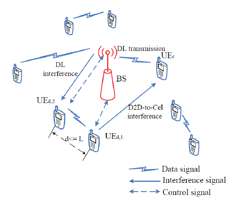
A model of a single cell with multiple users is considered. As shown in Fig. 3.1, UEs with data signals between each other are in the D2D communication mode while UEs that transmit data signals with the BS keep in the traditional cellular mode. Each user is equipped with a single omnidirectional antenna. The locations of cellular users and D2D pairs are randomly set and traversing the whole cell. Without loss of generality, we employ the uniform distribution to describe the user locations which is proposed for system simulation in [34]. Notice that from stochastic geometry with for Poisson distributions, the users are uniformly located as well if the number of users is known [35]. For simplicity and clarity, we illustrate co-channel interference scenario involving three UEs (UEc, UEd,1 and UEd,2), and omit the interference and control signal signs among others. UEc is a traditional cellular user that is distributed uniformly in the cell. UEd,1 and UEd,2 are close enough to satisfy the distance constraints of D2D communication, and at the same time they also have communicating demands. One member of the D2D pair UEd,1 is distributed uniformly in the cell, and the position of the other member UEd,2 follows a uniform distribution inside a region at most from UEd,1.
The existing researches [17, 18] confirm that with power control or resource scheduling mechanism, the inter-cell interference can be managed efficiently. Therefore, we place an emphasis on the intra-cell interference, which is due to resource sharing of D2D and cellular communication. Generally speaking, the session setup of D2D communication requires the following steps [1]:
- 1.
A request of communicating is initiated by one UE pair.
- 2.
The system detects traffic originating from and destined to the UE in the same subnet.
- 3.
If the traffic fulfills a certain criterion (e.g., data rate), the system considers the traffic as potential D2D traffic.
- 4.
The BS checks if D2D communication offers higher throughput.
- 5.
If both UEs are D2D capable and D2D mode offers higher throughput, the BS may set up a D2D bearer.
The cross-layer processes of resource control can be contained in the above steps, and be generally summarized as: the transmitters (both cellular and D2D users) send detecting signals. Then CSI would be obtained by corresponding receivers and be feedback to the control center (e.g. the BS). The power control and spectrum allocation are conducted based on certain principles. Finally, the BS sends control signals to users according to allocation results.
Even if the D2D connection setup is successful, the BS still maintain detecting if UE should be back to the cellular communication mode. Furthermore, the BS maintains the radio resource control for both cellular and D2D communication. Based on these communication features, we mainly focus on assigning cellular resources to D2D communication.
Here, we consider a scenario of sharing downlink (DL) resource of the cellular network as shown in Fig. 3.1. We assume UEd,1 is the transmitter of the D2D pair sharing the same sub-channel with the BS, and thus, UEd,2 as the D2D receiver receives interference from the BS. Also, the cellular receiver UEc is exposed to interference from UEd,1. In addition, the D2D users feed back the CSI to the BS, whereas the BS transmits control signals to the D2D pair, in the way that the system achieves D2D power control and resource allocation.
During the DL period of the cellular system, both cellular and D2D users receive interference as they share the same sub-channels. Here, we assume that any cellular user’s resource blocks (RBs) can be shared with multiple D2D pairs and each pair can use more than one user’s RBs for transmitting. We assume the numbers of cellular users and D2D pairs in the model are and , respectively. During the DL period, the BS transmits signal to the -th () cellular user, and the -th () D2D pair uses the same spectrum resources transmitting signal . The received signals at UE and D2D receiver are written as
| (3.1) |
| (3.2) |
where , and are the transmit power of BS, D2D transmitter , , respectively. is the channel response of the link that is from equipments to . and are the additive white Gaussian noise (AWGN) at the receivers with one-sided power spectral density (PSD) . represents the presence of interference satisfying when RBs of UE are assigned to UE , otherwise . As a cellular user can share resources with multiple D2D pairs, it also satisfies . Similarly, represents the presence of interference between D2D pairs and .
The channel is modeled as the Rayleigh fading channel, and thus, the channel response follows the independent identical complex Gaussian distribution. In addition, the free space propagation path-loss model, , is used where and represent signal power measured at and away from the transmitter, respectively. is the path-loss exponent. Hence, the received power of each link can be expressed as
| (3.3) |
where and are the received power and the distance of the link, respectively. represents the transmit power of equipment and is the complex Gaussian channel coefficient that obeys the distribution . And we simplify the received power at equals the transmit power.
2) System Sum Rate
For the purpose of maximizing the network capacity, the signal to interference plus noise ratio (SINR) should be considered as an important indicator. The SINR of user is
| (3.4) |
where denotes the interference signal power received by user , and accounts for the terminal noise at the receiver.
Determined by the Shannon capacity formula, we can calculate the channel rate corresponding to the SINR of cellular and D2D users. As cellular users suffer interference from D2D communicating that sharing the same spectrum resource, the interference power of cellular user is
| (3.5) |
While the interference of D2D receiver is from both BS and D2D users that are assigned the same resources to, the interference power of user can be expressed as
| (3.6) |
Based on (3.4), (3.5), and (3.6), we can obtain the channel rate of cellular user and D2D receiver as
| (3.7) |
| (3.8) |
respectively. Here, . So represents the interference from the other D2D pairs that share spectrum resources with pair .
The DL system sum rate can be defined as
| (3.9) |
In the next subsection, we formulate the problem of designing for each D2D pair as an optimization issue of maximizing .
In this subsection, we introduce two concepts: valuation model and utility function, which are bases of the auction mechanism. Also, some definitions are given.
3) Valuation Model
As D2D communication shares the same spectrum resources with cellular communication at the same time slot, the co-channel interference should be limited as much as possible to optimize the system performance. The radio signals experience different degrees of fading, and thus, the amount of interference depends on transmit power and spatial distances. Accordingly, we focus on assigning appropriate resource blocks (RBs) occupied by cellular users to D2D pairs in order to minimize interference to achieve a higher system sum rate. Next, we formulate the relation between the allocation result and the rate of the shared channel. The relation can be defined as a value function whose target value is the channel rate.
We define as a package of variables representing the index of D2D pairs that share the same resources. We assume the total pairs can form such packages. Thus, if the members of the -th () D2D user package share resources with cellular user , the channel rates of UE and D2D pair () can be written as
| (3.10) |
| (3.11) |
respectively. The rate of the operating channel shared by UE and D2D pairs is
| (3.12) |
According to (3.10) (3.12), when assigning resources of UE to the -th package of D2D pairs, the channel rate is given by
| (3.13) |
In the proposed reverse I-CA mechanism, we consider spectrum resources occupied by cellular user as one of the bidders who submit bids to compete for the packages of D2D pairs, in order to maximize the channel rate. It is obvious that there would be a gain of channel rate owing to D2D communicating as long as the contribution to data signals from D2D is larger than that to interference signals. Considering the constraint of a positive value, we define the performance gain as
| (3.14) |
which is the private valuation of bidder for the package of D2D pairs . Here, denotes the channel rate of UE without co-channel interference and is obtained by
| (3.15) |
Thus, we have the following definition:
Definition 1
A valuation model is a set of the private valuations of all bidders for all packages ().
4) Utility Function
In the auction, the cellular resource denoted by obtains a gain by getting a package of D2D communications. However, there exists some cost such as control signals transmission and information feedback during the access process. We define the cost as a pay price.
Definition 2
The price to be payed by the bidder for the package is called pay price denoted by . The unit price of item (, ) can be denoted by .
Here, we consider linear anonymous prices [26], which means the prices are linear if the price of a package is equal to the sum of the prices of its items, and the prices are anonymous if the prices of the same package for different bidders are equal. Thus, we have
| (3.16) |
Therefore, the payment of a bidder is determined by the unit price and the size of bidding package .
Definition 3
Bidder utility, or named bidder payoff expresses satisfaction of bidder getting package . The bidder utility can be defined as
| (3.17) |
Based on (3.14), (3.16), (3.17), in (3.13) and in (3.15), we can obtain the utility of bidder as
| (3.18) |
In order to describe the allocation outcome intuitively, we give the definition below.
Definition 4
The result of the auction is a spectrum allocation denoted by , which allocates a corresponding package to each bidder. And the allocated packages may not intersect ().
We consider a set of binary variables to redefine the allocation as
| (3.19) |
According to the literature, two most popular bidding languages are exclusive-OR (XOR), which allows a bidder to submit multiple bids but at most one of the bids can win, and additive-OR (OR), which allows one to submit multiple bids and any non-intersecting combination of the bids can win. We consider the XOR bidding language. Thus, (3.19) satisfies and for . If given an allocation , the total bidder utility of all bidders can be denoted as . Furthermore, the auctioneer revenue is denoted as , which is usually considered to be the auctioneer’s gain.
3.2 Resource Allocation Algorithm Based on Reverse Iterative Combinatorial Auction
In this section, we formulate the resource allocation for D2D communication as a reverse I-CA game. First, we introduce some concepts of the I-CA games. Then, we investigate details of the allocation process.
1) Reverse Iterative Combinatorial Auction Game
As mentioned before, we assume the total spectrum resources are divided into units with each one already providing communication service to one cellular user. By the auction game, the spectrum units are assigned to user packages , with each package consisting of at least one D2D pair. In other words, the spectrum units compete to obtain D2D communication for improving the channel rate.
During an I-CA game, the auctioneer announces an initial price for each item, and then, the bidders submit to the auctioneer their bids at the current price. As long as the demand exceeds the supply, or on the contrary that the supply exceeds the demand, the auctioneer updates (raises or reduces) the corresponding price and the auction goes to the next round.
Obviously, it can be shown that the overall gain, which includes the total gain of the auctioneer and all bidders does not depend on the pay price, but equals to the sum of the allocated packages’ valuations, i.e.,
| (3.20) |
As our original intention, we employ the I-CA to obtain an efficient allocation for spectrum resources.
Definition 5
An efficient allocation denoted by is an allocation that maximizes the overall gain.
Given the private bidder valuations for all possible packages in (3.14), an efficient allocation can be obtained by solving the combinatorial allocation problem (CAP).
Definition 6
The Combinatorial Allocation Problem (CAP), also sometimes referred as Winner Determination Problem (WDP), leads to an efficient allocation by maximizing the overall gain: , where denotes the set of all possible allocations.
An integer linear program using the binary decision variables is formulated for the CAP as
| (3.21) | ||||
The objective function maximizes the overall gain, and the constraints guarantee: 1) at most one package can be allocated to each bidder; 2) each item cannot be sold more than once.
In fact, there might be multiple optimal solutions of the CAP with the same objective function. From the auctioneer’s point of view, tie-breaking rules are needed to determine which of the optimal solutions is selected. In a real auction, the auctioneer does not know the private valuations of the bidders, neither can it solve the NP-hard problem. To solve the CAP, the auctioneer selects the winners on the basis of the submitted bids in each round. Therefore, in case of the XOR bidding language, the WDP formulation is similar to the CAP and the only difference is the objective function
| (3.22) |
where represents the pay price of bidder for package in round .
Based on Definition 5, the overcome of a CA is not always efficient. Here, we employ allocating efficiency as a primary measure to benchmark auctions.
Definition 7
Allocating efficiency in CAs can be expressed as the ratio of the overall gain of the final allocation to that of an efficient allocation [26]
| (3.23) |
which has .
2) Algorithm for Resource Allocation
In this subsection, the details of the allocation scheme based on reverse I-CA are introduced. We has modeled the D2D resource allocation problem as a reverse I-CA game and gave the valuation model, utility function and other important concepts. Many I-CA designs, especially for the centralized I-CA design, are based on ask prices. The price-based I-CA designs differ by the pricing scheme and price update rules. In the proposed algorithm, linear prices are used as mentioned in Section 3.1 for they are easy to understand for bidders and convenient to communicate in each auction round. Because of the interference from D2D links, cellular channels should guarantee the performance of cellular system before allowing the D2D access. Hence, we consider a descending price criterion in the algorithm. Prices update by a greedy mode that once a bidder submits a bid for items or packages the corresponding prices are fixed, otherwise the prices are decreased.
At the beginning of the allocation, the BS collects the location information of all the D2D pairs. In addition, the round index , the initial ask price for each item (D2D pair) , and the fixed price reduction are set up. When the initial prices are announced to all the bidders (i.e. spectrum resources occupied by cellular UEs), each bidder submits bids, which consist of its desired packages and the corresponding pay prices. Jump bidding where bidders are allowed to bid higher than the prices, is not allowed in our scheme, thus bidders always bid at the current prices. According to the CAP proposed in Definition 6 and the analysis about the WDP, we simplify the problem of maximizing the overall gain as a process of collecting the highest pay price. As a result, bidder bids for package as long as . Combining (3.16) and (3.17), we have
| (3.24) |
where the round index . In this case, let denote the submitted bid at the end of round , and denotes all the bids. When (3.24) is not satisfied, bid . If satisfies , it reveals that the supply exceeds the demand. Then, the BS sets , where is the over-supplied item, and the auction moves on to the next round.
In a normal case, as long as the price of a package decreases below a bidder’s valuation for that package, the bidder submits a bid for it. The BS allocates the package to the bidder, and fixes the corresponding prices of items. At the same time, constrained by the XOR bidding language, the bidder is not allowed to participate the following auction rounds. As the asking prices decrease discretely every round, it may exist a situation that more than one bidders bid for packages containing the same items simultaneously. The BS detects the bids of all the bidders: 1) it exists (); 2) it exists , () satisfying . If either of the above conditions is satisfied, the overall demand exceeds supply for at least one item. Then, the BS sets a fine tuning where is the temporary over-demanded item, and can be set by where is an integer factor that affects the convergence rate. The allocation can be determined by multiple iterations.
The auction continues until all the D2D links are auctioned off or every channel wins a package. Our algorithm is detailed in Table 3.1.
| Initial State: The BS collects the location information of all D2D pairs. The valuation of the -th resource unit for package is , which is given by (3.14). The round index , and the initial price , the fixed price reduction are set up. |
| Resource Allocation Algorithm: 1. Bidder submits bids depending on its utility. bidder bids for package as long as , which is represented by (3.24). If , bidder submits . 2. If satisfies , the BS sets , where is the over-supplied item, and the auction moves on to the next round. Return to step 1. 3. The BS detects the bids of all the bidders: 1) it exists (); 2) it exists , () satisfying . 4. If neither of the conditions in step 3 is satisfied, go to step 5. Otherwise, the overall demand exceeds supply for at least one item. The BS sets , and can be set by where is an integer factor. Return to step 1. 5. The allocation can be determined by repeating the above steps. The auction continues until all D2D links are auctioned off or every cellular channel wins a package. |
3.3 Analysis of the Auction-Based Resource Allocation Algorithm
In this section, we investigate the important properties of the proposed auction-based resource allocation mechanism.
1) Cheat-Proof
As the general definition, cheat-proof means that reporting the true demand in each auction round is a best response for each bidder.
Proposition 1
The resource allocation algorithm based on the reverse I-CA is cheat-proof.
Proof 1
From (3.18), we can get that the utility of bidder depends on the valuation of the package it bids and unit prices of the items. In details, it is the interference (between cellular and D2D communications) that mainly affects the utility. As the expression is extremely complex to resolve, we consider the case that only one item constitutes the package without loss of generality. The utility of bidder can be rewritten as
| (3.25) |
and the differential expressions of the utility with respect to and are
| (3.26) |
| (3.27) |
respectively. Accordingly, utility is a monotonically decreasing function with respect to both and . Thus, the optimal strategy is to bid the D2D link that has a lower channel gain with the cellular transmitter and receiver.
In a descending price auction, items are always too expensive to afford at the beginning. With the number of iterations increasing, the prices of items drop off. Given a package in round , bidder has the right to submit bid or . Given that all the other bidders submit their true demands according to (3.24), we consider the strategy of bidder in two cases: 1) if bids when its true valuation for satisfies , it will quit this round and lose the package which maximizes its channel rate; 2) if bids when its true valuation for satisfies and finally wins the package, it will obviously get a negative surplus that is unwanted.
From the above analysis, we can conclude that the optimal strategy for cellular channel is to submit its true demand in each round, or it will get a loss in its utility as a result of any deceiving. That is, the proposed resource allocation algorithm is cheat-proof.
2) Convergence
In this subsection, we prove that the proposed algorithm has the convergence property.
Proposition 2
The resource allocation algorithm based on the reverse I-CA has the convergence property that the number of the iterations is finite.
Proof 2
According to Theorem 1, all the bidders submit their true demands in each auction round, in order to obtain the utility from winning. From (3.18), we can derive
| (3.28) |
where denotes the utility of bidder in round . According to the algorithm, we have that bidder will get zero utility with no bid if , and have an opportunity to win a positive utility with bid if . Therefore, in the beginning, bidder plays a waiting game, and once , it will bid for . As long as it is the only one that submits a bid, it will get the package. With a sufficiently large and , we can finally get . Similarly, if more than one bidders bid for the same item, we can have an allocation by ascending price process with the step . Subjected to in (3.21), the package can not be sold once more. Thus, for a finite number of packages , the number of iterations is finite. That is, the proposed scheme would reach convergence.
In addition, the value of the price step has a direct impact on the speed of convergence of the proposed scheme. The scheme converges fast when is large, while it converges slowly when is small. The fine tuning also has the same nature, but less impact on convergence.
3) Price Monotonicity
In an I-CA game, the price updates through several ways, i.e., monotonically increasing, monotonically decreasing and non-monotonic modes. Here, we focus on the price non-monotonicity in the proposed reverse I-CA algorithm.
Proposition 3
In the proposed descending price auction, the raising item prices in a round may be necessary to reflect the competitive situation. Moreover, it brings efficiency improvement.
Proof 3
From the algorithm proposed in Table 3.1, there exists a situation that more than one bidders submit bids for the same package or different packages with intersection when prices are reduced to some certain values. But auctions do not allow one item being obtained by multiple bidders as the second constraint in (3.21) shows. In this situation, raising the corresponding prices by a fine tuning makes bidders to reinspect their utility functions. Once a bidder finds its utility less than zero, it quits from the competition. By a finite number of iterations, the winner converges to one bidder. Since the ascending price process maximizes the auctioneer revenue as shown in (3.22), the allocation has higher efficiency than a random allocation in that situation.
4) Complexity
As mentioned before, a traditional CAP in fact is an NP-hard problem, the normal solution of which is the centralized exhaustive search. We set that the number of items to be allocated is , and the number of bidders is . For an exhaustive optimal algorithm, an item can be allocated with possible results. Thus, all the items are allocated with possible results. The complexity of the algorithm can be denoted by . In the proposed reverse I-CA scheme, bidders reveal their entire utility function, i.e., they calculate valuations for all possible packages, the number of which is . If the total number of iterations is , the complexity of the auction-based scheme is . From the proposed algorithm, we have (The fine tuning has a small impact on the result and can be omitted here). So the worst case is . It is obvious that for sufficient large values of and , general values of and , a much lower complexity is obtained by using the proposed reverse I-CA scheme. That is, . If we constrain the number of D2D pairs sharing the same channel to one, the complexity would be further reduced to . And the performance of this reduced scheme is included in the simulation in Section 3.4.
5) Overhead
In D2D underlay system, the BS is still the control center of resource allocation, and the global CSI should indeed be available at the BS for the proposed scheme. In addition to the CSI detection, feedback, and the control signaling transmission, the reverse I-CA scheme does not need additional signaling overhead compared to existing resource scheduling schemes such as maximum carrier to interference (Max C/I) and proportional fair (PF), which also need the global CSI to optimize the system performance. The difference is that the reverse I-CA scheme requires more complicated CSI due to the interference between D2D and cellular network.
At the beginning of the allocation, the transmitters need to send some packets containing detection signals. Then, the obtained CSI at each terminal (D2D or cellular receiver) would be feedback to the BS. After that, iteration process would be conducted at the BS, and no signaling needs to be exchanged among the network nodes until the control signals forwarding.
Methods, such as CSI feedback compression and signal flooding, would help reduce the overhead. In addition, the future work on D2D communication could consider some mechanism that limit the number of D2D pairs sharing the same channel by, e.g. distance constraint, which would obviously help reduce the overhead. But for this chapter, the target is to obtain the nearest-optimal solution, wherefore we do not consider the simplification.
3.4 Performance Results and Discussions
The main simulation parameters are listed in Table 3.2. As shown in Fig. 3.1, simulations are carried out in a single cell. Both path-loss model and shadow fading are considered for cellular and D2D links. The wireless propagation is modeled according to WINNER II channel models [19], and D2D channel is based on office/indoor scenario while cellular channel is based on the urban microcell scenario.
| Parameter | Value |
|---|---|
| Cellular layout | Isolated cell, 1-sector |
| System area | The radius of the cell is 500 m |
| Noise spectral density | -174 dBm/Hz |
| Sub-carrier bandwidth | 15 kHz |
| Noise figure | 9 dB at device |
| Antenna gains | BS: 14 dBi; Device: 0 dBi |
| The maximum distance of D2D | 5 m |
| Transmit power | BS: 46 dBm; Device: 23 dBm |
1) System Sum Rate
The system sum rate with different numbers of D2D pairs and different numbers of resource units using the proposed auction algorithm is illustrated in Fig. 3.2 Fig. 3.4. The sum rate can be obtained from (3.9).
From Fig. 3.2 and Fig. 3.4, we can see that the system sum rate goes up with both the number of D2D pairs and the number of resource units increasing. On one side, when the amount of resources is fixed, more D2D users contribute to a higher system sum rate. On the other side, as the amount of resource increases, the probability of resources with less interference to D2D links being assigned to them enhances, which can lead to the increased sum rate. This phenomenon is similar to the effect of multiuser diversity. Definitely, cellular users also contributes to the performance.
From another perspective, Fig. 3.2 Fig. 3.4 shows the system sum rate for different allocation algorithms. The curve marked exhaustive optimal is simulated by the exhaustive search way, which guarantees a top bound of the system sum rate. The curve marked reduced R-I-CA is the result of a reduced reverse I-CA scheme, in which the number of D2D pairs sharing the same cellular resources is constrained to one.


The curve marked R-I-CA represents the performance of the proposed reverse I-CA algorithm, and the last one is the simulation result using random allocation of spectrum resources. Firstly, we can see that the proposed auction algorithm is relatively much superior to the random allocation. Secondly, the optimal allocation results in the highest system sum rate, but the superiority compared to R-I-CA is quite small, especially when the number of cellular resource units increases as Fig. 3.4 shows. Moreover, we find that the performance of reduced R-I-CA approximates to that of R-I-CA scheme in case of 8 resource units, but differs obviously in case of 2 resource units shown in Fig. 3.3. The reason for this phenomenon is that the constraint of the reduced R-I-CA limits D2D pairs accessing to the network when the number of resources units is less than that of D2D pairs, thus a large capacity loss products.

2) System Efficiency
We define the system efficiency as , where represents the exhaustive optimal sum rate. Fig. 3.5 shows the system efficiency with different numbers of D2D pairs and different numbers of resource units. The simulation result indicates that the proposed algorithm provides high (the lowest value of is around 0.7) system efficiency. Moreover, the efficiency is stable over different parameters of users and resources.
As to the point of efficiency value being about 0.7, the number of resource units and the number of D2D pairs are both small. The linear price rule limits bidders to bid the maximal valuation packages, but to bid the packages having maximal average unit valuation. For this reason, the efficiency decreases slightly.
As to other points, the efficiency is stable above 0.9, which reflects a small performance gap between the proposed algorithm and the exhaustive search scheme. In fact, the descending price rule determines the bidder that has the highest bid on current items would win the corresponding package, which maximizes the current overall gain. However, the gap cannot be avoided as the algorithm essentially follows a local, or an approximate global optimum principle.
3) Price Monotonicity
Fig. 3.6 shows an example of the price non-monotonicity in the reverse I-CA scheme. The four curves represent unit price of four D2D pairs. As the enlarged detail shows, the unit price of D2D pair has an ascending process during the auction. As the step is much less than descending step , the phenomenon of ascending price is hard to pick out. When the items have been sold out, their prices are fixed to the selling value. And from the figure, we can find that the D2D pair is the last one to be sold.

In this chapter, we have investigated how to reduce the effects of interference between D2D and cellular users, in order to improve the system sum rate for a D2D underlay network. We have proposed the reverse iterative combinatorial auction as the mechanism to allocate the spectrum resources for D2D communications with multiple user pairs. We have formulated the valuation of each D2D pair for each resource unit, and then explained a detailed auction algorithm depending on the utility function. A non-monotonic descending price iteration process has been modeled and analyzed to be cheat-proof, converge in a finite number of rounds, and has low complexity. The simulation results show that the system sum rate goes up with both the number of D2D pairs and the number of resource units increasing. The proposed auction algorithm is much superior to the random allocation, and provides high system efficiency, which is stable over different parameters of users and resources.
Chapter 4 Cross-layer Optimization
D2D communication as an underlay to cellular networks brings significant benefits to system throughput and energy efficiency. However, as D2D UEs can cause interference to cellular UEs, the scheduling and allocation of channel resources and power to D2D communication need elaborate coordination. Thus, cross-layer optimization is considered in this chapter. In Section 4.1, both system throughput and fairness are taken into account. A joint time-domain scheduling and spectrum allocation scheme is studied. Based on the concept of UE’s battery lifetime, we propose an auction-based algorithm for power and channel resource allocation of D2D communication in Section 4.2.
4.1 Time-Domain Scheduling
In this section, we propose a joint scheduling and resource allocation scheme to improve the performance of D2D communication. We take network throughput and UEs’ fairness into account by performing interference management. Specifically, we develop a Stackelberg game framework in which we group a cellular UE and a D2D UE to form a leader-follower pair. The cellular user is the leader, and the D2D UE is the follower who buys channel resources from the leader. We analyze the equilibrium of the game, and propose an algorithm for joint scheduling and resource allocation. Finally, we perform computer simulations to study the performance of the proposed algorithm.
4.1.1 Model Assumptions
We still consider a single cell scenario with multiple UEs and one eNB located at the center of the cell. Both the UEs and the eNB are equipped with a single omni-directional antenna. The system includes two types of UEs, D2D UEs and cellular UEs. The D2D UEs are in pairs, each consisting of one transmitter and one receiver. We consider a dense D2D environment, where the number of cellular UEs and D2D UEs is and , respectively. The set of cellular UEs and D2D pairs is and , respectively. There are orthogonal channels, which is occupied by the corresponding cellular UEs. The channels allocated to the cellular UEs are fixed, and D2D communications share the channels with cellular UEs. One channel is only allowed to be used by one cellular UE and one D2D UE. In LTE, scheduling takes place every transmission time interval (TTI) [36], which consists of two time slots. Channels are allocated among D2D UEs according to their priority. During each TTI, D2D pairs are selected to share the channels with the cellular UEs while other D2D UEs wait for transmission.

A scenario of uplink resource sharing is illustrated in Fig. 4.1, which includes one cellular UE (UE1) and two D2D pairs (UE2 and UE3, UE4 and UE5). UE2 and UE4 are transmitters while UE3 and UE5 are receivers. The two D2D UEs in a pair are close enough to satisfy the maximum distance constraint of D2D communication, in order to guarantee the quality of D2D services. D2D pair 1 is selected to share the channel resource with UE1 whereas D2D pair 2 cannot transmit. During the uplink period of the cellular network, UE1 transmits data to the eNB, while the eNB suffers interference from UE2. Also, the D2D pair 1 is in communication while UE3 are exposed to interference from UE1.
During the downlink period, the cellular UE receives data from the eNB and interference from D2D transmitter sharing the same channel. The D2D receivers suffer interference from the eNB. The transmit power of eNB is too large, causing serious interference to the D2D UEs, so it is hard to guarantee the quality of D2D services. Therefore, we focus on the uplink frame of the network.
We define a set of binary variables to denote the current D2D pair in communication. if the -th D2D pair is selected to use channel ; and otherwise. Based on the analysis above, during the uplink period, the -th cellular UE transmits to the eNB, and the -th D2D transmitter transmits . The received signals at the eNB and D2D receiver are written as
| (4.1) |
| (4.2) |
where and is the transmit power of the -th cellular UE and the -th D2D transmitter, respectively. denotes the channel gain between the -th cellular UE and the -th D2D receiver. denotes the channel gain between the -th D2D transmitter and the -th D2D receiver, which are in a pair. is the channel gain between cellular UE and the eNB, and is the channel gain between D2D transmitter and the eNB. and is the additive white Gaussian noise (AWGN). Without loss of generality, we assume all UEs observe the same noise power .
The received SINR at the -th D2D receiver can be expressed as
| (4.3) |
The SINR at the eNB corresponding to cellular UE is
| (4.4) |
The channel rate of UEs is obtained by
| (4.5) |
4.1.2 Stackelberg Game
As D2D communication takes place underlaying the primary cellular network, we focus on the power control and scheduling of the D2D UEs, while the transmit power and channel of the cellular UE are assumed to be fixed. D2D communication can utilize the proximity between UEs to improve the throughput performance of the system. In the meanwhile, the interference from D2D network to the cellular network should be limited. Thus, the transmit power of the D2D UEs should be properly controlled. Another goal is to guarantee the fairness among D2D UEs when scheduling.
Interactions among the selfish cellular and D2D UEs sharing a channel can be modeled as a non-cooperative game using the game theory framework. When the players choose their strategies independently without any coordination, it usually leads to an inefficient outcome. If we simply model the D2D scenario as a noncooperative game, D2D UEs will choose to use the maximum transmit power to maximize their own payoffs regardless of other players, whereas cellular UEs will choose not to share the channel resources with D2D UEs. This is an inefficient outcome, as the interference is too serious or D2D cannot get access into the network.
Therefore, we employ the Stackelberg game to coordinate the scheduling, in which the cellular UEs are the leaders and the D2D UEs are the followers. We focus on the behavior of a one-leader one-follower pair. The leader owns the channel resource and it can charge the D2D UE some fees for using the channels. The fees are fictitious money to coordinate the system. Thus, the cellular UE has an incentive to share the channel with the D2D UE if it is profitable, and the leader has the right to decide the price. For the D2D UE, under the charging price, it can choose the optimal power to maximize its payoff. In this way, an equilibrium can be reached.
1) Utility Functions
We analyze the behavior of a one-leader one-follower pair, which includes cellular UE as the leader, and D2D pair as the follower. The utility of the leader can be defined as its own throughput performance plus the gain it earns from the follower. The fee should be decided according to the leader’s own consideration. Thus, we set the fee proportional to the interference the leader observe. The utility function of the leader can be expressed as
| (4.6) |
where is the charging price (). is a scale factor to denote the ratio of the leader’s gain and the follower’s payment (). is a key parameter to influence the outcome of the game, which we will discuss later. The optimization problem for the leader is to set a charging price that maximizes its utility, i.e.,
| (4.7) |
For the follower, the utility is its throughput performance minus the cost it pays for using the channel, which can be expressed as
| (4.8) |
The optimization problem for the follower is to set proper transmit power to maximize its utility, i.e.,
| (4.9) |
In the Stackelberg game, the leader moves first and the follower moves sequentially, i.e., the leader sets the price first, and the follower selects its best transmit power based on the price. The leader knows ex ante that the follower observes its action. The game can be solved by backward induction.
2) Follower Analysis
Given decided by the leader, when approaches 0, the utility approaches 0 as well. As increases, also increases. If grows too large, will begin to decrease since the logarithmic function grows slower than the cost. The follower wants to maximize its utility by choosing proper transmit power. The best response is derived by solving
| (4.10) |
The solution is
| (4.11) |
The second order derivative is
| (4.12) |
Thus, the solution in (4.11) is a maximum point.
From (4.11), we know the power is monotonically decreasing with , which means when the price is higher, the amount of power bought is smaller. Note that , thus, the best response is searched in .
3) Leader Analysis
The leader knows ex ante that the follower will react to his price by searching in . If the leader sets the price too low, the follower will only buy , and the leader will earn more if it raises the price. Besides, the price is restricted to be set too high, to prevent inefficient outcome. Thus, the leader will set a price such that . Solving the inequations, we have
| (4.13) |
| (4.14) |
and .
Substituting the follower’s strategy (4.11) into the leader’s utility function, we get
| (4.15) |
There is a tradeoff between the gain from the leader itself and the gain from the follower. When the leader raises the price, it will gain less from the follower according to (4.15), but the follower will buy less power, which will lead to an increase in the leader’s rate. Therefore, there is an optimal price for the leader to ask for.
Let , we have
| (4.16) |
To get the optimal price, by taking the first order derivative, we obtain
| (4.17) |
We consider the following cases:
1) . The first order condition is
| (4.18) |
The solution is
| (4.19) |
The second order derivative is
| (4.20) |
Note that and . Thus, the optimal is searched in .
2) . The optimal price can be solved similarly. The solution is searched in .
If and , we denote , which is a quadratic function of . We notice that roots for the are and . From , we get . Thus, and . We discuss the following three cases based on the sign of and .
3) . We have . is monotonically increasing with and for . Thus, the first order derivative of the utility is monotonically decreasing with and it follows . If , it satisfies that . Thus, the optimal price is . Otherwise, if , there exists a unique point such that . Solving gives
| (4.21) |
where . The maximum point must be the larger root or on the boundary of the feasible region of .
4) and . We have , and . If , with increasing, is increasing, decreasing, and increasing sequentially. Thus, the maximum point is either on the maximum boundary of the feasible region, or is the smaller root of , i.e.,
| (4.22) |
Otherwise, is increasing with , the maximum point is .
5) . We have , and is monotonically increasing with . Thus, there does not exist an maximum point within the feasible region. By similar analysis, we derive the optimal price is on the boundary of the feasible region.
Based on the discussion above, the optimal can be uniquely decided. The strategies of the leader and the follower construct a Stackelberg equilibrium defined below.
Definition 8
A pair of strategies is a Stackelberg equilibrium if no unilateral deviation in strategy by the leader or the follower is profitable, i.e.,
| (4.23) |
| (4.24) |
The equilibrium is a stable outcome of the Stackelberg game where the leader and the follower compete through self-optimization and reach a point where no player wishes to deviate. The analysis of the leader and the follower above shows the existence and uniqueness of the Stackelberg equilibrium.
4.1.3 Joint Scheduling and Resource Allocation
The scheduling process is conducted at each TTI. The D2D UEs form a priority queue for each channel. During each TTI, the eNB selects D2D UEs with the highest priority for each channel sequentially and other D2D UEs have to wait.
Joint D2D Scheduling and Resource Allocation Algorithm
Algorthm 1. Joint scheduling and resource allocation algorithm.
In our Stackelberg game framework, the priority is based on the utilities of the followers, which express the satisfaction of the followers. In the design of scheduling scheme, fairness is considered as an important goal. The scheme should take the outcome in the previous TTIs into account. This can be achieved by adjusting prices for using the channel. The follower has to pay an additional fee for using the channel at TTI if it has been selected in previous TTIs, which will lead to a decrease in the priority. The additional fee is decided by the cumulative utility of follower. The priority for follower at TTI can be defined as
| (4.25) |
where and are the optimal strategy pair under the Stackelberg equilibrium at TTI . is the additional cost, and can be defined as
| (4.26) |
where is the fairness coefficient. For a larger , the cumulative utility has a larger influence on the priority. If , the scheduling scheme does not take fairness into account.
Based on the above discussion, during each TTI, every cellular UE and D2D UE form a leader-follower pair and play the Stackelberg game. The optimal price and power can be decided for each pair. The priority for each pair can be calculated and they form a priority queue. Then, the eNB schedules the D2D pairs sequentially according to their order in the queue. If there is a tie, that one channel has been allocated to another D2D pair, or the D2D pair has been scheduled to another channel, the pair is skipped. When each channel is allocated to one D2D pair, the eNB record the outcome and the scheduling is over. The algorithm is summarized in Algorithm 1.
The algorithm has a low complexity, as the optimal strategy for each leader-follower pair is searched in a set with a constant number of elements. To form the priority queue with length , the complexity is .
To evaluate the performance of the proposed algorithm, we perform several simulations. We consider a single circular cell environment. The cellular UEs and D2D pairs are uniformly distributed in the cell. The two D2D UEs in a D2D pair are close enough to satisfy the maximum distance constraint of D2D communication. The received signal power is , where and are received power and transmit power, respectively. is the distance between the transmitter and the receiver. represents the complex Gaussian channel coefficient that satisfies . The scheduling takes place every TTI. Simulation parameters are summarized in TABLE 4.2.
| Parameter | Values |
|---|---|
| Cell layout | 1 isolated, circular |
| Cell radius | 500m |
| Number of cellular UEs | 5 |
| Number of D2D pairs | 10 |
| Max D2D communication distance | 50m |
| Cellular UE Tx power | 23dBm |
| D2D UE Tx power | 0dBm – 23dBm |
| Thermal noise power density | -174dBm/Hz |
| Bandwidth | 180kHz |
| Transmission time interval | 1ms |

In Fig. 4.2, we study the effect of the fairness coefficient . We plot cumulative distribution function (CDF) of UE rate. has little effect on the performance of the cellular UEs. For a small , D2D UE rate is distributed in a large range, and has a tendency to converge with a larger . Thus, scheduling with a larger achieves better fairness. If we set too large, the scheduling algorithm behaves like the Round Robin scheduling, in which the previous utility is the deciding factor and the utility of the current TTI has little influence. If D2D scheduling is not considered, there will be only D2D pairs that can get access to the network, resulting in proportion of D2D UEs cannot achieve any data transmission.


In Fig. 4.3 and Fig. 4.4, we plot CDF of UE transmit power and UE rate under different scale factor , respectively. is the ratio of the leader’s gain and the follower’s payment. For a larger , the payment for the follower is relatively lower, and thus, the follower will choose larger transmit power. This is illustrated in Fig. 4.3. With larger transmit power of D2D UEs, the rate of D2D UEs is larger. In the meanwhile, D2D UEs cause more interference to cellular UEs, causing a decrease in the rate of cellular UEs. This effect is illustrated in Fig. 4.4. We can also observe that D2D UEs use a much smaller transmit power than the cellular UEs.
In Fig. 4.5 and Fig. 4.6, we plot average rate of UEs and system sum rate with different numbers of cellular UEs, respectively. Fig. 4.5 shows that when the number of cellular UEs increases, the rate performance of D2D UEs is improved. This is due to the fact that D2D UEs has more resources to use. We observe that when , the rate performance of D2D UEs is much better than that of cellular UEs. The effect of scale factor and fairness coefficient is shown clearly in the two figures. It can be seen that the interference is properly managed and the cellular UEs achieve a reasonable rate performance. Besides, as there are resources and D2D UEs, the average transmission time of D2D UEs is of that of cellular UEs. In Fig. 4.5, we observe that D2D UEs achieve a similar or higher rate with cellular UEs. The D2D communication obviously has higher efficiency.
In this section, we developed a Stackelberg game framework for joint power control, channel allocation and scheduling of D2D communication. We analyzed the optimal strategy for the constructed game, and proposed an algorithm to allocate resources and schedule D2D UEs. Throughput, interference management and fairness of the system were considered. Simulation results show that the proposed algorithm can achieve a good throughput performance for both the cellular and the D2D UEs. The D2D UEs can be fairly served. The scale factor and fairness coefficient have an important effect on the performance of the algorithm. It is also shown that D2D communication can improve the throughput of the system.
4.2 Energy Efficient Improvement
Device-to-device (D2D) communication as an underlay to cellular networks brings significant benefits to users’ throughput and battery lifetime. The allocation of power and channel resources to D2D communication needs elaborate coordination, as D2D user equipments (UEs) cause interference to other UEs. In this section, we propose a novel resource allocation scheme to improve the performance of D2D communication. Battery lifetime is explicitly considered as our optimization goal. We first formulate the allocation problem as a non-cooperative resource allocation game in which D2D UEs are viewed as players competing for channel resources. Then, we add pricing to the game in order to improve the efficacy, and propose an efficient auction algorithm. We also perform simulations to prove efficacy of the proposed algorithm.
4.2.1 Model Assumptions and Battery lifetime
We also consider a single cell environment with multiple UEs and one eNB located at the center of the cell. Both the eNB and the UEs are equipped with a single omni-directional antenna. The system consists of two types of UEs, cellular UEs and D2D UEs. The D2D UEs are in pairs, each including one transmitter and one receiver. The number of cellular UEs and D2D UEs is and , respectively. There are orthogonal channels, which is occupied by the corresponding cellular UEs. The channels allocated to cellular UEs are assumed to be fixed. A D2D pair can reuse RBs of one or multiple cellular users, and multiple D2D pairs can share the same RBs.

D2D communications during the downlink is infeasible [37], and thus, we focus on the uplink period. A scenario of uplink resource sharing is illustrated in Figure 4.7 where one cellular UE (UE1) and two D2D pairs (UE2 and UE3, UE4 and UE5) are sharing the same radio resource. UE2 and UE4 are transmitters while UE3 and UE5 are receivers. The two D2D UEs in a pair are close enough to satisfy the maximum distance constraint of D2D communication, in order to guarantee the quality of D2D services. The cellular UE (UE1) transmits data to the eNB, while the eNB suffers interference from D2D transmitters (UE2 and UE4). Also, the D2D pairs are in communication while the receivers (UE3, UE5) are exposed to interference from the cellular user (UE1) and the other D2D transmitters (UE4, UE2, respectively).
The SINR at the -th D2D receiver’s on channel can be expressed as
| (4.27) |
where and is the transmit power of the -th cellular UE and the -th D2D transmitter on channel , respectively. denotes the channel gain between the -th cellular UE and -th D2D receiver. denotes the channel gain between the -th D2D transmitter and the -th D2D receiver. is the noise power. Note that if , it means D2D pair does not reuse the resources of the -th channel. The channel rate of the D2D pair on the -th channel is
| (4.28) |
In this section, the battery lifetime is considered as our optimization objective. We focus on the scheduling of D2D communication while the cellular network works in a standard way. The transmit power of cellular users is assumed to be fixed. We want to extend the battery lifetime while achieving a reasonable target rate for every D2D pair.
The energy consumption of D2D users includes two parts, the transmission energy and circuit energy. The circuit energy consumption cannot be ignored since it has an important effect on the battery lifetime. It is the energy consumed by all the circuit blocks along the signal path [38]. We define as the total power consumption of these circuit blocks. Without loss of generality, we assume all D2D UEs have the same constant circuit power consumption. Thus, we focus on D2D transmitters. Each D2D transmitter can distribute its transmit power into channels. The total power consumption of the -th D2D transmitter is . According to Peukert’s law [31], the battery lifetime can be approximated by
| (4.29) |
where is the battery capacity. is the discharge current. is a constant around 1.3. We denote the average power consumption of the -th D2D transmitter by . With an operating voltage , the battery lifetime of D2D transmitter is
| (4.30) |
Each D2D pair requires rate . Our objective is to maximize the total battery lifetime under the rate constraints, which can be expressed as
| (4.31) |
Since power is an increasing function of rate, lifetime is maximized when . The problem in (4.31) is complicated to solve and hard for distributed implementation. Therefore, we develop an alternative game-theoretic approach.
4.2.2 Resource Allocation Game
Consider D2D transmitters as players. The players are self-interested and each player wants to maximize its own battery lifetime. In order to achieve this, the best strategy for each player is to minimize its own transmit power at any given time, regardless of other players. Define power vector as the transmit power of D2D transmitter on each channel, which is also seen as player ’s strategy. The utility function can be defined as the negative of the total transmit power of the -th D2D transmitter, i.e.,
| (4.32) |
where is the strategy of other players. By taking proper strategy , each user wants to maximize its utility. We begin by characterizing the best response for any player . Define . We assume . It is obvious that .
Proposition 4
Given other players’ strategies, the best response of player , i.e., the strategy that maximizes its utility is
| (4.33) |
where
Proof 4
Consider the Lagrangian
| (4.34) |
where is the Lagrange multiplier. Solving the Kuhn-Tucker condition and considering , we obtain
| (4.35) |
From the Kuhn-Tucker condition, we know . Let us assume . Considering the rate constraint, we derive
| (4.36) |
Substituting (4.36) into (4.35), we get (4.33). There are solutions for , and thus, we get strategies. To maximize the utility function, is searched in .
From the proof, we know that given other players’ strategies, the best response of player is to allocate its transmit power into the channels with the best channel qualities. Here, the channel quality refers to , since the SINR of player on channel is given by , and for lower , the channel quality is better. is determined by the channel qualities.
Definition 9
A set of strategies for each player is a Nash equilibrium if no unilateral deviation in strategy by any single player is profitable for that player, i.e.,
| (4.37) |
The Nash equilibrium offers a stable outcome of a game where multiple players with conflicting interests compete through self-optimization and reach a point where no player wishes to deviate.
Proposition 5
A Nash equilibrium exists in the proposed game.
Proof 5
A Nash equilibrium exists [39], if
- 1.
the set of strategies is a nonempty compact convex subset of a Euclidean space;
- 2.
the utility function is continuous and quasi-concave.
Since rate is a -increasing function of transmit power , to achieve a rate target , player has an upper bound of its transmit power . The set of player ’s strategies is , which is nonempty compact convex subset of Euclidean space . For any two strategies , we have . Thus, is a convex set. is obviously continuous. Besides, we have . Thus, is quasi-concave.
The proposition establishes the existence of a Nash equilibrium of the game, which guarantees the feasibility of the resource allocation game. We are also concerned about the efficiency of the game.
Definition 10
A strategy is Pareto optimal (efficient) if there exists no other strategy such that for all and for some .
Proposition 6
Pareto optimal of the resource allocation game must be a Nash equilibrium, i.e., .
Proof 6
We prove the proposition by contradiction. Assume . Since the utility function is maximized when given , there exists such that . Thus, if player sets and keeps other components unchanged, player will get larger utility . Moreover, For all , we have and . Thus, , which indicates the other players’ rate constraints are not violated. We still have . This is a contradiction with that is Pareto optimal. Therefore, we have .
The game constructed above is a general case. In practical scenarios, there may be resource sharing constraints of D2D communication. We address different resource sharing modes based on the following criteria:
- 1.
Multiple D2D pairs sharing the same channel;
- 2.
one D2D pair reusing multiple channels.
For the first criterion, if one channel is only allowed to be reused by no more than one D2D pair, D2D UEs do not receive interference from other D2D UEs. Player ’s strategies will be constrained to allocating power to channels that satisfies . The channel qualities are better due to less interference. However, it has the disadvantage of low spectrum efficiency because of the low frequency reuse.
For the second criterion, if one D2D pair is only allowed to reuse one of the channels, player will always choose to reuse the channel of the best quality, i.e., with the lowest , as analyzed above. Thus, the best response for player is and for other .
4.2.3 Resource Auction Algorithm
In the above game, each player competes to maximize its own utility by adjusting transmit power on each channel. However, it ignores the cost it imposes on the cellular UEs and other D2D UEs by causing interference to them. In other words, the behavior of the players has an externality for the system. Therefore, we consider pricing for the channel resources, which is an effective way to deal with externality.
Pricing for the channel resources encourages D2D pairs to reuse the channels more efficiently. The cost is larger if a D2D pair reuse multiple channel resources or multiple D2D pairs sharing the same resources. Here, we consider linear pricing, which is widely used due to its simplicity and efficiency. We redefine the utility function of player for channel as
| (4.38) |
where is the unit price, denotes the number of players occupying channel and denotes the number of channels player reuses. With pricing, the resource allocation problem can be efficiently solved by auction. Auction is effective in that the bidding and pricing is a guidance to lead the player to consider the real payoffs.
Algorithm 1. Resource Auction Algorithm
Based on (4.38), we design the mechanism of resource allocation auction which iteratively decides the transmit power. The channels are auctioned one by one. During the auction, players need to bid for all channels to compete for resources. In the first round, each player calculates its best transmit power and corresponding utility. Since this is the first resource for all players, they will allocate enough power to reach the rate constraint, i.e., . The player and channel with the highest utility wins the auction and channel is sold to player . Then, the auction moves to the next round. In this round, player can compete for a second resource. It can distribute its rate into two channels by evaluating all channels as its second channel. The transmit power is calculated according to (4.33). can also be auctioned once more. But the cost of player for any resource and the cost of any player for channel is increased. Besides, the utility of player for is set to infinity, to prevent the resource from being sold to the same player twice. If is sold to another player , player needs to readjust its transmit power. In general cases, if multiple players share the same channel , and a new player comes in, the transmit power is adjusted in order to keep the former players’ rate on channel unchanged, which can be obtained by solving the linear equations
| (4.39) |
is the original rate for the former players, or the target rate for the newcomer. Similarly, if player obtains another channel, all players adjust the power on . The auction repeats the above steps until all the players get at least one channel. The algorithm is summarized in Algorithm 1.
To evaluate the performance of the proposed algorithm, we perform several simulations. We consider a single circular cell environment. The cellular UEs and D2D pairs are uniformly distributed in the cell. The maximum distance constraint of D2D communication is satisfied. The received signal power is , where and are received power and transmit power, respectively. is the distance between the transmitter and the receiver. represents the complex Gaussian channel coefficient that satisfies . Simulation parameters are summarized in TABLE 4.2.
| Parameter | Values |
|---|---|
| Cell radius | 350m |
| Number of cellular UEs | 8 |
| Number of D2D pairs | 3 |
| Max D2D communication distance | 30m |
| Cellular UE Tx power | 250mW (24dBm) |
| Thermal Noise power | 1e-7W (-40dBm) |
| Circuit power consumption | 100mW (20dBm) |
| Battery capacity | 800mAh |
| Battery operating voltage | 4V |
We plot average D2D battery lifetime and cellular rate under different conditions. In each figure, we compare our algorithm with random allocation, which allocates resources to D2D pairs randomly, and centralized allocation, which maximizes the overall lifetime rather than the individuals. The figures show that our algorithm performs close to the centralized scheme and is much superior to random allocation.


In Fig. 4.8 and Fig. 4.9, we plot the effect of rate constraints. In Fig. 4.8, average D2D battery lifetime goes down with higher rate constraints. This also causes more interference to the cellular network, resulting in the degrade in cellular rate, which is shown in Fig. 4.9. It is also important to note that without D2D communication, the average rate of cellular UE is about 5.8bps/Hz. The average battery lifetime of cellular UEs under such a rate is h. From Fig. 4.8, we can see that to reach a rate constraint of 6bps/Hz, the average battery lifetime of D2D UEs is approximately 63h, which is about 7 times of the battery lifetime of cellular UEs. D2D communication fully utilizes the proximity between D2D UEs, and thus greatly extends battery lifetime.
Fig. 4.10 and Fig. 4.11 show the influence of maximum D2D communication distances. In D2D underlaying cellular networks, the maximum communication distance between D2D UEs is a critical parameter. It is a criterion for the eNB to decide whether to set up a direct link between the two users or communicate in ordinary cellular mode. Another important aspect is that D2D needs more transmit power for longer distance, resulting in shorter battery lifetime as well as causing more interference to the cellular network. From the figures, we can see that the distance has an important influence on the battery lifetime and cellular rate. Battery lifetime and cellular rate goes down quickly with a larger D2D distance.
In this section, we investigated resource allocation for device-to-device communication underlaying cellular networks, in order to extend UE battery lifetime. The proposed resource allocation game was analyzed to have a Nash equilibrium that is Pareto efficient. We added pricing to the game to deal with externality, and proposed an auction-based resource allocation algorithm. The simulation results indicate that D2D communication can greatly extend UE battery lifetime compared with traditional cellular communication. The results also show that the proposed algorithm performs close to the centralized scheme, and much better than the random allocation.
Chapter 5 Summary
In this book, Device-to-Device communication underlaying cellular networks has been studied. Some physical-layer techniques and cross-layer optimization methods on resource management and interference avoidance have been proposed and discussed. WINNER II channel models [19] has been applied to be the signal and interference model and simulation results show that the performance of D2D link is closely related to the distance between D2D transmitter and receiver and that between interference source and the receiver. Besides, by power control, D2D SINR has degraded, which will naturally contribute to low interference to cellular communication. A simple mode selection method of D2D communication has been introduced. Based on path-loss (PL) mode selection criterion, D2D gives better performance than traditional cellular system. When D2D pair is farther away from the BS, a better results can be obtained. Game theory, which offers a wide variety of analytical tools to study the complex interactions of players and predict their choices, can be used for power and radio resource management in D2D communication.
A distributed threshold-based power control scheme has been proposed to guarantee the feasibility of D2D connection, and at the same time limit cellular SINR degradation. Power is calculated by D2D transmitter itself, which makes the operation flexible and convenient, improving the system efficiency. Furthermore, a joint beamforming and power control scheme that aims to maximize the system sum rate while guarantees the performance of both cellular and D2D connections has been given. The BS carries out beamforming to avoid D2D from excessive interference, and D2D transmit power is calculated by the BS based on maximizing the system sum rate. Also, the BS decides whether the calculated D2D transmit power available according to SINR threshold of cellular and D2D links.
In the following chapters, game theory was applied to solve resource management problem and cross-layer optimization problem. A reverse iterative combinatorial auction has been formulated as a mechanism to allocate the spectrum resources for D2D communications with multiple user pairs sharing the same channel. In addition, a game theoretic approach has been developed to implement joint scheduling, power control and channel allocation for D2D communication. Finally, joint power and spectrum resource allocation method has been studied under consideration of battery lifetime, which is an important application of D2D communication on increasing UE’s energy efficiency. The simulation results show that all these methods have beneficial effects on improving the system performance.
In fact, there still exist numerous challenging problems such as simplification of resource allocation algorithms, multi-cell joint optimization of system performance, multi-hop transmission in D2D communications and other optimization problems, all of which wait to be investigated in the future work. The solutions will bring large improvements on the performance of D2D underlaying systems, which, indeed plays a good role in the next generation wireless communication network.
Bibliography
- [1] K. Doppler, M. Rinne, C. Wijting, C. Ribeiro, and K. Hugl, “Device-to-device communication as an underlay to LTE-advanced networks,” IEEE Commun. Mag., vol. 47, no. 12, pp. 42-49, Dec. 2009.
- [2] S. Basagni, M. Conti, S. Giordano, and I. Stojmenovic, Mobile Ad Hoc Networking, pp. 69-116, Wiley-IEEE Press, 2004.
- [3] C.-H. Yu, O. Tirkkonen, K. Doppler, and C. Ribeiro, “On the performance of device-to-device underlay communication with simple power control,” in Proc. IEEE Vehicular Technology Conference 2009-Spring, Barcelona, Apr. 2009.
- [4] J. Zhang, and G. de la Roche, Femtocells: Technologies and Deployment, John Wiley & Sons Ltd., Nov. 2009.
- [5] T. Koskela, S. Hakola, T. Chen, and J. Lehtomaki, “Clustering concept using device-to-device communication in cellular system,” in Proc. IEEE Wireless Communications and Networking Conference, Sydney, Apr. 2010.
- [6] K. Doppler, M. Rinne, P. Janis, C. Ribeiro, and K. Hugl, “Device-to-device communications; functional prospects for LTE-advanced networks,” IEEE International Conference on Communications Workshops, Dresden, Jun. 2009.
- [7] K. Doppler, C.-H. Yu, C. Ribeiro, and P. Janis, “Mode selection for device-to-device communication underlaying an LTE-advanced network,” IEEE Wireless Communications and Networking Conference, Sydney, Apr. 2010.
- [8] H. Min, W. Seo, J. Lee, S. Park, and D. Hong, “Reliability improvement using receive mode selection in the device-to-device uplink period underlaying cellular networks,” IEEE Transactions on Wireless Communications, vol. 10, no. 2, pp. 413-418, Feb. 2011.
- [9] S. Hakola, C. Tao, J. Lehtomaki, and T. Koskela, “Device-to-device (D2D) communication in cellular network - performance analysis of optimum and practical communication mode selection,” IEEE Wireless Communications and Networking Conference, Sydney, Apr. 2010.
- [10] C.-H. Yu, K. Doppler, C. Ribeiro, and O. Tirkkonen, “Performance impact of fading interference to Device-to-Device communication underlaying cellular networks,” IEEE 20th International Symposium on Personal, Indoor and Mobile Radio Communications, pp. 858-862, Tokyo, Sept. 2009.
- [11] C.-H. Yu, O. Tirkkonen, K. Doppler, and C. Ribeiro, “Power optimization of device-to-device communication underlaying cellular communication,” in Proc. IEEE International Conferemce on Communications, Dresden, Jun. 2009.
- [12] H. Xing, and S. Hakola, “The investigation of power control schemes for a device-to-device communication integrated into OFDMA cellular system,” IEEE 21st International Symposium on Personal Indoor and Mobile Radio Communications, pp. 1775-1780, Instanbul, Sept. 2010.
- [13] P. Janis, V. Koivunen, C.B. Ribeiro, K. Doppler, and K. Hugl, “Interference-avoiding MIMO schemes for device-to-device radio underlaying cellular networks,” IEEE 20th International Symposium on Personal, Indoor and Mobile Radio Communications, pp. 2385-2389, Tokyo, Sept. 2009.
- [14] T. Peng, Q. Lu, H. Wang, S. Xu, and W. Wang, “Interference avoidance mechanisms in the hybrid cellular and device-to-device systems,” IEEE 20th International Symposium on Personal, Indoor and Mobile Radio Communications, pp. 617-621, Tokyo, Sept. 2009.
- [15] P. Janis, V. Koivunen, C. Ribeiro, J. Korhonen, K. Doppler, and K. Hugl, “Interference-aware resource allocation for device-to-device radio underlaying cellular networks,” in Proc. IEEE Vehicular Technology Conference 2009-Spring, Barcelona, Apr. 2009.
- [16] M. Zulhasnine, C. Huang, and A. Srinivasan, “Efficient resource allocation for device-to-device communication underlaying LTE network,” in IEEE 6th International Conference on Wireless and Mobile Computing, Networking and Communications, pp. 368-375, Niagara Falls, Oct. 2010.
- [17] S. Xu, H. Wang, T. Chen, Q. Huang, and T. Peng, “Effective interference cancellation scheme for device-to-device communication underlaying cellular networks,” in Proc. IEEE Vehicular Technology Conference 2010-Fall, Ottawa, Sept. 2010.
- [18] C.-H. Yu, K. Doppler, C. Ribeiro, and O. Tirkkonen, “Resource sharing optimization for D2D communication underlaying cellular networks,” IEEE Trans. Wireless Commmun., vol. 10, no. 8, pp. 2752-2763, Aug. 2011.
- [19] WINNER II D1.1.2, “WINNER II channel models,” https://www.istwinner.org/deliverables.html, Sept. 2007.
- [20] 3GPP TS 36.213 V8.2.0, “E-UTRA Physical layer procedures”.
- [21] D. Fudenberg and J. Tirole, Game Theory, MIT Press, Cambridge, MA, 1993.
- [22] J. Bae, E. Beigman, R. Berry, M. L. Honig, and R. Vohra, “Sequential bandwidth and power auctions for distributed spectrum sharing,” IEEE Journals on Selected Areas in Communications, vol. 26, no. 9, pp. 1193-1203, Sept. 2008.
- [23] A. Das, and D. Grosu, “Combinatorial auction-based protocols for resource allocation in grids,” in Proc. IEEE International Parallel and Distributed Processing Symposium, Apr. 2005.
- [24] H. C. Lau, S. F. Cheng, T. Y. Leong, J. H. Park, and Z. Zhao, “Multi-period combinatorial auction mechanism for distributed resource allocation and scheduling,” IEEE/WIC/ACM International Conference on Intelligent Agent Technology, pp.407-411, Fremont, Nov. 2007.
- [25] P. Cramton, Y. Shoham, and R. Steinberg, Combinatorial Auctions, MIT Press, 2005.
- [26] A. Pikovsky, Pricing and Bidding Strategies in Iterative Combinatorial Auctions, Ph.D. Dissertation, Munich, Germany, 2008.
- [27] M. Bichler, P. Shabalin, and A. Pikovsky, “A computational analysis of linear price iterative combinatorial auction formats,” Information Systems Research, vol. 20, no. 1, pp. 33-59, Mar. 2009.
- [28] B. Wang, Z. Han, and K. J. R. Liu, “Distributed relay selection and power control for multiuser cooperative communication networks using buyer/seller game,” in Proc. 26th IEEE International Conference on Computer Communications, pp. 544-552, Barcelona, May 2007.
- [29] J. Zhang and Q. Zhang, “Stackelberg game for utility-based cooperative cognitiveradio networks,” in Proc. ACM International Symposium on Mobile ad hoc Networking and Computing, New Orleans, May 2009, pp. 23-32.
- [30] M. Bloem, T. Alpcan, and T. Basar, “A Stackelberg game for power control and channel allocation in cognitive radio networks,” in Proc. International Conference on Performance Evaluation Methodologies and Tools, Dresden, Oct. 2007.
- [31] R. Rao, S. Vrudhula, and D. N. Rakhmatov, “Battery modeling for energy aware system design,” Computer, vol. 36, no. 12, pp. 77-87, Dec. 2003.
- [32] Apparatus and Method for Transmitter Power Control for Device-to-Device Communications in A Communication System, US 2012/0028672 A1.
- [33] Method, Apparatus and Computer Program for Power Control to Mitigate Interference, US 2009/0325625 A1.
- [34] ITU-R M.2135-1, “Guidelines for evaluation of radio interface technologies for IMT-Advanced,” http://www.itu.int/pub/R-REP-M.2135-1-2009, Dec. 2009.
- [35] M. Haenggi, J. G. Andrews, F. Baccelli, O. Dousse, and M. Franceschetti, “Stochastic geometry and random graphs for the analysis and design of wireless networks,” IEEE Journal on Selected Areas in Communications, vol. 27, no. 7, pp. 1029-1046, Sept. 2009.
- [36] L. Song and J. Shen, Evolved cellular network planning and optimization for UMTS and LTE, CRC Press, 2010.
- [37] F. Wang, L. Song, Z. Han, Q. Zhao, and X. Wang, “Joint scheduling and resource allocation for device-to-device underlay communication,” in Proc. IEEE Wireless Communications and Networking Conference, Shanghai, China, Apr. 2013, pp. 732-737.
- [38] S. Cui, A. J. Goldsmith, and A. Bahai, “Energy-efficiency of MIMO and cooperative MIMO techniques in sensor networks,” IEEE J. Sel. Areas Commun., vol. 22, no. 6, pp. 1089-1098, Aug. 2004.
- [39] M. J. Osborne and A. Rubinstein, A Course in Game Theory, MIT Press, Cambridge, MA, 1994.
List of Acronyms
- 3GPP
- Third Generation Partnership Project
- LTE
- Long Term Evolution
- LTE-A
- Long Term Evolution-Advanced
- BS
- Base Station
- MS
- Mobile Station
- D2D
- Device-to-Device
- UEs
- User Equipments
- CSI
- Channel State Information
- UL
- Uplink
- DL
- Downlink
- OFPC
- Open Loop Fraction Power Control
- PL
- Path Loss
- CAs
- Combinatorial Auctions
- WDP
- Winner Determination Problem
- I-CAs
- Iterative Combinatorial Auctions
- HARQ
- Hybrid Automatic Repeat Request
- eNB
- Evolved Node Base Station
- SINR
- Signal to Interference plus Noise Radio
- AWGN
- Additive White Gaussian Noise
- PC
- Power Control
- SLNR
- Signal to Leakage plus Noise Radio
- BF
- Beamforming
- RBs
- Resource Blocks
- CAP
- Combinatorial Allocation Problem
- Max C/I
- Maximum Carrier to Interference
- PF
- Proportional Fair
- TTI
- Transmission Time Interval
- CDF
- Cumulative Distribution Function