High Redshift Investigation On The Dark Energy Equation of State
Abstract
The understanding of the accelerated expansion of the Universe poses one of the most fundamental questions in physics and cosmology today. Whether or not the acceleration is driven by some form of dark energy, and in the absence of a well-based theory to interpret the observations, many models have been proposed to solve this problem, both in the context of General Relativity and alternative theories of gravity. Actually, a further possibility to investigate the nature of dark energy lies in measuring the dark energy equation of state (EOS) , , and its time (or redshift) dependence at high accuracy. However, since is not directly accessible to measurement, reconstruction methods are needed to extract it reliably from observations. Here we investigate different models of dark energy, described through several parametrizations of the EOS. Our high-redshift analysis is based on the Union2 Type Ia Supernovae (SNIa) data set, the Hubble diagram constructed from some Gamma Ray Bursts (GRBs) luminosity distance indicators, and Gaussian priors on the distance from the Baryon Acoustic Oscillations (BAO), and the Hubble constant (these priors have been included in order to help break the degeneracies among model parameters). To perform our statistical analysis and to explore the probability distributions of the EOS parameters we use the Markov Chain Monte Carlo Method (MCMC). It turns out that the dark energy equation of state is evolving for all the parametrizations that we considered. We finally compare our results with the ones obtained by previous cosmographic analysis performed on the same astronomical datasets, showing that the latter ones are sufficient to test and compare the new parametrizations.
Keywords:
Gamma Rays : bursts – Cosmology : distance scale – Cosmology : cosmological parameters1 Introduction
It is well known that by the end of the nineties, from observations of supernovae at high redshift, the Universe is expanding. The observations of scale temperature anisotropies of the Cosmic Microwave Background radiation (CMB) have confirmed this result independently [Riess et al. 2007, Astier et al. 2006, Kowalski et al. 2008, Spergel et al. 2007, Planck Collaboartion 2013]. It is common practice to assume that the observed accelerated expansion is caused by dark energy with unusual properties. The pressure of dark energy is negative and it is related to the positive energy density of dark energy by where the proportionality coefficient . Even today, the nature of dark energy is unknown, we only know that was estimated to be about of matter-energy in the Universe and its properties are characterized by the EOS parameter, . Extracting the information on EOS of dark energy from observational data is then a fundamental problem. Get informations from the observed data on the EOS of dark energy is at same time an issue of crucial importance and a challenging task. For probing the dynamical evolution of dark energy, under such circumstances, one can parameterize empirically, usually assuming that this quantity evolves smoothly with redshift, so that it can be approximated by a fitting analytical expression, using two or more free parameters. Among all the parametrization forms of EOS, we will consider the Chevallier-Polarski-Linder (CPL) model [Chevallier and Polarski 2001, Linder 2003], which is widely used, since it presents a well behaved and bounded behavior for high redshifts, and a manageable two-dimensional parameter space. However, we will also introduce new parametrizations, that have been recently introduced by [Ma & Zhang 2011] and [Lazkoz, Salzano and Sendra 2010] to avoid the divergency problem inherent to theCPL parametrization, which turned out to be able to satisfy many theoretical scenarios. For constraining the parameters, which appear in the EOS, we use a large collection of cosmological datasets: the Union2 Type Ia SNIa data set, the Hubble diagram constructed from some GRBs luminosity distance indicators, and in order to help break the degeneracies among model parameters, Gaussian priors on the distance from the BAO, and the Hubble constant . Actually, observations of the SNIa are consistent with the assumption that the observed accelerated expansion is due to the non zero cosmological constant. However, so far the SNIa have been observed only at redshifts , while in order to test if is changing with redshift it is necessary to use more distant objects. New possibilities opened up when the GRBs have been discovered at higher redshifts. The discovery of GRBs at higher redshift has opened up new avenues for cosmology, although they remain enigmatic objects. First of all, the mechanism that is responsible for releasing the incredible amounts of energy that a typical GRB emits is not yet known (see for instance Meszaros 2006 for a recent review). It is also not yet definitely known if the energy is emitted isotropically or is beamed. Despite these difficulties, GRBs are promising objects that can be used to study the expansion rate of the Universe at high redshifts [Bradley 2003, Schaefer 2003, Dai et al. 2004, Bloom et al. 2003, Firmani at al. 2005, Schaefer 2007, Li et al. 2008, Amati et al. 2008, Tsutsui et al. 2009].
Actually, even if the huge dispersion (about four orders of magnitude) of the isotropic GRB energy makes them everything but standard candles, it has been recently empirically established that some of the directly observed parameters of GRBs are correlated with their important intrinsic parameters, like the luminosity or the total radiated energy, allowing to derive some correlations, which have been tested and used to calibrate such relations, and to derive their luminosity or radiated energy from one or more observables, in order to construct a GRBs Hubble diagram. It has been shown that such a procedure can be implemented without specifying the cosmological model; see, for instance, [Demianski, Piedipalumbo and Rubano 2011, Demianski & Piedipalumbo 2011] and references therein. In our analysis we use a GRB HD data set consisting of high redshift GRBs, which has been constructed from the Amati – correlation (here is the peak photon energy of the intrinsic spectrum and the isotropic equivalent radiated energy), applying a local regression technique to estimate, in a model independent way, the distance modulus from the recently updated Union SNIa data set. It turns out that these data sets are sufficient for our aim of testing and comparing the new parametrizations.
The scheme of the paper is as follows. In Section 2 we describe the basic elements of the parametrizations of the considered EOS, while in Section 3 we introduce the observational data sets that are used in our analysis. In Section 4 we describe some details of our statistical analysis from three sets of data. In a general discussion of our results and conclusions in Section 5, we finally present some constrains on dark energy models that can be derived from our analysis.
2 Dark Energy Parametrizations
The discovery from the SNIa that the expansion rate of the Universe is apparently accelerated is one of the most significant events in the modern cosmology. Although seemingly consistent with our current concordance model in which the source of the cosmic acceleration takes the form of the Einstein’s cosmological constant, the precision of current data is not sufficient to rule out the possibility of an evolving component. If then the CDM model is not correct, we are perhaps looking for some dynamical field with a repulsive gravitational force. Moreover this could instead be indicating that the Copernican principle is wrong, and that radial inhomogeneity is responsible for the accelerated expansion. Within the Friedmann-Lemaitre-Robertson-Walker (FLRW) paradigm, all possibilities can be characterized, as far as the background dynamics are concerned, by the dark energy EOS . Unfortunately, from a theoretical perspective could really be pretty much anything. A priority in cosmology today lies in searching for evidence for .
The observational challenge to solve such ambiguity lies in finding a general way to treat . This is usually done in terms of a simple parameterization of ; but any such functional forms for are problematic because they have no basis in a grounded theory and to be flexible could require a large set of parameters. However at the present the signal to noise ratio in the observational data is not enough to provide constraints in more than few parameters (two or three at most). To reduce the huge arbitrariness, the space of allowed models is often reduced to ; however when is an effective EOS, parameterizing a modified gravity theory, as for instance a scalar tensor or a -model [Capozziello and De Laurentis2011], then this constraint might be too restricted. An alternative procedure is to reconstruct directly from the observables without any dependence on a parameterization of or understanding of dark energy, as done, for example in [Sahni et al. 2003]. Some direct reconstruction methods rely, for instance, on estimating the first and second derivatives of luminosity-distance data. Actually, defining , it turns out that
| (1) |
Thus, given a a parameterized ansatz for , it is possible to reconstruct the dark energy EOS from Eq (1) . See for instance [Sahni et al. 2003], and references therein, for a review, and [Rubano & Scudellaro 2002, Daly and Djorgovski 2004, Clarkson and Zunckel 2010, Lazkoz, Salzano and Sendra 2010, Said et al.2013] for an overview about critical topics and alternative model independent approaches connected to the dark energy reconstruction techniques. New and interesting prospectives to extract information of the dark energy modeling based on a recent approach, the so called Genetic Algorithms are illustrated in [Nesseris and Bellido 2012, di Serafino et al. 2010, di Serafino & Riccio 2010]. Here we are investigating if, by analyzing a large collection of cosmological data, any indications of a deviation from the come to light, as we detected in a previous cosmographic analysis, where the value of the deceleration parameter clearly confirmed the present acceleration phase, and the estimation of the jerk reflected the possibility of a deviation from the CDM cosmological model. To accomplish this task we focus on a direct and full reconstruction of the dark energy EOS through several parameterizations, widely used in literature.
2.1 Basic equations
Within the FLRW paradigm, dark energy appears in the Friedmann equations of cosmological dynamics through its effective energy density and pressure:
| (2) |
| (3) |
Here is the scale factor, the Hubble parameter, the dot denotes the derivative with respect to cosmic time, and we have assumed a spatially flat Universe in agreement with what is inferred from CMBR anisotropy spectrum [Planck Collaboartion 2013]. The continuity equation for any cosmological fluid is :
| (4) |
where the energy density is , the pressure , and the EOS of each component is defined by . Ordinary nonrelativistic matter has , and the cosmological constant has . If we explicitly allow the possibility that the dark energy evolves, the importance its equation of state is significant and determines the expression of the Hubble function , and any derivation of it needed to obtain the observable quantities. Actually it turns out that:
| (5) |
where , is any dynamical form of the dark energy EOS, and are the dark energy EOS parameters. Moreover
| (7) | |||||
| (8) | |||||
| (9) |
where is the luminosity distance, the angular diameter distance and the volume distance defined by [Eisenstein et al. 2005] :. All of them are needed to perform our statistical analysis. In this work we consider three different parametrizations:
- •
the so-called Chevalier-Polarski Linder (CPL) model [Chevallier and Polarski 2001, Linder 2003].This parametrization assume a dark energy EOS given by
(10) where and are real numbers that represent the EOS present value and its overall time evolution, respectively [Chevallier and Polarski 2001, Linder 2003]. It is important to remember that for high redshift we have the following behavior
(11) that allows us to describe a wide variety of scalar field dark energy models. Then, this parameterization appears to be a good compromise to construct a model independent analysis.
- •
a novel parametrization recently introduced in [Ma & Zhang 2011] to avoid the future divergency problem of the CPL parametrization, and to probe the dynamics of dark energy not only in the past evolution but also in the future evolution,
(12) - •
an oscillating dark energy EOS recently discussed in [Lazkoz, Salzano and Sendra 2010]
(13) These oscillating models have been proposed to solve the so called coincidence problem very easily, due to the sequence of different periods of acceleration, and are available in several theoretical scenarios.
It is worth noting that, it is possible to build up the link between the dark energy EOS and the cosmographic parametrization (based on the series expansion (in redshift) of the Hubble function ),in order to finally cross-correlate the results obtained from such independent approaches. Actually it turns out that, at fourth order (in ):
| (14) | |||||
| (15) | |||||
| (16) | |||||
| (18) | |||||
| (19) |
where the function is defined above, and are the present values of the following cosmographic functions
| (20) | |||||
| (21) | |||||
| (22) | |||||
| (23) |
It is worth noting that the deceleration parameter can be related to the EOS through the Hubble parameter
| (24) | |||
3 Observational data sets
In our approach we use a great collection of presently available observational data sets on SNIa and GRB Hubble Diagrams, and we set Gaussian priors on the distance from the BAO, and the Hubble constant . Over the last decade the confidence in SNIa as standard candles has been steadily growing. Actually, the SNIa observations gave the first strong indication of an accelerating expansion of the Universe, which can be explained by assuming the existence of some kind of dark energy or nonzero cosmological constant. Since two teams of astronomers - the High-Z Supernova Search Team and the Supernova Cosmology Project - have been discovering SNIa at high redshifts. Here we consider the recently updated Supernovae Cosmology Project Union 2.1 compilation [Suzuki et al. 2012], which is an update of the original Union compilation, consisting of SNIa, spanning the redshift range (). We actually compare the theoretically predicted distance modulus with the observed one, through a Bayesian approach, based on the definition of the distance modulus,
| (25) |
where is the Hubble free luminosity distance, expressed as a series depending on the EOS parameters, , and encodes the Hubble constant and the absolute magnitude .
3.1 GRBs Hubble diagram
GRBs are visible up to high , thanks to the enormous energy that they release, and thus may be good candidates for our high-redshift cosmological investigation. Sadly, GRBs may be everything but standard candles since their peak luminosity spans a wide range, even if there have been many efforts to make them standardizable candles using some empirical correlations among distance dependent quantities and rest frame observables [Amati et al. 2008]. These empirical relations allow one to deduce the GRB rest frame luminosity or energy from an observer frame measured quantity so that the distance modulus can be obtained with an error which depends essentially on the intrinsic scatter of the adopted correlation.
Combining the estimates from different correlations, [Schaefer 2007] first derived the GRBs HD for objects, which has been further enlarged using updated samples, different calibration methods and also different correlation relations, see for instance [Demianski, Piedipalumbo and Rubano 2011, Demianski & Piedipalumbo 2011], showing the interest in the cosmological applications of GRBs. In this paper we perform our cosmographic analysis using two GRBs HD data set, build up by calibrating the Amati – .
3.1.1 The calibrated Amati Gamma Ray Bursts Hubble diagram
Recently it has been empirically established that some of the directly observed parameters of GRBs are connected with the isotropic absolute luminosity , or the isotropic bolometric energy of a GRB. These quantities appear to correlate with the GRB isotropic luminosity, its total collimation-corrected or its isotropic energy. The isotropic luminosity and energy can not be measured directly but rather it can be obtained through the knowledge of either the bolometric peak flux, denoted by , or the bolometric fluence, denoted by . Actually
| (26) |
and
| (27) |
Therefore, , and depend on the GRB observables , and , but also on the cosmological parameters. Therefore, at a first glance it seems impossible to calibrate such GRBs empirical laws, without assuming any a priori cosmological model. This is the so called circularity problem, which has to be overcome, in order to use GRBs as tools for cosmology. In [Demianski & Piedipalumbo 2011] we have applied a local regression technique to estimate, in a model independent way, the distance modulus from the Union SNIa sample, containing SNIa spanning the redshift range of . In particular, by using such a technique, we have fitted the so-called Amati relation and constructed an updated GRBs Hubble diagram, which we call the calibrated GRBs HD, consisting of a sample of objects, shown in Fig. 1.

While both SNIa and GRBs are based on the concept of standard candles, even if for the GRBs such a concept is generalized toward an unorthodox meaning, an alternative way to probe the background evolution of the Universe relies on the use of standard rulers. Nowadays the BAOs which are related to the imprint of the primordial acoustic waves on the galaxy power spectrum are widely used as such rulers. In order to use BAOs as constraints, we follow [Percival al. 2010] by first defining :
| (28) |
with the drag redshift computed using the approximated formula in [Firmani at al. 1998], the comoving sound horizon given by :
| (29) |
and the volume distance defined in (9) .
4 Statistical Analysis
In this section we show our statistical analysis and present our main results on the constraints for the EOS parameters from the current observational data sets described above. In order to constrain the parameters, describing each of the selected dark energy EOS, we perform a preliminary and standard fitting procedure to maximize the likelihood function , where is the set of cosmographic parameters and the expression for depends on the data set used. As a first test we consider only the SNIa data, thus we define :
| (30) | |||||
Here, and are the observed and theoretically predicted values of the distance modulus, while the sum is over all the SNIa in the sample. The last two terms are Gaussian priors on and and are included in order to help break the degeneracies among the model parameters. We have resorted to the results of the SHOES collaboration [Riess et al. 2009] and the WMAP7 data [Komatsu et al. 2010], respectively, to set the numbers used in Eqs. (30). When we are using GRBs only, we define :
| (31) | |||||
As a next step, we combine the SNIa and GRBs HDs with other data redefining as :
| (32) | |||||
The first two terms are the same as above with the SNIa/GRBs diagonal covariance matrix and . The third term takes into account the constraints on with the comoving sound horizon at the drag redshift (which we fix to be from WMAP7) and the volume distance is defined as in Eq. (9). The values of at and have been estimated by Percival et al. (2010) using the SDSS DR7 galaxy sample so that we define with and is the BAO covariance matrix. The next term refers to the shift parameter [Bond et al. 1997, Efstathiou & Bond 1999] :
| (33) |
with the redshift of the last scattering surface. We follow again the WMAP7 data setting . While all these quantities (except for the Gaussian prior on ) mainly involve the integrated , the last term refers to the actual measurements of from the differential age of passively evolving elliptical galaxies. We then use the data collected by Stern et al. (2010) giving the values of the Hubble parameter for different points over the redshift range with a diagonal covariance matrix. We finally perform our statistical analysis, considering a whole data set containing both the SNIa Union data set and the calibrated GBRs HD, and slightly modifying the likelihood . Actually, in order to efficiently sample the dimensional parameter space, we use the Markov Chain Monte Carlo (MCMC) method running five parallel chains and using the Gelmann - Rubin convergence test. It is worth noting that the Gelman-Rubin diagnostic uses parallel chains with dispersed initial values to test whether they all converge to the same target distribution. Failure could indicate the presence of a multi-mode posterior distribution (different chains converge to different local modes) or the need to run a longer chain. As a test instrument it uses the reduction factor R, which is the square root of the ratio of the between-chain variance and the within-chain variance. A large R indicates that the between-chain variance is substantially greater than the within-chain variance, so that longer simulation is needed. We want that R converges to 1 for each parameters. We set of order , which is more restrictive than the often used and recommended value for standard cosmological investigations. We test the convergence of the chains by the Gelman and Rubin criterion, Moreover in order to reduce the uncertainties on EOS parameters, since methods like the MCMC are based on an algorithm that moves randomly in the parameter space, we a priori impose some basic consistency constraints on the positiveness of and . We first run our chains to compute the likelihood in Eqs. (30) and/or (31), using as starting points the best fit values obtained in our pre-statistical analysis, in order to select the starting points. Therefore we perform the same Monte Carlo Markov Chain calculation to evaluate the likelihood in Eq. (32), combining the SNIa HD, the BAO and data with the GRBs HD respectively, as described above. We throw away first of the points iterations at the beginning of any MCMC run, and we thin the many times -runned chains. We finally extract the constraints on EOS parameters, coadding the thinned chains. The histograms of the parameters from the merged chain after burn in cut and thinning are then used to infer median values and confidence ranges. Actually, the confidence levels are estimated from the final sample (the merged chain): the -th and -th quantiles define the confidence interval; the -th and -th quantiles define the confidence interval; and the -th and -th quantiles define the confidence interval. In Table 1 we present the results of our analysis. It turns out that for all the data which have been considered some indications are present for a time evolution of the dark energy EOS. The joint probability for different couples of parameters which characterize the CPL EOS, are shown in Fig. 2. Our statistical analysis has been performed introducing a parametrized redshift variable, the so called y-redshift:
| (34) |
which maps the z-interval into the y-interval 11 1 This choice facilitates the comparison between the present results and the cosmographic analysis..
| 0.225 | 0.238 | 0.237 | (0.206, 0.272) | (0.183, 0.305) | |
| 0.732 | 0.714 | 0.713 | (0.68, 0.745) | (0.659, 0.778) | |
| -1.15 | -0.832 | -0.834 | (-1.17, -0.476) | (-1.41, -0.36) | |
| -0.99 | -1.06 | -1.05 | (-2.2, 0.037) | (-2.8, 0.74) | |
| 0.225 | 0.235 | 0.234 | (0.205, 0.264) | (0.182, 0.294) | |
| 0.735 | 0.72 | 0.72 | (0.69, 0.75) | (0.66, 0.78) | |
| -1.01 | -0.96 | -1.0 | (-1.23, -0.742) | (-1.43, -0.493) | |
| 0.14 | 0.88 | 0.82 | (-0.27, 2.1) | (-1.18, 2.8) | |
| 0.15 | 0.154 | 0.153 | (0.15, 0.21) | (0.13, 0.24) | |
| 0.7 | 0.73 | 0.73 | (0.72, 0.75) | (0.7, 0.78) | |
| -1.55 | -1.54 | -1.55 | (-1.59, -1.48) | (-1.66, -1.45) | |
| 0.45 | 0.47 | 0.37 | (0.07, 0.78) | (0.013, 1.9) | |
| 0.76 | 0.66 | 0.62 | (0.54, 0.8) | (0.5, 1.1) | |

It is well known that the likelihood analysis alone cannot provide an effective way to discriminate between different models. In our analysis we use the so called BIC as selection criterion[Schwarz 1978], defined as
| (35) |
where , , and are the maximum likelihood, the number of parameters, which characterizing the models, and the number of data points, respectively. According to this selection criterion, a positive evidence against the model with the higher BIC is defined by a difference and a strong evidence is defined by . Applying such a test to our three parametrization for the EOS, we evaluate BIC for each model, relative to the CPL model: it turns out that , only for the 3D-parametrization , pointing out a strong evidence against this model. In the case of the oscillating EOS we find out , underlying a certain (weak) positive evidence against such parametrization. In Fig. 3 we show the redshift dependence of the CPL EOS for different values of the EOS parameters and , and in Fig.2 we show the joint probability for different couple of parameters for the CPL parametrization.

From our investigation we find slight indication for a non-constant EOS, , in any considered parametrization, even if the cosmological constant is not ruled out from these observations. It turns out that the constraints on the EOS parameters can be strengthen if they are cross-checked with the results of the cosmographic analysis performed on the same datasets in[Demianski et al. 2012]. Without loss of generality, we can, actually, invert the Eqs. 19 for the CPL parametrization, which is favourite by our analysis according to the BIC criterion, and obtain the cosmographic parameters and , as functions of the EoS parameters:
| (36) | |||||
| (37) |


In Fig.4 and 5 we show the behaviour of as function of and the contours plot of in the plane respectively. If we add to the Eqs. (37) and (37) the priors on the values of and obtained from the cosmographic analysis, it turns out that the range of confidence of the EOS parameters are squeezed at to and . It is interesting to note, then, that the use of our large collection of present data-sets, matched with the cosmographic analysis allows us to improve the constraints on the dark energy EoS competitively with the improvements that can be achieved with future high redshift SNeIa samples (see [Salzano et al. 2013]) Despite the remarkable improvements in the constraints on the EOS parameters, some caution is needed, due to the circumstance that the systems of algebraic equations in 19, and then its inverse, is highly non linear, and admits multiple solutions for any assigned n-fold , this resulting in a strong degeneracy among the parameters, which is hard to manage. A possible strategy to ameliorate the maximum likelihood estimates could consists of incorporating the restrictions on the EOS parameters, coming from cosmography, in the likelihood itself. For this purpose, in a forthcoming paper we plan to implement at least two possibilities:
- i
to use a constrained optimiser in maximizing the log-likelihood function,
- ii
to reparametrized the log-likelihood in such a way that the constraints are eliminated.
In [Daly and Djorgovski 2003, Daly and Djorgovski 2004, Daly and Djorgovski 2008] has been developed (and then revised in [Lazkoz, Salzano and Sendra 2010]), a numerical method for a direct determination, i.e. a determination from the data, of the expansion deceleration parameter, , in terms of the coordinate distance , through the equation
| (38) |
valid for flat models. This expression for is valid for any homogeneous and isotropic Universe in which , and it is therefore quite general and can be compared with any model to account for the accelerated expansion of the Universe. Using using the derivation rule
| (39) |
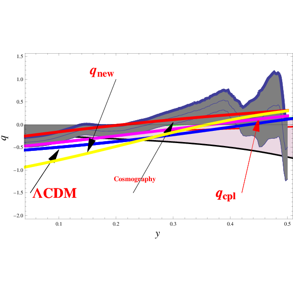
we can reconstruct also . This approach has the advantage to be free from any assumptions about the nature of the dark energy, but it introduces rather large errors in the estimation of , since the numerical derivation is very sensitive to the size and quality of data. In Fig. (6), we compare the obtained by Daly & Djorgovski from their full dataset with the , reconstructed by using Eq. 24 for any considered EOS parametrization, and also the cosmographic . It is interesting to note the cosmographically reconstructed lies completely within the region allowed by the data.
5 Discussion and Conclusions
In this work we have presented constraints on the dark energy EOS obtained by using an updated collection of observational datasets. In particular we are looking for any indications of a deviation from the come to light, reflecting the possibility of a deviation from the CDM cosmological model. To accomplish this task we focus on a direct and full reconstruction of the dark energy EOS through several parametrizations, widely used in literature. We have found indications for a time evolution of the EOS in any considered parametrization, even if the cosmological constant is not ruled out from these observations. To discriminate between different models, we use the so called BIC as selection criterion[Schwarz 1978]: it turns out that the CPL parametrization is favoured by the data. Actually, we evaluated BIC for each model, relative to the CPL model: it turns out that , only for the 3D-parametrization , pointing out a strong evidence against this model. In the case of the oscillating EOS we find out , underlying a certain (weak) positive evidence against such parametrization. It turns out tha for the CPL parametrization , and the the range of confidence at is ; and Moreover, it turns out that if we include in the space of parameters the priors on the values of and obtained from the cosmographic analysis, the constraints on the EOS can be improved competitively with the improvements achieved with future high redshift SNeIa samples : the the range of confidence are, indeed, squeezed at to and . However, since the map connecting the cosmographic and the EOS parameters is highly non linear a strong degeneracy among the parameters is observed, which is hard to manage. Finally, we reconstruct the the deceleration parameter for any considered EOS parametrization, comparing it with the obtained from observational dataset, and with the cosmographic . It is interesting to note that just this lies within the region allowed by the data, thus indicating that a possible strategy to ameliorate the EOS analysis and taking into the account the cosmography results, could consist of setting up a sort of constrained maximum likelihood estimate within the MCMCs, as we intend to perform in an upcoming paper.
Acknowledgments
EP, MDL and PS acknowledge the support of INFN Sez. di Napoli (iniziativa Specifica CQSKY), and also EP and MDL acknowledge the support of INFN Sez. di Napoli (Iniziativa Specifica TEONGRAV). MDL is supported by MIUR (PRIN 2009).
References
- [Amati et al. 2002] Amati L. et al., 2002, A&A, 390, 81
- [Amati 2006] Amati L., 2006, MNRAS, 372, 233
- [Amati et al. 2008] Amati, L., Guidorzi, C., Frontera, F., et al. 2008, MNRAS, 391, 577
- [Amati et al. 2009] Amati, L., Frontera, F.,Guidorzi, C., 2009, A&A, 508, 173
- [Amanullah et al. 2010] Amanullah, R., Lidman, C., Rubin, D., Aldering, G., Astier, P., Barbary, K., Burns, M. S., Conley, A., and collaborators, 2010, ApJ, 716, 71298
- [Schwarz 1978] Schwarz, G. 1978, Ann. Stat. 6, 461
- [Bond et al. 1997] Bond, J.R., Efstathiou, G., Tegmark, M. 1997, MNRAS, 291, L33
- [Antonelli 2009] Antonelli A.L. et al., 2009, A&A, 507, L45
- [Astier et al. 2006] Astier, P., Guy, J., Regnault, N., Pain, R., Aubourg, E. et al. 2006, A&A, 447, 31
- [Bradley 2003] Bradley, S., 2003 ApJ, 583, L67
- [Basilakos & Perivolaropoulos 2008] Basilakos, S., Perivolaropoulos, L. 2008, MNRAS, 391, 411
- [Bloom et al. 2003] Bloom, J.S., Frail, D.A., Kulkarini,S. R., 2003, ApJ, 594, 674
- [Butler et al. 2007] Butler N.R. et al., 2007, ApJ, 671, 656
- [Capozziello and De Laurentis2011] Capozziello S., De Laurentis M., 2011, Physics Reports, 509, 167.
- [Capozziello, Lazkoz, and Salzano 2011] Capozziello, S., Lazkoz, R., Salzano, V., 2011, Phys. Rev. D, 84, 124061
- [Efstathiou & Bond 1999] Efstathiou, G., Bond, J.R. 1999, MNRAS, 304, 75
- [Eisenstein et al. 2005] Eisenstein, D.J., Zehavi, I., Hogg, D.W., Scoccimarro, R., Blanton, M.R. et al. 2005, ApJ, 633, 560
- [Chevallier and Polarski 2001] Chevallier,M., Polarski, D., 2001, Int. J. Mod. Phys. D10 213-224
- [Clarkson and Zunckel 2010] Clarkson, C., and Zunckel, C., 2010, Phys. Rev. Lett. bf 104, 211301
- [Lazkoz, Salzano and Sendra 2010] Lazkoz, R., Salzano, V., Sendra,I., Revisiting a model-independent dark energy reconstruction method, [arXiv:1202.4689 [astro-ph.CO]].
- [Linder 2003] E. V. Linder, 2003, Phys. Rev. Lett. 90 091301.
- [Colgate 1979] Colgate, S. A., 1979, ApJ, 232, 404
- [Collazzi et al. 2005] Collazzi,A.C., Schaefer, B., Goldstein, A., Preece, R., D., 2011, arXiv:1112.4347
- [D’Agostini 2005] D’Agostini, G., 2005, arXiv : physics/051182
- [Dai et al. 2004] Dai, Z.G., Liang, E.W., Xu, D. 2004, ApJ, 612, L101
- [Daly and Djorgovski 2003] Daly, R.A., Djorgovski, S. G. ,Astrophys. J. 597 (2003) 9.
- [Daly and Djorgovski 2004] Daly, R.A., Djorgovski, S. G. , Astrophys. J. 612 (2004) 652.
- [Daly and Djorgovski 2008] Daly, R.A., Djorgovski, S. G. , Astrophys. J. 677 (2008) 1.
- [Demianski et al.2003] Demianski, M., de Ritis, R., Marino, A. A., Piedipalumbo, E., 2003, A&A, 411,33
- [Demianski et al. 2005] Demianski, M., Piedipalumbo, E., Rubano, C., Tortora, C., 2005, A&A, 431, 27
- [Demianski, Piedipalumbo and Rubano 2011] Demianski, M., Piedipalumbo, E., Rubano, C., 2011, MNRAS, 411, 1213
- [Demianski & Piedipalumbo 2011] Demianski, M., Piedipalumbo, 2011, MNRAS, 415, 3580
- [Demianski et al. 2012] Demianski, M., Piedipalumbo, E., Rubano, C. and Scudellaro, P. , 2012, MNRAS, 426: 13961415.
- [Diaferio et al. 2011] Diaferio A., Ostorero L., Cardone V.F., 2011, arXiv:1103.5501
- [di Serafino et al. 2010] di Serafino,D., Gmez, S., Milano, L., Riccio, F., Toraldo, G., 2010, J. Global Optimization, 48(1), 41.
- [di Serafino & Riccio 2010] di Serafino, D. , Riccio, F., 2010, PDP, 231-237.
- [Firmani at al. 1998] Eisenstein,D.J., Hu, W., 1998, ApJ, 496, 605
- [Firmani at al. 2005] Firmani C., Ghisellini, G., Ghirlanda, Avila - Reese, G., 2005, MNRAS,360, L1
- [Gao et al. 2010] Gao, H., Liang, N., Zhu, Z.-H., 2010, eprint arXiv:1003.5755
- [Ghirlanda at al. 2005] Ghirlanda G., Ghisellini G. and Firmani C., 2005, MNRAS, 361, L10.
- [Ghirlanda et al.2008] Ghirlanda, G., Nava, L., Ghisellini, G., Firmani, C., Cabrera, J. I. 2008, MNRAS, 387, 319
- [Ghisellini et al. 2009] Ghisellini G., Nardini, M., Ghirlanda, G., Celotti, A., 2009, MNRAS, 393,16
- [Greiner et al. 2009] Greiner, J., Kruehler, T., Fynbo, J.P.U., Rossi, A., Schwarz, R. et al., 2009, ApJ, 693, 1610
- [Lamb et al. 2005] Lamb, D. Q., Donaghy, T. Q., Graziani, C., 2005, ApJ, 620, 355
- [Kantowski1998] Kantowski R., 1998, ApJ, 507, 483
- [Kantowski, Kao & Thomas 2000] Kantowski R., Kao J.K., Thomas, R.C., 2000, ApJ, 545, 549
- [Kantowski & Thomas 2001] Kantowski R., and Thomas, R.C., 2001, ApJ, 561, 491
- [Lazkoz, Salzano and Sendra 2010] Lazkoz, R., Salzano, V., Sendra, I., 2010, Phys.Lett.B, 694, 198-208
- [Lazkoz, Salzano and Sendra 2012] Lazkoz, R., Salzano, V., Sendra, I., 2012,Eur. Phys. J. C 72, 2130
- [Li et al. 2008] Li, H., Su, M., Fan, Z., Dai, Z., Zhang, X., 2008, Phys. Lett. B, 658, 95
- [Liang et al. 2008] Liang, N., Xiao, W. K., Liu, Y., Zhang, S. N., 2008, ApJ, in press, arXiv:0802.4262
- [Kowalski et al. 2008] Kowalski, M., Rubin, D., Aldering, G., Agostinho, R.J, Amadon, A. et al., 2008, arXiv :0804.4142
- [Ma & Zhang 2011] Ma, J-Z., Zhang, Z., 2011, Physics Letters B, 699, 233-238
- [Meszaros 2006] Meszaros, P., 2006, Rep. Prog. Phys., 69, 2259
- [Nakar & Piran 2005] Nakar, E., Piran, T., 2005, MNRAS, 360, L73
- [Nesseris and Bellido 2012] Nesseris, S and Garcia - Bellido J.,2012, JCAP, 1211, 033
- [Riess et al. 2007] Riess, A.G., Strolger, L.G., Casertano, S., Ferguson, H.C., Mobasher, B. et al., 2007, ApJ, 659, 98
- [Riess et al. 2009] Riess, A.G., Macri, L., Li, W., Lampeitl, H., Casertano, S. et al. 2009, ApJ 699, 539
- [Rubano & Scudellaro 2002] Rubano, C., Scudellaro, P., 2002, Gen. Rel. Grav., 34, 307
- [Rubano & Scudellaro 2002] Rubano, C., Scudellaro, P., 2002, Gen. Rel. Grav., 34, 1931
- [Pavlov et al. 2002] Pavlov, M., Rubano, C., Sahzin, M.V., Scudellaro, P., 2002, Astrophys.J. 566, 619-622
- [Percival al. 2010] Percival, W.J., Reid, B.A., Eisenstein, D.J., Bahcall, N.A., Budavari, T., et al., 2010, MNRAS, 401, 2148
- [Perlmutter et al. 1999] Perlmutter, S., Aldering, G., Goldhaber, G., Knop, R. A., Nugent, P., et al. 1999, ApJ, 517, 565
- [Planck Collaboartion 2013] Planck Collaboartion, Planck 2013 results. XVI. Cosmological parameters, arXiv:1303.5076 [astro-ph.CO].
- [Rubano et al. 2004] Rubano C., Scudellaro P., Piedipalumbo E., Capozziello S., Capone M., 2004, Phys.Rev.D, 69, 103510
- [Sahni et al. 2003] Sahni, V., Saini, T.D., Starobinsky, A.A., Alam, U., 2003, JETP Lett., 77, 201;
- [Sakamoto et al. 2008] Sakamoto T. et al., 2008, ApJ Supp., 175, 179
- [ Sahni and Starobinsky2006] Sahni, V., and Starobinsky, A., 2006,Int.J. Mod. Phys. D, 15, 2105
- [ Said et al.2013] Sahni N., Baccigalupi C., Martinelli M., Melchiorri A., Silvestri A., 2013, New Constraints On The Dark Energy Equation of State, arXiv:1303.4353 [astro-ph.CO]
- [Schaefer 2003] Schaefer, B.E., 2003, ApJ, 583, L67
- [Schaefer 2007] Schaefer, B.E., 2007, ApJ, 660, 16
- [ Shafieloo, Sahni, and Starobinsky 2009] Shafieloo, A., Sahni, V., Starobinsky, A.A., 2009, Phys. Rev. D 80, 101301
- [Riess et al. 1998] Riess, A.G., Filippenko, A. V., Challis, P., Clocchiatti, A., Diercks, A., et al., 1998, ApJ, 116,1009
- [Salzano et al. 2013] Salzano V., Rodney S. A., Sendra I., Lazkoz R., Riess A.G., Postmann M., Broadhurst T., Coe D., 2013, Improving Dark energy Constraints with High Redshift Type Ia Supernovae from CANDLES and CLASH, arXiv:1307.0820 [astro-ph.CO].
- [Suzuki et al. 2012] Suzuki et al. (The Supernova Cosmology Project), 2012, ApJ, 746, 85
- [Spergel et al. 2007] Spergel, D.N., et al., 2007, ApJS, 170, 377
- [Tsutsui et al. 2009] Tsutsui, R., Nakamura, T., Yonetoku, D., Murakami, T., Tanabe, S., et al., 2009, MNRAS, 394, L31-L35
- [Visser 2004] Visser, M, 2004, Class. Quant. Grav., 21, 2603
- [Vitagliano et al. 2010] Vitagliano, V., Xia, J.Q., Liberati, S., Viel, M., 2010, JCAP, 3, 005
- [Wang 2008] Wang, Y., 2008, Phys. Rev. D, 78, 123532
- [Wang, Deng and Qiu 2008] Wang, J., Deng, J.S., and Qiu, Y.J., 2008, Chin. J. Astron. Astrophys., 8, 255
- [Wei 2010] Wei, H., 2010, JCAP, 8, 20
- [Wood - Vasey et al. 2007] Wood - Vasey, W.M., Miknaitis, G., Stubbs, C.W., Jha, S., Riess, A.G., et al., 2007, ApJ, 666, 694
- [Komatsu et al. 2010] Komatsu, E., Smith, K.M., Dunkley, J., Bennett, C.L., Gold, B. et al. 2010, preprint arXiv :1001.4538