跳到论文正文
W Papers独立论文阅读器 arXiv:1311.0830 论文正文 计算阅读时间 · 0%
引用这篇论文根据当前论文元数据生成,正式投稿前建议核对。


License: arXiv.org perpetual non-exclusive license
arXiv:1311.0830v2 [cs.IT] 06 Nov 2013

The Squared-Error of Generalized LASSO:
A Precise Analysis

Samet Oymak, Christos Thrampoulidis and Babak Hassibi ††thanks: This work was supported in part by the National Science Foundation under grants CCF-0729203, CNS-0932428 and CIF-1018927, by the Office of Naval Research under the MURI grant N00014-08-1-0747, and by a grant from Qualcomm Inc. Affiliation: Department of Electrical Engineering Affiliation: Caltech, Pasadena – 91125 Affiliation: soymak@caltech.edu, cthrampo@caltech.edu, hassibi@caltech.edu
Abstract

We consider the problem of estimating an unknown signal 𝐱0\mathbf{x}_{0} from noisy linear observations 𝐲=𝐀𝐱0+𝐳∈ℝm\mathbf{y}=\mathbf{A}\mathbf{x}_{0}+\mathbf{z}\in\mathbb{R}^{m}. In many practical instances of this problem, 𝐱0\mathbf{x}_{0} has a certain structure that can be captured by a structure inducing function f⁡(⋅)f(\cdot). For example, ℓ1\ell_{1} norm can be used to encourage a sparse solution. To estimate 𝐱0\mathbf{x}_{0} with the aid of a convex f⁡(⋅)f(\cdot), we consider three variations of the widely used L​A​S​S​OLASSO estimator and provide sharp characterizations of their performances. Our study falls under a generic framework, where the entries of the measurement matrix 𝐀\mathbf{A} and the noise vector 𝐳\mathbf{z} have zero-mean normal distributions with variances 11 and σ2\sigma^{2}, respectively. For the LASSO estimator 𝐱∗\mathbf{x}^{*}, we ask: “What is the precise estimation error as a function of the noise level σ\sigma, the number of observations mm and the structure of the signal?". In particular, we attempt to calculate the Normalized Square Error (NSE) defined as ‖𝐱∗−𝐱0‖22σ2\frac{\|\mathbf{x}^{*}-\mathbf{x}_{0}\|_{2}^{2}}{\sigma^{2}}. We show that, the structure of the signal 𝐱0\mathbf{x}_{0} and choice of the function f⁡(⋅)f(\cdot) enter the error formulae through the summary parameters 𝐃f​(𝐱0,ℝ+){\mathbf{D}}_{f}(\mathbf{x}_{0},{\mathbb{R}}^{+}) and 𝐃f​(𝐱0,λ){\mathbf{D}}_{f}(\mathbf{x}_{0},{\lambda}), which are defined as the “Gaussian squared-distances” to the subdifferential cone and to the λ\lambda-scaled subdifferential of ff at 𝐱0\mathbf{x}_{0}, respectively. The first estimator assumes a-priori knowledge of f⁡(𝐱0)f(\mathbf{x}_{0}) and is given by argmin𝐱{∥𝐲−𝐀𝐱∥2subject tof(𝐱)≤f(𝐱0)}\arg\min_{\mathbf{x}}\left\{{\|\mathbf{y}-\mathbf{A}\mathbf{x}\|_{2}}~\text{subject to}~f(\mathbf{x})\leq f(\mathbf{x}_{0})\right\}. We prove that its worst case NSE is achieved when σ→0\sigma\rightarrow 0 and concentrates around 𝐃f​(𝐱0,ℝ+)m−𝐃f​(𝐱0,ℝ+)\frac{{\mathbf{D}}_{f}(\mathbf{x}_{0},{\mathbb{R}}^{+})}{m-{\mathbf{D}}_{f}(\mathbf{x}_{0},{\mathbb{R}}^{+})}. Secondly, we consider arg⁡min𝐱​{‖𝐲−𝐀𝐱‖2+λ​f​(𝐱)}\arg\min_{\mathbf{x}}\left\{\|\mathbf{y}-\mathbf{A}\mathbf{x}\|_{2}+{\lambda}f(\mathbf{x})\right\}, for some penalty parameter λ≥0{\lambda}\geq 0. This time, the NSE formula depends on the choice of λ\lambda and is given by 𝐃f​(𝐱0,λ)m−𝐃f​(𝐱0,λ)\frac{{\mathbf{D}}_{f}(\mathbf{x}_{0},{\lambda})}{m-{\mathbf{D}}_{f}(\mathbf{x}_{0},{\lambda})} over a range of λ{\lambda}. The last estimator is arg⁡min𝐱​{12​‖𝐲−𝐀𝐱‖22+σ​τ​f​(𝐱)}\arg\min_{\mathbf{x}}\left\{\frac{1}{2}\|\mathbf{y}-\mathbf{A}\mathbf{x}\|_{2}^{2}+\sigma\tau f(\mathbf{x})\right\}. We establish a mapping between this and the second estimator and propose a formula for its NSE. As useful side results, we find explicit formulae for the optimal estimation performance and the optimal penalty parameters λbest\lambda_{\text{best}} and τb​e​s​t\tau_{best}. Finally, for a number of important structured signal classes, we translate our abstract formulae to closed-form upper bounds on the NSE.

Keywords: convex optimization, generalized LASSO, structured sparsity, Gaussian processes, statistical estimation, duality, model fitting, linear inverse, first order approximation, noisy compressed sensing, random noise

1. Introduction

1.1.   The Generalized LASSO Problem

Recovering a structured signal 𝐱0∈ℝn\mathbf{x}_{0}\in\mathbb{R}^{n} from a vector of limited and noisy linear observations 𝐲=𝐀𝐱0+𝐳∈ℝm\mathbf{y}=\mathbf{A}\mathbf{x}_{0}+\mathbf{z}\in\mathbb{R}^{m}, is a problem of fundamental importance encountered in several disciplines including machine learning, signal processing, network inference and many more [1, 2, 3, 4]. A typical approach for estimating the structured signal 𝐱0\mathbf{x}_{0} from the measurement vector 𝐲\mathbf{y}, is picking some proper structure inducing function f⁡(⋅)f(\cdot) and solving the following problem

𝐱L​A​S​S​O∗=argmin𝐱{12​‖𝐲−𝐀𝐱‖22+λ​f​(𝐱)},\mathbf{x}^{*}_{LASSO}=\operatorname*{argmin}_{\mathbf{x}}\left\{~\frac{1}{2}\|\mathbf{y}-\mathbf{A}\mathbf{x}\|_{2}^{2}+{\lambda}f(\mathbf{x})~\right\}, (1.1)

for some nonnegative penalty parameter λ\lambda.

In case 𝐱0\mathbf{x}_{0} is a sparse vector, the associated structure inducing function is the ℓ1\ell_{1} norm, i.e. f⁡(𝐱)=‖𝐱‖1f(\mathbf{x})=\|\mathbf{x}\|_{1}. The resulting ℓ1\ell_{1}-penalized quadratic program in (1.1) is known as the LASSO in the statistics literature. LASSO was originally introduced in [5] and has since then been subject of great interest as a natural and powerful approach to do noise robust compressed sensing (CS), [5, 6, 7, 14, 15, 8, 13, 9, 11, 10, 12]. There are also closely related algorithms such as SOCP variations and the Dantzig selector [18, 19]. Of course, applications of (1.1) are not limited to sparse recovery; they extend to various problems including the recovery of block sparse signals [21, 20], the matrix completion problem [23, 22] and the total variation minimization [24]. In each application, f⁡(⋅)f(\cdot) is chosen in accordance to the structure of 𝐱0\mathbf{x}_{0}. See [25] for additional examples and a principled approach to constructing such penalty functions. In this work, we consider arbitrary convex penalty functions f⁡(⋅)f(\cdot) and we commonly refer to this generic formulation in (1.1) as the “Generalized LASSO" or simply “LASSO" problem.

1.2.   Motivation

The LASSO problem can be viewed as a “merger" of two closely related problems, which have both recently attracted a lot of attention by the research community; the problems of noiseless CS and that of proximal denoising.

1.2.1 Noiseless compressed sensing

In the noiseless CS problem one wishes to recover 𝐱0\mathbf{x}_{0} from the random linear measurements 𝐲=𝐀𝐱0\mathbf{y}=\mathbf{A}\mathbf{x}_{0}. A common approach is solving the following convex optimization problem

min𝐱⁡f⁡(𝐱)​subject to​𝐲=𝐀𝐱.\min_{\mathbf{x}}f(\mathbf{x})~~~\text{subject to}~~~\mathbf{y}=\mathbf{A}\mathbf{x}. (1.2)

A critical performance criteria for the problem (1.2) concerns the minimum number of measurements needed to guarantee successful recovery of 𝐱0\mathbf{x}_{0} [26, 30, 28, 27, 29, 25, 31]. Here, success means that 𝐱0\mathbf{x}_{0} is the unique minimizer of (1.2), with high probability, over the realizations of the random matrix 𝐀\mathbf{A}.

1.2.2 Proximal denoising

The proximal denoising problem tries to estimate 𝐱0\mathbf{x}_{0} from noisy but uncompressed observations 𝐲=𝐱0+𝐳\mathbf{y}=\mathbf{x}_{0}+\mathbf{z}, 𝐳∼𝒩⁡(0,σ2​𝐈n)\mathbf{z}\sim\mathcal{N}(0,\sigma^{2}\mathbf{I}_{n}), where we write 𝐈k\mathbf{I}_{k} for the identity matrix of size k×kk\times k, k∈ℤ+k\in\mathbb{Z}^{+}. In particular, it solves,

min𝐱⁡{12​‖𝐲−𝐱‖22+λ​σ​f​(𝐱)}.\min_{\mathbf{x}}\left\{\frac{1}{2}\|\mathbf{y}-\mathbf{x}\|_{2}^{2}+{\lambda}\sigma f(\mathbf{x})\right\}. (1.3)

A closely related approach to estimate 𝐱0\mathbf{x}_{0}, which requires prior knowledge f⁡(𝐱0)f(\mathbf{x}_{0}) about the signal of interest 𝐱0\mathbf{x}_{0}, is solving the constrained denoising problem:

min𝐱⁡‖𝐲−𝐱‖22​subject to​f​(𝐱)≤f⁡(𝐱0).\min_{\mathbf{x}}\|\mathbf{y}-\mathbf{x}\|_{2}^{2}~~~\text{subject to}~~~f(\mathbf{x})\leq f(\mathbf{x}_{0}). (1.4)

The natural question to be posed in both cases is how well can one estimate 𝐱0\mathbf{x}_{0} via (1.3) (or (1.4)) [40, 44, 43, 41, 42]? The minimizer 𝐱∗\mathbf{x}^{*} of (1.3) (or (1.4)) is a function of the noise vector 𝐳\mathbf{z} and the common measure of performance, is the normalized mean-squared-error which is defined as 𝔼​‖𝐱∗−𝐱0‖22σ2.\frac{{\mathbb{E}}\|\mathbf{x}^{*}-\mathbf{x}_{0}\|_{2}^{2}}{\sigma^{2}}.

1.2.3 The “merger" LASSO

The Generalized LASSO problem is naturally merging the problems of noiseless CS and proximal denoising. The compressed nature of measurements, poses the question of finding the minimum number of measurements required to recover 𝐱0\mathbf{x}_{0} robustly, that is with error proportional to the noise level. When recovery is robust, it is of importance to be able to explicitly characterize how good the estimate is. In this direction, when 𝐳∼𝒩⁡(0,σ2​𝐈m)\mathbf{z}\sim\mathcal{N}(0,\sigma^{2}\mathbf{I}_{m}), a common measure of performance for the LASSO estimate 𝐱L​A​S​S​O∗\mathbf{x}^{*}_{LASSO} is defined to be the normalized squared error (NSE) :

N​S​E=1σ2​‖𝐱L​A​S​S​O∗−𝐱0‖22.NSE=\frac{1}{\sigma^{2}}\|\mathbf{x}^{*}_{LASSO}-\mathbf{x}_{0}\|^{2}_{2}.

This is exactly the main topic of this work: proving precise bounds for the NSE of the Generalized LASSO problem.

In the specific case of ℓ1\ell_{1}-penalization in (1.1), researchers have considered other performance criteria additional to the NSE [10, 12, 11]. As an example, we mention the support recovery criteria [10], which measures how well (1.1) recovers the subset of nonzero indices of 𝐱0\mathbf{x}_{0}. However, under our general setup, where we allow arbitrary structure to the signal 𝐱0\mathbf{x}_{0}, the NSE serves as the most natural measure of performance and is, thus, the sole focus in this work. In the relevant literature, researchers have dealt with the analysis of the NSE of (1.1) under several settings (see Section 1.4). Yet, we still lack a general theory that would yield precise bounds for the squared-error of (1.1) for arbitrary convex regularizer f⁡(⋅)f(\cdot). This paper aims to close this gap. Our answer involves inherent quantities regarding the geometry of the problem which, in fact, have recently appeared in the related literature, [25, 31, 32, 15, 14, 41].

1.3.   Three Versions of the LASSO Problem

Throughout the analysis, we assume 𝐀∈ℝm×n\mathbf{A}\in\mathbb{R}^{m\times n} has independent standard normal entries and 𝐳∼𝒩⁡(0,σ2​𝐈m)\mathbf{z}\sim\mathcal{N}(0,\sigma^{2}\mathbf{I}_{m}). Our approach tackles various forms of the LASSO all at once, and relates them to each other. In particular, we consider the following three versions:

  • ⋆\star

    C-LASSO: Assumes a-priori knowledge of f⁡(𝐱0)f(\mathbf{x}_{0}) and solves,

    𝐱c∗​(𝐀,𝐳)=arg​min𝐱​‖𝐲−𝐀𝐱‖2​subject to​f​(𝐱)≤f⁡(𝐱0).\mathbf{x}_{c}^{*}(\mathbf{A},\mathbf{z})=\text{arg}\min_{\mathbf{x}}\|\mathbf{y}-\mathbf{A}\mathbf{x}\|_{2}~~~\text{subject to}~~~f(\mathbf{x})\leq f(\mathbf{x}_{0}).\vskip-1.0pt (1.5)
  • ⋆\star

    ℓ2\ell_{2}-LASSO: Uses ℓ2\ell_{2}-penalization rather than ℓ22\ell_{2}^{2} and solves,

    𝐱ℓ2∗​(λ,𝐀,𝐳)=arg​min𝐱​{‖𝐲−𝐀𝐱‖2+λ​f​(𝐱)}.\mathbf{x}_{\ell_{2}}^{*}({\lambda},\mathbf{A},\mathbf{z})=\text{arg}\min_{\mathbf{x}}\left\{~\|\mathbf{y}-\mathbf{A}\mathbf{x}\|_{2}+{\lambda}f(\mathbf{x})~\right\}.\vskip-8.0pt (1.6)
  • ⋆\star

    ℓ22\ell_{2}^{2}-LASSO: the original form given in (1.1) :

    𝐱ℓ22∗​(τ,𝐀,𝐳)=arg​min𝐱​{12​‖𝐲−𝐀𝐱‖22+σ​τ​f​(𝐱)}.\displaystyle\mathbf{x}_{\ell_{2}^{2}}^{*}(\tau,\mathbf{A},\mathbf{z})=\text{arg}\min_{\mathbf{x}}\left\{~\frac{1}{2}\|\mathbf{y}-\mathbf{A}\mathbf{x}\|_{2}^{2}+\sigma\tau f(\mathbf{x})~\right\}. (1.7)

C-LASSO in (1.5) stands for “Constrained LASSO". This version of the LASSO problem assumes some a-priori knowledge about 𝐱0\mathbf{x}_{0}, which makes the analysis of the problem arguably simpler than that of the other two versions, in which the role of the penalty parameter (which is meant to compensate for the lack of a-priori knowledge) has to be taken into consideration. To distinguish between the ℓ2\ell_{2}-LASSO and the ℓ22\ell_{2}^{2}-LASSO, we use λ{\lambda} to denote the penalty parameter of the former and τ\tau for the penalty parameter of the latter. Part of our contribution is establishing useful connections between these three versions of the LASSO problem. We will often drop the arguments λ,τ,𝐀,𝐳{\lambda},\tau,\mathbf{A},\mathbf{z} from the LASSO estimates defined in (1.5)–(1.7), when clear from context.

1.4.   Relevant Literature

Precise characterization of the NSE of the LASSO is closely related to the precise performance analysis of noiseless CS and proximal denoising. To keep the discussion short, we defer most of the comments on the connections of our results to these problems to the main body of the paper. Table 1 provides a summary of the relevant literature and highlights the area of our contribution.

Convex functions ℓ1\ell_{1}-minimization
Noiseless CS Chandrasekaran et al. [25] Amelunxen et al. [31] Donoho and Tanner, [28] Stojnic, [26]
Proximal
denoising
Donoho et al. [44] Oymak and Hassibi[41] Donoho [40]
LASSO Present paper Bayati and Montanari, [14], [15] Stojnic, [37]
Table 1: Relevant Literature.

The works closest in spirit to our results include [14, 15, 37, 16], which focus on the exact analysis of the LASSO problem, while restricting the attention on sparse recovery where f⁡(𝐱)=‖𝐱‖1f(\mathbf{x})=\|\mathbf{x}\|_{1} . In [14, 15], Bayati and Montanari are able to show that the mean-squared-error of the LASSO problem is equivalent to the one achieved by a properly defined “Approximate Message Passing” (AMP) algorithm. Following this connection and after evaluating the error of the AMP algorithm, they obtain an explicit expression for the mean squared error of the LASSO algorithm in an asymptotic setting. In [16], Maleki et al. proposes Complex AMP, and characterizes the performance of LASSO for sparse signals with complex entries. In [37], Stojnic’s approach relies on results on Gaussian processes [72, 73] to derive sharp bounds for the worst case NSE of the ℓ1\ell_{1}-constrained LASSO problem in (1.5). Our approach in this work builds on the framework proposed by Stojnic, but extends the results in multiple directions as noted in the next section.

1.5.   Contributions

This section summarizes our main contributions. In short, this work:

  • •

    generalizes the results of [37] on the constrained LASSO for arbitrary convex functions; proves that the worst case NSE is achieved when the noise level σ→0\sigma\rightarrow 0, and derives sharp bounds for it.

  • •

    extends the analysis to the NSE of the more challenging ℓ2\ell_{2}-LASSO; provides bounds as a function of the penalty parameter λ{\lambda}, which are sharp when σ→0\sigma\rightarrow 0.

  • •

    identifies a connection between the ℓ2\ell_{2}-LASSO to the ℓ22\ell_{2}^{2}-LASSO; proposes a formula for precisely calculating the NSE of the latter when σ→0\sigma\rightarrow 0.

  • •

    provides simple recipes for the optimal tuning of the penalty parameters λ{\lambda} and τ\tau in the ℓ2\ell_{2} and ℓ22\ell_{2}^{2}-LASSO problems.

  • •

    analyzes the regime in which stable estimation of 𝐱0\mathbf{x}_{0} fails.

1.6.   Motivating Examples

Before going into specific examples, it is instructive to consider the scenario where f⁡(⋅)=0f(\cdot)=0. This reduces the problem to a regular least-squares estimation problem, the analysis of which is easy to perform. When m<nm<n, the system is underdetermined, and one cannot expect 𝐱∗\mathbf{x}^{*} to be a good estimate. When m≥nm\geq n, the estimate can be given by 𝐱∗=(𝐀T​𝐀)−1​𝐀T​𝐲\mathbf{x}^{*}=(\mathbf{A}^{T}\mathbf{A})^{-1}\mathbf{A}^{T}\mathbf{y}. In this case, the normalized mean-squared-error takes the form,

𝔼​‖𝐱∗−𝐱0‖2σ2=𝔼⁡[𝐳T​𝐀​(𝐀T​𝐀)−2​𝐀T​𝐳]σ2=𝔼⁡[trace​(𝐀​(𝐀T​𝐀)−2​𝐀T)]=𝔼⁡[trace​((𝐀T​𝐀)−1)].\frac{{\mathbb{E}}\|\mathbf{x}^{*}-\mathbf{x}_{0}\|^{2}}{\sigma^{2}}=\frac{{\mathbb{E}}[\mathbf{z}^{T}\mathbf{A}(\mathbf{A}^{T}\mathbf{A})^{-2}\mathbf{A}^{T}\mathbf{z}]}{\sigma^{2}}={\mathbb{E}}[{\text{trace}(\mathbf{A}(\mathbf{A}^{T}\mathbf{A})^{-2}\mathbf{A}^{T})}]={\mathbb{E}}[{\text{trace}((\mathbf{A}^{T}\mathbf{A})^{-1})}].

𝐀T​𝐀\mathbf{A}^{T}\mathbf{A} is a Wishart matrix and its inverse is well studied. In particular, when m≥n+2m\geq n+2, we have 𝔼⁡[(𝐀T​𝐀)−1]=𝐈nm−n−1{\mathbb{E}}[(\mathbf{A}^{T}\mathbf{A})^{-1}]=\frac{\mathbf{I}_{n}}{m-n-1} (see [70]). Hence,

𝔼​‖𝐱∗−𝐱0‖2σ2=nm−n−1.\frac{{\mathbb{E}}\|\mathbf{x}^{*}-\mathbf{x}_{0}\|^{2}}{\sigma^{2}}=\frac{n}{m-n-1}. (1.8)

How does this result change when a nontrivial convex function f⁡(⋅)f(\cdot) is introduced?

Our message is simple: when f⁡(⋅)f(\cdot) is an arbitrary convex function, the LASSO error formula is obtained by simply replacing the ambient dimension nn in (1.8) with a summary parameter 𝐃f​(𝐱0,ℝ+){\mathbf{D}}_{f}(\mathbf{x}_{0},{\mathbb{R}}^{+}) or 𝐃f​(𝐱0,λ){\mathbf{D}}_{f}(\mathbf{x}_{0},{\lambda}) . These parameters are defined as the expected squared-distance of a standard normal vector in ℝn\mathbb{R}^{n} to the conic hull of the subdifferential cone​(∂f​(𝐱0))\text{cone}(\partial f(\mathbf{x}_{0})) and to the scaled subdifferential λ​∂f⁡(𝐱0){\lambda}\partial f(\mathbf{x}_{0}), respectively. They summarize the effect of the structure of the signal 𝐱0\mathbf{x}_{0} and choice of the function f⁡(⋅)f(\cdot) on the estimation error.

To get a flavor of the (simple) nature of our results, we briefly describe how they apply in three commonly encountered settings, namely the “sparse signal", “low-rank matrix" and “block-sparse signal" estimation problems. For simplicity of exposition, let us focus on the C-LASSO estimator in (1.5). A more elaborate discussion, including estimation via ℓ2\ell_{2}-LASSO and ℓ22\ell_{2}^{2}-LASSO, can be found in Section 4.4. The following statements are true with high probability in 𝐀,𝐯\mathbf{A},\mathbf{v} and hold under mild assumptions.

​1~~\emph{1}. Sparse signal estimation: Assume 𝐱0∈ℝn\mathbf{x}_{0}\in\mathbb{R}^{n} has kk nonzero entries. In order to estimate 𝐱0\mathbf{x}_{0}, use the Constrained-LASSO and pick ℓ1\ell_{1}-norm for f⁡(⋅)f(\cdot). Let m>2​k​(log⁡nk+1)m>2k(\log\frac{n}{k}+1). Then,

‖𝐱c∗−𝐱0‖22σ2≲2​k​(log⁡nk+1)m−2​k​(log⁡nk+1).\frac{\|\mathbf{x}^{*}_{c}-\mathbf{x}_{0}\|_{2}^{2}}{\sigma^{2}}\lesssim\frac{2k(\log{\frac{n}{k}+1)}}{m-2k(\log\frac{n}{k}+1)}. (1.9)

​2~~\emph{2}. Low-rank matrix estimation: Assume 𝐗0∈ℝd×d\mathbf{X}_{0}\in\mathbb{R}^{d\times d} is a rank rr matrix, n=d×dn=d\times d. This time, 𝐱0∈ℝn\mathbf{x}_{0}\in\mathbb{R}^{n} corresponds to vectorization of 𝐗0\mathbf{X}_{0} and f⁡(⋅)f(\cdot) is chosen as the nuclear norm ∥⋅∥⋆\|\cdot\|_{\star} (sum of the singular values of a matrix) [51, 50]. Hence, we observe 𝐲=𝐀⋅vec​(𝐗0)+𝐳\mathbf{y}=\mathbf{A}\cdot\text{vec}(\mathbf{X}_{0})+\mathbf{z} and solve,

min𝐗∈ℝd×d⁡‖𝐲−𝐀⋅vec​(𝐗)‖2​subject to​‖𝐗‖⋆≤‖𝐗0‖⋆\min_{\mathbf{X}\in\mathbb{R}^{d\times d}}\|\mathbf{y}-\mathbf{A}\cdot\text{vec}(\mathbf{X})\|_{2}~~~\text{subject to}~~~\|\mathbf{X}\|_{\star}\leq\|\mathbf{X}_{0}\|_{\star}

Let m>6​d​rm>6dr. Denote the LASSO estimate by 𝐗c∗\mathbf{X}_{c}^{*} and use ∥⋅∥F\|\cdot\|_{F} for the Frobenius norm of a matrix. Then,

‖𝐗c∗−𝐗0‖F2σ2≲6​d​rm−6​d​r.\frac{\|\mathbf{X}_{c}^{*}-\mathbf{X}_{0}\|^{2}_{F}}{\sigma^{2}}\lesssim\frac{6dr}{m-6dr}. (1.10)

​3~~\emph{3}. Block sparse estimation: Let n=t×bn=t\times b and assume the entries of 𝐱0∈ℝn\mathbf{x}_{0}\in\mathbb{R}^{n} can be grouped into tt known blocks of size bb so that only kk of these tt blocks are nonzero. To induce the structure, the standard approach is to use the ℓ1,2\ell_{1,2} norm which sums up the ℓ2\ell_{2} norms of the blocks, [46, 47, 48, 49]. In particular, denoting the subvector corresponding to ii’th block of a vector 𝐱\mathbf{x} by 𝐱i\mathbf{x}_{i}, the ℓ1,2\ell_{1,2} norm is equal to ‖𝐱‖1,2=∑i=1t‖𝐱i‖2\|\mathbf{x}\|_{1,2}=\sum_{i=1}^{t}\|\mathbf{x}_{i}\|_{2}. Assume m>4​k​(log⁡tk+b)m>4k(\log\frac{t}{k}+b) . Then,

‖𝐱c∗−𝐱0‖22σ2≲4​k​(log⁡tk+b)m−4​k​(log⁡tk+b).\frac{\|\mathbf{x}_{c}^{*}-\mathbf{x}_{0}\|^{2}_{2}}{\sigma^{2}}\lesssim\frac{4k(\log\frac{t}{k}+b)}{m-4k(\log\frac{t}{k}+b)}. (1.11)

Note how (1.9)-(1.11) are similar in nature to (1.8).

2. Our Approach

In this section we introduce the main ideas that underlie our approach. This will also allow us to introduce important concepts from convex geometry required for the statements of our main results in Section 3. The details of most of the technical discussion in this introductory section are deferred to later sections. To keep the discussion concise, we focus our attention on the ℓ2\ell_{2}-LASSO. Throughout, we use boldface lowercase letters to denote vectors and boldface capital letters to denote matrices. Also, to simplify the notation the ℓ2\ell_{2}-norm will be denoted as ∥⋅∥\|\cdot\| from now on.

2.1.   First-Order Approximation

Recall the ℓ2\ell_{2}-LASSO problem introduced in (1.6):

𝐱ℓ2∗=arg​min𝐱​{‖𝐲−𝐀𝐱‖+λ​f​(𝐱)}.\mathbf{x}^{*}_{\ell_{2}}=\text{arg}\min_{\mathbf{x}}\left\{~\|\mathbf{y}-\mathbf{A}\mathbf{x}\|+{\lambda}f(\mathbf{x})~\right\}.\vskip-8.0pt (2.1)

A key idea behind our approach is using the linearization of the convex structure inducing function f⁡(⋅)f(\cdot) around the vector of interest 𝐱0\mathbf{x}_{0} [86, 77]:

f^​(𝐱)=f⁡(𝐱0)+sup𝐬∈λ​∂f⁡(𝐱0)𝐬T​(𝐱−𝐱0).{\hat{f}}(\mathbf{x})=f(\mathbf{x}_{0})+\sup_{\mathbf{s}\in{\lambda}\partial f(\mathbf{x}_{0})}\mathbf{s}^{T}(\mathbf{x}-\mathbf{x}_{0}). (2.2)

∂f⁡(𝐱0)\partial f(\mathbf{x}_{0}) denotes the subdifferential of f⁡(⋅)f(\cdot) at 𝐱0\mathbf{x}_{0} and is always a compact and convex set [86]. Throughout, we assume that 𝐱0\mathbf{x}_{0} is not a minimizer of f⁡(⋅)f(\cdot), hence, ∂f⁡(𝐱0)\partial f(\mathbf{x}_{0}) does not contain the origin. From convexity of f⁡(⋅)f(\cdot), f​(𝐱)≥f^​(𝐱)f(\mathbf{x})\geq\hat{f}(\mathbf{x}), for all 𝐱\mathbf{x}. What is more, when ‖𝐱−𝐱0‖\|\mathbf{x}-\mathbf{x}_{0}\| is sufficiently small, then f^​(𝐱)≈f​(𝐱)\hat{f}(\mathbf{x})\approx f(\mathbf{x}). We substitute f⁡(⋅)f(\cdot) in (2.1) by its first-order approximation f^​(⋅){\hat{f}}(\cdot), to get a corresponding “Approximated LASSO" problem. To write the approximated problem in an easy-to-work-with format, recall that 𝐲=𝐀𝐱0+𝐳=𝐀𝐱0+σ​𝐯\mathbf{y}=\mathbf{A}\mathbf{x}_{0}+\mathbf{z}=\mathbf{A}\mathbf{x}_{0}+\sigma\mathbf{v}, for 𝐯∼𝒩⁡(0,𝐈m)\mathbf{v}\sim\mathcal{N}(0,\mathbf{I}_{m}) and change the optimization variable from 𝐱\mathbf{x} to 𝐰=𝐱−𝐱0\mathbf{w}=\mathbf{x}-\mathbf{x}_{0}:

𝐰^ℓ2​(λ,σ,𝐀,𝐯)=arg​min𝐰​{‖𝐀𝐰−σ​𝐯‖+sup𝐬∈λ​∂f⁡(𝐱0)𝐬T​𝐰}.\displaystyle\hat{\mathbf{w}}_{\ell_{2}}({\lambda},\sigma,\mathbf{A},\mathbf{v})=\text{arg}\min_{\mathbf{w}}\left\{~\|\mathbf{A}\mathbf{w}-\sigma\mathbf{v}\|+\sup_{\mathbf{s}\in{\lambda}\partial f(\mathbf{x}_{0})}\mathbf{s}^{T}\mathbf{w}~\right\}.\vskip-8.0pt (2.3)

We will often drop all or part of the arguments λ,σ,𝐀,𝐯{\lambda},\sigma,\mathbf{A},\mathbf{v} above, when it is clear from the context. We denote 𝐰^ℓ2\hat{\mathbf{w}}_{\ell_{2}} for the optimal solution of the approximated problem in (2.3) and 𝐰ℓ2∗=𝐱ℓ2∗−𝐱0\mathbf{w}^{*}_{\ell_{2}}=\mathbf{x}^{*}_{\ell_{2}}-\mathbf{x}_{0} for the optimal solution of the original problem in (2.1)11 1 We follow this conventions throughout the paper: use the symbol “^~\hat{}~” over variables that are associated with the approximated problems. To distinguish, use the symbol “∗~{}^{*}~” for the variables associated with the original problem .. Also, denote the optimal cost achieved in (2.2) by 𝐰^ℓ2\hat{\mathbf{w}}_{\ell_{2}}, as ℱ^ℓ2​(𝐀,𝐯)\hat{{\mathcal{F}}}_{\ell_{2}}(\mathbf{A},\mathbf{v}).

Taking advantage of the simple characterization of f^​(⋅){\hat{f}}(\cdot) via the subdifferential ∂f⁡(𝐱0)\partial f(\mathbf{x}_{0}), we are able to precisely analyze the optimal cost and the normalized squared error of the resulting approximated problem. The approximation is tight when ‖𝐱ℓ2∗−𝐱0‖→0\|\mathbf{x}_{\ell_{2}}^{*}-\mathbf{x}_{0}\|\rightarrow 0 and we later show that this is the case when the noise level σ→0\sigma\rightarrow 0. This fact allows us to translate the results obtained for the Approximated LASSO problem to corresponding precise results for the Original LASSO problem, in the small noise variance regime.

2.2.   Importance of σ→0\sigma\rightarrow 0

In this work, we focus on the precise characterization of the NSE. While we show that the first order characteristics of the function, i.e. ∂f⁡(𝐱0)\partial f(\mathbf{x}_{0}), suffice to provide sharp and closed-form bounds for small noise level σ\sigma, we believe that higher order terms are required for such precise results when σ\sigma is arbitrary. On the other hand, we empirically observe that the worst case NSE for the LASSO problem is achieved when σ→0\sigma\rightarrow 0. While we do not have a proof for the validity of this statement for the ℓ2\ell_{2}- and ℓ22\ell_{2}^{2}-LASSO, we do prove that this is indeed the case for the C-LASSO problem. Interestingly, the same phenomena has been observed and proved to be true for related estimation problems, for example for the proximal denoising problem (1.3) in [41, 44, 57] and, closer to the present paper, for the LASSO problem with ℓ1\ell_{1} penalization (see Donoho et al. [62]).

Summarizing, for the C-LASSO problem, we derive a formula that sharply characterizes its NSE for the small σ\sigma regime and we show that the same formula upper bounds the NSE when σ\sigma is arbitrary. Proving the validity of this last statement for the ℓ2\ell_{2}- and ℓ22\ell_{2}^{2}-LASSO would ensure that our corresponding NSE formulae for small σ\sigma provide upper bounds to the NSE for arbitrary σ\sigma.

2.3.   Gordon’s Lemma

Perhaps the most important technical ingredient of the analysis presented in this work is a lemma proved by Gordon in [72]. Gordon’s Lemma establishes a very useful (probabilistic) inequality for Gaussian processes.

Lemma 2.1 (Gordon [72]).

Let 𝐆∈ℝm×n,g∈ℝ,𝐠∈ℝm,𝐡∈ℝn\mathbf{G}\in\mathbb{R}^{m\times n},g\in\mathbb{R},\mathbf{g}\in\mathbb{R}^{m},\mathbf{h}\in\mathbb{R}^{n} be independent of each other and have independent standard normal entries. Also, let 𝒮⊂ℝn\mathcal{S}\subset\mathbb{R}^{n} be an arbitrary set and ψ:𝒮→ℝ\psi:\mathcal{S}\rightarrow\mathbb{R} be an arbitrary function. Then, for any c∈ℝc\in\mathbb{R},

ℙ⁡(min𝐱∈𝒮⁡{‖𝐆𝐱‖+‖𝐱‖​g−ψ⁡(𝐱)}≥c)≥ℙ⁡(min𝐱∈𝒮⁡{‖𝐱‖​‖𝐠‖−𝐡T​𝐱−ψ⁡(𝐱)}≥c).\displaystyle{\mathbb{P}}\left(\min_{\mathbf{x}\in\mathcal{S}}\left\{\|\mathbf{G}\mathbf{x}\|+\|\mathbf{x}\|g-\psi(\mathbf{x})\right\}\geq c\right)\geq{\mathbb{P}}\left(\min_{\mathbf{x}\in\mathcal{S}}\left\{\|\mathbf{x}\|\|\mathbf{g}\|-\mathbf{h}^{T}\mathbf{x}-\psi(\mathbf{x})\right\}\geq c\right). (2.4)

It is worth mentioning that the “escape through a mesh" lemma, which has been the backbone of the approach introduced by Stojnic [26] (and subsequently refined in [25]) for computing an asymptotic upper bound to the minimum number of measurements required in the Noiseless CS problem, is a corollary of Lemma 2.1

For the purposes of our analysis, we require a slight modification of this lemma. To avoid technicalities at this stage, we defer its precise statement to Section 5.3. Here, it suffices to observe that the original Gordon’s Lemma 2.1 is (almost) directly applicable to the LASSO problem in (2.3). First, write ‖𝐀𝐰−σ​𝐯‖=max‖𝐚‖=1⁡𝐚T​[𝐀,−𝐯]​[𝐰σ]\|\mathbf{A}\mathbf{w}-\sigma\mathbf{v}\|=\max_{\|\mathbf{a}\|=1}{\mathbf{a}^{T}[\mathbf{A},-\mathbf{v}]\begin{bmatrix}\mathbf{w}\\ \sigma\end{bmatrix}} and take function ψ⁡(⋅)\psi(\cdot) in the lemma to be sup𝐬∈λ​∂f⁡(𝐱0)𝐬T​𝐰\sup_{\mathbf{s}\in{\lambda}\partial f(\mathbf{x}_{0})}\mathbf{s}^{T}\mathbf{w}. Then, the optimization problem in the left hand side of (2.4) takes the format of the LASSO problem in (2.3), except for the “distracting" factor ‖𝐱‖​g\|\mathbf{x}\|g. A simple argument shows that this term can be discarded without affecting the essence of the probabilistic statement of Lemma 2.1. Details being postponed to the later sections (cf. Section 5), Corollary 2.1 below summarizes the result of applying Gordon’s Lemma to the LASSO problem.

Corollary 2.1 (Lower Key Optimization).

Let 𝐠∼𝒩⁡(0,𝐈m)\mathbf{g}\sim\mathcal{N}(0,\mathbf{I}_{m}), 𝐡∼𝒩⁡(0,𝐈n)\mathbf{h}\sim\mathcal{N}(0,\mathbf{I}_{n}) and h∼𝒩⁡(0,1)h\sim\mathcal{N}(0,1) be independent of each other. Define the following optimization problem:

ℒ^​(𝐠,𝐡)=min𝐰⁡{‖𝐰‖22+σ2​‖𝐠‖−𝐡T​𝐰+max𝐬∈λ​∂f⁡(𝐱0)⁡𝐬T​𝐰}.\displaystyle\hskip-3.0pt\hat{\mathcal{L}}(\mathbf{g},\mathbf{h})=\min_{\mathbf{w}}\left\{\sqrt{\|\mathbf{w}\|^{2}_{2}+\sigma^{2}}\|\mathbf{g}\|-\mathbf{h}^{T}\mathbf{w}+\max_{\mathbf{s}\in{\lambda}\partial f(\mathbf{x}_{0})}\mathbf{s}^{T}\mathbf{w}\right\}. (2.5)

Then, for any c∈ℝc\in\mathbb{R}:

ℙ⁡(ℱ^ℓ2​(𝐀,𝐯)≥c)≥2⋅ℙ⁡(ℒ^​(𝐠,𝐡)−h​σ≥c)−1.\displaystyle{\mathbb{P}}\left(~\hat{{\mathcal{F}}}_{\ell_{2}}(\mathbf{A},\mathbf{v})\geq c~\right)\geq 2\cdot{\mathbb{P}}\left(~\hat{\mathcal{L}}(\mathbf{g},\mathbf{h})-h\sigma\geq c~\right)-1.

Corollary 2.1 establishes a probabilistic connection between the LASSO problem and the minimization (2.5). In the next section, we argue that the latter is much easier to analyze than the former. Intuitively, the main reason is that instead of an m×nm\times n matrix, (2.5) only involves two vectors of sizes m×1m\times 1 and n×1n\times 1. Even more, those vectors have independent standard normal entries and are independent of each other, which greatly facilitates probabilistic statements about the value of ℒ^​(𝐠,𝐡)\hat{\mathcal{L}}(\mathbf{g},\mathbf{h}). Due to its central role in our analysis, we often refer to problem (2.5) as “key optimization" or “lower key optimization". The term “lower" is attributed to the fact that analysis of (2.5) results in a probabilistic lower bound for the optimal cost of the LASSO problem.

2.4.   Analyzing the Key Optimization

2.4.1 Deterministic Analysis

First, we perform the deterministic analysis of ℒ^​(𝐠,𝐡)\hat{\mathcal{L}}(\mathbf{g},\mathbf{h}) for fixed 𝐠∈ℝm\mathbf{g}\in\mathbb{R}^{m} and 𝐡∈ℝn\mathbf{h}\in\mathbb{R}^{n}. In particular, we reduce the optimization in (2.5) to a scalar optimization. To see this, perform the optimization over a fixed ℓ2\ell_{2}-norm of 𝐰\mathbf{w} to equivalently write

ℒ^​(𝐠,𝐡)=minα≥0⁡{α2+σ2​‖𝐠‖−max‖𝐰‖=α⁡min𝐬∈λ​∂f⁡(𝐱0)​(𝐡−𝐬)T​𝐰}.\displaystyle\hskip-3.0pt\hat{\mathcal{L}}(\mathbf{g},\mathbf{h})=\min_{\alpha\geq 0}\left\{\sqrt{\alpha^{2}+\sigma^{2}}\|{\color[rgb]{0,0,0}\mathbf{g}}\|-\max_{\|\mathbf{w}\|=\alpha}~\min_{\mathbf{s}\in{\lambda}\partial f(\mathbf{x}_{0})}(\mathbf{h}-\mathbf{s})^{T}\mathbf{w}\right\}.

The maximin problem that appears in the objective function of the optimization above has a simple solution. It can be shown that

max‖𝐰‖=α⁡min𝐬∈λ​∂f⁡(𝐱0)​(𝐡−𝐬)T​𝐰\displaystyle\hskip-5.0pt\max_{\|\mathbf{w}\|=\alpha}~\min_{\mathbf{s}\in{\lambda}\partial f(\mathbf{x}_{0})}(\mathbf{h}-\mathbf{s})^{T}\mathbf{w} =min𝐬∈λ​∂f⁡(𝐱0)⁡max‖𝐰‖=α​(𝐡−𝐬)T​𝐰\displaystyle=\min_{\mathbf{s}\in{\lambda}\partial f(\mathbf{x}_{0})}~\max_{\|\mathbf{w}\|=\alpha}(\mathbf{h}-\mathbf{s})^{T}\mathbf{w}
=α​min𝐬∈λ​∂f⁡(𝐱0)​‖𝐡−𝐬‖.\displaystyle=\alpha\min_{\mathbf{s}\in{\lambda}\partial f(\mathbf{x}_{0})}\|\mathbf{h}-\mathbf{s}\|.

This reduces (2.5) to a scalar optimization problem over α\alpha, for which one can compute the optimal value α^\hat{\alpha} and the corresponding optimal cost. The result is summarized in Lemma 2.2 below. For the statement of the lemma, for any vector 𝐯∈ℝn\mathbf{v}\in\mathbb{R}^{n} define its projection and its distance to a convex and closed set 𝒞∈ℝn\mathcal{C}\in\mathbb{R}^{n} as

Proj​(𝐯,𝒞):=argmin𝐬∈𝒞⁡‖𝐯−𝐬‖ and dist​(𝐯,𝒞):=‖𝐯−Proj​(𝐯,𝒞)‖.\displaystyle\hskip 28.0pt\text{Proj}(\mathbf{v},\mathcal{C}):=\operatorname{argmin}_{\mathbf{s}\in\mathcal{C}}{\|\mathbf{v}-\mathbf{s}\|}\quad\text{ and }\quad\text{{dist}}(\mathbf{v},\mathcal{C}):=\|\mathbf{v}-\text{Proj}(\mathbf{v},\mathcal{C})\|.
Lemma 2.2 (Deterministic Result).

Let 𝐰^​(𝐠,𝐡)\hat{\mathbf{w}}(\mathbf{g},\mathbf{h}) be a minimizer of the problem in (2.5). If ‖𝐠‖>dist​(𝐡,λ​∂f⁡(𝐱0))\|\mathbf{g}\|>\text{{dist}}(\mathbf{h},{\lambda}\partial f(\mathbf{x}_{0})), then,

a)    𝐰^​(𝐠,𝐡)=σ​𝐡−Proj​(𝐡,λ​∂f⁡(𝐱0))‖𝐠‖2−dist2​(𝐡,λ​∂f⁡(𝐱0)),\displaystyle\hat{\mathbf{w}}(\mathbf{g},\mathbf{h})=\sigma\frac{\mathbf{h}-\text{Proj}(\mathbf{h},{\lambda}\partial f(\mathbf{x}_{0}))}{\sqrt{\|{\mathbf{g}}\|^{2}-\text{{dist}}^{2}(\mathbf{h},{\lambda}\partial f(\mathbf{x}_{0}))}},
b)    ‖𝐰^​(𝐠,𝐡)‖2=σ2​dist2​(𝐡,λ​∂f⁡(𝐱0))‖𝐠‖2−dist2​(𝐡,λ​∂f⁡(𝐱0)),\displaystyle\|\hat{\mathbf{w}}(\mathbf{g},\mathbf{h})\|^{2}=\sigma^{2}\frac{\text{{dist}}^{2}(\mathbf{h},{\lambda}\partial f(\mathbf{x}_{0}))}{\|{\mathbf{g}}\|^{2}-\text{{dist}}^{2}(\mathbf{h},{\lambda}\partial f(\mathbf{x}_{0}))},
c)    ℒ^​(𝐠,𝐡)=σ​‖𝐠‖2−dist2​(𝐡,λ​∂f⁡(𝐱0)).\displaystyle\hat{\mathcal{L}}({\color[rgb]{0,0,0}\mathbf{g}},{\color[rgb]{0,0,0}\mathbf{h}})=\sigma\sqrt{{\|\mathbf{g}}\|^{2}-\text{{dist}}^{2}(\mathbf{h},{\lambda}\partial f(\mathbf{x}_{0}))}.

2.4.2 Probabilistic Analysis

Of interest is making probabilistic statements about ℒ^​(𝐠,𝐡)\hat{\mathcal{L}}(\mathbf{g},\mathbf{h}) and the norm of its minimizer ‖𝐰^​(𝐠,𝐡)‖\|\hat{\mathbf{w}}(\mathbf{g},\mathbf{h})\|. Lemma 2.2 provided closed form deterministic solutions for both of them, which only involve the quantities ‖𝐠‖2\|\mathbf{g}\|^{2} and dist2​(𝐡,λ​∂f⁡(𝐱0))\text{{dist}}^{2}(\mathbf{h},{\lambda}\partial f(\mathbf{x}_{0})). For 𝐠∼𝒩⁡(0,𝐈m)\mathbf{g}\sim\mathcal{N}(0,\mathbf{I}_{m}) and 𝐡∼𝒩⁡(0,𝐈n)\mathbf{h}\sim\mathcal{N}(0,\mathbf{I}_{n}), standard results on Gaussian concentration show that, these quantities concentrate nicely around their means 𝔼⁡[‖𝐠‖2]=m{\mathbb{E}}\left[\|\mathbf{g}\|^{2}\right]=m and 𝔼⁡[dist2​(𝐡,λ​∂f⁡(𝐱0))]=:𝐃f​(𝐱0,λ){\mathbb{E}}\left[\text{{dist}}^{2}(\mathbf{h},{\lambda}\partial f(\mathbf{x}_{0}))\right]=:{\mathbf{D}}_{f}(\mathbf{x}_{0},{\lambda}), respectively. Combining these arguments with Lemma 2.2, we conclude with Lemma 2.3 below.

Lemma 2.3 (Probabilistic Result).

Assume that (1−ϵL)​m≥𝐃f​(𝐱0,λ)≥ϵL​m(1-\epsilon_{L})m\geq{\mathbf{D}}_{f}(\mathbf{x}_{0},{\lambda})\geq\epsilon_{L}m for some constant ϵL>0\epsilon_{L}>0. Define22 2 Observe that the dependence of η\eta and γ\gamma on λ{\lambda}, mm and ∂f⁡(𝐱0)\partial f(\mathbf{x}_{0}), is implicit in this definition. ,

η=m−𝐃f​(𝐱0,λ) and γ=𝐃f​(𝐱0,λ)m−𝐃f​(𝐱0,λ).\displaystyle\eta=\sqrt{m-{\mathbf{D}}_{f}(\mathbf{x}_{0},{\lambda})}\quad\text{ and }\quad\gamma=\frac{{\mathbf{D}}_{f}(\mathbf{x}_{0},{\lambda})}{{m-{\mathbf{D}}_{f}(\mathbf{x}_{0},{\lambda})}}.

Then, for any ϵ>0\epsilon>0, there exists a constant c>0c>0 such that, for sufficiently large mm, with probability 1−exp⁡(−c​m)1-\exp(-cm),

|ℒ^​(𝐠,𝐡)−σ​η|≤ϵ​σ​η, and |‖𝐰^​(𝐠,𝐡)‖2σ2−γ|≤ϵ​γ.\displaystyle\left|\hat{\mathcal{L}}(\mathbf{g},\mathbf{h})-\sigma\eta\right|\leq\epsilon\sigma\eta,\quad\text{ and }\quad\left|\frac{\|\hat{\mathbf{w}}(\mathbf{g},\mathbf{h})\|^{2}}{\sigma^{2}}-\gamma\right|\leq\epsilon\gamma.

Remark: In Lemma 2.3, the condition “(1−ϵL)​m≥𝐃f​(𝐱0,λ)(1-\epsilon_{L})m\geq{\mathbf{D}}_{f}(\mathbf{x}_{0},{\lambda})” ensures that ‖𝐠‖>dist​(𝐡,λ​∂f⁡(𝐱0))\|\mathbf{g}\|>\text{{dist}}(\mathbf{h},{\lambda}\partial f(\mathbf{x}_{0})) (cf. Lemma 2.2) with high probability over the realizations of 𝐠\mathbf{g} and 𝐡\mathbf{h}.

2.5.   Connecting back to the LASSO: The “Predictive Power of Gordon’s Lemma”

Let us recap the last few steps of our approach. Application of Gordon’s Lemma to the approximated LASSO problem in (2.3) introduced the simpler lower key optimization (2.5). Without much effort, we found in Lemma 2.3 that its cost ℒ^​(𝐠,𝐡)\hat{\mathcal{L}}(\mathbf{g},\mathbf{h}) and the normalized squared norm of its minimizer ‖𝐰^​(𝐠,𝐡)‖2σ2\frac{\|\hat{\mathbf{w}}(\mathbf{g},\mathbf{h})\|^{2}}{\sigma^{2}} concentrate around σ​η\sigma\eta and γ\gamma, respectively. This brings the following question:

  • -

    To what extent do such results on ℒ^​(𝐠,𝐡)\hat{\mathcal{L}}(\mathbf{g},\mathbf{h}) and 𝐰^​(𝐠,𝐡)\hat{\mathbf{w}}(\mathbf{g},\mathbf{h}) translate to useful conclusions about ℱ^ℓ2​(𝐀,𝐯)\hat{{\mathcal{F}}}_{\ell_{2}}(\mathbf{A},\mathbf{v}) and 𝐰^ℓ​2​(𝐀,𝐯)\hat{\mathbf{w}}_{\ell 2}(\mathbf{A},\mathbf{v})?

Application of Gordon’s Lemma as performed in Corollary 2.1 when combined with Lemma 2.3, provide a preliminary answer to this question: ℱ^ℓ2​(𝐀,𝐯)\hat{{\mathcal{F}}}_{\ell_{2}}(\mathbf{A},\mathbf{v}) is lower bounded by σ​η\sigma\eta with overwhelming probability. Formally,

Lemma 2.4 (Lower Bound).

Assume (1−ϵL)​m≥𝐃f​(𝐱0,λ)≥ϵL​m(1-\epsilon_{L})m\geq{\mathbf{D}}_{f}(\mathbf{x}_{0},{\lambda})\geq\epsilon_{L}m for some constant ϵL>0\epsilon_{L}>0 and mm is sufficiently large. Then, for any ϵ>0\epsilon>0, there exists a constant c>0c>0 such that, with probability 1−exp⁡(−c​m)1-\exp(-cm),

ℱ^ℓ2​(𝐀,𝐯)≥(1−ϵ)​σ​η.\displaystyle\hat{{\mathcal{F}}}_{\ell_{2}}(\mathbf{A},\mathbf{v})\geq(1-\epsilon)\sigma\eta.

But is that all? A major part of our technical analysis in the remainder of this work involves showing that the connection between the LASSO problem and the simple optimization (2.5) is much deeper than Lemma 2.4 predicts. In short, under certain conditions on λ{\lambda} and mm (similar in nature to those involved in the assumption of Lemma 2.4), we prove that the followings are true:

  • •

    Similar to ℒ^​(𝐠,𝐡)\hat{\mathcal{L}}(\mathbf{g},\mathbf{h}), the optimal cost ℱ^ℓ2​(𝐀,𝐯)\hat{{\mathcal{F}}}_{\ell_{2}}(\mathbf{A},\mathbf{v}) of the approximated ℓ2\ell_{2}-LASSO concentrates around σ​η\sigma\eta.

  • •

    Similar to ‖𝐰^​(𝐠,𝐡)‖2σ2\frac{\|\hat{\mathbf{w}}(\mathbf{g},\mathbf{h})\|^{2}}{\sigma^{2}}, the NSE of the approximated ℓ2\ell_{2}-LASSO ‖𝐰^ℓ2​(𝐀,𝐯)‖2σ2\frac{\|\hat{\mathbf{w}}_{\ell_{2}}(\mathbf{A},\mathbf{v})\|^{2}}{\sigma^{2}} concentrates around γ\gamma.

In some sense, ℒ^​(𝐠,𝐡)\hat{\mathcal{L}}(\mathbf{g},\mathbf{h}) “predicts" ℱ^ℓ2​(𝐀,𝐯)\hat{{\mathcal{F}}}_{\ell_{2}}(\mathbf{A},\mathbf{v}) and ‖𝐰^​(𝐠,𝐡)‖\|\hat{\mathbf{w}}(\mathbf{g},\mathbf{h})\| “predicts" ‖𝐰^ℓ2​(𝐀,𝐯)‖\|\hat{\mathbf{w}}_{\ell_{2}}(\mathbf{A},\mathbf{v})\|, which attributes Gordon’s Lemma (or more precisely to the lower key optimization) a “predictive power". This power is not necessarily restricted to the two examples above. In Section 10, we extend the applicability of this idea to prove that worst case NSE of the C-LASSO is achieved when σ→0\sigma\rightarrow 0 . Finally, in Section 11 we rely on this predictive power of Gordon’s Lemma to motivate our claims regarding the ℓ22\ell_{2}^{2}-LASSO.

The main idea behind the framework that underlies the proof of the above claims was originally introduced by Stojnic in his recent work [37] in the context of the analysis of the ℓ1\ell_{1}-constrained LASSO. While the fundamentals of the approach remain similar, we significantly extend the existing results in multiple directions by analyzing the more involved ℓ2\ell_{2}-LASSO and ℓ22\ell_{2}^{2}-LASSO problems and by generalizing the analysis to arbitrary convex functions. A synopsis of the framework is provided in the next section, while the details are deferred to later sections.

2.6.   Synopsis of the Technical Framework

We highlight the main steps of the technical framework.

  1. 1.

    Apply Gordon’s Lemma to ℱ^ℓ2​(𝐀,𝐯)\hat{{\mathcal{F}}}_{\ell_{2}}(\mathbf{A},\mathbf{v}) to find a high-probability lower bound for it. (cf. Lemma 2.4)

  2. 2.

    Apply Gordon’s Lemma to the dual of ℱ^ℓ2​(𝐀,𝐯)\hat{{\mathcal{F}}}_{\ell_{2}}(\mathbf{A},\mathbf{v}) to find a high-probability upper bound for it.

  3. 3.

    Both lower and upper bounds can be made arbitrarily close to σ​η\sigma\eta. Hence, ℱ^ℓ2​(𝐀,𝐯)\hat{{\mathcal{F}}}_{\ell_{2}}(\mathbf{A},\mathbf{v}) concentrates with high probability around σ​η\sigma\eta as well.

  4. 4.

    Assume ‖𝐰^ℓ2‖2σ2\frac{\|\hat{\mathbf{w}}_{\ell_{2}}\|^{2}}{\sigma^{2}} deviates from γ\gamma. A third application of Gordon’s Lemma shows that such a deviation would result in a significant increase in the optimal cost, namely ℱ^ℓ2​(𝐀,𝐯)\hat{{\mathcal{F}}}_{\ell_{2}}(\mathbf{A},\mathbf{v}) would be significantly larger than σ​η\sigma\eta.

  5. 5.

    From the previous step, conclude that ‖𝐰^ℓ2‖2σ2\frac{\|\hat{\mathbf{w}}_{\ell_{2}}\|^{2}}{\sigma^{2}} concentrates with high probability around γ\gamma.

2.7.   Gaussian Squared Distance and Related Quantities

The Gaussian squared distance to the λ{\lambda}-scaled set of subdifferential of f⁡(⋅)f(\cdot) at 𝐱0\mathbf{x}_{0},

𝐃f​(𝐱0,λ):=𝔼⁡[dist2​(𝐡,λ​∂f⁡(𝐱0))],{\mathbf{D}}_{f}(\mathbf{x}_{0},{\lambda}):={\mathbb{E}}\left[\text{{dist}}^{2}(\mathbf{h},{\lambda}\partial f(\mathbf{x}_{0}))\right], (2.6)

has been key to our discussion above. Here, we explore some of its useful properties and introduce some other relevant quantities that altogether capture the (convex) geometry of the problem. Given a set 𝒞∈ℝn\mathcal{C}\in\mathbb{R}^{n}, denote its conic hull by cone​(𝒞)\text{cone}(\mathcal{C}). Also, denote its polar cone by 𝒞∘\mathcal{C}^{\circ}, which is the closed and convex set {𝐮∈ℝn|𝐮T​𝐯≤0​for all​𝐯∈𝒞}\{\mathbf{u}\in\mathbb{R}^{n}\big|\mathbf{u}^{T}\mathbf{v}\leq 0~\text{for all}~\mathbf{v}\in\mathcal{C}\}.

Let 𝐡∼𝒩⁡(0,𝐈n)\mathbf{h}\sim\mathcal{N}(0,\mathbf{I}_{n}). Then, define,

𝐂f​(𝐱0,λ):=𝔼⁡[(𝐡−Proj​(𝐡,λ​∂f⁡(𝐱0)))T​Proj​(𝐡,λ​∂f⁡(𝐱0))],\displaystyle{\mathbf{C}}_{f}(\mathbf{x}_{0},{\lambda}):={\mathbb{E}}\left[\left(\mathbf{h}-\text{Proj}(\mathbf{h},{\lambda}\partial f(\mathbf{x}_{0}))\right)^{T}\text{Proj}(\mathbf{h},{\lambda}\partial f(\mathbf{x}_{0}))\right], (2.7)
𝐃f​(𝐱0,ℝ+):=𝔼⁡[dist2​(𝐡,cone​(∂f⁡(𝐱0)))].\displaystyle{\mathbf{D}}_{f}(\mathbf{x}_{0},{\mathbb{R}}^{+}):={\mathbb{E}}\left[~\text{{dist}}^{2}(\mathbf{h},\text{cone}(\partial f(\mathbf{x}_{0})))~\right]. (2.8)

From the previous discussion, it has become clear how 𝐃f​(𝐱0,λ){\mathbf{D}}_{f}(\mathbf{x}_{0},{\lambda}) appears in the analysis of the NSE of the ℓ2\ell_{2}-LASSO. 𝐃f​(𝐱0,ℝ+){\mathbf{D}}_{f}(\mathbf{x}_{0},{\mathbb{R}}^{+}) replaces 𝐃f​(𝐱0,λ){\mathbf{D}}_{f}(\mathbf{x}_{0},{\lambda}) in the case of C-LASSO. This correspondence is actually not surprising as the approximated C-LASSO problem can be written in the format of the problem in (2.3) by replacing λ​∂f⁡(𝐱0){\lambda}\partial f(\mathbf{x}_{0}) with cone​(∂f​(𝐱0))\text{cone}(\partial f(\mathbf{x}_{0})). While 𝐃f​(𝐱0,ℝ+){\mathbf{D}}_{f}(\mathbf{x}_{0},{\mathbb{R}}^{+}) is the only quantity that appears in the analysis of the C-LASSO, the analysis of the ℓ2\ell_{2}-LASSO requires considering not only 𝐃f​(𝐱0,λ){\mathbf{D}}_{f}(\mathbf{x}_{0},{\lambda}) but also 𝐂f​(𝐱0,λ){\mathbf{C}}_{f}(\mathbf{x}_{0},{\lambda}). 𝐂f​(𝐱0,λ){\mathbf{C}}_{f}(\mathbf{x}_{0},{\lambda}) appears in the analysis during the second step of the framework described in Section 2.6. In fact, 𝐂f​(𝐱0,λ){\mathbf{C}}_{f}(\mathbf{x}_{0},{\lambda}) is closely related to 𝐃f​(𝐱0,λ){\mathbf{D}}_{f}(\mathbf{x}_{0},{\lambda}) as the following lemma shows.

Lemma 2.5 ([31]).

Suppose ∂f⁡(𝐱0)\partial f(\mathbf{x}_{0}) is nonempty and does not contain the origin. Then,

  1. 1.

    𝐃f​(𝐱0,λ){\mathbf{D}}_{f}(\mathbf{x}_{0},{\lambda}) is a strictly convex function of λ≥0{\lambda}\geq 0, and is differentiable for λ>0{\lambda}>0.

  2. 2.

    ∂𝐃f​(𝐱0,λ)∂λ=−2λ​𝐂f​(𝐱0,λ)\frac{\partial{\mathbf{D}}_{f}(\mathbf{x}_{0},{\lambda})}{\partial{\lambda}}=-\frac{2}{{\lambda}}{\mathbf{C}}_{f}(\mathbf{x}_{0},{\lambda}).

As a last remark, the quantities 𝐃f​(𝐱0,ℝ+){\mathbf{D}}_{f}(\mathbf{x}_{0},{\mathbb{R}}^{+}) and 𝐃f​(𝐱0,λ){\mathbf{D}}_{f}(\mathbf{x}_{0},{\lambda}) also play a crucial role in the analysis of the Noiseless CS and the Proximal Denoising problems. Without going into details, we mention that it has been recently proved in [31]33 3 The authors in [31] coined the term “statistical dimension” of a cone 𝒦\mathcal{K} to denote the expected squared distance of a gaussian vector to its polar cone 𝒦∘\mathcal{K}^{\circ}. In that terminology, 𝐃f​(𝐱0,ℝ+){\mathbf{D}}_{f}(\mathbf{x}_{0},{\mathbb{R}}^{+}) is the statistical dimension of the (cone​(∂f⁡(𝐱0)))∘(\text{cone}(\partial f(\mathbf{x}_{0})))^{\circ}, or equivalently (see Lemma 7.2) of the descent cone of f⁡(⋅)f(\cdot) at 𝐱0\mathbf{x}_{0}. that the noiseless compressed sensing problem (1.2) exhibits a transition from “failure” to “success” around m≈𝐃f​(𝐱0,ℝ+)m\approx{\mathbf{D}}_{f}(\mathbf{x}_{0},{\mathbb{R}}^{+}). Also, [41, 44, 43] shows that 𝐃f​(𝐱0,λ){\mathbf{D}}_{f}(\mathbf{x}_{0},{\lambda}) and 𝐃f​(𝐱0,ℝ+){\mathbf{D}}_{f}(\mathbf{x}_{0},{\mathbb{R}}^{+}) are equal to the worst case normalized mean-squared-error of the proximal denoisers (1.3) and (1.4) respectively. It is known that under mild assumptions, 𝐃f​(𝐱0,ℝ+){\mathbf{D}}_{f}(\mathbf{x}_{0},{\mathbb{R}}^{+}) relates to 𝐃f​(𝐱0,λ){\mathbf{D}}_{f}(\mathbf{x}_{0},{\lambda}) as follows [31, 32, 41],

minλ≥0⁡𝐃f​(𝐱0,λ)≈𝐃f​(𝐱0,ℝ+).\displaystyle\min_{{\lambda}\geq 0}{\mathbf{D}}_{f}(\mathbf{x}_{0},{\lambda})\approx{\mathbf{D}}_{f}(\mathbf{x}_{0},{\mathbb{R}}^{+}). (2.9)

3. Main Results

Figure 1: We have considered the Constrained-LASSO with nuclear norm minimization and fixed the signal to noise ratio ‖𝐗0‖F2σ2\frac{\|\mathbf{X}_{0}\|_{F}^{2}}{\sigma^{2}} to 10510^{5}. Size of the underlying matrices are 40×4040\times 40 and their ranks are 1,31,3 and 55. Based on [55, 57], we estimate 𝐃f​(𝐗0,ℝ+)≈179,450{\bf{D}}_{f}(\mathbf{X}_{0},\mathbb{R}^{+})\approx 179,450 and 663663 respectively. As the rank increases, the corresponding 𝐃f​(𝐗0,ℝ+){\bf{D}}_{f}(\mathbf{X}_{0},\mathbb{R}^{+}) increases and the normalized squared error increases.

This section provides the formal statements of our main results. A more elaborate discussion follows in Section 4.

3.1.   Setup

Before stating our results, we repeat our basic assumptions on the model of the LASSO problem. Recall the definitions of the three versions of the LASSO problem as given in (1.5), (1.6) and (1.7). Therein, assume:

  • •

    𝐀∈ℝm×n\mathbf{A}\in\mathbb{R}^{m\times n} has independent standard normal entries,

  • •

    𝐳∼𝒩⁡(0,σ2​𝐈m)\mathbf{z}\sim\mathcal{N}(0,\sigma^{2}\mathbf{I}_{m}),

  • •

    f:ℝn→ℝf:\mathbb{R}^{n}\rightarrow\mathbb{R} is convex and continuous,

  • •

    ∂f⁡(𝐱0)\partial f(\mathbf{x}_{0}) does not contain the origin.

The results to be presented hold with high probability over the realizations of the measurement matrix 𝐀\mathbf{A} and the noise vector 𝐯\mathbf{v}. Finally, recall the definitions of the quantities 𝐃f​(𝐱0,λ),𝐂f​(𝐱0,λ){\mathbf{D}}_{f}(\mathbf{x}_{0},{\lambda}),{\mathbf{C}}_{f}(\mathbf{x}_{0},{\lambda}) and 𝐃f​(𝐱0,ℝ+){\mathbf{D}}_{f}(\mathbf{x}_{0},{\mathbb{R}}^{+}) in (2.6), (2.7) and (2.8), respectively.

3.2.   C-LASSO

Theorem 3.1 (NSE of C-LASSO).

Assume there exists a constant ϵL>0\epsilon_{L}>0 such that, (1−ϵL)​m≥𝐃f​(𝐱0,ℝ+)≥ϵL​m(1-\epsilon_{L})m\geq{\mathbf{D}}_{f}(\mathbf{x}_{0},{\mathbb{R}}^{+})\geq\epsilon_{L}m and mm is sufficiently large. For any ϵ>0\epsilon>0, there exists a constant C=C⁡(ϵ,ϵL)>0C=C(\epsilon,\epsilon_{L})>0 such that, with probability 1−exp⁡(−C​m)1-\exp(-Cm),

‖𝐱c∗−𝐱0‖2σ2≤(1+ϵ)​𝐃f​(𝐱0,ℝ+)m−𝐃f​(𝐱0,ℝ+),\displaystyle\frac{\|\mathbf{x}^{*}_{c}-\mathbf{x}_{0}\|^{2}}{\sigma^{2}}\leq(1+\epsilon)\frac{{\mathbf{D}}_{f}(\mathbf{x}_{0},{\mathbb{R}}^{+})}{m-{\mathbf{D}}_{f}(\mathbf{x}_{0},{\mathbb{R}}^{+})}, (3.1)

Furthermore, there exists a deterministic number σ0>0\sigma_{0}>0 (i.e. independent of 𝐀,𝐯\mathbf{A},\mathbf{v}) such that, if σ≤σ0\sigma\leq\sigma_{0}, with the same probability,

|‖𝐱c∗−𝐱0‖2σ2×m−𝐃f​(𝐱0,ℝ+)𝐃f​(𝐱0,ℝ+)−1|<ϵ.\displaystyle\left|\frac{\|\mathbf{x}^{*}_{c}-\mathbf{x}_{0}\|^{2}}{\sigma^{2}}\times\frac{m-{\mathbf{D}}_{f}(\mathbf{x}_{0},{\mathbb{R}}^{+})}{{\mathbf{D}}_{f}(\mathbf{x}_{0},{\mathbb{R}}^{+})}-1\right|<\epsilon. (3.2)

3.3.   ℓ2\ell_{2}-LASSO

Definition 3.1 (ℛON{\mathcal{R}}_{\text{ON}}).

Suppose m>minλ≥0⁡𝐃f​(𝐱0,λ)m>\min_{{\lambda}\geq 0}{\mathbf{D}}_{f}(\mathbf{x}_{0},{\lambda}). Define ℛON{\mathcal{R}}_{\text{ON}} as follows,

ℛON={λ>0|m−𝐃f​(𝐱0,λ)>max⁡{0,𝐂f​(𝐱0,λ)}}.\displaystyle{\mathcal{R}}_{\text{ON}}=\left\{{\lambda}>0~|~m-{\mathbf{D}}_{f}(\mathbf{x}_{0},{\lambda})>\max\{0,{\mathbf{C}}_{f}(\mathbf{x}_{0},{\lambda})\}\right\}.

Remark: Section 8 fully characterizes ℛON{\mathcal{R}}_{\text{ON}} and shows that it is an open interval.

Theorem 3.2 (NSE of ℓ2\ell_{2}-LASSO in ℛON{\mathcal{R}}_{\text{ON}}).

Assume there exists a constant ϵL>0\epsilon_{L}>0 such that (1−ϵL)m≥max{𝐃f(𝐱0,λ),(1-\epsilon_{L})m\geq\max\{{\mathbf{D}}_{f}(\mathbf{x}_{0},{\lambda}), 𝐃f(𝐱0,λ)+𝐂f(𝐱0,λ)}{\mathbf{D}}_{f}(\mathbf{x}_{0},{\lambda})+{\mathbf{C}}_{f}(\mathbf{x}_{0},{\lambda})\} and 𝐃f​(𝐱0,λ)≥ϵL​m{\mathbf{D}}_{f}(\mathbf{x}_{0},{\lambda})\geq\epsilon_{L}m. Further, assume that mm is sufficiently large. Then, for any ϵ>0\epsilon>0, there exists a constant C=C⁡(ϵ,ϵL)>0C=C(\epsilon,\epsilon_{L})>0 and a deterministic number σ0>0\sigma_{0}>0 (i.e. independent of 𝐀,𝐯\mathbf{A},\mathbf{v}) such that, whenever σ≤σ0\sigma\leq\sigma_{0}, with probability 1−exp⁡(−C​min⁡{m,m2n})1-\exp(-C\min\{m,\frac{m^{2}}{n}\}),

|‖𝐱ℓ2∗−𝐱0‖2σ2×m−𝐃f​(𝐱0,λ)𝐃f​(𝐱0,λ)−1|<ϵ.\left|\frac{\|\mathbf{x}^{*}_{\ell_{2}}-\mathbf{x}_{0}\|^{2}}{\sigma^{2}}\times\frac{m-{\mathbf{D}}_{f}(\mathbf{x}_{0},{\lambda})}{{\mathbf{D}}_{f}(\mathbf{x}_{0},{\lambda})}-1\right|<\epsilon. (3.3)
Figure 2: We considered ℓ22\ell_{2}^{2}-LASSO problem, for a kk sparse signal of size n=1000n=1000. We let kn=0.1\frac{k}{n}=0.1 and mn=0.5\frac{m}{n}=0.5 and normalize the signal power by setting ‖𝐱0‖=1\|\mathbf{x}_{0}\|=1. τ\tau is varied from 00 to 8080 and the signal-to-noise ratio (SNR) ‖𝐱0‖2σ2\frac{\|\mathbf{x}_{0}\|^{2}}{\sigma^{2}} is varied from 11 to 10410^{4}. We observe that, for high SNR (σ2≤10−3)(\sigma^{2}\leq 10^{-3}), the analytical prediction matches with simulation. Furthermore, the lower SNR curves are upper bounded by the high SNR curves. This behavior is fully consistent with what one would expect from Theorem 3.1 and Formula 1.

3.4.   ℓ22\ell_{2}^{2}-LASSO

Definition 3.2 (Mapping Function).

For any λ∈ℛON{\lambda}\in{\mathcal{R}}_{\text{ON}}, define

map​(λ)=λ​m−𝐃f​(𝐱0,λ)−𝐂f​(𝐱0,λ)m−𝐃f​(𝐱0,λ).{\text{map}}({\lambda})={\lambda}~\frac{m-{\mathbf{D}}_{f}(\mathbf{x}_{0},{{\lambda}})-{\mathbf{C}}_{f}(\mathbf{x}_{0},{{\lambda}})}{\sqrt{m-{\mathbf{D}}_{f}(\mathbf{x}_{0},{{\lambda}})}}. (3.4)
Theorem 3.3 (Properties of map​(⋅){\text{map}}(\cdot)).

Assume m>minλ≥0⁡𝐃f​(𝐱0,λ)m>\min_{{\lambda}\geq 0}{\mathbf{D}}_{f}(\mathbf{x}_{0},{\lambda}). The function map​(⋅):ℛON→ℝ+{\text{map}}(\cdot):{\mathcal{R}}_{\text{ON}}\rightarrow\mathbb{R}^{+} is strictly increasing, continuous and bijective. Thus, its inverse function map−1​(⋅):ℝ+→ℛON{\text{map}}^{-1}(\cdot):\mathbb{R}^{+}\rightarrow{\mathcal{R}}_{\text{ON}} is well defined.

Formula 1 (Conjecture on the NSE of ℓ22\ell_{2}^{2}-LASSO).

Assume (1−ϵL)​m≥minλ≥0⁡𝐃f​(𝐱0,λ)≥ϵL​m(1-\epsilon_{L})m\geq\min_{{\lambda}\geq 0}{\mathbf{D}}_{f}(\mathbf{x}_{0},{\lambda})\geq\epsilon_{L}m for a constant ϵL>0\epsilon_{L}>0 and mm is sufficiently large. For any value of the penalty parameter τ>0\tau>0, we claim that, the expression,

𝐃f​(𝐱0,map−1​(τ))m−𝐃f​(𝐱0,map−1​(τ)),\frac{{\mathbf{D}}_{f}(\mathbf{x}_{0},{\text{map}}^{-1}(\tau))}{m-{\mathbf{D}}_{f}(\mathbf{x}_{0},{\text{map}}^{-1}(\tau))},

provides a good prediction of the NSE ‖𝐱ℓ22∗−𝐱0‖2σ2\frac{\|\mathbf{x}_{\ell_{2}^{2}}^{*}-\mathbf{x}_{0}\|^{2}}{\sigma^{2}} for sufficiently small σ\sigma. Furthermore, we believe that the same expression upper bounds the NSE for arbitrary values of σ\sigma.

3.5.   Converse Results

Definition 3.3.

A function f⁡(⋅):ℝn→ℝf(\cdot):\mathbb{R}^{n}\rightarrow\mathbb{R} is called Lipschitz continuous if there exists a constant L>0L>0 such that, for all 𝐱,𝐲∈ℝn\mathbf{x},\mathbf{y}\in\mathbb{R}^{n}, we have |f⁡(𝐱)−f⁡(𝐲)|≤L​‖𝐱−𝐲‖|f(\mathbf{x})-f(\mathbf{y})|\leq L\|\mathbf{x}-\mathbf{y}\|.

Remark: Any norm in ℝn\mathbb{R}^{n} is Lipschitz continuous [79].

Theorem 3.4 (Failure of Robust Recovery).

Let f⁡(⋅)f(\cdot) be a Lipschitz continuous convex function Assume m<𝐃f​(𝐱0,ℝ+)m<{\mathbf{D}}_{f}(\mathbf{x}_{0},{\mathbb{R}}^{+}). Then, for any Cm​a​x>0C_{max}>0, there exists a positive number σ0:=σ0​(m,n,f,𝐱0,Cm​a​x)\sigma_{0}:=\sigma_{0}(m,n,f,\mathbf{x}_{0},C_{max}) such that, if σ≤σ0\sigma\leq\sigma_{0}, with probability 1−8​exp⁡(−(𝐃f​(𝐱0,ℝ+)−m)24​n)1-8\exp(-\frac{({\mathbf{D}}_{f}(\mathbf{x}_{0},{\mathbb{R}}^{+})-m)^{2}}{4n}) , we have,

‖𝐱ℓ2∗​(𝐀,𝐳)−𝐱0‖2σ2≥Cm​a​x, and ‖𝐱ℓ22∗​(𝐀,𝐳)−𝐱0‖2σ2≥Cm​a​x.\frac{\|\mathbf{x}_{\ell_{2}}^{*}(\mathbf{A},\mathbf{z})-\mathbf{x}_{0}\|^{2}}{\sigma^{2}}\geq C_{max},\quad\text{ and }\quad\frac{\|\mathbf{x}_{\ell_{2}^{2}}^{*}(\mathbf{A},\mathbf{z})-\mathbf{x}_{0}\|^{2}}{\sigma^{2}}\geq C_{max}. (3.5)

3.6.   Remarks

A detailed discussion of the results follows in Section 4. Before this, the following remarks are in place.

∙\bullet~~ Known results in the noiseless CS problem (1.2) quantify the minimum number of measurements required for successful recovery of the signal of interest. Our Theorems 3.1 and 3.2 hold in the regime where this minimum number of measurements required grows proportional to the actual number of measurements mm. As Theorem 3.4 shows, when mm is less than the minimum number of measurements required, then the LASSO programs fails to stably estimate 𝐱0\mathbf{x}_{0}.

∙\bullet~~ In Theorem 3.2, the exponent in the probability expression grows as min⁡{m,m2n}\min\{m,\frac{m^{2}}{n}\}. This implies that, we require mm to grow at least linearly in n\sqrt{n}.

∙\bullet~~ Theorem 3.1 suggests that the NSE of the Constrained-LASSO is maximized as σ→0\sigma\rightarrow 0. While we believe, the same statement is also valid for the ℓ2\ell_{2}- and ℓ22\ell_{2}^{2}-LASSO, we do not have a proof yet. Thus, Theorem 3.2 and Formula 1 lack this guarantee.

∙\bullet~~ As expected the NSE of the ℓ2\ell_{2}-LASSO depends on the particular choice of the penalty parameter λ{\lambda}. Theorem 3.2 sharply characterizes the NSE (in the small σ\sigma regime) for all values of the penalty parameter λ∈ℛON{\lambda}\in{\mathcal{R}}_{\text{ON}}. In Section 4 we elaborate on the behavior of the NSE for other values of the penalty parameter. Yet, the set of values ℛON{\mathcal{R}}_{\text{ON}} is the most interesting one for several reasons, including but not limited to the following:

  1. (a)

    The optimal penalty parameter λbest\lambda_{\text{best}} that minimizes the NSE is in ℛON{\mathcal{R}}_{\text{ON}}.

  2. (b)

    The function map​(⋅){\text{map}}(\cdot) defined in Definition 3.2 proposes a bijective mapping from ℛON{\mathcal{R}}_{\text{ON}} to ℝ+\mathbb{R}^{+}. The inverse of this function effectively maps any value of the penalty parameter τ\tau of the ℓ22\ell_{2}^{2}-LASSO to a particular value in ℛON{\mathcal{R}}_{\text{ON}}. Following this mapping, the exact characterization of the NSE of the ℓ2\ell_{2}-LASSO for λ∈ℛON{\lambda}\in{\mathcal{R}}_{\text{ON}}, translates (see Formula 1) to a prediction of the NSE of the ℓ22\ell_{2}^{2}-LASSO for any τ∈ℝ+\tau\in\mathbb{R}^{+}.

∙\bullet~~ We don’t have a rigorous proof of Formula 1. Yet, we provide partial justification and explain the intuition behind it in Section 11. Section 11 also shows that, when m>minλ≥0⁡𝐃f​(𝐱0,λ)m>\min_{{\lambda}\geq 0}{\mathbf{D}}_{f}(\mathbf{x}_{0},{\lambda}), ℓ22\ell_{2}^{2}-LASSO will stably recover 𝐱0\mathbf{x}_{0} for any value of τ>0\tau>0, which is consistent with Formula 1. See also the discussion in Section 4. We, also, present numerical simulations that support the validity of the claim.

∙\bullet~~ Theorem 3.4 proves that both in the ℓ2\ell_{2}- and ℓ22\ell_{2}^{2}-LASSO problems, the estimation error does not grow proportionally to the noise level σ\sigma, when the number of measurements is not large enough. This result can be seen as a corollary of Theorem 1 of [31]. A result of similar nature holds for the C-LASSO, as well. For the exact statement of this result and the proofs see Section 12.

3.7.   Paper Organization

Section 4 contains a detailed discussion on our results and on their interpretation. Sections 5 and 6 contain the technical details of the framework as it was summarized in Section 2.6. In Sections 7 and 10, we prove the two parts of Theorem 3.1 on the NSE of the C-LASSO. Section 8 analyzes the ℓ2\ell_{2}-LASSO and Section 9 proves Theorem 3.2 regarding the NSE over ℛON{\mathcal{R}}_{\text{ON}}. Section 11 discusses the mapping between ℓ2\ell_{2} and ℓ22\ell_{2}^{2}-LASSO, proves Theorem 3.3 and motivates Formula 1. In Section 12 we focus on the regime where robust estimation fails and prove Theorem 3.4. Simulation results presented in Section 13 support our analytical predictions. Finally, directions for future work are discussed in Section 14. Some of the technical details are deferred to the Appendix.

4. Discussion of the Results

This section contains an extended discussion on the results of this work. We elaborate on their interpretation and implications.

4.1.   C-LASSO

We are able to characterize the estimation performance of the Constrained-LASSO in (1.5) solely based on 𝐃f​(𝐱0,ℝ+){\mathbf{D}}_{f}(\mathbf{x}_{0},{\mathbb{R}}^{+}). Whenever m>𝐃f​(𝐱0,ℝ+)m>{\mathbf{D}}_{f}(\mathbf{x}_{0},{\mathbb{R}}^{+}), for sufficiently small σ\sigma, we prove that,

‖𝐱c∗−𝐱0‖2σ2≈𝐃f​(𝐱0,ℝ+)m−𝐃f​(𝐱0,ℝ+).\frac{\|\mathbf{x}_{c}^{*}-\mathbf{x}_{0}\|^{2}}{\sigma^{2}}\approx\frac{{\mathbf{D}}_{f}(\mathbf{x}_{0},{\mathbb{R}}^{+})}{m-{\mathbf{D}}_{f}(\mathbf{x}_{0},{\mathbb{R}}^{+})}. (4.1)

Furthermore, (4.1) holds for arbitrary values of σ\sigma when ≈\approx is replaced with ≲\lesssim. Observe in (4.1) that as mm approaches 𝐃f​(𝐱0,ℝ+){\mathbf{D}}_{f}(\mathbf{x}_{0},{\mathbb{R}}^{+}), the NSE increases and when m=𝐃f​(𝐱0,ℝ+)m={\mathbf{D}}_{f}(\mathbf{x}_{0},{\mathbb{R}}^{+}), NSE=∞\text{NSE}=\infty. This behavior is not surprising as when m<𝐃f​(𝐱0,ℝ+)m<{\mathbf{D}}_{f}(\mathbf{x}_{0},{\mathbb{R}}^{+}), one cannot even recover 𝐱0\mathbf{x}_{0} from noiseless observations via (1.2) hence it is futile to expect noise robustness. For purposes of illustration, notice that (4.1) can be further simplified for certain regimes as follows:

‖𝐱c∗−𝐱0‖2σ2≈{1when​m=2​𝐃f​(𝐱0,ℝ+),𝐃f​(𝐱0,ℝ+)mwhen​m≫𝐃f​(𝐱0,ℝ+).\displaystyle\frac{\|\mathbf{x}_{c}^{*}-\mathbf{x}_{0}\|^{2}}{\sigma^{2}}\approx\begin{cases}~~~1&\text{when}~~~m=2{\mathbf{D}}_{f}(\mathbf{x}_{0},{\mathbb{R}}^{+}),\\ \frac{{\mathbf{D}}_{f}(\mathbf{x}_{0},{\mathbb{R}}^{+})}{m}&\text{when}~~~m\gg{\mathbf{D}}_{f}(\mathbf{x}_{0},{\mathbb{R}}^{+}).\end{cases}

4.1.1 Relation to Proximal Denoising

We want to compare the NSE of the C-LASSO in (1.5) to the MSE risk of the constrained proximal denoiser in (1.4). For a fair comparison, the average signal power 𝔼⁡[‖𝐀𝐱0‖2]{\mathbb{E}}[\|\mathbf{A}\mathbf{x}_{0}\|^{2}] in (1.5) should be equal to ‖𝐱0‖2\|\mathbf{x}_{0}\|^{2}. This is the case for example when 𝐀\mathbf{A} has independent 𝒩⁡(0,1m)\mathcal{N}(0,\frac{1}{m}) entries. This is equivalent to amplifying the noise variance to m​σ2m\sigma^{2} while still normalizing the error term ‖𝐱c∗−𝐱0‖2\|\mathbf{x}_{c}^{*}-\mathbf{x}_{0}\|^{2} by σ2\sigma^{2}. Thus, in this case, the formula (4.1) for the NSE is multiplied by mm to result in 𝐃f​(𝐱0,ℝ+)⋅mm−𝐃f​(𝐱0,ℝ+){\mathbf{D}}_{f}(\mathbf{x}_{0},{\mathbb{R}}^{+})\cdot\frac{m}{m-{\mathbf{D}}_{f}(\mathbf{x}_{0},{\mathbb{R}}^{+})} (see Section 4.5 for further explanation). Now, let us compare this with the results known for proximal denoising. There [41, 43], it is known that the normalized MSE is maximized when σ→0\sigma\rightarrow 0 and is equal to 𝐃f​(𝐱0,ℝ+){\mathbf{D}}_{f}(\mathbf{x}_{0},{\mathbb{R}}^{+}). Hence, we can conclude that the NSE of the LASSO problem is amplified compared to the corresponding quantity of proximal denoising by a factor of mm−𝐃f​(𝐱0,ℝ+)>1\frac{m}{m-{\mathbf{D}}_{f}(\mathbf{x}_{0},{\mathbb{R}}^{+})}>1. This factor can be interpreted as the penalty paid in the estimation error for using linear measurements.

4.2.   ℓ2\ell_{2}-LASSO

Characterization of the NSE of the ℓ2\ell_{2}-LASSO is more involved than that of the NSE of the C-LASSO. For this problem, choice of λ{\lambda} naturally plays a critical role. We characterize three distinct “regions of operation” of the ℓ2\ell_{2}-LASSO, depending on the particular value of λ{\lambda}.

4.2.1 Regions Of Operation

First, we identify the regime in which the ℓ2\ell_{2}-LASSO can robustly recover 𝐱0\mathbf{x}_{0}. In this direction, the number of measurements should be large enough to guarantee at least noiseless recovery in (1.2), which is the case when m>𝐃f​(𝐱0,ℝ+)m>{\mathbf{D}}_{f}(\mathbf{x}_{0},{\mathbb{R}}^{+}) [25, 31]. To translate this requirement in terms of 𝐃f​(𝐱0,λ){\mathbf{D}}_{f}(\mathbf{x}_{0},{\lambda}), recall (2.9) and Lemma 2.5, and define λbest\lambda_{\text{best}} to be the unique minimizer of 𝐃f​(𝐱0,λ){\mathbf{D}}_{f}(\mathbf{x}_{0},{\lambda}) over λ∈ℝ+{\lambda}\in\mathbb{R}^{+}. We, then, write the regime of interest as m>𝐃f​(𝐱0,λbest)≈𝐃f​(𝐱0,ℝ+).m>{\mathbf{D}}_{f}(\mathbf{x}_{0},\lambda_{\text{best}})\approx{\mathbf{D}}_{f}(\mathbf{x}_{0},{\mathbb{R}}^{+}).

Next, we identify three important values of the penalty parameter λ{\lambda}, needed to describe the distinct regions of operation of the estimator.

  1. a)

    λbest\lambda_{\text{best}} : We show that λbest\lambda_{\text{best}} is optimal in the sense that the NSE is minimized for this particular choice of the penalty parameter. This also explains the term “best" we associate with it.

  2. b)

    λmax\lambda_{{\max}} : Over λ≥λbest{\lambda}\geq\lambda_{\text{best}}, the equation m=𝐃f​(𝐱0,λ)m={\mathbf{D}}_{f}(\mathbf{x}_{0},{\lambda}) has a unique solution. We denote this solution by λmax\lambda_{{\max}}. For values of λ{\lambda} larger than λmax\lambda_{{\max}}, we have m≤𝐃f​(𝐱0,λ)m\leq{\mathbf{D}}_{f}(\mathbf{x}_{0},{\lambda}).

  3. c)

    λcrit\lambda_{\text{crit}} : Over 0≤λ≤λbest0\leq{\lambda}\leq\lambda_{\text{best}}, if m≤nm\leq n, the equation m−𝐃f​(𝐱0,λ)=𝐂f​(𝐱0,λ)m-{\mathbf{D}}_{f}(\mathbf{x}_{0},{\lambda})={\mathbf{C}}_{f}(\mathbf{x}_{0},{\lambda}) has a unique solution which we denote λcrit\lambda_{\text{crit}}. Otherwise, it has no solution and λcrit:=0\lambda_{\text{crit}}:=0.

Based on the above definitions, we recognize the three distinct regions of operation of the ℓ2\ell_{2}-LASSO, as follows,

  1. a)

    ℛON={λ∈ℝ+|λcrit<λ<λmax}{\mathcal{R}}_{\text{ON}}=\{{\lambda}\in\mathbb{R}^{+}\big|\lambda_{\text{crit}}<{\lambda}<\lambda_{{\max}}\}.

  2. b)

    ℛOFF={λ∈ℝ+|λ≤λcrit}{\mathcal{R}}_{\text{OFF}}=\{{\lambda}\in\mathbb{R}^{+}\big|{\lambda}\leq\lambda_{\text{crit}}\}.

  3. c)

    ℛ∞={λ∈ℝ+|λ≥λmax}{\mathcal{R}}_{\infty}=\{{\lambda}\in\mathbb{R}^{+}\big|{\lambda}\geq\lambda_{{\max}}\}.

See Figure 4 for an illustration of the definitions above and Section 8 for the detailed proofs of the statements.

Refer to caption
Figure 3: We consider the ℓ1\ell_{1}-penalized ℓ2\ell_{2}-LASSO problem for a kk sparse signal in ℝn\mathbb{R}^{n}. xx-axis is the penalty parameter λ{\lambda}. For kn=0.1\frac{k}{n}=0.1 and mn=0.5\frac{m}{n}=0.5, we have λcrit≈0.76\lambda_{\text{crit}}\approx 0.76, λbest≈1.14\lambda_{\text{best}}\approx 1.14, λmax≈1.97\lambda_{{\max}}\approx 1.97.

4.2.2 Characterizing the NSE in each Region

Our main result on the ℓ2\ell_{2}-LASSO is for the region ℛO​N\mathcal{R}_{ON} as stated in Theorem 3.2. We also briefly discuss on our observations regarding ℛOFF{\mathcal{R}}_{\text{OFF}} and ℛ∞{\mathcal{R}}_{\infty}:

  • •

    ℛOFF{\mathcal{R}}_{\text{OFF}}: For λ∈ℛOFF{\lambda}\in{\mathcal{R}}_{\text{OFF}}, we empirically observe that the LASSO estimate 𝐱ℓ2∗\mathbf{x}^{*}_{\ell_{2}} satisfies 𝐲=𝐀𝐱ℓ2∗\mathbf{y}=\mathbf{A}\mathbf{x}^{*}_{\ell_{2}} and the optimization (1.6) reduces to:

    min𝐱⁡f⁡(𝐱)​subject to​𝐲=𝐀𝐱,\min_{\mathbf{x}}f(\mathbf{x})~~~\text{subject to}~~~\mathbf{y}=\mathbf{A}\mathbf{x},

    which is the standard approach to solving the noiseless linear inverse problems (recall (1.2)). We prove that this reduction is indeed true for values of λ{\lambda} sufficiently small (see Lemma 9.2), while our empirical observations suggest that the claim is valid for all λ∈ℛOFF{\lambda}\in{\mathcal{R}}_{\text{OFF}}. Proving the validity of the claim would show that when σ→0\sigma\rightarrow 0, the NSE is 𝐃f​(𝐱0,λcrit)m−𝐃f​(𝐱0,λcrit)\frac{{\mathbf{D}}_{f}(\mathbf{x}_{0},\lambda_{\text{crit}})}{m-{\mathbf{D}}_{f}(\mathbf{x}_{0},\lambda_{\text{crit}})}, for all λ∈ℛOFF{\lambda}\in{\mathcal{R}}_{\text{OFF}}. Interestingly, this would also give the NSE formula for the particularly interesting problem (• ‣ 4.2.2). Simulation results in Section 13 validate the claim.

  • •

    ℛON{\mathcal{R}}_{\text{ON}}: Begin with observing that ℛON{\mathcal{R}}_{\text{ON}} is a nonempty and open interval. In particular, λbest∈ℛON\lambda_{\text{best}}\in{\mathcal{R}}_{\text{ON}} since m>𝐃f​(𝐱0,λbest)m>{\mathbf{D}}_{f}(\mathbf{x}_{0},\lambda_{\text{best}}). We prove that for all λ∈ℛON{\lambda}\in{\mathcal{R}}_{\text{ON}} and σ\sigma is sufficiently small,

    ‖𝐱ℓ2∗−𝐱0‖σ2≈𝐃f​(𝐱0,λ)m−𝐃f​(𝐱0,λ).\frac{\|\mathbf{x}_{\ell_{2}}^{*}-\mathbf{x}_{0}\|}{\sigma^{2}}\approx\frac{{\mathbf{D}}_{f}(\mathbf{x}_{0},{\lambda})}{m-{\mathbf{D}}_{f}(\mathbf{x}_{0},{\lambda})}. (4.2)

    Also, empirical observations suggest that 4.2 holds for arbitrary σ\sigma when ≈\approx replaced with ≲\lesssim. Finally, we should note that the NSE formula 𝐃f​(𝐱0,λ)m−𝐃f​(𝐱0,λ)\frac{{\mathbf{D}}_{f}(\mathbf{x}_{0},{\lambda})}{m-{\mathbf{D}}_{f}(\mathbf{x}_{0},{\lambda})} is a convex function of λ{\lambda} over ℛON{\mathcal{R}}_{\text{ON}}.

  • •

    ℛ∞{\mathcal{R}}_{\infty}: Empirically, we observe that the stable recovery of 𝐱0\mathbf{x}_{0} is not possible for λ∈ℛ∞{\lambda}\in{\mathcal{R}}_{\infty}.

4.2.3 Optimal Tuning of the Penalty Parameter

It is not hard to see that the formula in (4.2) is strictly increasing in 𝐃f​(𝐱0,λ){\mathbf{D}}_{f}(\mathbf{x}_{0},{\lambda}). Thus, when σ→0\sigma\rightarrow 0, the NSE achieves its minimum value when the penalty parameter is set to λbest.\lambda_{\text{best}}. Now, recall that 𝐃f​(𝐱0,λbest)≈𝐃f​(𝐱0,ℝ+){\mathbf{D}}_{f}(\mathbf{x}_{0},\lambda_{\text{best}})\approx{\mathbf{D}}_{f}(\mathbf{x}_{0},{\mathbb{R}}^{+}) and compare the formulae in (4.1) and (4.2), to conclude that the C-LASSO and ℓ2\ell_{2}-LASSO can be related by choosing λ=λbest{\lambda}=\lambda_{\text{best}}. In particular, we have,

‖𝐱ℓ2∗​(λbest)−𝐱0‖2σ2≈𝐃f​(𝐱0,λbest)m−𝐃f​(𝐱0,λbest)≈𝐃f​(𝐱0,ℝ+)m−𝐃f​(𝐱0,ℝ+)≈‖𝐱c∗−𝐱0‖2σ2.\frac{\|\mathbf{x}_{\ell_{2}}^{*}(\lambda_{\text{best}})-\mathbf{x}_{0}\|^{2}}{\sigma^{2}}\approx\frac{{\mathbf{D}}_{f}(\mathbf{x}_{0},\lambda_{\text{best}})}{m-{\mathbf{D}}_{f}(\mathbf{x}_{0},\lambda_{\text{best}})}\approx\frac{{\mathbf{D}}_{f}(\mathbf{x}_{0},{\mathbb{R}}^{+})}{m-{\mathbf{D}}_{f}(\mathbf{x}_{0},{\mathbb{R}}^{+})}\approx\frac{\|\mathbf{x}_{c}^{*}-\mathbf{x}_{0}\|^{2}}{\sigma^{2}}. (4.3)

4.3.   ℓ22\ell_{2}^{2}-LASSO

4.3.1 Connection to ℓ2\ell_{2}-LASSO

We propose a mapping between the penalty parameters λ{\lambda} of the ℓ2\ell_{2}-LASSO program (1.6) and τ\tau of the ℓ22\ell_{2}^{2}-LASSO program (1.7), for which the NSE of the two problems behaves the same. The mapping function was defined in Definition 3.2. Observe that map​(λ){\text{map}}({\lambda}) is well-defined over the region ℛON{\mathcal{R}}_{\text{ON}}, since m>𝐃f​(𝐱0,λ)m>{\mathbf{D}}_{f}(\mathbf{x}_{0},{\lambda}) and m−𝐃f​(𝐱0,λ)>𝐂f​(𝐱0,λ)m-{\mathbf{D}}_{f}(\mathbf{x}_{0},{\lambda})>{\mathbf{C}}_{f}(\mathbf{x}_{0},{\lambda}) for all λ∈ℛON{\lambda}\in{\mathcal{R}}_{\text{ON}}. Theorem 3.3 proves that map​(⋅){\text{map}}(\cdot) defines a bijective mapping from ℛON{\mathcal{R}}_{\text{ON}} to ℝ+\mathbb{R}^{+}. Other useful properties of the mapping function include the following:

  • •

    map​(λcrit)=0{\text{map}}(\lambda_{\text{crit}})=0,

  • •

    limλ→λmaxmap​(λ)=∞\lim_{{\lambda}\rightarrow\lambda_{{\max}}}{\text{map}}({\lambda})=\infty,

Section 11 proves these properties and more, and contains a short technical discussion that motivates the proposed mapping function.

4.3.2 Proposed Formula

We use the mapping function in (3.4) to translate our results on the NSE of the ℓ2\ell_{2}-LASSO over ℛON{\mathcal{R}}_{\text{ON}} (see formula (4.2)) to corresponding results on the ℓ22\ell_{2}^{2}-LASSO for τ∈ℝ+\tau\in\mathbb{R}^{+}. Assume m>𝐃f​(𝐱0,λbest)m>{\mathbf{D}}_{f}(\mathbf{x}_{0},\lambda_{\text{best}}). We suspect that for any τ>0\tau>0,

𝐃f​(𝐱0,map−1​(τ))m−𝐃f​(𝐱0,map−1​(τ)),\frac{{\mathbf{D}}_{f}(\mathbf{x}_{0},{\text{map}}^{-1}(\tau))}{m-{\mathbf{D}}_{f}(\mathbf{x}_{0},{\text{map}}^{-1}(\tau))},

accurately characterizes ‖𝐱ℓ22∗−𝐱0‖2σ2\frac{\|\mathbf{x}^{*}_{\ell_{2}^{2}}-\mathbf{x}_{0}\|^{2}}{\sigma^{2}} for sufficiently small σ\sigma, and upper bounds ‖𝐱ℓ22∗−𝐱0‖2σ2\frac{\|\mathbf{x}^{*}_{\ell_{2}^{2}}-\mathbf{x}_{0}\|^{2}}{\sigma^{2}} for arbitrary σ\sigma.


Refer to caption
Refer to caption
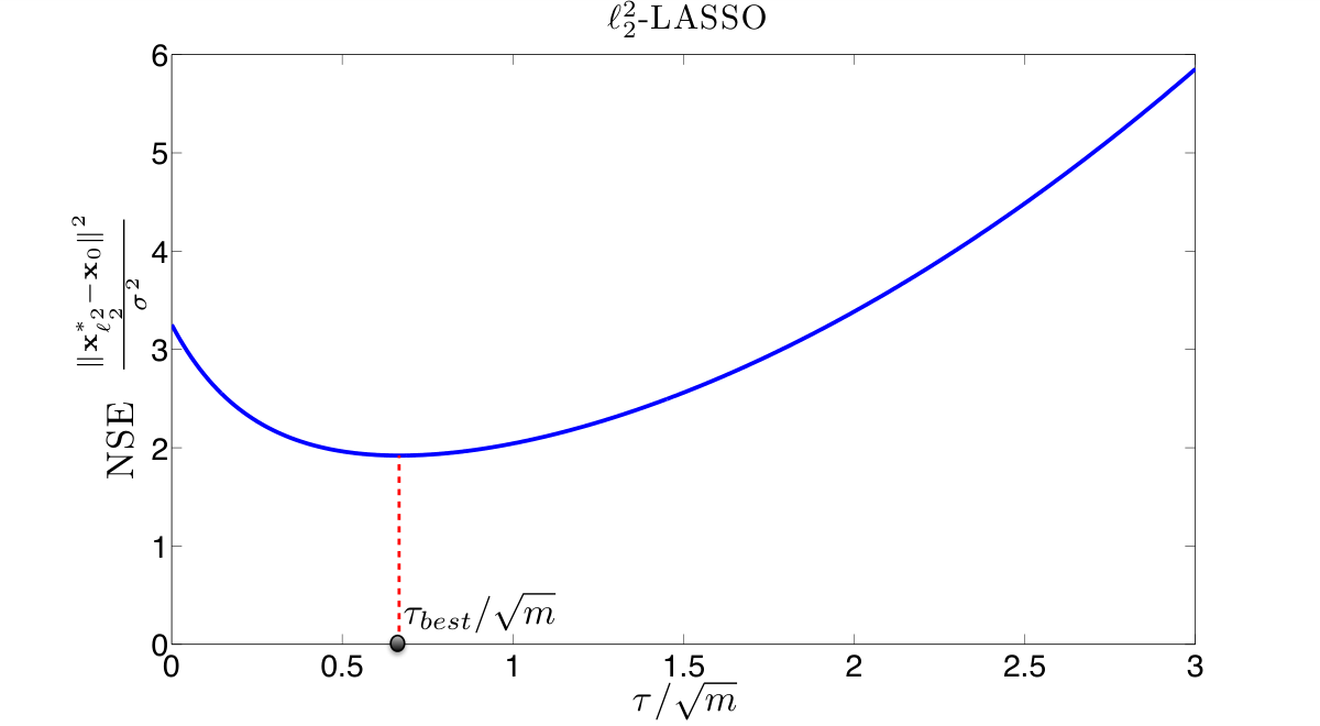
Figure 4: We consider the exact same setup of Figure 3. a) We plot m−𝐃f​(𝐱0,λ)m-{\mathbf{D}}_{f}(\mathbf{x}_{0},{\lambda}) and 𝐂f​(𝐱0,λ){\mathbf{C}}_{f}(\mathbf{x}_{0},{\lambda}) as a function of λ{\lambda} to illustrate the important penalty parameters λcrit,λbest,λmax\lambda_{\text{crit}},\lambda_{\text{best}},\lambda_{{\max}} and the regions of operation ℛOFF,ℛON,ℛ∞{\mathcal{R}}_{\text{OFF}},{\mathcal{R}}_{\text{ON}},{\mathcal{R}}_{\infty}. b) We plot the ℓ22\ell_{2}^{2}-LASSO error as a function of τm\frac{\tau}{\sqrt{m}} by using the map​(⋅){\text{map}}(\cdot) function. The normalization is due to the fact that τ\tau grows linearly in m\sqrt{m}.

4.3.3 A rule of thumb for the optimal penalty parameter

Formula 1 provides a simple recipe for computing the optimal value of the penalty parameter, which we call τb​e​s​t\tau_{{best}}. Recall that λbest\lambda_{\text{best}} minimizes the error in the ℓ2\ell_{2}-LASSO. Then, the proposed mapping between the two problems, suggests that τb​e​s​t=map​(λbest)\tau_{best}={\text{map}}(\lambda_{\text{best}}). To evaluate map​(λbest){\text{map}}(\lambda_{\text{best}}) we make use of Lemma 2.5 and the fact that d​𝐃f​(𝐱0,λ)d​λ=−2λ​𝐂f​(𝐱0,λ)\frac{d{\mathbf{D}}_{f}(\mathbf{x}_{0},{\lambda})}{d{\lambda}}=-\frac{2}{{\lambda}}{\mathbf{C}}_{f}(\mathbf{x}_{0},{\lambda}) for all λ≥0{\lambda}\geq 0. Combine this with the fact that λbest\lambda_{\text{best}} is the unique minimizer of 𝐃f​(𝐱0,λ){\mathbf{D}}_{f}(\mathbf{x}_{0},{\lambda}), to show that 𝐂f​(𝐱0,λbest)=0{\mathbf{C}}_{f}(\mathbf{x}_{0},\lambda_{\text{best}})=0, and to conclude with,

τbest=λbest​m−𝐃f​(𝐱0,λbest).\displaystyle\tau_{\text{best}}=\lambda_{\text{best}}\sqrt{m-{\mathbf{D}}_{f}(\mathbf{x}_{0},\lambda_{\text{best}})}. (4.4)

As a last comment, (4.4) simplifies even further if one uses the fact 𝐃f​(𝐱0,λbest)≈𝐃f​(𝐱0,ℝ+){\mathbf{D}}_{f}(\mathbf{x}_{0},\lambda_{\text{best}})\approx{\mathbf{D}}_{f}(\mathbf{x}_{0},{\mathbb{R}}^{+}), which is valid under reasonable assumptions, [32, 41, 31]. In this case, τb​e​s​t≈λbest​m−𝐃f​(𝐱0,ℝ+)\tau_{best}\approx\lambda_{\text{best}}\sqrt{m-{\mathbf{D}}_{f}(\mathbf{x}_{0},{\mathbb{R}}^{+})}.

4.4.   Closed Form Calculations of the Formulae

Normalized Squared Error
C-LASSO 𝐃f​(𝐱0,ℝ+)m−𝐃f​(𝐱0,ℝ+)\frac{{\mathbf{D}}_{f}(\mathbf{x}_{0},{\mathbb{R}}^{+})}{m-{\mathbf{D}}_{f}(\mathbf{x}_{0},{\mathbb{R}}^{+})}
ℓ2\ell_{2}-LASSO 𝐃f​(𝐱0,λ)m−𝐃f​(𝐱0,λ)\frac{{\mathbf{D}}_{f}(\mathbf{x}_{0},{\lambda})}{m-{\mathbf{D}}_{f}(\mathbf{x}_{0},{\lambda})} for λ∈ℛON{\lambda}\in{\mathcal{R}}_{\text{ON}}
ℓ22\ell_{2}^{2}-LASSO 𝐃f​(𝐱0,map−1​(τ))m−𝐃f​(𝐱0,map−1​(τ))\frac{{\mathbf{D}}_{f}(\mathbf{x}_{0},{\text{map}}^{-1}(\tau))}{m-{\mathbf{D}}_{f}(\mathbf{x}_{0},{\text{map}}^{-1}(\tau))} for τ∈ℝ+{\tau}\in\mathbb{R}^{+}
Table 2: Summary of formulae for the NSE.

Table 2 summarizes the formulae for the NSE of the three versions of the LASSO problem. While simple and concise, it may appear to the reader that the formulae are rather abstract, because of the presence of 𝐃f​(𝐱0,ℝ+){\mathbf{D}}_{f}(\mathbf{x}_{0},{\mathbb{R}}^{+}) and 𝐃f​(𝐱0,λ){\mathbf{D}}_{f}(\mathbf{x}_{0},{\lambda}) (𝐂f​(𝐱0,λ){\mathbf{C}}_{f}(\mathbf{x}_{0},{\lambda}) is also implicitly involved in the calculation of map−1​(⋅){\text{map}}^{-1}(\cdot)) which were introduced to capture the convex geometry of the problem. However, as discussed here, for certain critical regularizers f⁡(⋅)f(\cdot), one can calculate (tight) upper bounds or even explicit formulas for these quantities. For example, for the estimation of a kk-sparse signal 𝐱0\mathbf{x}_{0} with f(⋅)=∥⋅∥1f(\cdot)=\|\cdot\|_{1}, it has been shown that 𝐃f​(𝐱0,ℝ+)≲2​k​(log⁡nk+1){\mathbf{D}}_{f}(\mathbf{x}_{0},{\mathbb{R}}^{+})\lesssim 2k(\log\frac{n}{k}+1). Substituting this into the formula for the NSE of the C-LASSO results in the “closed-form" upper bound given in (1.9), i.e. one expressed only in terms of mm,nn and kk. Analogous results have been derived [25, 55, 48, 32] for other well-known signal models as well, including low rankness (see (1.10)) and block-sparsity (see (1.11)). The first row of Table 3 summarizes some of the results for 𝐃f​(𝐱0,ℝ+){\mathbf{D}}_{f}(\mathbf{x}_{0},{\mathbb{R}}^{+}) found in the literature (see [25, 32]). The second row provides our closed form results on 𝐃f​(𝐱0,λ){\mathbf{D}}_{f}(\mathbf{x}_{0},{\lambda}) when λ{\lambda} is sufficiently large. The reader will observe that, by setting λ{\lambda} to its lower bound in the second row, one approximately obtains the corresponding result in the first row. For a related discussion on 𝐃f​(𝐱0,λ){\mathbf{D}}_{f}(\mathbf{x}_{0},{\lambda}) and closed form bounds, the reader is referred to [32]. The derivation of these results can be found in Section H of the Appendix. In the same section, we also provide exact formulas for 𝐃f​(𝐱0,λ){\mathbf{D}}_{f}(\mathbf{x}_{0},{\lambda}) and 𝐂f​(𝐱0,λ){\mathbf{C}}_{f}(\mathbf{x}_{0},{\lambda}) for the same signal models. Based on those formulas and Table 3, one simply needs to substitute 𝐃f​(𝐱0,ℝ+){\mathbf{D}}_{f}(\mathbf{x}_{0},{\mathbb{R}}^{+}) or 𝐃f​(𝐱0,λ){\mathbf{D}}_{f}(\mathbf{x}_{0},{\lambda}) with their corresponding value to reach the error bounds. We should emphasize that, examples are not limited to the ones discussed here (see for instance [25]).

kk-sparse, 𝐱0∈ℝn\mathbf{x}_{0}\in\mathbb{R}^{n} Rank rr, 𝐗0∈ℝd×d\mathbf{X}_{0}\in\mathbb{R}^{d\times d} kk-block sparse, 𝐱0∈ℝt​b\mathbf{x}_{0}\in\mathbb{R}^{tb}
𝐃f​(𝐱0,ℝ+){\mathbf{D}}_{f}(\mathbf{x}_{0},{\mathbb{R}}^{+}) 2​k​(log⁡nk+1)2k(\log\frac{n}{k}+1) 6​d​r6dr 4​k​(log⁡tk+b)4k(\log\frac{t}{k}+b)
𝐃f​(𝐱0,λ){\mathbf{D}}_{f}(\mathbf{x}_{0},{\lambda}) (λ2+3)​k({\lambda}^{2}+3)k  for  λ≥2​log⁡nk{\lambda}\geq\sqrt{2\log\frac{n}{k}} λ2​r+2​d​(r+1){\lambda}^{2}r+2d(r+1)  for  λ≥2​d{\lambda}\geq 2\sqrt{d} (λ2+b+2)​k({\lambda}^{2}+b+2)k  for  λ≥b+2​log⁡tk{\lambda}\geq\sqrt{b}+\sqrt{2\log\frac{t}{k}}
Table 3: Closed form upper bounds for 𝐃f​(𝐱0,ℝ+){\mathbf{D}}_{f}(\mathbf{x}_{0},{\mathbb{R}}^{+}) ([25, 32]) and 𝐃f​(𝐱0,λ){\mathbf{D}}_{f}(\mathbf{x}_{0},{\lambda}) corresponding to (1.9), (1.10) and (1.11).

It follows from this discussion, that establishing new and tighter analytic bounds for 𝐃f​(𝐱0,λ){\mathbf{D}}_{f}(\mathbf{x}_{0},{\lambda}) and 𝐃f​(𝐱0,ℝ+){\mathbf{D}}_{f}(\mathbf{x}_{0},{\mathbb{R}}^{+}) for more regularizers ff is certainly an interesting direction for future research. In the case where such analytic bounds do not already exist in literature or are hard to derive, one can numerically estimate 𝐃f​(𝐱0,λ){\mathbf{D}}_{f}(\mathbf{x}_{0},{\lambda}) and 𝐃f​(𝐱0,ℝ+){\mathbf{D}}_{f}(\mathbf{x}_{0},{\mathbb{R}}^{+}) once there is an available characterization of the set of subdifferentials ∂f⁡(𝐱0)\partial f(\mathbf{x}_{0}). More in detail, it is not hard to show that, when 𝐡∼𝒩⁡(0,𝐈n)\mathbf{h}\sim\mathcal{N}(0,\mathbf{I}_{n}), dist2​(𝐡,λ​∂f⁡(𝐱0))\text{{dist}}^{2}(\mathbf{h},{\lambda}\partial f(\mathbf{x}_{0})) concentrates nicely around 𝐃f​(𝐱0,λ){\mathbf{D}}_{f}(\mathbf{x}_{0},{\lambda}) (see Lemma B.3) . Hence to compute 𝐃f​(𝐱0,λ){\mathbf{D}}_{f}(\mathbf{x}_{0},{\lambda}):

  1. (a)

    draw a vector 𝐡∼𝒩⁡(0,𝐈n)\mathbf{h}\sim\mathcal{N}(0,\mathbf{I}_{n}),

  2. (b)

    return the solution of the convex program min𝐬∈∂f⁡(𝐱0)⁡‖𝐡−λ​𝐬‖2\min_{\mathbf{s}\in\partial f(\mathbf{x}_{0})}{\|\mathbf{h}-{\lambda}\mathbf{s}\|^{2}}.

Computing 𝐃f​(𝐱0,ℝ+){\mathbf{D}}_{f}(\mathbf{x}_{0},{\mathbb{R}}^{+}) can be built on the same recipe by writing dist2​(𝐡,cone​(∂f⁡(𝐱0)))\text{{dist}}^{2}(\mathbf{h},\text{cone}(\partial f(\mathbf{x}_{0}))) as minλ≥0,𝐬∈∂f⁡(𝐱0)⁡‖𝐡−λ​𝐬‖2\min_{{\lambda}\geq 0,\mathbf{s}\in\partial f(\mathbf{x}_{0})}{\|\mathbf{h}-{\lambda}\mathbf{s}\|^{2}}.

Summing up, our proposed formulae for the NSE of the LASSO problems can be effectively calculated, either analytically or numerically.

4.5.   Translating the Results

Until this point, we have considered the scenario, in which the measurement matrix 𝐀\mathbf{A} has independent standard normal entries, and the noise vector 𝐳\mathbf{z} is equal to σ​𝐯\sigma\mathbf{v} with 𝐯∼𝒩⁡(0,𝐈m)\mathbf{v}\sim\mathcal{N}(0,\mathbf{I}_{m}). In related literature, the entries of 𝐀\mathbf{A} are often assumed to have variance 1m\frac{1}{m} or 1n\frac{1}{n}, [15, 14, 17]. For example, a variance of 1m\frac{1}{m} ensures that in expectation ‖𝐀𝐱‖2\|\mathbf{A}\mathbf{x}\|^{2} is same as ‖𝐱‖2\|\mathbf{x}\|^{2}. Hence, it is important to understand, how our setting can be translated to those. To distinguish our setup from the “non-unit variance” setup, we introduce the “non-unit variance” variables 𝐀′,σ′,λ′\mathbf{A}^{\prime},\sigma^{\prime},{\lambda}^{\prime} and τ′\tau^{\prime}. Let entries of 𝐀′\mathbf{A}^{\prime} have variance 1m\frac{1}{m} and consider the ℓ2\ell_{2}-LASSO problem with these new variables, which can be equivalently written as,

min𝐱⁡‖𝐀′​𝐱0+σ′​𝐯−𝐀′​𝐱‖+λ′​f​(𝐱).\min_{\mathbf{x}}\|\mathbf{A}^{\prime}\mathbf{x}_{0}+\sigma^{\prime}\mathbf{v}-\mathbf{A}^{\prime}\mathbf{x}\|+{\lambda}^{\prime}f(\mathbf{x}).

Multiplying the objective with m\sqrt{m}, we obtain,

min𝐱⁡‖m​𝐀′​𝐱0+m​σ′​𝐯−m​𝐀′​𝐱‖+m​λ′​f​(𝐱).\min_{\mathbf{x}}\|\sqrt{m}\mathbf{A}^{\prime}\mathbf{x}_{0}+\sqrt{m}\sigma^{\prime}\mathbf{v}-\sqrt{m}\mathbf{A}^{\prime}\mathbf{x}\|+\sqrt{m}{\lambda}^{\prime}f(\mathbf{x}).

Observe that, m​𝐀′\sqrt{m}\mathbf{A}^{\prime} is now statistically identical to 𝐀\mathbf{A}. Hence, Theorem 3.2 is applicable under the mapping σ←m​σ′\sigma\leftarrow\sqrt{m}\sigma^{\prime} and λ←m​λ′{\lambda}\leftarrow\sqrt{m}{\lambda}^{\prime}. Consequently, the NSE formula for the new setting for m​λ′∈ℛON\sqrt{m}{\lambda}^{\prime}\in{\mathcal{R}}_{\text{ON}} can be given as,

‖𝐱ℓ2∗−𝐱0‖2(m​σ′)2=‖𝐱ℓ2∗−𝐱0‖2σ2≲𝐃f​(𝐱0,λ)m−𝐃f​(𝐱0,λ)=𝐃f​(𝐱0,m​λ′)m−𝐃f​(𝐱0,m​λ′).\frac{\|\mathbf{x}^{*}_{\ell_{2}}-\mathbf{x}_{0}\|^{2}}{({\sqrt{m}\sigma^{\prime}})^{2}}=\frac{\|\mathbf{x}^{*}_{\ell_{2}}-\mathbf{x}_{0}\|^{2}}{{\sigma}^{2}}\lesssim\frac{{\mathbf{D}}_{f}(\mathbf{x}_{0},{\lambda})}{m-{\mathbf{D}}_{f}(\mathbf{x}_{0},{\lambda})}=\frac{{\mathbf{D}}_{f}(\mathbf{x}_{0},\sqrt{m}{\lambda}^{\prime})}{m-{\mathbf{D}}_{f}(\mathbf{x}_{0},\sqrt{m}{\lambda}^{\prime})}.

Identical arguments for the Constrained-LASSO and ℓ22\ell_{2}^{2}-LASSO results in the following NSE formulas,

‖𝐱c∗−𝐱0‖2m​σ′2≲𝐃f​(𝐱0,ℝ+)m−𝐃f​(𝐱0,ℝ+) and ‖𝐱ℓ22∗−𝐱0‖2m​σ′2≲𝐃f​(𝐱0,map−1​(m​τ′))m−𝐃f​(𝐱0,map−1​(m​τ′)).\frac{\|\mathbf{x}^{*}_{c}-\mathbf{x}_{0}\|^{2}}{m{\sigma^{\prime}}^{2}}\lesssim\frac{{\mathbf{D}}_{f}(\mathbf{x}_{0},{\mathbb{R}}^{+})}{m-{\mathbf{D}}_{f}(\mathbf{x}_{0},{\mathbb{R}}^{+})}\quad\text{ and }\quad\frac{\|\mathbf{x}^{*}_{\ell_{2}^{2}}-\mathbf{x}_{0}\|^{2}}{m{\sigma^{\prime}}^{2}}\lesssim\frac{{\mathbf{D}}_{f}(\mathbf{x}_{0},{\text{map}}^{-1}(m\tau^{\prime}))}{m-{\mathbf{D}}_{f}(\mathbf{x}_{0},{\text{map}}^{-1}(m\tau^{\prime}))}.

In general, reducing the signal power ‖𝐀𝐱0‖2\|\mathbf{A}\mathbf{x}_{0}\|^{2} by a factor of mm, amplifies the proposed NSE upper bound by mm times and the penalty parameters should be mapped as τ⟷m​τ′\tau\longleftrightarrow m\tau^{\prime} and λ⟷m​λ′{\lambda}\longleftrightarrow\sqrt{m}{\lambda}^{\prime}.

5. Applying Gordon’s Lemma

First, we introduce the basic notation that is used throughout the technical analysis of our results. Some additional notation, specific to the subject of each particular section is introduced later therein. To make explicit the variance of the noise vector 𝐳\mathbf{z}, we denote 𝐳=σ​𝐯\mathbf{z}=\sigma\mathbf{v}, where 𝐯∼𝒩⁡(0,𝐈m)\mathbf{v}\sim\mathcal{N}(0,\mathbf{I}_{m}). Also, we reserve the variables 𝐡\mathbf{h} and 𝐠\mathbf{g} to denote i.i.d. Gaussian vectors in 𝐑n\mathbf{R}^{n} and 𝐑m\mathbf{R}^{m}, respectively. In similar flavor, reserve the variable 𝐬\mathbf{s} to describe the subgradients of ff at 𝐱0\mathbf{x}_{0}. Finally, the Euclidean unit ball and unit sphere are respectively denoted as

ℬn−1:={𝐱∈ℝn|‖𝐱‖≤1} and 𝒮n−1:={𝐱∈ℝn|‖𝐱‖=1}.\displaystyle{\mathcal{B}}^{n-1}:=\left\{\mathbf{x}\in\mathbb{R}^{n}~|~\|\mathbf{x}\|\leq 1\right\}\quad\text{ and }\quad{\mathcal{S}}^{n-1}:=\left\{\mathbf{x}\in\mathbb{R}^{n}~|~\|\mathbf{x}\|=1\right\}.

5.1.   Introducing the Error Vector

For each candidate solution 𝐱\mathbf{x} of the LASSO algorithm, denote 𝐰=𝐱−𝐱0\mathbf{w}=\mathbf{x}-\mathbf{x}_{0}. Solving for 𝐰\mathbf{w} is clearly equivalent to solving for 𝐱\mathbf{x}, but simplifies considerably the presentation of the analysis. Under this notation, ‖𝐲−𝐀𝐱‖=‖𝐀𝐰−σ​𝐯‖.\|\mathbf{y}-\mathbf{A}\mathbf{x}\|=\|\mathbf{A}\mathbf{w}-\sigma\mathbf{v}\|. Furthermore, it is convenient to subtract the constant factor λ​f​(𝐱0){\lambda}f(\mathbf{x}_{0}) from the objective function of the LASSO problem and their approximations. In this direction, define the following “perturbation" functions:

fp​(𝐰)\displaystyle f_{p}(\mathbf{w}) =f⁡(𝐱0+𝐰)−f⁡(𝐱0),\displaystyle=f(\mathbf{x}_{0}+\mathbf{w})-f(\mathbf{x}_{0}), (5.1)
f^p​(𝐰)\displaystyle\hat{f}_{p}(\mathbf{w}) =f^​(𝐱0+𝐰)−f⁡(𝐱0)=sup𝐬∈∂f⁡(𝐱0)𝐬T​𝐰.\displaystyle=\hat{f}(\mathbf{x}_{0}+\mathbf{w})-f(\mathbf{x}_{0})=\sup_{\mathbf{s}\in\partial f(\mathbf{x}_{0})}\mathbf{s}^{T}\mathbf{w}. (5.2)

Then, the ℓ2\ell_{2}-LASSO will write as

𝐰ℓ2∗=arg⁡min𝐰​{‖𝐀𝐰−σ​𝐯‖+λ​fp​(𝐰)}.\displaystyle\mathbf{w}^{*}_{\ell_{2}}=\arg\min_{\mathbf{w}}\left\{\|\mathbf{A}\mathbf{w}-\sigma\mathbf{v}\|+{\lambda}f_{p}(\mathbf{w})\right\}. (5.3)

and the C-LASSO as

𝐰c∗=\displaystyle\mathbf{w}_{c}^{*}= arg⁡min𝐰​‖𝐀𝐰−σ​𝐯‖\displaystyle\arg\min_{\mathbf{w}}~\|\mathbf{A}\mathbf{w}-\sigma\mathbf{v}\|~
s.t.​fp​(𝐰)≤0.\displaystyle~~~~~~~\text{s.t.}~~~{f}_{p}(\mathbf{w})\leq 0.

or, equivalently,

𝐰c∗=arg⁡min𝐰​{‖𝐀𝐰−σ​𝐯‖+maxλ≥0⁡λ​fp​(𝐰)}.\displaystyle\mathbf{w}^{*}_{c}=\arg\min_{\mathbf{w}}\left\{~\|\mathbf{A}\mathbf{w}-\sigma\mathbf{v}\|+\max_{{\lambda}\geq 0}{\lambda}{f}_{p}(\mathbf{w})~\right\}. (5.4)

5.2.   The Approximate LASSO Problem

In Section 2, and in particular in (2.3) we introduced the approximated ℓ2\ell_{2}-LASSO problem. We repeat the definition here, and also, we define accordingly the approximate C-LASSO. The approximated ℓ2\ell_{2}-LASSO writes:

𝐰^ℓ2=arg⁡min𝐰​{‖𝐀𝐰−σ​𝐯‖+λ​f^p​(𝐰)}.\displaystyle\hat{\mathbf{w}}_{\ell_{2}}=\arg\min_{\mathbf{w}}\left\{\|\mathbf{A}\mathbf{w}-\sigma\mathbf{v}\|+{\lambda}\hat{f}_{p}(\mathbf{w})\right\}. (5.5)

Similarly, the approximated C-LASSO writes

𝐰^c=\displaystyle\hat{\mathbf{w}}_{c}~=~ arg⁡min𝐰​{‖𝐀𝐰−σ​𝐯‖+maxλ≥0⁡λ​f^p​(𝐰)}.\displaystyle\arg\min_{\mathbf{w}}\left\{~\|\mathbf{A}\mathbf{w}-\sigma\mathbf{v}\|+\max_{{\lambda}\geq 0}{\lambda}\hat{f}_{p}(\mathbf{w})~\right\}. (5.6)

Denote ℱ^c​(𝐀,𝐯)\hat{{\mathcal{F}}}_{c}(\mathbf{A},\mathbf{v}) and ℱ^ℓ​2​(𝐀,𝐯)\hat{{\mathcal{F}}}_{\ell 2}(\mathbf{A},\mathbf{v}) the optimal costs of problems (5.6) and (5.5), respectively. Note our convention to use the symbol “^~\hat{}~" over variables that are associated with the approximate problems. To distinguish, we use the symbol “∗~{}^{*}~" for the variables associated with the original problems.

5.3.   Technical Tool: Gordon’s Lemma

As already noted the most important technical ingredient underlying our analysis is a Lemma proved by Gordon in [72]; recall Lemma 2.1 in Section 2. In fact, Gordon’s key Lemma 2.1 is a Corollary of a more general theorem which establishes a probabilistic comparison between two centered Gaussian processes. The theorem was proved by Gordon in [73] and is stated below for completeness.

Theorem 5.1 (Gordon’s Theorem, [72]).

Let {Xi​j}\left\{X_{ij}\right\} and {Yi​j}\left\{Y_{ij}\right\}, 1≤i≤n1\leq i\leq n, 1≤j≤m1\leq j\leq m, be two centered Gaussian processes which satisfy the following inequalities for all choices of indices

  1. 1.

    𝔼⁡[Xi​j2]=𝔼⁡[Yi​j2]{\mathbb{E}}\left[X_{ij}^{2}\right]={\mathbb{E}}\left[Y_{ij}^{2}\right],

  2. 2.

    𝔼⁡[Xi​j​Xi​k]≥𝔼⁡[Yi​j​Yi​k]{\mathbb{E}}\left[X_{ij}X_{ik}\right]\geq{\mathbb{E}}\left[Y_{ij}Y_{ik}\right],

  3. 3.

    𝔼⁡[Xi​j​Xℓ​k]≤𝔼⁡[Yi​j​Yℓ​k]{\mathbb{E}}\left[X_{ij}X_{\ell k}\right]\leq{\mathbb{E}}\left[Y_{ij}Y_{\ell k}\right],  if i≠ℓi\neq\ell.

Then,

ℙ(∩i∪j[Yi​j≥λi​j])≥ℙ(∩i∪j[Xi​j≥λi​j]),{\mathbb{P}}\left(\cap_{i}\cup_{j}\left[Y_{ij}\geq\lambda_{ij}\right]\right)\geq{\mathbb{P}}\left(\cap_{i}\cup_{j}\left[X_{ij}\geq\lambda_{ij}\right]\right),

for all choices of λi​j∈𝐑\lambda_{ij}\in\mathbf{R}.

Application of Gordon’s Theorem 5.1 to specific Gaussian processes results in Gordon’s Lemma 2.1 [72]. In this work, we require a slightly modified version of this lemma, namely Lemma 5.1. The key idea is of course the same as in the original lemma, but the statement is modified to fit the setup of the current paper.

Lemma 5.1 (Modified Gordon’s Lemma).

Let 𝐆\mathbf{G}, 𝐠\mathbf{g}, 𝐡\mathbf{h} be defined as in Lemma 2.1 and let ψ⁡(⋅,⋅):ℝn×ℝm→ℝ\psi(\cdot,\cdot):\mathbb{R}^{n}\times\mathbb{R}^{m}\rightarrow\mathbb{R} . Also, let Φ1⊂ℝn\Phi_{1}\subset\mathbb{R}^{n} and Φ2⊂ℝm\Phi_{2}\subset\mathbb{R}^{m} such that either both Φ1\Phi_{1} and Φ2\Phi_{2} are compact or Φ1\Phi_{1} is arbitrary and Φ2\Phi_{2} is a scaled unit sphere. Then, for any c∈ℝc\in\mathbb{R}:

ℙ⁡(min𝐱∈Φ1⁡max𝐚∈Φ2​{𝐚T​𝐆𝐱−ψ⁡(𝐱,𝐚)}≥c)≥2​ℙ​(min𝐱∈Φ1⁡max𝐚∈Φ2​{‖𝐱​‖𝐠T​𝐚−‖​𝐚‖​𝐡T​𝐱−ψ⁡(𝐱,𝐚)}≥c)−1.\displaystyle{\mathbb{P}}\left(\min_{\mathbf{x}\in\Phi_{1}}~\max_{\mathbf{a}\in\Phi_{2}}~\left\{\mathbf{a}^{T}\mathbf{G}\mathbf{x}-\psi({\mathbf{x},\mathbf{a}})\right\}\geq c\right)\geq 2{\mathbb{P}}\left(\min_{\mathbf{x}\in\Phi_{1}}\max_{\mathbf{a}\in\Phi_{2}}\left\{\|\mathbf{x}\|\mathbf{g}^{T}\mathbf{a}-\|\mathbf{a}\|\mathbf{h}^{T}\mathbf{x}-\psi({\mathbf{x},\mathbf{a}})\right\}\geq c\right)-1.

The proof of Lemma 5.1 closely parallels the proof of Lemma 5.1 in [72]. We defer the proof to Section C in the Appendix.

5.4.   Simplifying the LASSO objective through Gordon’s Lemma

Section 2.6 introduced the technical framework. Key feature in this framework is the application of Gordon’s Lemma. In particular, we apply Gordon’s Lemma three times: once each for the purposes of the lower bound, the upper bound and the deviation analysis. Each application results in a corresponding simplified problem, which we call “key optimization". The analysis is carried out for that latter one as opposed to the original and more complex LASSO problem. In this Section, we show the details of applying Gordon’s Lemma and we identify the corresponding key optimizations. Later, in Section 6, we focus on the approximate LASSO problem and we show that in that case, the key optimizations are amenable to detailed analysis.

To avoid unnecessary repetitions, we treat the original and approximate versions of both the C-LASSO and the ℓ2\ell_{2}-LASSO, in a common framework, by defining the following problem:

ℱ⁡(𝐀,𝐯)=min𝐰⁡{‖𝐀𝐰−σ​𝐯‖+p⁡(𝐰)},\displaystyle\mathcal{F}(\mathbf{A},\mathbf{v})=\min_{\mathbf{w}}{\left\{~\|\mathbf{A}\mathbf{w}-\sigma\mathbf{v}\|+p(\mathbf{w})~\right\}}, (5.7)

where p:𝐑n→𝐑∪∞p:\mathbf{R}^{n}\rightarrow\mathbf{R}\cup\infty is a proper convex function [86]. Choose the penalty function p⁡(⋅)p(\cdot) in the generic formulation (5.7) accordingly to end up with (5.3), (5.4), (5.5) or (5.6). To retrieve (5.4) and (5.6), choose p⁡(𝐰)p(\mathbf{w}) as the indicator function of the sets {𝐰|fp​(𝐰)≤0}\left\{\mathbf{w}|f_{p}(\mathbf{w})\leq 0\right\} and {𝐰|f^p​(𝐰)≤0}\left\{\mathbf{w}|\hat{f}_{p}(\mathbf{w})\leq 0\right\} [83].

5.4.1 Lower Bound

The following corollary is a direct application of Lemma 5.1 to ℱ⁡(𝐀,𝐯)\mathcal{F}(\mathbf{A},\mathbf{v}) in (5.7).

Corollary 5.1.

Let 𝐠∼𝒩⁡(0,𝐈m)\mathbf{g}\sim\mathcal{N}(0,\mathbf{I}_{m}), 𝐡∼𝒩⁡(0,𝐈n)\mathbf{h}\sim\mathcal{N}(0,\mathbf{I}_{n}) and h∼𝒩⁡(0,1)h\sim\mathcal{N}(0,1) and assume all 𝐠,𝐡,h\mathbf{g},\mathbf{h},h are independently generated. Let

ℒ⁡(𝐠,𝐡)=min𝐰⁡{‖𝐰‖2+σ2​‖𝐠‖−𝐡T​𝐰+p⁡(𝐰)}.\displaystyle\mathcal{{L}}(\mathbf{g},\mathbf{h})=\min_{\mathbf{w}}\left\{\sqrt{\|\mathbf{w}\|^{2}+\sigma^{2}}\|\mathbf{g}\|-\mathbf{h}^{T}\mathbf{w}+p(\mathbf{w})\right\}. (5.8)

Then, for any c∈ℝc\in\mathbb{R}:

ℙ⁡(ℱ⁡(𝐀,𝐯)≥c)≥2⋅ℙ⁡(ℒ⁡(𝐠,𝐡)−h​σ≥c)−1.\displaystyle{\mathbb{P}}\left(~\mathcal{F}(\mathbf{A},\mathbf{v})\geq c~\right)\geq 2\cdot{\mathbb{P}}\left(~\mathcal{{L}}(\mathbf{g},\mathbf{h})-h\sigma\geq c~\right)-1.
Proof.

Notice that ‖𝐀𝐰−σ​𝐯‖=‖𝐀𝐯​𝐰σ‖\|\mathbf{A}\mathbf{w}-\sigma\mathbf{v}\|=\|\mathbf{A}_{\mathbf{v}}\mathbf{w}_{\sigma}\|, where 𝐀𝐯:=[𝐀−𝐯]\mathbf{A}_{\mathbf{v}}:=[\mathbf{A}\ -\mathbf{v}] is a matrix with i.i.d. standard normal entries of size m×(n+1)m\times(n+1) and 𝐰σ=[𝐰T​σ]T∈ℝn+1\mathbf{w}_{\sigma}=[\mathbf{w}^{T}~\sigma]^{T}\in\mathbb{R}^{n+1}. Apply the modified Gordon’s Lemma 5.1, with 𝐱=𝐰σ\mathbf{x}=\mathbf{w}_{\sigma}, Φ1={𝐰σ|𝐰∈ℝn}\Phi_{1}=\{\mathbf{w}_{\sigma}\big|\mathbf{w}\in\mathbb{R}^{n}\}, Φ2=𝒮m−1\Phi_{2}=\mathcal{S}^{m-1}, 𝐆=𝐀𝐯\mathbf{G}=\mathbf{A}_{\mathbf{v}}, ψ⁡(𝐰σ)=p⁡(𝐰)\psi(\mathbf{w}_{\sigma})=p(\mathbf{w}). Further perform the trivial optimizations over 𝐚\mathbf{a} on both sides of the inequality. Namely, max‖𝐚‖=1⁡𝐚T​𝐀𝐳​[𝐰T​σ]T=‖𝐀𝐳​𝐰σ‖\max_{\|\mathbf{a}\|=1}\mathbf{a}^{T}\mathbf{A}_{\mathbf{z}}[\mathbf{w}^{T}~\sigma]^{T}=\|\mathbf{A}_{\mathbf{z}}\mathbf{w}_{\sigma}\| and, max‖𝐚‖=1⁡𝐠T​𝐚=‖𝐠‖\max_{\|\mathbf{a}\|=1}\mathbf{g}^{T}\mathbf{a}=\|\mathbf{g}\|. ∎

5.4.2 Upper Bound

Similar to the lower bound derived in the previous section, we derive an upper bound for ℱ⁡(𝐀,𝐯)\mathcal{F}(\mathbf{A},\mathbf{v}). For this, we need to apply Gordon’s Lemma to −ℱ⁡(𝐀,𝐯)-\mathcal{F}(\mathbf{A},\mathbf{v}) and use the dual formulation of it. Lemma D in the Appendix shows that the dual of the minimization in (5.7) can be written as

−ℱ⁡(𝐀,𝐯)=min‖𝝁‖≤1⁡max𝐰​{𝝁T​(𝐀𝐰−σ​𝐯)−p⁡(𝐰)}.\displaystyle-\mathcal{F}(\mathbf{A},\mathbf{v})=\min_{\|\bm{\mu}\|\leq 1}\max_{\mathbf{w}}\left\{\bm{\mu}^{T}\left(\mathbf{A}\mathbf{w}-\sigma\mathbf{v}\right)-p(\mathbf{w})\right\}. (5.9)

Lemma 5.1 requires the set over which maximization is performed to be compact. We thus apply Lemma 5.1 to the restricted problem,

min‖𝝁‖≤1⁡max‖𝐰‖≤Cu​p​{𝝁T​(𝐀𝐰−σ​𝐯)−p⁡(𝐰)}.\min_{\|\bm{\mu}\|\leq 1}~\max_{\|\mathbf{w}\|\leq C_{up}}\left\{\bm{\mu}^{T}\left(\mathbf{A}\mathbf{w}-\sigma\mathbf{v}\right)-p(\mathbf{w})\right\}.

Notice, that this still gives a valid lower bound to −ℱ⁡(𝐀,𝐯)-\mathcal{F}(\mathbf{A},\mathbf{v}) since the optimal cost of this latter problem is no larger than −ℱ⁡(𝐀,𝐯)-\mathcal{F}(\mathbf{A},\mathbf{v}). In Section 6, we will choose Cu​pC_{up} so that the resulting lower bound is as tight as possible.

Corollary 5.2.

Let 𝐠∼𝒩⁡(0,𝐈m)\mathbf{g}\sim\mathcal{N}(0,\mathbf{I}_{m}), 𝐡∼𝒩⁡(0,𝐈n)\mathbf{h}\sim\mathcal{N}(0,\mathbf{I}_{n}) and h∼𝒩⁡(0,1)h\sim\mathcal{N}(0,1) and assume all 𝐠,𝐡,h\mathbf{g},\mathbf{h},h are independently generated. Let,

𝒰⁡(𝐠,𝐡)=−min‖𝝁‖≤1⁡max‖𝐰‖≤Cu​p​{‖𝐰‖2+σ2​𝐠T​𝝁+‖𝝁‖​𝐡T​𝐰−p⁡(𝐰)}.\displaystyle\mathcal{{U}}(\mathbf{g},\mathbf{h})=-\min_{\|\bm{\mu}\|\leq 1}~\max_{\|\mathbf{w}\|\leq C_{up}}\left\{\sqrt{\|\mathbf{w}\|^{2}+\sigma^{2}}~\mathbf{g}^{T}\bm{\mu}+\|\bm{\mu}\|\mathbf{h}^{T}\mathbf{w}-p(\mathbf{w})\right\}. (5.10)

Then, for any c∈ℝc\in\mathbb{R}:

ℙ⁡(ℱ⁡(𝐀,𝐯)≤c)≥2⋅ℙ⁡(𝒰⁡(𝐠,𝐡)−min0≤α≤1⁡α​σ​h≤c)−1.\displaystyle{\mathbb{P}}\left(~\mathcal{F}(\mathbf{A},\mathbf{v})\leq c~\right)\geq 2\cdot{\mathbb{P}}\left(~\mathcal{{U}}(\mathbf{g},\mathbf{h})-\min_{0\leq\alpha\leq 1}\alpha\sigma h\leq c~\right)-1.
Proof.

Similar to the proof of Corollary 5.1 write ‖σ​𝐯−𝐀𝐰‖=‖𝐀𝐯​𝐰σ‖\|{\sigma}\mathbf{v}-\mathbf{A}\mathbf{w}\|=\|\mathbf{A}_{\mathbf{v}}\mathbf{w}_{\sigma}\|. Then, apply the modified Gordon’s Lemma 5.1, with 𝐱=𝝁\mathbf{x}=\bm{\mu}, α=𝐰σ\alpha=\mathbf{w}_{\sigma}, Φ1=ℬm−1\Phi_{1}=\mathcal{B}^{m-1}, Φ2={𝐰σ|1Cu​p​𝐰∈ℬn−1}\Phi_{2}=\left\{\mathbf{w}_{\sigma}~|~\frac{1}{C_{up}}\mathbf{w}\in{\mathcal{B}}^{n-1}\right\}, 𝐆=𝐀𝐯\mathbf{G}=\mathbf{A}_{\mathbf{v}}, ψ⁡(𝐰σ)=p⁡(𝐰)\psi(\mathbf{w}_{\sigma})=p(\mathbf{w}), to find that for any c∈ℝc\in\mathbb{R}:

ℙ⁡(−ℱ⁡(𝐀,𝐯)≥−c)\displaystyle{\mathbb{P}}\left(~-\mathcal{F}(\mathbf{A},\mathbf{v})\geq-c~\right) ≥2⋅ℙ⁡(min‖𝝁‖≤1⁡max‖𝐰‖≤Cu​p​{Cu​p2+σ2​𝐠T​𝝁+‖𝝁‖​𝐡T​𝐰−p⁡(𝐰)+‖𝝁‖​σ​h}≥−c)−1\displaystyle\geq 2\cdot{\mathbb{P}}\left(~\min_{\|\bm{\mu}\|\leq 1}~\max_{\|\mathbf{w}\|\leq C_{up}}\left\{\sqrt{C_{up}^{2}+\sigma^{2}}~\mathbf{g}^{T}\bm{\mu}+\|\bm{\mu}\|\mathbf{h}^{T}\mathbf{w}-p(\mathbf{w})+\|\bm{\mu}\|\sigma h\right\}\geq-c~\right)-1
≥2​ℙ​(−𝒰⁡(𝐠,𝐡)+min‖μ‖≤1⁡‖𝝁‖​σ​h≥−c)−1.\displaystyle\geq 2{\mathbb{P}}\left(~-\mathcal{{U}}(\mathbf{g},\mathbf{h})+\min_{\|\mu\|\leq 1}\|\bm{\mu}\|\sigma h\geq-c~\right)-1.

∎

5.4.3 Deviation Analysis

Of interest in the deviation analysis of the LASSO problem (cf. Step 4 in Section 2.6) is the analysis of a restricted version of the L​A​S​S​OLASSO problem, namely

min‖𝐰‖∈Sd​e​v⁡{‖𝐀𝐰−σ​𝐯‖+p⁡(𝐰)}\displaystyle\min_{\|\mathbf{w}\|\in S_{dev}}~\left\{\|\mathbf{A}\mathbf{w}-\sigma\mathbf{v}\|+p(\mathbf{w})\right\} (5.11)

where

Sd​e​v:={ℓ||ℓCd​e​v−1|≥δd​e​v}.S_{dev}:=\left\{\ell~|~\left|\frac{\ell}{C_{dev}}-1\right|\geq\delta_{dev}\right\}.

δd​e​v>0\delta_{dev}>0 is any arbitrary small constant and Cd​e​v>0C_{dev}>0 a constant that will be chosen carefully for the purpose of the deviation analysis . We establish a high probability lower bound for (5.11). As usual, we apply Lemma 5.1 to our setup, to conclude the following.

Corollary 5.3.

Let 𝐠∼𝒩⁡(0,𝐈m)\mathbf{g}\sim\mathcal{N}(0,\mathbf{I}_{m}), 𝐡∼𝒩⁡(0,𝐈n)\mathbf{h}\sim\mathcal{N}(0,\mathbf{I}_{n}) and h∼𝒩⁡(0,1)h\sim\mathcal{N}(0,1) and assume all 𝐠,𝐡,h\mathbf{g},\mathbf{h},h are independently generated. Let

ℒd​e​v​(𝐠,𝐡)=min‖𝐰‖∈Sd​e​v⁡{‖𝐰‖2+σ2​‖𝐠‖−𝐡T​𝐰+p⁡(𝐰)}.\displaystyle\mathcal{{L}}_{dev}(\mathbf{g},\mathbf{h})=\min_{\|\mathbf{w}\|\in S_{dev}}\left\{\sqrt{\|\mathbf{w}\|^{2}+\sigma^{2}}\|\mathbf{g}\|-\mathbf{h}^{T}\mathbf{w}+p(\mathbf{w})\right\}. (5.12)

Then, for any c∈ℝc\in\mathbb{R}:

ℙ⁡(min‖𝐰‖∈Sd​e​v⁡{‖𝐀𝐰−σ​𝐯‖+p⁡(𝐰)}≥c)≥2⋅ℙ⁡(ℒd​e​v​(𝐠,𝐡)−h​σ≥c)−1.\displaystyle{\mathbb{P}}\left(~\min_{\|\mathbf{w}\|\in S_{dev}}~\left\{\|\mathbf{A}\mathbf{w}-\sigma\mathbf{v}\|+p(\mathbf{w})\right\}\geq c~\right)\geq 2\cdot{\mathbb{P}}\left(~\mathcal{{L}}_{dev}(\mathbf{g},\mathbf{h})-h\sigma\geq c~\right)-1.
Proof.

Follows from Lemma 5.1 following exactly the same steps as in the proof of Corollary 5.1. ∎

The reader will observe that ℒ\mathcal{{L}} is a special case of ℒd​e​v\mathcal{{L}}_{dev} where Sd​e​v=ℝ+S_{dev}=\mathbb{R}^{+}.

5.4.4 Summary

We summarize the results of Corollaries 5.1, 5.2 and 5.3 in Lemma 5.2. Adding to a simple summary, we perform a further simplification of the corresponding statements. In particular, we discard the “distracting" term σ​h\sigma h in Corollaries 5.1 and 5.3, as well as the term min0≤α≤1⁡α​σ​h\min_{0\leq\alpha\leq 1}\alpha\sigma h in Corollary 5.2. Recall the definitions of the key optimizations ℒ\mathcal{{L}}, 𝒰\mathcal{{U}} and ℒd​e​v\mathcal{{L}}_{dev} in (5.8), (5.10) and (5.12).

Lemma 5.2.

Let 𝐠∼𝒩⁡(0,𝐈m)\mathbf{g}\sim\mathcal{N}(0,{\bf{I}}_{m}) and 𝐡∼𝒩⁡(0,𝐈n)\mathbf{h}\sim\mathcal{N}(0,{\bf{I}}_{n}) be independently generated. Then, for any positive constant ϵ>0\epsilon>0, the following are true:

1. ​ℙ​(ℱ⁡(𝐀,𝐯)≥c)≥2​ℙ​(ℒ⁡(𝐠,𝐡)−σ​ϵ​m≥c)−4​exp⁡(−ϵ2​m2)−1.\displaystyle\text{1.~~}{\mathbb{P}}\left(~\mathcal{F}(\mathbf{A},\mathbf{v})\geq c~\right)\geq 2~{\mathbb{P}}\left(~\mathcal{{L}}(\mathbf{g},\mathbf{h})-\sigma\epsilon\sqrt{m}\geq c~\right)-4\exp\left(-\frac{\epsilon^{2}m}{2}\right)-1.
2. ​ℙ​(ℱ⁡(𝐀,𝐯)≤c)≥2​ℙ​(𝒰⁡(𝐠,𝐡)+σ​ϵ​m≤c)−4​exp⁡(−ϵ2​m2)−1.\displaystyle\text{2.~~}{\mathbb{P}}\left(~\mathcal{F}(\mathbf{A},\mathbf{v})\leq c~\right)\geq 2~{\mathbb{P}}\left(~\mathcal{{U}}(\mathbf{g},\mathbf{h})+\sigma\epsilon\sqrt{m}\leq c~\right)-4\exp\left(-\frac{\epsilon^{2}m}{2}\right)-1.
3. ​ℙ​(min‖𝐰‖∈Sd​e​v⁡{‖𝐀𝐰−σ​𝐯‖+p⁡(𝐰)}≥c)≥2​ℙ​(ℒd​e​v​(𝐠,𝐡)−σ​ϵ​m≥c)−4​exp⁡(−ϵ2​m2)−1.\displaystyle\text{3.~~}{\mathbb{P}}\left(~\min_{\|\mathbf{w}\|\in S_{dev}}~\left\{\|\mathbf{A}\mathbf{w}-\sigma\mathbf{v}\|+p(\mathbf{w})\right\}\geq c~\right)\geq 2~{\mathbb{P}}\left(~\mathcal{{L}}_{dev}(\mathbf{g},\mathbf{h})-\sigma\epsilon\sqrt{m}\geq c~\right)-4\exp\left(-\frac{\epsilon^{2}m}{2}\right)-1.
Proof.

For h∼𝒩⁡(0,1)h\sim\mathcal{N}(0,1) and all ϵ>0\epsilon>0,

ℙ⁡(|h|≤ϵ​m)≥1−2​exp⁡(−ϵ2​m2).\displaystyle{\mathbb{P}}\left(|h|\leq\epsilon\sqrt{m}\right)\geq 1-2\exp(-\frac{\epsilon^{2}m}{2}). (5.13)

Thus,

ℙ⁡(ℒ⁡(𝐠,𝐡)−h​σ≥c)\displaystyle{\mathbb{P}}\left(~\mathcal{{L}}(\mathbf{g},\mathbf{h})-h\sigma\geq c~\right) ≥ℙ(ℒ(𝐠,𝐡)−ϵσm≥c,h≤ϵm)\displaystyle\geq{\mathbb{P}}\left(\mathcal{{L}}(\mathbf{g},\mathbf{h})-\epsilon\sigma\sqrt{m}\geq c~,~h\leq\epsilon\sqrt{m}~\right)
≥ℙ⁡(ℒ⁡(𝐠,𝐡)−ϵ​σ​m≥c)−2​exp⁡(−ϵ2​m2).\displaystyle\geq{\mathbb{P}}(\mathcal{{L}}(\mathbf{g},\mathbf{h})-\epsilon\sigma\sqrt{m}\geq c)-2\exp(-\frac{\epsilon^{2}m}{2}).

Combine this with Corollary 5.1 to conclude with the first statement of Lemma 5.2. The proof of the third statement of the Lemma follows the exact same steps applied this time to Corollary 5.3. For the second statement write,

ℙ⁡(𝒰⁡(𝐠,𝐡)−min‖μ‖≤1⁡‖𝝁‖​σ​h≤c)\displaystyle{\mathbb{P}}\left(~\mathcal{{U}}(\mathbf{g},\mathbf{h})-\min_{\|\mu\|\leq 1}\|\bm{\mu}\|\sigma h\leq c~\right) ≥ℙ⁡(𝒰⁡(𝐠,𝐡)+σ​|h|≤c)\displaystyle\geq{\mathbb{P}}\left(~\mathcal{{U}}(\mathbf{g},\mathbf{h})+\sigma|h|\leq c~\right)
≥ℙ(𝒰(𝐠,𝐡)+ϵσm≤c,|h|≤ϵm),\displaystyle\geq{\mathbb{P}}\left(~\mathcal{{U}}(\mathbf{g},\mathbf{h})+\epsilon\sigma\sqrt{m}\leq c~,~|h|\leq\epsilon\sqrt{m}~\right),

and use (5.13) as above. To conclude, combine with the statement of Corollary 5.2. ∎

6. After Gordon’s Lemma: Analyzing the Key Optimizations

6.1.   Preliminaries

This Section is devoted to the analysis of the three key optimizations introduced in the previous section. In particular, we focus on the approximated C-LASSO and ℓ2\ell_{2}-LASSO problems, for which a detailed such analysis is tractable. Recall that the approximated C-LASSO and ℓ2\ell_{2}-LASSO are obtained from the generic optimization in (5.7) when substituting p⁡(𝐰)=maxλ≥0⁡max𝐬∈λ​∂f⁡(𝐱0)​𝐬T​𝐰=max𝐬∈cone​(∂f⁡(𝐱0))⁡𝐬T​𝐰p(\mathbf{w})=\max_{{\lambda}\geq 0}\max_{\mathbf{s}\in{\lambda}\partial f(\mathbf{x}_{0})}\mathbf{s}^{T}\mathbf{w}=\max_{\mathbf{s}\in\text{cone}(\partial f(\mathbf{x}_{0}))}\mathbf{s}^{T}\mathbf{w} and p⁡(𝐰)=max𝐬∈λ​∂f⁡(𝐱0)⁡𝐬T​𝐰p(\mathbf{w})=\max_{\mathbf{s}\in{\lambda}\partial f(\mathbf{x}_{0})}\mathbf{s}^{T}\mathbf{w}, respectively. Considering this and recalling the definitions in (5.8), (5.10) and (5.12), we will be analyzing the following key optimizations,

ℒ^​(𝐠,𝐡)\displaystyle\hat{\mathcal{L}}(\mathbf{g},\mathbf{h}) =min𝐰⁡{‖𝐰‖2+σ2​‖𝐠‖−𝐡T​𝐰+max𝐬∈𝒞⁡𝐬T​𝐰},\displaystyle=\min_{\mathbf{w}}\left\{\sqrt{\|\mathbf{w}\|^{2}+\sigma^{2}}\|\mathbf{g}\|-\mathbf{h}^{T}\mathbf{w}+\max_{\mathbf{s}\in\mathcal{C}}\mathbf{s}^{T}\mathbf{w}\right\}, (6.1a)
𝒰^​(𝐠,𝐡)\displaystyle\hat{\mathcal{U}}(\mathbf{g},\mathbf{h}) =−min‖𝝁‖≤1⁡max‖𝐰‖=Cu​p​{‖𝐰‖2+σ2​𝐠T​𝝁+‖𝝁‖​𝐡T​𝐰−max𝐬∈𝒞⁡𝐬T​𝐰},\displaystyle=-\min_{\|\bm{\mu}\|\leq 1}~\max_{\|\mathbf{w}\|=C_{up}}\left\{\sqrt{\|\mathbf{w}\|^{2}+\sigma^{2}}~\mathbf{g}^{T}\bm{\mu}+\|\bm{\mu}\|\mathbf{h}^{T}\mathbf{w}-\max_{\mathbf{s}\in\mathcal{C}}\mathbf{s}^{T}\mathbf{w}\right\}, (6.1b)
ℒ^d​e​v​(𝐠,𝐡)\displaystyle\hat{\mathcal{L}}_{dev}(\mathbf{g},\mathbf{h}) =min‖𝐰‖∈Sd​e​v⁡{‖𝐰‖2+σ2​‖𝐠‖−𝐡T​𝐰+max𝐬∈𝒞⁡𝐬T​𝐰},\displaystyle=\min_{\|\mathbf{w}\|\in S_{dev}}\left\{\sqrt{\|\mathbf{w}\|^{2}+\sigma^{2}}\|\mathbf{g}\|-\mathbf{h}^{T}\mathbf{w}+\max_{\mathbf{s}\in\mathcal{C}}\mathbf{s}^{T}\mathbf{w}\right\}, (6.1c)

where 𝒞\mathcal{C} is taken to be either cone​(∂f​(𝐱0))\text{cone}(\partial f(\mathbf{x}_{0})) or λ​∂f⁡(𝐱0){\lambda}\partial f(\mathbf{x}_{0}), corresponding to the C-LASSO and ℓ2\ell_{2}-LASSO, respectively. Notice that in (6.1b) we have constrained the feasible set of the inner maximization to the scaled sphere rather than ball. Following our discussion, in Section 5.4.2 this does not affect the validity of Lemma 5.2, while it facilitates our derivations here.

To be consistent with the definitions in (6.1), which treat the key optimizations of the C-LASSO and ℓ2\ell_{2}-LASSO under a common framework with introducing a generic set 𝒞\mathcal{C}, we also define

ℱ^​(𝐀,𝐯)=min𝐰⁡{‖𝐀𝐰−σ​𝐯‖+max𝐬∈𝒞⁡𝐬T​𝐰},\displaystyle\hat{{\mathcal{F}}}(\mathbf{A},\mathbf{v})=\min_{\mathbf{w}}\left\{\|\mathbf{A}\mathbf{w}-\sigma\mathbf{v}\|+\max_{\mathbf{s}\in\mathcal{C}}\mathbf{s}^{T}\mathbf{w}\right\}, (6.2)

to correspond to (5.6) and (5.5), when setting 𝒞=cone​(∂f⁡(𝐱0))\mathcal{C}=\text{cone}(\partial f(\mathbf{x}_{0})) and 𝒞=λ​∂f⁡(𝐱0)\mathcal{C}={\lambda}\partial f(\mathbf{x}_{0}), respectively.

6.2.   Some Notation

Let 𝒞⊂ℝn\mathcal{C}\subset\mathbb{R}^{n} be a closed and nonempty convex set. For any vector 𝐱∈ℝn\mathbf{x}\in\mathbb{R}^{n}, we denote its (unique) projection onto 𝒞\mathcal{C} as Proj​(𝐱,𝒞)\text{Proj}(\mathbf{x},\mathcal{C}), i.e.

Proj​(𝐱,𝒞):=argmin𝐬∈𝒞⁡‖𝐱−𝐬‖.\text{Proj}(\mathbf{x},\mathcal{C}):=\operatorname{argmin}_{\mathbf{s}\in\mathcal{C}}{\|\mathbf{x}-\mathbf{s}\|}.

It will also be convenient to denote,

Π⁡(𝐱,𝒞):=𝐱−Proj​(𝐱,𝒞).{\Pi}(\mathbf{x},\mathcal{C}):=\mathbf{x}-\text{Proj}(\mathbf{x},\mathcal{C}).

The distance of 𝐱\mathbf{x} to the set 𝒞\mathcal{C} can then be written as,

dist​(𝐱,𝒞):=‖Π​(𝐱,𝒞)‖.\text{{dist}}(\mathbf{x},\mathcal{C}):=\|{\Pi}(\mathbf{x},\mathcal{C})\|.

Finally, we denote,

corr​(𝐱,𝒞):=⟨Proj​(𝐱,𝒞),Π⁡(𝐱,𝒞)⟩.\text{corr}(\mathbf{x},\mathcal{C}):=\left<\text{Proj}(\mathbf{x},\mathcal{C}),{\Pi}(\mathbf{x},\mathcal{C})\right>.

Now, let 𝐡∼𝒩⁡(0,𝐈n)\mathbf{h}\sim\mathcal{N}(0,\mathbf{I}_{n}). The following quantities are of central interest throughout the paper:

𝐃⁡(𝒞)\displaystyle{\mathbf{D}}(\mathcal{C}) :=𝔼⁡[dist2​(𝐡,𝒞)],\displaystyle:={\mathbb{E}}\left[~\text{{dist}}^{2}(\mathbf{h},\mathcal{C})~\right], (6.3a)
𝐏⁡(𝒞)\displaystyle{\mathbf{P}}(\mathcal{C}) :=𝔼⁡[‖Proj​(𝐡,𝒞)‖2],\displaystyle:={\mathbb{E}}\left[~\|\text{Proj}(\mathbf{h},\mathcal{C})\|^{2}~\right], (6.3b)
𝐂⁡(𝒞)\displaystyle{\mathbf{C}}(\mathcal{C}) :=𝔼​[corr​(𝐡,𝒞)],\displaystyle:={\mathbb{E}}\left[~\text{corr}(\mathbf{h},\mathcal{C})~\right], (6.3c)

where the 𝔼⁡[⋅]{\mathbb{E}}[\cdot] is over the distribution of the Gaussian vector 𝐡\mathbf{h}. It is easy to verify that n=𝐃⁡(𝒞)+𝐏⁡(𝒞)+2​𝐂​(𝒞).n={\mathbf{D}}(\mathcal{C})+{\mathbf{P}}(\mathcal{C})+2{\mathbf{C}}(\mathcal{C}). Under this notation,

𝐃f​(𝐱0,λ)\displaystyle{\mathbf{D}}_{f}(\mathbf{x}_{0},{\lambda}) =𝐃⁡(λ​∂f⁡(𝐱0)),\displaystyle=\mathbf{D}({\lambda}\partial f(\mathbf{x}_{0})),
𝐂f​(𝐱0,λ)\displaystyle{\mathbf{C}}_{f}(\mathbf{x}_{0},{\lambda}) =𝐂⁡(λ​∂f⁡(𝐱0)),\displaystyle=\mathbf{C}({\lambda}\partial f(\mathbf{x}_{0})),
𝐃f​(𝐱0,ℝ+)\displaystyle{\mathbf{D}}_{f}(\mathbf{x}_{0},{\mathbb{R}}^{+}) =𝐃⁡(cone​(∂f⁡(𝐱0))).\displaystyle=\mathbf{D}(\text{cone}(\partial f(\mathbf{x}_{0}))).

On the same lines, define 𝐏f​(𝐱0,λ):=𝐏⁡(λ​∂f⁡(𝐱0)){\mathbf{P}}_{f}(\mathbf{x}_{0},{\lambda}):=\mathbf{P}({\lambda}\partial f(\mathbf{x}_{0})).

6.3.   Analysis

We perform a detailed analysis of the three key optimization problems ℒ^\hat{\mathcal{L}}, 𝒰^\hat{\mathcal{U}} and ℒ^d​e​v\hat{\mathcal{L}}_{dev}. For each one of them we summarize the results of the analysis in Lemmas 6.1, 6.2 and 6.3 below. Each Lemma includes three statements. In the first, we reduce the corresponding key optimization problem to a scalar optimization. Next, we compute the optimal value of this optimization in a deterministic setup. We convert this into a probabilistic statement in the last step, which is directly applicable in Lemma 5.2. Eventhough, we are eventually interested only in this last probabilistic statement, we have decided to include all three steps in the statement of the Lemmas in order to provide some further intuition into how they nicely build up to the desired result. All proofs of the lemmas are deferred to Section E in the Appendix.

6.3.1 Lower Key Optimization

Lemma 6.1 (Properties of ℒ^\hat{\mathcal{L}}).

Let 𝐠∼𝒩⁡(0,𝐈m)\mathbf{g}\sim\mathcal{N}(0,\mathbf{I}_{m}) and 𝐡∼𝒩⁡(0,𝐈n)\mathbf{h}\sim\mathcal{N}(0,\mathbf{I}_{n}) and

ℒ^​(𝐠,𝐡)=min𝐰⁡{‖𝐰‖2+σ2​‖𝐠‖−𝐡T​𝐰+max𝐬∈𝒞⁡𝐬T​𝐰},\displaystyle\hat{\mathcal{L}}(\mathbf{g},\mathbf{h})=\min_{\mathbf{w}}\left\{\sqrt{\|\mathbf{w}\|^{2}+\sigma^{2}}\|\mathbf{g}\|-\mathbf{h}^{T}\mathbf{w}+\max_{\mathbf{s}\in\mathcal{C}}\mathbf{s}^{T}\mathbf{w}\right\}, (6.4)

Denote 𝐰^l​o​w​(𝐠,𝐡)\hat{\mathbf{w}}_{low}(\mathbf{g},\mathbf{h}) its optimal value. The following are true:

  1. 1.

    Scalarization: ℒ^​(𝐠,𝐡)=minα≥0⁡{α2+σ2​‖𝐠‖−α⋅dist​(𝐡,𝒞)}\hat{\mathcal{L}}(\mathbf{g},\mathbf{h})=\min_{\alpha\geq 0}\left\{\sqrt{\alpha^{2}+\sigma^{2}}\|\mathbf{g}\|-\alpha\cdot\text{{dist}}(\mathbf{h},\mathcal{C})\right\}

  2. 2.

    Deterministic result: If ‖𝐠‖2>dist​(𝐡,𝒞)2,\|\mathbf{g}\|^{2}>\text{{dist}}(\mathbf{h},\mathcal{C})^{2}, then,

    ℒ^​(𝐠,𝐡)=σ​‖𝐠‖2−dist2​(𝐡,𝒞),\hat{\mathcal{L}}(\mathbf{g},\mathbf{h})=\sigma\sqrt{\|\mathbf{g}\|^{2}-\text{{dist}}^{2}(\mathbf{h},\mathcal{C})},

    and,

    ‖𝐰^l​o​w​(𝐠,𝐡)‖2=σ2​dist2​(𝐡,𝒞)‖𝐠‖2−dist2​(𝐡,𝒞).\|\hat{\mathbf{w}}_{low}(\mathbf{g},\mathbf{h})\|^{2}=\sigma^{2}\frac{\text{{dist}}^{2}(\mathbf{h},\mathcal{C})}{\|\mathbf{g}\|^{2}-\text{{dist}}^{2}(\mathbf{h},\mathcal{C})}.
  3. 3.

    Probabilistic result: Assume that m≥𝐃⁡(𝒞)+ϵL​mm\geq{\mathbf{D}}(\mathcal{C})+\epsilon_{L}m for some ϵL≥0\epsilon_{L}\geq 0. Then, for any ϵ>0\epsilon>0, there exist c1,c2>0c_{1},c_{2}>0 such that, for sufficiently large mm,

    ℙ⁡(ℒ^​(𝐠,𝐡)≥(1−ϵ)​σ​m−𝐃⁡(𝒞))≥1−c1​exp⁡(−c2​m).\displaystyle{\mathbb{P}}\left(\hat{\mathcal{L}}(\mathbf{g},\mathbf{h})\geq(1-\epsilon)\sigma\sqrt{m-{\mathbf{D}}(\mathcal{C})}\right)\geq 1-c_{1}\exp(-c_{2}m).

6.3.2 Upper Key Optimization

Lemma 6.2 (Properties of 𝒰^\hat{\mathcal{U}}).

Let 𝐠∼𝒩⁡(0,𝐈m)\mathbf{g}\sim\mathcal{N}(0,\mathbf{I}_{m}), 𝐡∼𝒩⁡(0,𝐈n)\mathbf{h}\sim\mathcal{N}(0,\mathbf{I}_{n}) and

𝒰^​(𝐠,𝐡)=−min‖μ‖≤1⁡max‖𝐰‖=Cu​p​{Cu​p2+σ2​𝐠T​𝝁+‖𝝁‖​𝐡T​𝐰−max𝐬∈𝒞⁡𝐬T​𝐰}.\displaystyle\hat{\mathcal{U}}(\mathbf{g},\mathbf{h})=-\min_{\|\mu\|\leq 1}~\max_{\|\mathbf{w}\|=C_{up}}\left\{\sqrt{C_{up}^{2}+\sigma^{2}}~\mathbf{g}^{T}\bm{\mu}+\|\bm{\mu}\|\mathbf{h}^{T}\mathbf{w}-\max_{\mathbf{s}\in\mathcal{C}}\mathbf{s}^{T}\mathbf{w}\right\}. (6.5)

The following hold true:

  1. 1.

    Scalarization: 𝒰^(𝐠,𝐡)=−min0≤α≤1{−α⋅Cu​p2+σ2∥𝐠∥+Cu​pdist(α𝐡,𝒞)}.\hat{\mathcal{U}}(\mathbf{g},\mathbf{h})=-\min_{0\leq\alpha\leq 1}\left\{-\alpha\cdot\sqrt{C_{up}^{2}+\sigma^{2}}~\|\mathbf{g}\|+C_{up}\text{{dist}}(\alpha\mathbf{h},\mathcal{C})\right\}.

  2. 2.

    Deterministic result: If 𝐡∉𝒞\mathbf{h}\notin\mathcal{C} and

    Cu​p​dist​(𝐡,𝒞)+Cu​p​corr​(𝐡,𝒞)dist​(𝐡,𝒞)<Cu​p2+σ2​‖𝐠‖,\displaystyle C_{up}\text{{dist}}(\mathbf{h},\mathcal{C})+C_{up}\frac{\text{corr}(\mathbf{h},\mathcal{C})}{\text{{dist}}(\mathbf{h},\mathcal{C})}<\sqrt{C_{up}^{2}+\sigma^{2}}\|\mathbf{g}\|, (6.6)

    then,

    𝒰^​(𝐠,𝐡)=Cu​p2+σ2​‖𝐠‖−Cu​p​dist​(𝐡,𝒞).\hat{\mathcal{U}}(\mathbf{g},\mathbf{h})=\sqrt{C_{up}^{2}+\sigma^{2}}\|\mathbf{g}\|-C_{up}\text{{dist}}(\mathbf{h},\mathcal{C}). (6.7)
  3. 3.

    Probabilistic result: Assume m≥max⁡{𝐃⁡(𝒞),𝐃⁡(𝒞)+𝐂⁡(𝒞)}+ϵL​mm\geq\max\left\{{\mathbf{D}}(\mathcal{C}),{\mathbf{D}}(\mathcal{C})+{\mathbf{C}}(\mathcal{C})\right\}+\epsilon_{L}m for some ϵL>0\epsilon_{L}>0. Set

    Cu​p=σ​𝐃⁡(𝒞)m−𝐃⁡(𝒞).C_{up}=\sigma\sqrt{\frac{{\mathbf{D}}(\mathcal{C})}{m-{\mathbf{D}}(\mathcal{C})}}.

    Then, for any ϵ>0\epsilon>0, there exist c1,c2>0c_{1},c_{2}>0 such that for sufficiently large 𝐃⁡(𝒞){\mathbf{D}}(\mathcal{C}),

    ℙ⁡(𝒰^​(𝐠,𝐡)≤(1+ϵ)​σ​m−𝐃⁡(𝒞))≥1−c1​exp⁡(−c2​γ​(m,n)).\displaystyle{\mathbb{P}}\left(\hat{\mathcal{U}}(\mathbf{g},\mathbf{h})\leq(1+\epsilon)\sigma\sqrt{m-{\mathbf{D}}(\mathcal{C})}\right)\geq 1-c_{1}\exp\left(-c_{2}\gamma(m,n)\right).

    where γ⁡(m,n)=m\gamma(m,n)=m if 𝒞\mathcal{C} is a cone and γ⁡(m,n)=min⁡{m,m2n}\gamma(m,n)=\min\left\{m,\frac{m^{2}}{n}\right\} otherwise.

6.3.3 Deviation Key Optimization

Lemma 6.3 (Properties of ℒ^d​e​v\hat{\mathcal{L}}_{dev}).

Let 𝐠∼𝒩⁡(0,𝐈m)\mathbf{g}\sim\mathcal{N}(0,\mathbf{I}_{m}) and 𝐡∼𝒩⁡(0,𝐈n)\mathbf{h}\sim\mathcal{N}(0,\mathbf{I}_{n}) and

ℒ^d​e​v​(𝐠,𝐡)=min‖𝐰‖∈Sd​e​v⁡{‖𝐰‖2+σ2​‖𝐠‖−𝐡T​𝐰+max𝐬∈𝒞⁡𝐬T​𝐰},\displaystyle\hat{\mathcal{L}}_{dev}(\mathbf{g},\mathbf{h})=\min_{\|\mathbf{w}\|\in S_{dev}}\left\{\sqrt{\|\mathbf{w}\|^{2}+\sigma^{2}}\|\mathbf{g}\|-\mathbf{h}^{T}\mathbf{w}+\max_{\mathbf{s}\in\mathcal{C}}\mathbf{s}^{T}\mathbf{w}\right\}, (6.8)

where

Sd​e​v:={ℓ||ℓCd​e​v−1|≥δd​e​v},S_{dev}:=\left\{\ell~|~\left|\frac{\ell}{C_{dev}}-1\right|\geq\delta_{dev}\right\},

δd​e​v>0\delta_{dev}>0 is any arbitrary small constant and Cd​e​v>0C_{dev}>0. The following are true:

  1. 1.

    Scalarization: ℒ^d​e​v​(𝐠,𝐡)=minα∈Sd​e​v⁡{α2+σ2​‖𝐠‖−α⋅dist​(𝐡,𝒞)}.\hat{\mathcal{L}}_{dev}(\mathbf{g},\mathbf{h})=\min_{\alpha\in S_{dev}}\left\{\sqrt{\alpha^{2}+\sigma^{2}}\|\mathbf{g}\|-\alpha\cdot\text{{dist}}(\mathbf{h},\mathcal{C})\right\}.

  2. 2.

    Deterministic result: If

    σ⋅dist​(𝐡,𝒞)‖𝐠‖2−dist2​(𝐡,𝒞)∉Sd​e​v,\displaystyle\frac{\sigma\cdot\text{{dist}}(\mathbf{h},\mathcal{C})}{\sqrt{\|\mathbf{g}\|^{2}-\text{{dist}}^{2}(\mathbf{h},\mathcal{C})}}\notin S_{dev}, (6.9)

    then,

    ℒ^d​e​v​(𝐠,𝐡)=(1±δd​e​v)2​Cd​e​v2+σ2​‖𝐠‖−(1±ϵ)​Cd​e​v​dist​(𝐡,𝒞).\displaystyle\hat{\mathcal{L}}_{dev}(\mathbf{g},\mathbf{h})=\sqrt{(1\pm\delta_{dev})^{2}C_{dev}^{2}+\sigma^{2}}\|\mathbf{g}\|-(1\pm\epsilon)C_{dev}\text{{dist}}(\mathbf{h},\mathcal{C}).
  3. 3.

    Probabilistic result: Assume (1−ϵL)​m>𝐃⁡(𝒞)>ϵL​m(1-\epsilon_{L})m>{\mathbf{D}}(\mathcal{C})>\epsilon_{L}m, for some ϵ0>0\epsilon_{0}>0 and set

    Cd​e​v=σ​𝐃⁡(𝒞)m−𝐃⁡(𝒞).\displaystyle C_{dev}=\sigma\sqrt{\frac{{\mathbf{D}}(\mathcal{C})}{m-{\mathbf{D}}(\mathcal{C})}}.

    Then, for all δd​e​v>0\delta_{dev}>0 there exists t>0t>0 and c1,c2>0c_{1},c_{2}>0 such that,

    ℙ⁡(ℒ^d​e​v​(𝐠,𝐡)≥(1+t)​σ​m−𝐃⁡(𝒞))≥1−c1​exp⁡(−c2​m).\displaystyle{\mathbb{P}}\left(\hat{\mathcal{L}}_{dev}(\mathbf{g},\mathbf{h})\geq(1+t)\sigma\sqrt{m-{\mathbf{D}}(\mathcal{C})}\right)\geq 1-c_{1}\exp{(-c_{2}m)}. (6.10)

6.4.   Going Back: From the Key Optimizations to the Squared Error of the LASSO

Application of Gordon’s Lemma to ℱ^​(𝐀,𝐯)\hat{{\mathcal{F}}}(\mathbf{A},\mathbf{v}) introduced the three key optimizations in Lemma 5.2. Next, in Lemmas 6.1, 6.2 and 6.3 we carried out the analysis of those problems. Here, we combine the results of the four Lemmas mentioned above in order to evaluate ℱ^​(𝐀,𝐯)\hat{{\mathcal{F}}}(\mathbf{A},\mathbf{v}) and to compute an exact value for the norm of its optimizer 𝐰^​(𝐀,𝐯)\hat{\mathbf{w}}(\mathbf{A},\mathbf{v}). Lemma 6.4 below formally states the results of the analysis and the proof of it follows.

Lemma 6.4.

Assume m≥max⁡{𝐃⁡(𝒞),𝐃⁡(𝒞)+𝐂⁡(𝒞)}+ϵL​mm\geq\max\left\{{\mathbf{D}}(\mathcal{C}),{\mathbf{D}}(\mathcal{C})+{\mathbf{C}}(\mathcal{C})\right\}+\epsilon_{L}m and 𝐃⁡(𝒞)≥ϵL​m{\mathbf{D}}(\mathcal{C})\geq\epsilon_{L}m for some ϵL>0\epsilon_{L}>0. Also, assume mm is sufficiently large and let γ⁡(m,n)=m\gamma(m,n)=m if 𝒞\mathcal{C} is a cone and min⁡{m,m2n}\min\{m,\frac{m^{2}}{n}\} else. Then, the following statements are true.

  1. 1.

    For any ϵ>0\epsilon>0, there exist constants c1,c2>0c_{1},c_{2}>0 such that

    |ℱ^​(𝐀,𝐯)−σ​m−𝐃⁡(𝒞)|≤ϵ​σ​m−𝐃⁡(𝒞).\displaystyle\left|{{\hat{{\mathcal{F}}}}(\mathbf{A},\mathbf{v})}-\sigma\sqrt{m-{\mathbf{D}}(\mathcal{C})}\right|\leq\epsilon\sigma\sqrt{m-{\mathbf{D}}(\mathcal{C})}. (6.11)

    with probability 1−c1​exp⁡(−c2​γ​(m,n))1-c_{1}\exp(-c_{2}\gamma(m,n)).

  2. 2.

    For any δd​e​v>0\delta_{dev}>0 and all 𝐰∈𝒞\mathbf{w}\in{\mathcal{C}} satisfying

    |‖𝐰‖−σ​𝐃⁡(𝒞)m−𝐃⁡(𝒞)|≥δd​e​v​σ​𝐃⁡(𝒞)m−𝐃⁡(𝒞),\displaystyle\left|{\|\mathbf{w}\|}-{\sigma}\sqrt{\frac{{\mathbf{D}}(\mathcal{C})}{m-{\mathbf{D}}(\mathcal{C})}}\right|\geq\delta_{dev}{\sigma}\sqrt{\frac{{\mathbf{D}}(\mathcal{C})}{m-{\mathbf{D}}(\mathcal{C})}}, (6.12)

    there exists constant t⁡(δd​e​v)>0t(\delta_{dev})>0 and c1,c2>0c_{1},c_{2}>0 such that

    ‖𝐀𝐰−σ​𝐯‖+max𝐬∈𝒞⁡𝐬T​𝐰≥ℱ^​(𝐀,𝐯)+t​σ​m,\displaystyle\|\mathbf{A}\mathbf{w}-\sigma\mathbf{v}\|+\max_{\mathbf{s}\in\mathcal{C}}\mathbf{s}^{T}\mathbf{w}\geq{\hat{{\mathcal{F}}}}(\mathbf{A},\mathbf{v})+t\sigma\sqrt{m}, (6.13)

    with probability 1−c1​exp⁡(−c2​γ​(m,n))1-c_{1}\exp(-c_{2}\gamma(m,n)).

  3. 3.

    For any δ>0\delta>0, there exist constants c1,c2>0c_{1},c_{2}>0 such that

    |‖𝐰^​(𝐀,𝐯)‖−σ​𝐃⁡(𝒞)m−𝐃⁡(𝒞)|≤δ​σ​𝐃⁡(𝒞)m−𝐃⁡(𝒞).\displaystyle\left|\|\hat{\mathbf{w}}(\mathbf{A},\mathbf{v})\|-\sigma\sqrt{\frac{{\mathbf{D}}(\mathcal{C})}{m-{\mathbf{D}}(\mathcal{C})}}\right|\leq\delta\sigma\sqrt{\frac{{\mathbf{D}}(\mathcal{C})}{m-{\mathbf{D}}(\mathcal{C})}}. (6.14)

    with probability 1−c1​exp⁡(−c2​γ​(m,n))1-c_{1}\exp(-c_{2}\gamma(m,n)).

Proof.

We prove each one of the three statements of Theorem 6.4 sequentially. Assume the regime where m≥max⁡{𝐃⁡(𝒞),𝐃⁡(𝒞)+𝐂⁡(𝒞)}+ϵL​mm\geq\max\left\{{\mathbf{D}}(\mathcal{C}),{\mathbf{D}}(\mathcal{C})+{\mathbf{C}}(\mathcal{C})\right\}+\epsilon_{L}m and 𝐃⁡(𝒞)≥ϵL​m{\mathbf{D}}(\mathcal{C})\geq\epsilon_{L}m for some ϵL>0\epsilon_{L}>0 and also mm is sufficiently large.

1.   Proof of (6.11): Consider any ϵ′>0\epsilon^{\prime}>0. First, we establish a high probability lower bound for ℱ^​(𝐀,𝐯)\hat{{\mathcal{F}}}(\mathbf{A},\mathbf{v}). From Lemma 6.1,

ℒ^​(𝐠,𝐡)≥(1−ϵ′)​σ​m−𝐃⁡(𝒞),\displaystyle\hat{\mathcal{L}}(\mathbf{g},\mathbf{h})\geq(1-\epsilon^{\prime})\sigma\sqrt{m-{\mathbf{D}}(\mathcal{C})},

with probability 1−exp⁡(−𝒪⁡(m)).1-\exp(-\mathcal{O}\left(m\right)). Combine this with the first statement of Lemma 5.2 to conclude that

ℱ^​(𝐀,𝐯)≥(1−ϵ′)​σ​m−𝐃⁡(𝒞)−ϵ′​σ​m,\displaystyle\hat{{\mathcal{F}}}(\mathbf{A},\mathbf{v})\geq(1-\epsilon^{\prime})\sigma\sqrt{m-{\mathbf{D}}(\mathcal{C})}-\epsilon^{\prime}\sigma\sqrt{m}, (6.15)

with the same probability.

Similarly, for a high probability upper bound for ℱ^​(𝐀,𝐯)\hat{{\mathcal{F}}}(\mathbf{A},\mathbf{v}) we have from Lemma 6.2, that

𝒰^​(𝐠,𝐡)≤(1+ϵ′)​σ​m−𝐃⁡(𝒞),\displaystyle\hat{\mathcal{U}}(\mathbf{g},\mathbf{h})\leq(1+\epsilon^{\prime})\sigma\sqrt{m-{\mathbf{D}}(\mathcal{C})},

with probability 1−exp⁡(−𝒪⁡(γ⁡(m,n)))1-\exp\left(-\mathcal{O}\left(\gamma(m,n)\right)\right). Combine this with the second statement of Lemma 5.2 to conclude that

ℱ^​(𝐀,𝐯)≤(1+ϵ′)​σ​m−𝐃⁡(𝒞)+ϵ′​σ​m,\displaystyle\hat{{\mathcal{F}}}(\mathbf{A},\mathbf{v})\leq(1+\epsilon^{\prime})\sigma\sqrt{m-{\mathbf{D}}(\mathcal{C})}+\epsilon^{\prime}\sigma\sqrt{m}, (6.16)

with the same probability. To conclude the proof of (6.11) fix any positive constant ϵ>0\epsilon>0, and observe that by choosing ϵ′=ϵ​ϵL1+ϵL\epsilon^{\prime}=\epsilon\frac{\sqrt{\epsilon_{L}}}{1+\sqrt{\epsilon_{L}}} in (6.15) and (6.16) we ensure that ϵ′​(1+mm−𝐃⁡(𝒞))≤ϵ\epsilon^{\prime}\left(1+\frac{\sqrt{m}}{\sqrt{m-{\mathbf{D}}(\mathcal{C})}}\right)\leq\epsilon. It then follows from (6.15) and (6.16) that there exist c1,c2>0c_{1},c_{2}>0 such that

|ℱ^​(𝐀,𝐯)σ​m−𝐃⁡(𝒞)−1|≤ϵ,\displaystyle\left|\frac{{\hat{{\mathcal{F}}}}(\mathbf{A},\mathbf{v})}{\sigma\sqrt{m-{\mathbf{D}}(\mathcal{C})}}-1\right|\leq\epsilon, (6.17)

with probability 1−c1​exp⁡(−c2​γ​(m,n))1-c_{1}\exp\left(-c_{2}{\gamma(m,n)}\right).

2.   Proof of (6.13): Fix any δd​e​v>0\delta_{dev}>0. In accordance to its definition in previous sections define the set

Sd​e​v={ℓ||ℓ−σ​𝐃⁡(𝒞)m−𝐃⁡(𝒞)|≤δd​e​v​σ​𝐃⁡(𝒞)m−𝐃⁡(𝒞)}.S_{dev}=\left\{\ell~|~\left|\ell-\sigma\sqrt{\frac{{\mathbf{D}}(\mathcal{C})}{m-{\mathbf{D}}(\mathcal{C})}}\right|\leq\delta_{dev}\sigma\sqrt{\frac{{\mathbf{D}}(\mathcal{C})}{m-{\mathbf{D}}(\mathcal{C})}}\right\}.

Clearly, for all 𝐰\mathbf{w} such that ‖𝐰‖∈Sd​e​v\|\mathbf{w}\|\in S_{dev} we have,

‖𝐀𝐰−σ​𝐯‖+max𝐬∈𝒞⁡𝐬T​𝐰≥min‖𝐰‖∈Sd​e​v⁡{‖𝐀𝐰−σ​𝐯‖+maxs∈𝒞⁡sT​𝐰}.\displaystyle\|\mathbf{A}\mathbf{w}-\sigma\mathbf{v}\|+\max_{\mathbf{s}\in\mathcal{C}}\mathbf{s}^{T}\mathbf{w}\geq\min_{\|\mathbf{w}\|\in S_{dev}}\left\{\|\mathbf{A}\mathbf{w}-\sigma\mathbf{v}\|+\max_{s\in\mathcal{C}}s^{T}\mathbf{w}\right\}.

Combining this with the third statement of Lemma 5.2, it suffices for the proof of (6.13) to show that there exists constant t⁡(δd​e​v)>0t(\delta_{dev})>0 such that

ℒ^d​e​v​(𝐠,𝐡)≥ℱ^​(𝐀,𝐯)+2​t​σ​m,\displaystyle\hat{\mathcal{L}}_{dev}(\mathbf{g},\mathbf{h})\geq\hat{{\mathcal{F}}}(\mathbf{A},\mathbf{v})+2t\sigma\sqrt{m}, (6.18)

with probability 1−exp⁡(−𝒪⁡(m))1-\exp\left(-\mathcal{O}\left(m\right)\right).

To show (6.18), start from Lemma 6.3 which gives that here exists t′​(δd​e​v)>0t^{\prime}(\delta_{dev})>0, such that

ℒ^d​e​v​(𝐠,𝐡)≥(1+t′)​σ​m−𝐃⁡(𝒞),\displaystyle\hat{\mathcal{L}}_{dev}(\mathbf{g},\mathbf{h})\geq(1+t^{\prime})\sigma\sqrt{m-{\mathbf{D}}(\mathcal{C})}, (6.19)

with probability 1−exp⁡(−𝒪⁡(m)).1-\exp(-\mathcal{O}\left(m\right)). Furthermore, from the first statement of Lemma 6.4,

ℱ^​(𝐀,𝐯)≤(1+t′2)​σ​m−𝐃⁡(𝒞),\displaystyle\hat{{\mathcal{F}}}(\mathbf{A},\mathbf{v})\leq(1+\frac{t^{\prime}}{2})\sigma\sqrt{m-{\mathbf{D}}(\mathcal{C})}, (6.20)

with probability 1−exp⁡(−𝒪⁡(γ⁡(m,n)))1-\exp\left(-\mathcal{O}\left(\gamma(m,n)\right)\right). Finally, choose t=t′4​ϵLt=\frac{t^{\prime}}{4}\sqrt{\epsilon_{L}} to ensure that

2​t​σ​m≤t′2​σ​m−𝐃⁡(𝒞).\displaystyle 2t\sigma\sqrt{m}\leq\frac{t^{\prime}}{2}\sigma\sqrt{m-{\mathbf{D}}(\mathcal{C})}. (6.21)

Combine (6.19), (6.20) and (6.21) to conclude that (6.18) indeed holds with the desired probability.

3.   Proof of (6.14): The third statement of Lemma 6.4 is a simple consequence of its second statement. Fix any ϵ>0\epsilon>0. The proof is by contradiction. Assume that 𝐰^​(𝐀,𝐯)\hat{\mathbf{w}}(\mathbf{A},\mathbf{v}) does not satisfy (6.14). It then satisfies (6.12) for δd​e​v=ϵ\delta_{dev}=\epsilon. Thus, it follows from the second statement of Lemma 6.4, that there exists t⁡(ϵ)>0t(\epsilon)>0 such that

ℱ^​(𝐀,𝐯)≥ℱ^​(𝐀,𝐯)+t​σ​m,\displaystyle\hat{{\mathcal{F}}}(\mathbf{A},\mathbf{v})\geq\hat{{\mathcal{F}}}(\mathbf{A},\mathbf{v})+t\sigma\sqrt{m}, (6.22)

with probability 1−exp⁡(−𝒪⁡(γ⁡(m,n)))1-\exp\left(-\mathcal{O}\left(\gamma(m,n)\right)\right). This is a contradiction and completes the proof.

∎

7. The NSE of the C-LASSO

In this section, we prove the second statement of Theorem 3.1, namely (3.2). We restate the theorem here for ease of reference.

See 3.1

First, in Section 7.1 we focus on the approximated C-LASSO and prove that its NSE concentrates around 𝐃f​(𝐱0,ℝ+)m−𝐃f​(𝐱0,ℝ+)\frac{{\mathbf{D}}_{f}(\mathbf{x}_{0},{\mathbb{R}}^{+})}{m-{\mathbf{D}}_{f}(\mathbf{x}_{0},{\mathbb{R}}^{+})} for arbitrary values of σ\sigma. Later in Section 7.2, we use that result and fundamental properties of the approximated problem to prove (3.2), i.e. that the NSE of the original problem concentrates around the same quantity for small enough σ\sigma.

7.1.   Approximated C-LASSO Problem

Recall the definition of the approximated C-LASSO problem in (5.6). As it has been argued previously, this is equivalent to the generic problem (6.2) with 𝒞=cone​{∂f⁡(𝐱0)}\mathcal{C}=\text{cone}\{\partial f(\mathbf{x}_{0})\}. Hence, to calculate its NSE we will simply apply the results we obtained throughout Section 6. We first start by mapping the generic formulation in Section 6 to the C-LASSO.

Lemma 7.1.

Let 𝒞=cone​{∂f⁡(𝐱0)}\mathcal{C}=\text{cone}\{\partial f(\mathbf{x}_{0})\}. Then,

  • •

    𝐃⁡(𝒞)=𝐃f​(𝐱0,ℝ+){\mathbf{D}}(\mathcal{C})={\mathbf{D}}_{f}(\mathbf{x}_{0},{\mathbb{R}}^{+}),

  • •

    corr​(𝐡,𝒞)=0\text{corr}(\mathbf{h},\mathcal{C})=0, for all 𝐡∈ℝn\mathbf{h}\in\mathbb{R}^{n},

  • •

    𝐂⁡(𝒞)=0{\mathbf{C}}(\mathcal{C})=0.

Proof.

The first statement follows by definition of the quantities involved. The second statement is a direct consequence of Moreau’s decomposition theorem (Fact A.1) applied on the closed and convex cone cone​{∂f⁡(𝐱0)}\text{cone}\{\partial f(\mathbf{x}_{0})\}. The last statement follows easily after taking expectation in both sides of the equality in the second statement. ∎

With this mapping, we can directly apply Lemma 6.4, where 𝒞\mathcal{C} is a cone, to conclude with the desired result. The following corollary summarizes the result.

Corollary 7.1.

Assume (1−ϵL)​m≥𝐃f​(𝐱0,ℝ+)≥ϵL​m(1-\epsilon_{L})m\geq{\mathbf{D}}_{f}(\mathbf{x}_{0},{\mathbb{R}}^{+})\geq\epsilon_{L}m, for some ϵL>0\epsilon_{L}>0. Also, assume mm is sufficiently large. Then, for any constants ϵ1,ϵ2>0\epsilon_{1},\epsilon_{2}>0, there exist constants c1,c2>0c_{1},c_{2}>0 such that with probability 1−c1​exp⁡(−c2​m)1-c_{1}\exp(-c_{2}m),

|ℱ^c​(𝐀,𝐯)σ​m−𝐃f​(𝐱0,ℝ+)−1|≤ϵ1,\displaystyle\left|\frac{\hat{{\mathcal{F}}}_{c}(\mathbf{A},\mathbf{v})}{\sigma\sqrt{m-{\mathbf{D}}_{f}(\mathbf{x}_{0},{\mathbb{R}}^{+})}}-1\right|\leq\epsilon_{1},

and

|‖𝐰^c​(𝐀,𝐯)‖2σ2−𝐃f​(𝐱0,ℝ+)m−𝐃f​(𝐱0,ℝ+)|≤ϵ2.\displaystyle\left|\frac{\|\hat{\mathbf{w}}_{c}(\mathbf{A},\mathbf{v})\|^{2}}{\sigma^{2}}-\frac{{\mathbf{D}}_{f}(\mathbf{x}_{0},{\mathbb{R}}^{+})}{m-{\mathbf{D}}_{f}(\mathbf{x}_{0},{\mathbb{R}}^{+})}\right|\leq\epsilon_{2}.

7.2.   Original C-LASSO Problem

In this section we prove (3.2). For the proof we rely on Corollary 7.1. First, we require the introduction of some useful concepts from convex analysis.

7.2.1 Tangent Cone and Cone of the Subdifferential

Consider any convex set 𝒞⊂ℝn\mathcal{C}\subset\mathbb{R}^{n} and 𝐱∗∈𝒞\mathbf{x}^{*}\in\mathcal{C}. We define the set of feasible directions in 𝒞\mathcal{C} at 𝐱∗\mathbf{x}^{*} as

F𝒞​(𝐱∗):={𝐮|(𝐱∗+𝐮)∈𝒞}.{F}_{\mathcal{C}}(\mathbf{x}^{*}):=\left\{\mathbf{u}~|~(\mathbf{x}^{*}+\mathbf{u})\in\mathcal{C}\right\}.

The tangent cone of 𝒞\mathcal{C} at 𝐱∗\mathbf{x}^{*} is defined as

𝒯𝒞​(𝐱∗):=Cl​(cone​(F𝒞​(𝐱∗))),\displaystyle\mathcal{T}_{\mathcal{C}}(\mathbf{x}^{*}):=\text{Cl}\left(\text{cone}({F}_{\mathcal{C}}(\mathbf{x}^{*}))\right),

where C​l​(⋅)Cl(\cdot) denotes the closure of a set. By definition, tangent cone 𝒯𝒞​(𝐱∗)\mathcal{T}_{\mathcal{C}}(\mathbf{x}^{*}) and feasible set F𝒞​(𝐱∗)F_{\mathcal{C}}(\mathbf{x}^{*}) should be close to each other around a small neighborhood of 00. The following proposition is a corollary of Proposition F.1 of [41] and shows that the elements of tangent cone, that are close to the origin, can be uniformly approximated by the elements of the feasible set.

Proposition 7.1 (Approximating the tangent cone, [41]).

Let 𝒞\mathcal{C} be a closed convex set and 𝐱∗∈𝒞\mathbf{x}^{*}\in\mathcal{C}. For any δ>0\delta>0, there exists ϵ>0\epsilon>0 such that

dist​(𝐮,F𝒞​(𝐱∗))≤δ​‖𝐮‖,\text{{dist}}(\mathbf{u},F_{\mathcal{C}}(\mathbf{x}^{*}))\leq\delta\|\mathbf{u}\|,

for all 𝐮∈𝒯𝒞​(𝐱∗)\mathbf{u}\in\mathcal{T}_{\mathcal{C}}(\mathbf{x}^{*}) with ‖𝐮‖≤ϵ\|\mathbf{u}\|\leq\epsilon.

Assume 𝒞\mathcal{C} is the descent set of ff at 𝐱0\mathbf{x}_{0}, namely, 𝒞={𝐱|f⁡(𝐱)≤f⁡(𝐱0)}\mathcal{C}=\left\{\mathbf{x}~|~f(\mathbf{x})\leq f(\mathbf{x}_{0})\right\} for some convex function f⁡(⋅)f(\cdot). In this case, we commonly refer to 𝒯𝒞​(𝐱0)\mathcal{T}_{\mathcal{C}}(\mathbf{x}_{0}) as the “tangent cone of f⁡(⋅)f(\cdot) at 𝐱0\mathbf{x}_{0}" and denote it by 𝒯f​(𝐱0)\mathcal{T}_{f}(\mathbf{x}_{0}). Under the condition that 𝐱0\mathbf{x}_{0} is not a minimizer of f⁡(⋅)f(\cdot), the following lemma relates 𝒯f​(𝐱0)\mathcal{T}_{f}(\mathbf{x}_{0}) to the cone of the subdifferential.

Lemma 7.2 ([86]).

Assume f⁡(⋅):ℝn→ℝf(\cdot):\mathbb{R}^{n}\rightarrow\mathbb{R} is convex and 𝐱0∈ℝn\mathbf{x}_{0}\in\mathbb{R}^{n} is not a minimizer of it . Then,

(𝒯f​(𝐱0))∘=cone​(∂f⁡(𝐱0)).(\mathcal{T}_{f}(\mathbf{x}_{0}))^{\circ}=\text{cone}(\partial f(\mathbf{x}_{0})).

7.2.2 Proof of Theorem 3.1: Small σ\sigma regime

We prove here the second part of Theorem 3.1, namely (3.2). For a proof of (3.1) see Section 10. For the purposes of the proof, we will use 𝒞={𝐱|f⁡(𝐱)≤f⁡(𝐱0)}\mathcal{C}=\{\mathbf{x}\big|f(\mathbf{x})\leq f(\mathbf{x}_{0})\}. Recall that we denote the minimizers of the C-LASSO and approximated C-LASSO by 𝐰c∗\mathbf{w}_{c}^{*} and 𝐰^c\hat{\mathbf{w}}_{c}, respectively. Also, for convenience denote

ηc=𝐃f​(𝐱0,ℝ+)m−𝐃f​(𝐱0,ℝ+).\eta_{c}=\frac{{\mathbf{D}}_{f}(\mathbf{x}_{0},{\mathbb{R}}^{+})}{m-{\mathbf{D}}_{f}(\mathbf{x}_{0},{\mathbb{R}}^{+})}.

Recalling the definition of the approximated C-LASSO problem in (5.6), we may write

𝐰^c\displaystyle\hat{\mathbf{w}}_{c} =arg⁡min𝐰​{‖𝐀𝐰−σ​𝐯‖+maxλ≥0⁡λ​f^p​(𝐰)}\displaystyle=\arg\min_{\mathbf{w}}\left\{~\|\mathbf{A}\mathbf{w}-\sigma\mathbf{v}\|+\max_{{\lambda}\geq 0}{\lambda}\hat{f}_{p}(\mathbf{w})~\right\}
=arg⁡min𝐰​{‖𝐀𝐰−σ​𝐯‖+max𝐬∈cone​(∂f⁡(𝐱0))⁡𝐬T​𝐰}\displaystyle=\arg\min_{\mathbf{w}}\left\{~\|\mathbf{A}\mathbf{w}-\sigma\mathbf{v}\|+\max_{\mathbf{s}\in\text{cone}(\partial f(\mathbf{x}_{0}))}\mathbf{s}^{T}\mathbf{w}~\right\}
=arg⁡min𝐰∈𝒯𝒞​(𝐱0)​‖𝐀𝐰−σ​𝐯‖,\displaystyle=\arg\min_{\mathbf{w}\in\mathcal{T}_{\mathcal{C}}(\mathbf{x}_{0})}~\|\mathbf{A}\mathbf{w}-\sigma\mathbf{v}\|,

where for the last equality we have used Lemma 7.2. Hence,

𝐰^c∈𝒯𝒞​(𝐱0).\hat{\mathbf{w}}_{c}\in\mathcal{T}_{\mathcal{C}}(\mathbf{x}_{0}). (7.1)

At the same time, clearly,

𝐰c∗∈F𝒞​(𝐱0).\displaystyle\mathbf{w}^{*}_{c}\in F_{\mathcal{C}}(\mathbf{x}_{0}). (7.2)

After Corollary 7.1, ‖𝐰^c‖2\|\hat{\mathbf{w}}_{c}\|^{2} concentrates around σ2​ηc\sigma^{2}\eta_{c}. We will argue that, in the small noise regime, we can translate our results to the original problem in a smooth way. Assume that the statements of Corollary 7.1, hold with high probability for some arbitrary ϵ1,ϵ2>0\epsilon_{1},\epsilon_{2}>0. It suffices to prove that for any ϵ3>0\epsilon_{3}>0 there exists σ0>0\sigma_{0}>0 such that

|‖𝐰c∗‖2σ2−ηc|≤ϵ3,\displaystyle\left|\frac{\|\mathbf{w}_{c}^{*}\|^{2}}{\sigma^{2}}-\eta_{c}\right|\leq\epsilon_{3}, (7.3)

for all σ<σ0\sigma<\sigma_{0}. To begin with, fix a δ>0\delta>0, the value of which is to be determined later in the proof. As an immediate implication of Proposition 7.1, there exists σ0\sigma_{0} such that

dist​(𝐰,F𝒞​(𝐱0))≤δ​‖𝐰‖\displaystyle\text{{dist}}(\mathbf{w},F_{\mathcal{C}}(\mathbf{x}_{0}))\leq\delta\|\mathbf{w}\| (7.4)

for all 𝐰∈𝒯𝒞​(𝐱0)\mathbf{w}\in\mathcal{T}_{\mathcal{C}}(\mathbf{x}_{0}) satisfying ‖𝐰‖≤C=C⁡(σ0,ϵ2):=σ0​(1+ϵ2)​ηc\|\mathbf{w}\|\leq C=C(\sigma_{0},\epsilon_{2}):=\sigma_{0}\sqrt{(1+\epsilon_{2})\eta_{c}}.

Now, fix any σ<σ0\sigma<\sigma_{0}. We will make use of the fact that the following three events hold with high probability.

  • •

    Using Corollary 7.1, with high probability 𝐰c^\hat{\mathbf{w}_{c}} satisfies,

    ‖𝐰^c‖≤σ​(1+ϵ2)​ηc≤C.\|\hat{\mathbf{w}}_{c}\|\leq\sigma\sqrt{(1+\epsilon_{2})\eta_{c}}\leq C. (7.5)
  • •

    𝐀\mathbf{A} has independent standard normal entries. Hence, its spectral norm satisfies ‖𝐀‖2≤2​(n+m)\|\mathbf{A}\|_{2}\leq 2(\sqrt{n}+\sqrt{m}) with probability 1−exp⁡(−𝒪⁡(max⁡{m,n}))1-\exp(-\mathcal{O}\left(\max\{m,n\}\right)), [71].

  • •

    Using (6.13) of Lemma 6.4 with 𝒞=cone​(∂f⁡(𝐱0))\mathcal{C}=\text{cone}(\partial f(\mathbf{x}_{0})), there exists a constant t=t⁡(ϵ3)t=t(\epsilon_{3}) so that for all 𝐰\mathbf{w} satisfying |‖𝐰‖2σ2−ηc|≥ϵ3|\frac{\|\mathbf{w}\|^{2}}{\sigma^{2}}-\eta_{c}|\geq\epsilon_{3}, we have,

    ‖𝐀𝐰−σ​𝐯‖+max𝐬∈cone​(∂f⁡(𝐱0))⁡𝐬T​𝐰≥ℱ^c​(𝐀,𝐯)+t⁡(ϵ3)​σ​m.\|\mathbf{A}\mathbf{w}-\sigma\mathbf{v}\|+\max_{\mathbf{s}\in\text{cone}(\partial f(\mathbf{x}_{0}))}\mathbf{s}^{T}\mathbf{w}\geq\hat{{\mathcal{F}}}_{c}(\mathbf{A},\mathbf{v})+t(\epsilon_{3})\sigma\sqrt{m}. (7.6)

Consider the projection of 𝐰^c\hat{\mathbf{w}}_{c} on the set of feasible directions F𝒞​(𝐱0)F_{\mathcal{C}}(\mathbf{x}_{0}),

𝐩⁡(𝐰^c):=Proj​(𝐰^c,F𝒞​(𝐱0))=𝐰^c−𝚷⁡(𝐰^c,F𝒞​(𝐱0)).\mathbf{p}(\hat{\mathbf{w}}_{c}):=\text{Proj}(\hat{\mathbf{w}}_{c},F_{\mathcal{C}}(\mathbf{x}_{0}))=\hat{\mathbf{w}}_{c}-\mathbf{\Pi}(\hat{\mathbf{w}}_{c},F_{\mathcal{C}}(\mathbf{x}_{0})). (7.7)

First, we show that ‖𝐀𝐩⁡(𝐰^c)−σ​𝐯‖\|\mathbf{A}\mathbf{p}(\hat{\mathbf{w}}_{c})-\sigma\mathbf{v}\| is not much larger than the objective of the approximated problem, namely ℱ^c​(𝐀,𝐯)\hat{{\mathcal{F}}}_{c}(\mathbf{A},\mathbf{v}). Indeed,

‖𝐀𝐩⁡(𝐰^c)−σ​𝐯‖\displaystyle\|\mathbf{A}\mathbf{p}(\hat{\mathbf{w}}_{c})-\sigma\mathbf{v}\| ≤‖𝐀​𝐰^c−σ​𝐯‖+‖𝐀​𝐰c^−𝐀𝐩⁡(𝐰^c)‖\displaystyle\leq\|\mathbf{A}\hat{\mathbf{w}}_{c}-\sigma\mathbf{v}\|+\|\mathbf{A}\hat{\mathbf{w}_{c}}-\mathbf{A}\mathbf{p}(\hat{\mathbf{w}}_{c})\|
≤ℱ^c​(𝐀,𝐯)+‖𝐀‖2​dist​(𝐰^c,F𝒞​(𝐱0))\displaystyle\leq\hat{{\mathcal{F}}}_{c}(\mathbf{A},\mathbf{v})+\|\mathbf{A}\|_{2}\text{{dist}}(\hat{\mathbf{w}}_{c},F_{\mathcal{C}}(\mathbf{x}_{0}))
≤ℱ^c​(𝐀,𝐯)+‖𝐀‖2​σ​δ​(1+ϵ2)​ηc\displaystyle\leq\hat{{\mathcal{F}}}_{c}(\mathbf{A},\mathbf{v})+\|\mathbf{A}\|_{2}\sigma\delta\sqrt{(1+\epsilon_{2})\eta_{c}}
≤ℱ^c​(𝐀,𝐯)+2​(m+n)​σ​δ​(1+ϵ2)​ηc.\displaystyle\leq\hat{{\mathcal{F}}}_{c}(\mathbf{A},\mathbf{v})+2(\sqrt{m}+\sqrt{n})\sigma\delta\sqrt{(1+\epsilon_{2})\eta_{c}}. (7.8)

The first inequality is an application of the triangle inequality and the second one follows from (7.7). For the third inequality, we have used (7.1) and combined (7.4) with (7.5).

Next, we show that if (7.3) was not true then a suitable choice of δ\delta would make ‖𝐀𝐩⁡(𝐰^c)−σ​𝐯‖\|\mathbf{A}\mathbf{p}(\hat{\mathbf{w}}_{c})-\sigma\mathbf{v}\| much larger than the optimal ℱ^c​(𝐀,𝐯)\hat{{\mathcal{F}}}_{c}(\mathbf{A},\mathbf{v}) than (7.8) allows. Therefore, concluding a desired contradiction. More precisely, assuming (7.3) does not hold, we have

‖𝐀𝐩⁡(𝐰^c)−σ​𝐯‖\displaystyle\|\mathbf{A}\mathbf{p}(\hat{\mathbf{w}}_{c})-\sigma\mathbf{v}\| ≥‖𝐀𝐰c∗−σ​𝐯‖\displaystyle\geq\|\mathbf{A}\mathbf{w}_{c}^{*}-\sigma\mathbf{v}\|
≥ℱ^c​(𝐀,𝐯)+t⁡(ϵ3)​σ​m.\displaystyle\geq\hat{{\mathcal{F}}}_{c}(\mathbf{A},\mathbf{v})+t(\epsilon_{3})\sigma\sqrt{m}. (7.9)

The first inequality above follows since 𝐩⁡(𝐰^c)∈F𝒞​(𝐱0)\mathbf{p}(\hat{\mathbf{w}}_{c})\in F_{\mathcal{C}}(\mathbf{x}_{0}) and from the optimality of 𝐰c∗∈F𝒞​(𝐱0)\mathbf{w}_{c}^{*}\in F_{\mathcal{C}}(\mathbf{x}_{0}). To get the second inequality, recall that (7.3) is not true. Also, from (7.2), max𝐬∈cone​(∂f⁡(𝐱0))⁡𝐬T​𝐰c∗=max𝐬∈(𝒯⁡(𝐱0))∘⁡𝐬T​𝐰c∗=0\max_{\mathbf{s}\in\text{cone}(\partial f(\mathbf{x}_{0}))}\mathbf{s}^{T}\mathbf{w}^{*}_{c}=\max_{\mathbf{s}\in(\mathcal{T}(\mathbf{x}_{0}))^{\circ}}\mathbf{s}^{T}\mathbf{w}^{*}_{c}=0. Combine these and invoke (7.6).

To conclude, choose σ0\sigma_{0} sufficiently small to ensure δ<t⁡(ϵ3)​m2​(m+n)​(1+ϵ2)​ηc\delta<\frac{t(\epsilon_{3})\sqrt{m}}{2(\sqrt{m}+\sqrt{n})\sqrt{(1+\epsilon_{2})\eta_{c}}} and combine (7.8) and (7.9) to obtain the following contradiction.

ℱ^c​(𝐀,𝐯)+2​(m+n)​δ​σ​(1+ϵ2)​ηc\displaystyle\hat{{\mathcal{F}}}_{c}(\mathbf{A},\mathbf{v})+2(\sqrt{m}+\sqrt{n})\delta\sigma\sqrt{(1+\epsilon_{2})\eta_{c}} ≥‖𝐀𝐩⁡(𝐰^c)−σ​𝐯‖\displaystyle\geq\|\mathbf{A}\mathbf{p}(\hat{\mathbf{w}}_{c})-\sigma\mathbf{v}\|
≥ℱ^c​(𝐀,𝐯)+t⁡(ϵ3)​σ​m.\displaystyle\geq\hat{{\mathcal{F}}}_{c}(\mathbf{A},\mathbf{v})+t(\epsilon_{3})\sigma\sqrt{m}.

σ0\sigma_{0} is a deterministic number that is a function of m,n,f,𝐱0,ϵ3m,n,f,\mathbf{x}_{0},\epsilon_{3}.

8. ℓ2\ell_{2}-LASSO: Regions of Operation

The performance of the ℓ2\ell_{2}-regularized LASSO clearly depends on the particular choice of the parameter λ{\lambda}. A key contribution of this work is that we are able to fully characterize this dependence. In other words, our analysis predicts the performance of the ℓ2\ell_{2}-LASSO estimator for all values λ≥0{\lambda}\geq 0. To facilitate our analysis we divide the range [0,∞)[0,\infty) of possible values of λ{\lambda} into three distinct regions. We call the regions ℛO​F​F\mathcal{R}_{OFF}, ℛO​N\mathcal{R}_{ON} and ℛ∞\mathcal{R}_{\infty}. Each region has specific performance characteristics and the analysis is the same for all λ{\lambda} that belong to the same region. In this Section, we formally define those distinct regions of operation.The analysis of the value of the NSE for each one of them is then deferred to Section 9.

8.1.   Properties of Distance, Projection and Correlation

For the purpose of defining the distinct regions of operation of the ℓ2\ell_{2}-LASSO, it is first important to explore some useful properties of the Gaussian squared distance 𝐃f​(𝐱0,λ){\mathbf{D}}_{f}(\mathbf{x}_{0},{\lambda}), projection 𝐏f​(𝐱0,λ){\mathbf{P}}_{f}(\mathbf{x}_{0},{\lambda}) and correlation 𝐂f​(𝐱0,λ){\mathbf{C}}_{f}(\mathbf{x}_{0},{\lambda}). Those quantities are closely related to each other and are of key importance to our analysis. We choose to enlist all their important properties in a single Lemma, which serves as a reference for the rest of the Section.

Lemma 8.1.

Consider fixed 𝐱0\mathbf{x}_{0} and f⁡(⋅)f(\cdot). Let ∂f⁡(𝐱0)\partial f(\mathbf{x}_{0}) be a nonempty, compact set of ℝn\mathbb{R}^{n} that does not contain the origin. Then, the following properties hold

  1. 1.

    𝐃f​(𝐱0,λ)+2​𝐂f​(𝐱0,λ)+𝐏f​(𝐱0,λ)=n{\mathbf{D}}_{f}(\mathbf{x}_{0},{\lambda})+2{\mathbf{C}}_{f}(\mathbf{x}_{0},{\lambda})+{\mathbf{P}}_{f}(\mathbf{x}_{0},{\lambda})=n.

  2. 2.

    𝐃f​(𝐱0,0)=n{\mathbf{D}}_{f}(\mathbf{x}_{0},0)=n , 𝐏f​(𝐱0,0)=0{\mathbf{P}}_{f}(\mathbf{x}_{0},0)=0, and 𝐂f​(𝐱0,0)=0{\mathbf{C}}_{f}(\mathbf{x}_{0},0)=0.

  3. 3.

    limλ→∞𝐃f​(𝐱0,λ)=∞,limλ→∞𝐏f​(𝐱0,λ)=∞, and ​limλ→∞𝐂f​(𝐱0,λ)=−∞.\lim_{{\lambda}\rightarrow\infty}{\mathbf{D}}_{f}(\mathbf{x}_{0},{\lambda})=\infty,~\lim_{{\lambda}\rightarrow\infty}{\mathbf{P}}_{f}(\mathbf{x}_{0},{\lambda})=\infty,\text{ and }\lim_{{\lambda}\rightarrow\infty}{\mathbf{C}}_{f}(\mathbf{x}_{0},{\lambda})=-\infty.

  4. 4.

    𝐏f​(𝐱0,λ){\mathbf{P}}_{f}(\mathbf{x}_{0},{\lambda}), 𝐂f​(𝐱0,λ){\mathbf{C}}_{f}(\mathbf{x}_{0},{\lambda}) and 𝐃f​(𝐱0,λ){\mathbf{D}}_{f}(\mathbf{x}_{0},{\lambda}) are all continuous functions of λ≥0{\lambda}\geq 0.

  5. 5.

    𝐃f​(𝐱0,λ){\mathbf{D}}_{f}(\mathbf{x}_{0},{\lambda}) is strictly convex and attains its minimum at a unique point. Denote λbest\lambda_{\text{best}} the unique minimizer of 𝐃f​(𝐱0,λ){\mathbf{D}}_{f}(\mathbf{x}_{0},{\lambda}).

  6. 6.

    𝐏f​(𝐱0,λ){\mathbf{P}}_{f}(\mathbf{x}_{0},{\lambda}) is an increasing function for λ≥0{\lambda}\geq 0.

  7. 7.

    𝐃f​(𝐱0,λ){\mathbf{D}}_{f}(\mathbf{x}_{0},{\lambda}) is differentiable for λ>0{\lambda}>0. For λ>0{\lambda}>0,

    d​𝐃f​(𝐱0,λ)d​λ=−2λ​𝐂f​(𝐱0,λ).\displaystyle\frac{d{\mathbf{D}}_{f}(\mathbf{x}_{0},{\lambda})}{d{\lambda}}=-\frac{2}{{\lambda}}{\mathbf{C}}_{f}(\mathbf{x}_{0},{\lambda}).

    For λ=0{\lambda}=0, interpret d​𝐃f​(𝐱0,λ)d​λ\frac{d{\mathbf{D}}_{f}(\mathbf{x}_{0},{\lambda})}{d{\lambda}} as a right derivative.

  8. 8.
    𝐂f​(𝐱0,λ)​{≥0,λ∈[0,λbest]=0,λ=λbest≤0,λ∈[λbest,∞){\mathbf{C}}_{f}(\mathbf{x}_{0},{\lambda})\begin{cases}\geq 0&,{\lambda}\in[0,\lambda_{\text{best}}]\\ =0&,{\lambda}=\lambda_{\text{best}}\\ \leq 0&,{\lambda}\in[\lambda_{\text{best}},\infty)\end{cases}
  9. 9.

    𝐃f​(𝐱0,λ)+𝐂f​(𝐱0,λ){\mathbf{D}}_{f}(\mathbf{x}_{0},{\lambda})+{\mathbf{C}}_{f}(\mathbf{x}_{0},{\lambda}) is strictly decreasing for λ∈[0,λbest]{\lambda}\in[0,\lambda_{\text{best}}].

Some of the statements in Lemma 8.1 are easy to prove, while others require more work. Statements 55 and 77 have been recently proved in [31]. We defer the proofs of all statements to Appendix G.

8.2.   Key Values of the Penalty Parameter

We define three key values of the regularizer λ{\lambda}. The main work is devoted to showing that those definitions are well established.

8.2.1 λbest{\lambda}_{\text{best}}

The first key parameter is λbest\lambda_{\text{best}} which was defined in Lemma 8.1 to be the unique minimum of 𝐃f​(𝐱0,λ){\mathbf{D}}_{f}(\mathbf{x}_{0},{\lambda}) over λ∈[0,∞).{\lambda}\in[0,\infty). The rationale behind the subscript “best" associated with this parameter is that the estimation error is minimized for that particular choice of λ{\lambda}. In that sense, λbest\lambda_{\text{best}} is the optimal penalty parameter. We formally prove this fact in Section 9, where we explicitly calculate the NSE. In what follows, we assume that 𝐃f​(𝐱0,λbest)<m{\mathbf{D}}_{f}(\mathbf{x}_{0},\lambda_{\text{best}})<m to ensure that there exists λ≥0{\lambda}\geq 0 for which estimation of 𝐱0\mathbf{x}_{0} is robust. Also, observe that, 𝐃f​(𝐱0,λbest)≤𝐃f​(𝐱0,0)=n{\mathbf{D}}_{f}(\mathbf{x}_{0},\lambda_{\text{best}})\leq{\mathbf{D}}_{f}(\mathbf{x}_{0},0)=n.

8.2.2 λmax{\lambda}_{\text{max}}

The second key parameter λmax\lambda_{{\max}} is defined as the unique λ≥λbest{\lambda}\geq\lambda_{\text{best}} that satisfies 𝐃f​(𝐱0,λ)=m{\mathbf{D}}_{f}(\mathbf{x}_{0},{\lambda})=m. We formally repeat this definition in the following Lemma.

Lemma 8.2.

Suppose 𝐃f​(𝐱0,λbest)<m{\mathbf{D}}_{f}(\mathbf{x}_{0},\lambda_{\text{best}})<m and consider the following equation over λ≥λbest{\lambda}\geq\lambda_{\text{best}}:

𝐃f​(𝐱0,λ)=m,λ≥λbest.\displaystyle{\mathbf{D}}_{f}(\mathbf{x}_{0},{\lambda})=m,\quad{\lambda}\geq\lambda_{\text{best}}. (8.1)

Equation (8.1) has a unique solution, which we denote λmax\lambda_{{\max}}.

Proof.

We make use of Lemma 8.1. First, we show that equation (8.1) has at most one solution: 𝐃f​(𝐱0,λ){\mathbf{D}}_{f}(\mathbf{x}_{0},{\lambda}) is a strictly convex function of λ≥0{\lambda}\geq 0 and thus strictly increasing for λ≥λbest{\lambda}\geq\lambda_{\text{best}}. Next, we show that (8.1) has at least one solution. From assumption, 𝐃⁡(𝐱0,λbest)<m\mathbf{D}(\mathbf{x}_{0},\lambda_{\text{best}})<m. Also, limλ→∞𝐃⁡(𝐱0,λbest)=∞\lim_{{\lambda}\rightarrow\infty}\mathbf{D}(\mathbf{x}_{0},\lambda_{\text{best}})=\infty. Furthermore, 𝐃f​(𝐱0,λ){\mathbf{D}}_{f}(\mathbf{x}_{0},{\lambda}) is continuous in λ{\lambda}. Combining those facts and using the intermediate value theorem we conclude with the desired result. ∎

8.2.3 λcrit\lambda_{\text{crit}}

The third key parameter λcrit\lambda_{\text{crit}} is defined to be the unique λ≤λbest{\lambda}\leq\lambda_{\text{best}} that satisfies m−𝐃f​(𝐱0,λ)=𝐂f​(𝐱0,λ)m-{\mathbf{D}}_{f}(\mathbf{x}_{0},{\lambda})={\mathbf{C}}_{f}(\mathbf{x}_{0},{\lambda}) when m≤nm\leq n or to be 0 when m>nm>n. We formally repeat this definition in the following Lemma.

Lemma 8.3.

Suppose 𝐃⁡(𝐱0,λbest)<m\mathbf{D}(\mathbf{x}_{0},\lambda_{\text{best}})<m and consider the following equation over 0≤λ≤λbest0\leq{\lambda}\leq\lambda_{\text{best}}:

m−𝐃f​(𝐱0,λ)=𝐂f​(𝐱0,λ),0≤λ≤λbest.\displaystyle m-{\mathbf{D}}_{f}(\mathbf{x}_{0},{\lambda})={\mathbf{C}}_{f}(\mathbf{x}_{0},{\lambda}),\quad 0\leq{\lambda}\leq\lambda_{\text{best}}. (8.2)
  • •

    If m≤nm\leq n, then (8.2) has a unique solution, which we denote as λcrit\lambda_{\text{crit}}.

  • •

    If m>nm>n, then (8.2) has no solution. Then λcrit=0\lambda_{\text{crit}}=0.

Proof.

We repeatedly make use of Lemma 8.1. For convenience define the function

g⁡(λ)=𝐃f​(𝐱0,λ)+𝐂f​(𝐱0,λ),g({\lambda})={\mathbf{D}}_{f}(\mathbf{x}_{0},{\lambda})+{\mathbf{C}}_{f}(\mathbf{x}_{0},{\lambda}),

for λ∈[0,λbest){\lambda}\in[0,\lambda_{\text{best}}). The function g⁡(λ)g({\lambda}) has the following properties over λ∈[0,λbest]{\lambda}\in[0,\lambda_{\text{best}}]:

  • -

    it is strictly decreasing,

  • -

    g⁡(0)=ng(0)=n,

  • -

    g⁡(λbest)=𝐃f​(𝐱0,λbest)<mg(\lambda_{\text{best}})={\mathbf{D}}_{f}(\mathbf{x}_{0},\lambda_{\text{best}})<m.

If m≤nm\leq n, from the intermediate value Theorem it follows that (8.2) has at least one solution. This solution is unique since g⁡(λ)g({\lambda}) is strictly decreasing.

If m>nm>n, since g⁡(λ)≤ng({\lambda})\leq n for all λ∈[0,λbest]{\lambda}\in[0,\lambda_{\text{best}}], it is clear that (8.2) has no solution. ∎

8.3.   Regions of Operation: ℛO​F​F\mathcal{R}_{OFF}, ℛO​N\mathcal{R}_{ON}, ℛ∞\mathcal{R}_{\infty}

Having defined the key parameters λbest\lambda_{\text{best}},λcrit\lambda_{\text{crit}} and λmax\lambda_{{\max}}, we are now ready to define the three distinct regions of operation of the ℓ2\ell_{2}-LASSO problem.

Definition 8.1.

Define the following regions of operation for the ℓ2\ell_{2}-LASSO problem:

  • •

    ℛO​F​F={λ|0≤λ≤λcrit},\mathcal{R}_{OFF}=\left\{{\lambda}~|~0\leq{\lambda}\leq\lambda_{\text{crit}}\right\},

  • •

    ℛO​N={λ|λcrit<λ<λmax},\mathcal{R}_{ON}=\left\{{\lambda}~|~\lambda_{\text{crit}}<{\lambda}<\lambda_{{\max}}\right\},

  • •

    ℛ∞={λ|λ≥λmax}.\mathcal{R}_{\infty}=\left\{{\lambda}~|~{\lambda}\geq\lambda_{{\max}}\right\}.

Remark: The definition of ℛON{\mathcal{R}}_{\text{ON}} in Definition 8.1 is consistent to the Definition in 3.1. In other words, λcrit≤λ≤λmax\lambda_{\text{crit}}\leq{\lambda}\leq\lambda_{{\max}} if and only if m≥max⁡{𝐃f​(𝐱0,λ),𝐃f​(𝐱0,λ)+𝐂f​(𝐱0,λ)}m\geq\max\{{\mathbf{D}}_{f}(\mathbf{x}_{0},{\lambda}),{\mathbf{D}}_{f}(\mathbf{x}_{0},{\lambda})+{\mathbf{C}}_{f}(\mathbf{x}_{0},{\lambda})\}. This follows after combining Lemmas 8.2 and 8.3 with the Lemma 8.4 below.

Lemma 8.4.

The following hold:

  1. 1.

    m−𝐃f​(𝐱0,λ)≤𝐂f​(𝐱0,λ)m-{\mathbf{D}}_{f}(\mathbf{x}_{0},{\lambda})\leq{\mathbf{C}}_{f}(\mathbf{x}_{0},{\lambda}) for all λ∈ℛO​F​F{\lambda}\in\mathcal{R}_{OFF} if λcrit≠0\lambda_{\text{crit}}\neq 0.

  2. 2.

    m−𝐃f​(𝐱0,λ)>max⁡{0,𝐂f​(𝐱0,λ)}m-{\mathbf{D}}_{f}(\mathbf{x}_{0},{\lambda})>\max\{0,{\mathbf{C}}_{f}(\mathbf{x}_{0},{\lambda})\} for all λ∈ℛO​N{\lambda}\in\mathcal{R}_{ON},

  3. 3.

    m≤𝐃f​(𝐱0,λ)m\leq{\mathbf{D}}_{f}(\mathbf{x}_{0},{\lambda}) for all λ∈ℛ∞{\lambda}\in\mathcal{R}_{\infty}.

Proof.

We prove the statements in the order they appear. We use Lemma 8.1 throughout.

1.  The function 𝐃f​(𝐱0,λ)+𝐂f​(𝐱0,λ){\mathbf{D}}_{f}(\mathbf{x}_{0},{\lambda})+{\mathbf{C}}_{f}(\mathbf{x}_{0},{\lambda}) is strictly decreasing in [0,λbest][0,\lambda_{\text{best}}]. Thus, assuming λcrit≠0\lambda_{\text{crit}}\neq 0, 𝐃f​(𝐱0,λ)+𝐂f​(𝐱0,λ)≥𝐃f​(𝐱0,λcrit)+𝐂f​(𝐱0,λcrit)=m{\mathbf{D}}_{f}(\mathbf{x}_{0},{\lambda})+{\mathbf{C}}_{f}(\mathbf{x}_{0},{\lambda})\geq{\mathbf{D}}_{f}(\mathbf{x}_{0},\lambda_{\text{crit}})+{\mathbf{C}}_{f}(\mathbf{x}_{0},\lambda_{\text{crit}})=m for all λ∈[0,λcrit]{\lambda}\in[0,\lambda_{\text{crit}}].

2.  Since 𝐃f​(𝐱0,λ){\mathbf{D}}_{f}(\mathbf{x}_{0},{\lambda}) is strictly convex, m−𝐃f​(𝐱0,λ)m-{\mathbf{D}}_{f}(\mathbf{x}_{0},{\lambda}) is strictly concave and has a unique maximum at λbest\lambda_{\text{best}}. Therefore, for all λ∈[λcrit,λmax]{\lambda}\in[\lambda_{\text{crit}},\lambda_{{\max}}],

m−𝐃f​(𝐱0,λ)≥max⁡{m−𝐃f​(𝐱0,λcrit)⏟=𝐂f​(𝐱0,λcrit)≥0,m−𝐃f​(𝐱0,λmax)⏟=0}≥0.m-{\mathbf{D}}_{f}(\mathbf{x}_{0},{\lambda})\geq\max\{~\underbrace{m-{\mathbf{D}}_{f}(\mathbf{x}_{0},\lambda_{\text{crit}})}_{={\mathbf{C}}_{f}(\mathbf{x}_{0},\lambda_{\text{crit}})\geq 0}~,~\underbrace{m-{\mathbf{D}}_{f}(\mathbf{x}_{0},\lambda_{{\max}})}_{=0}~\}\geq 0.

Furthermore, 𝐃f​(𝐱0,λ)+𝐂f​(𝐱0,λ){\mathbf{D}}_{f}(\mathbf{x}_{0},{\lambda})+{\mathbf{C}}_{f}(\mathbf{x}_{0},{\lambda}) is strictly decreasing in [0,λbest][0,\lambda_{\text{best}}]. Thus, 𝐃f​(𝐱0,λ)+𝐂f​(𝐱0,λ)<𝐃f​(𝐱0,λcrit)+𝐂f​(𝐱0,λcrit)≤m{\mathbf{D}}_{f}(\mathbf{x}_{0},{\lambda})+{\mathbf{C}}_{f}(\mathbf{x}_{0},{\lambda})<{\mathbf{D}}_{f}(\mathbf{x}_{0},\lambda_{\text{crit}})+{\mathbf{C}}_{f}(\mathbf{x}_{0},\lambda_{\text{crit}})\leq m for all λ∈(λcrit,λbest]{\lambda}\in(\lambda_{\text{crit}},\lambda_{\text{best}}]. For λ∈[λbest,λmax){\lambda}\in[\lambda_{\text{best}},\lambda_{{\max}}), we have m−𝐃f​(𝐱0,λ)>0≥𝐂f​(𝐱0,λ)m-{\mathbf{D}}_{f}(\mathbf{x}_{0},{\lambda})>0\geq{\mathbf{C}}_{f}(\mathbf{x}_{0},{\lambda}).

3.  𝐃f​(𝐱0,λ){\mathbf{D}}_{f}(\mathbf{x}_{0},{\lambda}) is strictly convex. Hence, m−𝐃f​(𝐱0,λ)m-{\mathbf{D}}_{f}(\mathbf{x}_{0},{\lambda}) is strictly decreasing in [λbest,∞)[\lambda_{\text{best}},\infty). This proves that m−𝐃f​(𝐱0,λ)≤m−𝐃f​(𝐱0,λmax)=0m-{\mathbf{D}}_{f}(\mathbf{x}_{0},{\lambda})\leq m-{\mathbf{D}}_{f}(\mathbf{x}_{0},\lambda_{{\max}})=0 for all λ≥λmax{\lambda}\geq\lambda_{{\max}}.

∎

9. The NSE of the ℓ2\ell_{2}-LASSO

We split our analysis in three sections, one for each of the three regions ℛOFF{\mathcal{R}}_{\text{OFF}}, ℛON{\mathcal{R}}_{\text{ON}} and ℛ∞{\mathcal{R}}_{\infty}. We start from ℛON{\mathcal{R}}_{\text{ON}}, for which the analysis is similar in nature to C-LASSO.

9.1.   ℛO​N\mathcal{R}_{ON}

In this section we prove Theorem 3.2 which characterizes the NSE of the ℓ2\ell_{2}-LASSO in the region ℛON{\mathcal{R}}_{\text{ON}}. We repeat the statement of the theorem here, for ease of reference.

See 3.2

As usual, we first focus on the approximated ℓ2\ell_{2}-LASSO problem in Section 9.1.1. Next, in Section 9.1.2, we translate this result to the original ℓ2\ell_{2}-LASSO problem.

9.1.1 Approximated ℓ2\ell_{2}-LASSO

The approximated ℓ2\ell_{2}-LASSO problem is equivalent to the generic problem (6.2) after taking 𝒞=λ​∂f⁡(𝐱0)\mathcal{C}={\lambda}\partial f(\mathbf{x}_{0}). Hence, we simply need to apply the result of Lemma 6.4. with 𝐃⁡(𝒞){\mathbf{D}}(\mathcal{C}) and 𝐂⁡(𝒞){\mathbf{C}}(\mathcal{C}) corresponding to 𝐃f​(𝐱0,λ){\mathbf{D}}_{f}(\mathbf{x}_{0},{\lambda}) and 𝐂f​(𝐱0,λ){\mathbf{C}}_{f}(\mathbf{x}_{0},{\lambda}). We conclude with the following result.

Corollary 9.1.

Let m≥minλ≥0⁡𝐃f​(𝐱0,λ)m\geq\min_{{\lambda}\geq 0}{\mathbf{D}}_{f}(\mathbf{x}_{0},{\lambda}) and assume there exists constant ϵL>0\epsilon_{L}>0 such that (1−ϵL)m≥max{𝐃f(𝐱0,λ),(1-\epsilon_{L})m\geq\max\{{\mathbf{D}}_{f}(\mathbf{x}_{0},{\lambda}), 𝐃f(𝐱0,λ)+𝐂f(𝐱0,λ)}{\mathbf{D}}_{f}(\mathbf{x}_{0},{\lambda})+{\mathbf{C}}_{f}(\mathbf{x}_{0},{\lambda})\} and 𝐃f​(𝐱0,λ)≥ϵL​m{\mathbf{D}}_{f}(\mathbf{x}_{0},{\lambda})\geq\epsilon_{L}m. Further assume that mm is sufficiently large. Then, for any constants ϵ1,ϵ2>0\epsilon_{1},\epsilon_{2}>0, there exist constants c1,c2>0c_{1},c_{2}>0 such that with probability 1−c1​exp⁡(−c2​min⁡{m,m2n})1-c_{1}\exp(-c_{2}\min\{m,\frac{m^{2}}{n}\}),

|ℱ^ℓ2​(𝐀,𝐯)σ​m−𝐃f​(𝐱0,λ)−1|≤ϵ1,\displaystyle\left|\frac{\hat{{\mathcal{F}}}_{\ell_{2}}(\mathbf{A},\mathbf{v})}{\sigma\sqrt{m-{\mathbf{D}}_{f}(\mathbf{x}_{0},{\lambda})}}-1\right|\leq\epsilon_{1}, (9.1)

and

|‖𝐰^ℓ2​(𝐀,𝐯)‖2σ2−𝐃f​(𝐱0,λ)m−𝐃f​(𝐱0,λ)|≤ϵ2.\displaystyle\left|\frac{\|\hat{\mathbf{w}}_{\ell_{2}}(\mathbf{A},\mathbf{v})\|^{2}}{\sigma^{2}}-\frac{{\mathbf{D}}_{f}(\mathbf{x}_{0},{\lambda})}{m-{\mathbf{D}}_{f}(\mathbf{x}_{0},{\lambda})}\right|\leq\epsilon_{2}. (9.2)

9.1.2 Original ℓ2\ell_{2}-LASSO: Proof of Theorem 3.2

Next, we use Corollary 9.1 to prove Theorem 3.2. To do this, we will first relate f⁡(⋅)f(\cdot) and f^​(⋅)\hat{f}(\cdot). The following result shows that, f⁡(⋅)f(\cdot) and f^​(⋅)\hat{f}(\cdot) are close around a sufficiently small neighborhood of 𝐱0\mathbf{x}_{0}.

Proposition 9.1 (Max formula, [78, 77]).

Let f⁡(⋅):ℝn→ℝf(\cdot):\mathbb{R}^{n}\rightarrow\mathbb{R} be a convex and continuous function on ℝn\mathbb{R}^{n}. Then, any point 𝐱\mathbf{x} and any direction 𝐯\mathbf{v} satisfy,

limϵ→0+f⁡(𝐱+ϵ​𝐯)−f⁡(𝐱)ϵ=sup𝐬∈∂f⁡(𝐱)⟨𝐬,𝐯⟩.\lim_{\epsilon\rightarrow 0^{+}}\frac{f(\mathbf{x}+\epsilon\mathbf{v})-f(\mathbf{x})}{\epsilon}=\sup_{\mathbf{s}\in\partial f(\mathbf{x})}\left<\mathbf{s},\mathbf{v}\right>.

In particular, the subdifferential ∂f⁡(𝐱)\partial f(\mathbf{x}) is nonempty.

Proposition 9.1 considers a fixed direction 𝐯\mathbf{v}, and compares f⁡(𝐱0+ϵ​𝐯)f(\mathbf{x}_{0}+\epsilon\mathbf{v}) and f^​(𝐱0+ϵ​𝐯)\hat{f}(\mathbf{x}_{0}+\epsilon\mathbf{v}). We will need a slightly stronger version which says f^​(⋅)\hat{f}(\cdot) is a good approximation of f⁡(⋅)f(\cdot) at all directions simultaneously. The following proposition is a restatement of Lemma 2.1.1 of Chapter VI of [85].

Proposition 9.2 (Uniform max formula).

Assume f⁡(⋅):ℝn→ℝf(\cdot):\mathbb{R}^{n}\rightarrow\mathbb{R} is convex and continuous on ℝn\mathbb{R}^{n} and 𝐱0∈ℝn\mathbf{x}_{0}\in\mathbb{R}^{n}. Let f^​(⋅)\hat{f}(\cdot) be the first order approximation of f⁡(⋅)f(\cdot) around 𝐱0\mathbf{x}_{0} as defined in (2.2). Then, for any δ>0\delta>0, there exists ϵ>0\epsilon>0 such that,

f⁡(𝐱0+𝐰)−f^​(𝐱0+𝐰)≤δ​‖𝐰‖,f(\mathbf{x}_{0}+\mathbf{w})-\hat{f}(\mathbf{x}_{0}+\mathbf{w})\leq\delta\|\mathbf{w}\|, (9.3)

for all 𝐰∈ℝn\mathbf{w}\in\mathbb{R}^{n} with ‖𝐰‖≤ϵ\|\mathbf{w}\|\leq\epsilon.

Recall that we denote the minimizers of the ℓ2\ell_{2}-LASSO and approximated ℓ2\ell_{2}-LASSO by 𝐰ℓ2∗\mathbf{w}_{\ell_{2}}^{*} and 𝐰^ℓ2\hat{\mathbf{w}}_{\ell_{2}}, respectively. Also, for convenience denote,

ηℓ2=𝐃f​(𝐱0,λ)m−𝐃f​(𝐱0,λ).\eta_{\ell_{2}}=\frac{{\mathbf{D}}_{f}(\mathbf{x}_{0},{\lambda})}{m-{\mathbf{D}}_{f}(\mathbf{x}_{0},{\lambda})}.

After Corollary 9.1, ‖𝐰^ℓ2‖2\|\hat{\mathbf{w}}_{\ell_{2}}\|^{2} concentrates around σ2​ηℓ2\sigma^{2}\eta_{\ell_{2}}. We will argue that, in the small noise regime, we can translate our results to the original problem in a smooth way. Assume that the statements of Corollary 9.1 hold with high probability for some arbitrary ϵ1,ϵ2>0\epsilon_{1},\epsilon_{2}>0. It suffices to prove that for any ϵ3>0\epsilon_{3}>0 there exists σ0>0\sigma_{0}>0 such that

|‖𝐰ℓ2∗‖2σ2−ηℓ2|≤ϵ3,\displaystyle\left|\frac{\|\mathbf{w}_{\ell_{2}}^{*}\|^{2}}{\sigma^{2}}-\eta_{\ell_{2}}\right|\leq\epsilon_{3}, (9.4)

for all σ<σ0\sigma<\sigma_{0}. To begin with, fix a δ>0\delta>0, the value of which is to be determined later in the proof. As an immediate implication of Proposition 9.2, there exists σ0\sigma_{0} such that

f⁡(𝐱0+𝐰)−f^​(𝐱0+𝐰)≤δ​‖𝐰‖\displaystyle f(\mathbf{x}_{0}+\mathbf{w})-\hat{f}(\mathbf{x}_{0}+\mathbf{w})\leq\delta\|\mathbf{w}\| (9.5)

for all 𝐰\mathbf{w} satisfying ‖𝐰‖≤C=C⁡(σ0,ϵ2):=σ0​(1+ϵ2)​ηℓ2\|\mathbf{w}\|\leq C=C(\sigma_{0},\epsilon_{2}):=\sigma_{0}\sqrt{(1+\epsilon_{2})\eta_{\ell_{2}}}. Now, fix any σ<σ0\sigma<\sigma_{0}. We will make use of the fact that the following three events hold with high probability.

  • •

    Using Corollary 9.1, with high probability 𝐰^ℓ2\hat{\mathbf{w}}_{\ell_{2}} satisfies,

    ‖𝐰^ℓ2‖≤σ​(1+ϵ2)​ηℓ2≤C.\|\hat{\mathbf{w}}_{\ell_{2}}\|\leq\sigma\sqrt{(1+\epsilon_{2})\eta_{\ell_{2}}}\leq C. (9.6)
  • •

    Using (6.13) of Lemma 6.4 with 𝒞=λ​∂f⁡(𝐱0)\mathcal{C}={\lambda}\partial f(\mathbf{x}_{0}), there exists a constant t=t⁡(ϵ3)t=t(\epsilon_{3}) so that for any 𝐰\mathbf{w} satisfying |‖𝐰‖2σ2−ηℓ2|≥ϵ3|\frac{\|\mathbf{w}\|^{2}}{\sigma^{2}}-\eta_{\ell_{2}}|\geq\epsilon_{3}, we have,

    ‖𝐀𝐰−σ​𝐯‖+max𝐬∈λ​∂f⁡(𝐱0)⁡𝐬T​𝐰≥ℱ^ℓ2​(𝐀,𝐯)+t⁡(ϵ3)​σ​m.\|\mathbf{A}\mathbf{w}-\sigma\mathbf{v}\|+\max_{\mathbf{s}\in{\lambda}\partial f(\mathbf{x}_{0})}\mathbf{s}^{T}\mathbf{w}\geq\hat{{\mathcal{F}}}_{\ell_{2}}(\mathbf{A},\mathbf{v})+t(\epsilon_{3})\sigma\sqrt{m}. (9.7)

Combine (9.6) with (9.5) to find that

‖𝐀​𝐰^ℓ2−σ​𝐯‖+λ⁡(f⁡(𝐱0+𝐰^ℓ2)−f⁡(𝐱0))\displaystyle\|\mathbf{A}\hat{\mathbf{w}}_{\ell_{2}}-\sigma\mathbf{v}\|+{\lambda}(f(\mathbf{x}_{0}+\hat{\mathbf{w}}_{\ell_{2}})-f(\mathbf{x}_{0})) ≤‖𝐀​𝐰^ℓ2−σ​𝐯‖+λ⁡(f^​(𝐱0+𝐰^ℓ2)−f⁡(𝐱0))⏟=ℱ^ℓ2​(𝐀,𝐯)+δ​‖𝐰^ℓ2‖\displaystyle\leq\underbrace{\|\mathbf{A}\hat{\mathbf{w}}_{\ell_{2}}-\sigma\mathbf{v}\|+{\lambda}(\hat{f}(\mathbf{x}_{0}+\hat{\mathbf{w}}_{\ell_{2}})-f(\mathbf{x}_{0}))}_{=\hat{{\mathcal{F}}}_{\ell_{2}}(\mathbf{A},\mathbf{v})}+\delta\|\hat{\mathbf{w}}_{\ell_{2}}\|
≤ℱ^ℓ2​(𝐀,𝐯)+δ​σ​(1+ϵ2)​ηℓ2.\displaystyle\leq{\hat{{\mathcal{F}}}_{\ell_{2}}}(\mathbf{A},\mathbf{v})+\delta\sigma\sqrt{(1+\epsilon_{2})\eta_{\ell_{2}}}. (9.8)

Now, assume that ‖𝐰ℓ2∗‖\|\mathbf{w}^{*}_{\ell_{2}}\| does not satisfy (9.4). Then,

‖𝐀​𝐰^ℓ2−σ​𝐯‖+λ⁡(f⁡(𝐱0+𝐰^ℓ2)−f⁡(𝐱0))\displaystyle\|\mathbf{A}\hat{\mathbf{w}}_{\ell_{2}}-\sigma\mathbf{v}\|+{\lambda}(f(\mathbf{x}_{0}+\hat{\mathbf{w}}_{\ell_{2}})-f(\mathbf{x}_{0})) ≥ℱℓ2∗​(𝐀,𝐯)\displaystyle\geq\mathcal{F}^{*}_{\ell_{2}}(\mathbf{A},\mathbf{v}) (9.9)
≥‖𝐀𝐰ℓ2∗−σ​𝐯‖+λ​max𝐬∈λ​∂f⁡(𝐱0)​𝐬T​𝐰ℓ2∗\displaystyle\geq\|\mathbf{A}{\mathbf{w}}^{*}_{\ell_{2}}-\sigma\mathbf{v}\|+{\lambda}\max_{\mathbf{s}\in{\lambda}\partial f(\mathbf{x}_{0})}\mathbf{s}^{T}\mathbf{w}^{*}_{\ell_{2}} (9.10)
≥ℱ^ℓ2​(𝐀,𝐯)+t⁡(ϵ3)​σ​m.\displaystyle\geq\hat{{\mathcal{F}}}_{\ell_{2}}(\mathbf{A},\mathbf{v})+t(\epsilon_{3})\sigma\sqrt{m}. (9.11)

(9.9) follows from optimality of 𝐰ℓ2∗\mathbf{w}^{*}_{\ell_{2}}. For (9.10) we used convexity of f⁡(⋅)f(\cdot) and the basic property of the subdifferential that f⁡(𝐱0+𝐰)≥f⁡(𝐱0)+𝐬T​𝐰f(\mathbf{x}_{0}+\mathbf{w})\geq f(\mathbf{x}_{0})+\mathbf{s}^{T}\mathbf{w}, for all 𝐰\mathbf{w} and 𝐬∈∂f⁡(𝐱0)\mathbf{s}\in\partial f(\mathbf{x}_{0}). Finally, (9.11) follows from (9.7).

To complete the proof, choose δ<t​m(1+ϵ2)​ηℓ2\delta<\frac{t\sqrt{m}}{\sqrt{(1+\epsilon_{2})\eta_{\ell_{2}}}}. This will result in contradiction between (9.8) and (9.11). Observe that, our choice of δ\delta and σ0\sigma_{0} is deterministic and depends on m,𝐱0,f⁡(⋅),ϵ3m,\mathbf{x}_{0},f(\cdot),\epsilon_{3}.

9.1.3 A Property of the NSE Formula

Theorem 3.2 shows that the asymptotic NSE formula in ℛON{\mathcal{R}}_{\text{ON}} is 𝐃f​(𝐱0,λ)m−𝐃f​(𝐱0,λ)\frac{{\mathbf{D}}_{f}(\mathbf{x}_{0},{\lambda})}{m-{\mathbf{D}}_{f}(\mathbf{x}_{0},{\lambda})}. The next lemma provides a useful property of this formula as a function of λ{\lambda} on ℛON{\mathcal{R}}_{\text{ON}}.

Lemma 9.1.

𝐃f​(𝐱0,λ)m−𝐃f​(𝐱0,λ)\frac{{\mathbf{D}}_{f}(\mathbf{x}_{0},{\lambda})}{m-{\mathbf{D}}_{f}(\mathbf{x}_{0},{\lambda})} is a convex function of λ{\lambda} over ℛON{\mathcal{R}}_{\text{ON}}.

Proof.

From 8.1, 𝐃f​(𝐱0,λ){\mathbf{D}}_{f}(\mathbf{x}_{0},{\lambda}) is a strictly convex function of λ{\lambda}. Also, xm−x\frac{x}{m-x} is an increasing function of xx over 0≤x<m0\leq x<m and its second derivative is m(m−x)3\frac{m}{(m-x)^{3}} which is strictly positive over ℛON{\mathcal{R}}_{\text{ON}}. Consequently, the asymptotic NSE formula is a composition of an increasing convex function with a convex function, and is thus itself convex[83]. ∎

9.2.   ℛO​F​F\mathcal{R}_{OFF}

Our analysis, unfortunately, does not extend to ℛO​F​F\mathcal{R}_{OFF}, and we have no proof that characterizes the NSE in this regime. On the other hand, our extensive numerical experiments (see Section 13) show that, in this regime, the optimal estimate 𝐱ℓ2∗\mathbf{x}^{*}_{\ell_{2}} of (1.6) satisfies 𝐲=𝐀𝐱ℓ2∗\mathbf{y}=\mathbf{A}\mathbf{x}^{*}_{\ell_{2}}. Observe that, in this case, the ℓ2\ell_{2}-LASSO reduces to the standard approach taken for the noiseless compressed sensing problem,

min⁡f⁡(𝐱)​subject to​𝐲=𝐀𝐱.\min f(\mathbf{x})~~~\text{subject to}~~~\mathbf{y}=\mathbf{A}\mathbf{x}. (9.12)

Here, we provide some intuition to why it is reasonable to expect this to be the case. Recall that λ∈ℛOFF{\lambda}\in{\mathcal{R}}_{\text{OFF}} iff 0≤λ≤λcrit0\leq{\lambda}\leq\lambda_{\text{crit}}, and so the “small" values of the penalty parameter λ{\lambda} are in ℛOFF{\mathcal{R}}_{\text{OFF}}. As λ{\lambda} gets smaller, ‖𝐲−𝐀𝐱‖\|\mathbf{y}-\mathbf{A}\mathbf{x}\| becomes the dominant term, and ℓ2\ell_{2}-LASSO penalizes this term more. So, at least for sufficiently small λ{\lambda}, the reduction to problem (9.12) would not be surprising. Lemma 9.2 formalizes this idea for the small λ{\lambda} regime.

Lemma 9.2.

Assume m≤α​nm\leq\alpha n for some constant α<1\alpha<1 and f⁡(⋅)f(\cdot) is a Lipschitz continuous function with Lipschitz constant L>0L>0. Then, for λ<n−mL​(1−o​(1)){\lambda}<\frac{\sqrt{n}-\sqrt{m}}{L}(1-o(1)), the solution 𝐱ℓ2∗\mathbf{x}^{*}_{\ell_{2}} of ℓ2\ell_{2}-LASSO satisfies 𝐲=𝐀𝐱ℓ2∗\mathbf{y}=\mathbf{A}\mathbf{x}^{*}_{\ell_{2}}, with probability 1−exp⁡(−𝒪⁡(n))1-\exp(-\mathcal{O}\left(n\right)). Here, o⁡(1)o(1) term is arbitrarily small positive constant.

Proof.

When m≤α​nm\leq\alpha n for some constant 0<α<10<\alpha<1, n−m=𝒪⁡(n)\sqrt{n}-\sqrt{m}=\mathcal{O}\left(\sqrt{n}\right). Then, from standard concentration results (see [71]), with probability 1−exp⁡(−𝒪⁡(n))1-\exp(-\mathcal{O}\left(n\right)), minimum singular value σm​i​n​(𝐀)\sigma_{min}(\mathbf{A}) of 𝐀\mathbf{A} satisfies

σm​i​n​(𝐀T)n−m≥1−o⁡(1).\frac{\sigma_{min}(\mathbf{A}^{T})}{\sqrt{n}-\sqrt{m}}\geq 1-o(1).

Take any λ<n−mL​(1−o​(1)){\lambda}<\frac{\sqrt{n}-\sqrt{m}}{L}(1-o(1)) and let 𝐩:=𝐲−𝐀𝐱ℓ2∗\mathbf{p}:=\mathbf{y}-\mathbf{A}\mathbf{x}^{*}_{\ell_{2}}. We will prove that ‖𝐩‖=0\|\mathbf{p}\|=0. Denote 𝐰2:=𝐀T​(𝐀𝐀T)−1​𝐩\mathbf{w}_{2}:=\mathbf{A}^{T}(\mathbf{A}\mathbf{A}^{T})^{-1}\mathbf{p}. Using (9.2), with the same probability,

‖𝐰2‖2=𝐩T​(𝐀𝐀T)−1​𝐩≤‖𝐩‖2(σm​i​n​(𝐀T))2≤‖𝐩‖2((n−m)​(1−o⁡(1)))2,\|\mathbf{w}_{2}\|^{2}=\mathbf{p}^{T}(\mathbf{A}\mathbf{A}^{T})^{-1}\mathbf{p}\leq\frac{\|\mathbf{p}\|^{2}}{(\sigma_{min}(\mathbf{A}^{T}))^{2}}\leq\frac{\|\mathbf{p}\|^{2}}{((\sqrt{n}-\sqrt{m})(1-o(1)))^{2}}, (9.13)

Define 𝐱2=𝐱ℓ2∗+𝐰2\mathbf{x}_{2}=\mathbf{x}^{*}_{\ell_{2}}+\mathbf{w}_{2}, for which 𝐲−𝐀𝐱2=0\mathbf{y}-\mathbf{A}\mathbf{x}_{2}=0 and consider the difference between the ℓ2\ell_{2}-LASSO costs achieved by the minimizer 𝐱ℓ2∗\mathbf{x}^{*}_{\ell_{2}} and 𝐱2\mathbf{x}_{2}. From optimality of 𝐱ℓ2∗\mathbf{x}^{*}_{\ell_{2}}, we have,

0\displaystyle 0 ≥‖𝐩‖+λ​f​(𝐱ℓ2∗)−λ​f​(𝐱2)\displaystyle\geq\|\mathbf{p}\|+{\lambda}f(\mathbf{x}^{*}_{\ell_{2}})-{\lambda}f(\mathbf{x}_{2})
≥|𝐩|−λ​L​‖𝐱ℓ2∗−𝐱2∗‖=|𝐩|−λ​L​‖𝐰2‖\displaystyle\geq\|\mathbf{p}\|-{\lambda}L\|\mathbf{x}^{*}_{\ell_{2}}-\mathbf{x}^{*}_{2}\|=\|\mathbf{p}\|-{\lambda}L\|\mathbf{w}_{2}\| (9.14)
≥|𝐩|(1−λ​L(n−m)​(1−o​(1))).\displaystyle\geq\|\mathbf{p}\|(1-{\lambda}\frac{L}{(\sqrt{n}-\sqrt{m})(1-o(1))}). (9.15)

The inequality in (9.14) follows from Lipschitzness of f⁡(⋅)f(\cdot), while we use (9.13) to find (9.15). For the sake of contradiction, assume that ‖𝐩‖≠0\|\mathbf{p}\|\neq 0, then (9.15) reduces to 0>00>0, clearly, a contradiction. ∎

For an illustration of Lemma 9.2, consider the case where f(⋅)=∥⋅∥1f(\cdot)=\|\cdot\|_{1}. ℓ1\ell_{1}-norm is Lipschitz with L=nL=\sqrt{n} (see [58] for related discussion). Lemma 9.2 would, then, require λ<1−mn{\lambda}<1-\sqrt{\frac{m}{n}} to be applicable. As an example, considering the setup in Figure 3, Lemma 9.2 would yield λ<1−12≈0.292{\lambda}<1-\sqrt{\frac{1}{2}}\approx 0.292 whereas λcrit≈0.76\lambda_{\text{crit}}\approx 0.76. While Lemma 9.2 supports our claims on ℛOFF{\mathcal{R}}_{\text{OFF}}, it does not say much about the exact location of the transition point, at which the ℓ2\ell_{2}-LASSO reduces to (9.12). We claim this point is λ=λcrit{\lambda}=\lambda_{\text{crit}}.

9.3.   ℛ∞{\mathcal{R}}_{\infty}

In this region m≤𝐃f​(𝐱0,λ)m\leq{\mathbf{D}}_{f}(\mathbf{x}_{0},{\lambda}). In this region, we expect no noise robustness, namely, ‖𝐱ℓ2∗−𝐱0‖2σ2→∞\frac{\|\mathbf{x}^{*}_{\ell_{2}}-\mathbf{x}_{0}\|^{2}}{\sigma^{2}}\rightarrow\infty as σ→0\sigma\rightarrow 0. In this work, we show this under a stricter assumption, namely, m<𝐃f​(𝐱0,ℝ+)m<{\mathbf{D}}_{f}(\mathbf{x}_{0},{\mathbb{R}}^{+}). See Theorem 3.4 and Section 12 for more details. Our proof method relies on results of [31] rather than Gordon’s Lemma. On the other hand, we believe, application of Gordon’s Lemma can give the desired result for the wider regime m<𝐃f​(𝐱0,λ)m<{\mathbf{D}}_{f}(\mathbf{x}_{0},{\lambda}). We leave this as a future work.

10. Constrained-LASSO Analysis for Arbitrary σ\sigma

In Section 7 we proved the first part of Theorem 3.1, which refers to the case where σ→0\sigma\rightarrow 0. Here, we complete the proof of the Theorem by showing (3.1), which is to say that the worst case NSE of the C-LASSO problem is achieved as σ→0\sigma\rightarrow 0. In other words, we prove that our exact bounds for the small σ\sigma regime upper bound the squared error, for arbitrary values of the noise variance. The analysis relies, again, on the proper application of Gordon’s Lemma.

10.1.   Notation

We begin with describing some notation used throughout this section. First, we denote

distℝ+​(𝐡):=dist​(𝐡,cone​(∂f⁡(𝐱0))).\text{{dist}}_{\mathbb{R}^{+}}(\mathbf{h}):=\text{{dist}}(\mathbf{h},\text{cone}(\partial f(\mathbf{x}_{0}))).

Also, recall the definitions of the “perturbation" functions fp​(⋅)f_{p}(\cdot) and f^p​(⋅)\hat{f}_{p}(\cdot) in (5.1) and (5.2). Finally, we will be making use of the following functions:

ℱ⁡(𝐰,𝐀,𝐯):=‖𝐀𝐰−σ​𝐯‖,\displaystyle\mathcal{F}(\mathbf{w};\mathbf{A},\mathbf{v}):=\|\mathbf{A}\mathbf{w}-\sigma\mathbf{v}\|,
ℒ⁡(𝐰,𝐠,𝐡):=‖𝐰‖2+σ2​‖𝐠‖−𝐡T​𝐰,\displaystyle\mathcal{{L}}(\mathbf{w};\mathbf{g},\mathbf{h}):=\sqrt{\|\mathbf{w}\|^{2}+\sigma^{2}}\|\mathbf{g}\|-\mathbf{h}^{T}\mathbf{w}, (10.1)
L⁡(α,a,b):=α2+σ2​a−α​b.\displaystyle L(\alpha;a,b):=\sqrt{\alpha^{2}+\sigma^{2}}a-\alpha b. (10.2)

Using this notation, and denoting the optimal cost of the (original) C-LASSO (see (1.5)) as ℱc∗​(𝐀,𝐯)\mathcal{F}_{c}^{*}(\mathbf{A},\mathbf{v}), we write

ℱc∗​(𝐀,𝐯)=minfp​(𝐰)≤0⁡ℱ⁡(𝐰,𝐀,𝐯)=ℱ⁡(𝐰c∗,𝐀,𝐯).\mathcal{F}_{c}^{*}(\mathbf{A},\mathbf{v})=\min_{f_{p}(\mathbf{w})\leq 0}\mathcal{F}(\mathbf{w};\mathbf{A},\mathbf{v})=\mathcal{F}(\mathbf{w}^{*}_{c};\mathbf{A},\mathbf{v}). (10.3)

10.2.   Lower Key Optimization

As a first step in our proof, we apply Gordon’s Lemma to the original C-LASSO problem in (10.3). Recall, that application of Corollary 5.1 to the approximated problem resulted in the following key optimization:

ℒ^​(𝐠,𝐡)=minf^p​(𝐰)≤0⁡{‖𝐰‖2+σ2​‖𝐠‖−𝐡T​𝐰}=minf^p​(𝐰)≤0⁡ℒ⁡(𝐰,𝐠,𝐡).\hat{\mathcal{L}}(\mathbf{g},\mathbf{h})=\min_{\hat{f}_{p}(\mathbf{w})\leq 0}\left\{\sqrt{\|\mathbf{w}\|^{2}+\sigma^{2}}\|\mathbf{g}\|-\mathbf{h}^{T}\mathbf{w}\right\}=\min_{\hat{f}_{p}(\mathbf{w})\leq 0}~\mathcal{{L}}(\mathbf{w};\mathbf{g},\mathbf{h}). (10.4)

Denote the minimizer of (10.4), as 𝐰^l​o​w\hat{\mathbf{w}}_{low}. Using Corollary 5.1, the lower key optimization corresponding to the original C-LASSO has the following form:

ℒ∗​(𝐠,𝐡)=minfp​(𝐰)≤0⁡{‖𝐰‖2+σ2​‖𝐠‖−𝐡T​𝐰}=minfp​(𝐰)≤0⁡ℒ⁡(𝐰,𝐠,𝐡).\mathcal{{L}}^{*}(\mathbf{g},\mathbf{h})=\min_{f_{p}(\mathbf{w})\leq 0}\left\{\sqrt{\|\mathbf{w}\|^{2}+\sigma^{2}}\|\mathbf{g}\|-\mathbf{h}^{T}\mathbf{w}\right\}=\min_{f_{p}(\mathbf{w})\leq 0}~\mathcal{{L}}(\mathbf{w};\mathbf{g},\mathbf{h}). (10.5)

Recall that in both (10.4) and (10.5), 𝐠∈ℝm\mathbf{g}\in\mathbb{R}^{m} and 𝐡∈ℝn\mathbf{h}\in\mathbb{R}^{n}. In Lemma 6.1 in Section 6 we solved explicitly for the optimizer 𝐰^l​o​w\hat{\mathbf{w}}_{low} of problem (10.4). In a similar nature, Lemma 10.1 below identifies a critical property of the optimizer 𝐰l​o​w∗\mathbf{w}^{*}_{low} of the key optimization (10.5): ‖𝐰∗‖\|\mathbf{w}^{*}\| is no larger than ‖𝐰^l​o​w‖\|\hat{\mathbf{w}}_{low}\|.

Lemma 10.1.

Let 𝐠∈ℝm,𝐡∈ℝn\mathbf{g}\in\mathbb{R}^{m},\mathbf{h}\in\mathbb{R}^{n} be given and ‖𝐠‖>distℝ+​(𝐡)\|\mathbf{g}\|>\text{{dist}}_{\mathbb{R}^{+}}(\mathbf{h}). Denote the minimizer of the problem (10.5) as 𝐰l​o​w∗=𝐰l​o​w∗​(𝐠,𝐡)\mathbf{\mathbf{w}}^{*}_{low}=\mathbf{\mathbf{w}}^{*}_{low}(\mathbf{g},\mathbf{h}). Then,

‖𝐰l​o​w∗‖2σ2≤distℝ+​(𝐡)2‖𝐠‖2−distℝ+​(𝐡)2=‖𝐰^l​o​w‖2σ2.\frac{\|\mathbf{\mathbf{w}}^{*}_{low}\|^{2}}{\sigma^{2}}\leq\frac{\text{{dist}}_{\mathbb{R}^{+}}(\mathbf{h})^{2}}{\|\mathbf{g}\|^{2}-\text{{dist}}_{\mathbb{R}^{+}}(\mathbf{h})^{2}}=\frac{\|\hat{\mathbf{w}}_{low}\|^{2}}{\sigma^{2}}. (10.6)

For the proof of Lemma 10.1, we require the following result on the tangent cone of the feasible set of (10.5).

Lemma 10.2.

Let f⁡(⋅):ℝn→ℝf(\cdot):\mathbb{R}^{n}\rightarrow\mathbb{R} be a convex function and 𝐱0∈ℝn\mathbf{x}_{0}\in\mathbb{R}^{n} that is not a minimizer of f⁡(⋅)f(\cdot). Consider the set 𝒞={𝐰|f⁡(𝐱0+𝐰)≤f⁡(𝐱0)}\mathcal{C}=\{\mathbf{w}\big|f(\mathbf{x}_{0}+\mathbf{w})\leq f(\mathbf{x}_{0})\}. Then, for all 𝐰∗∈𝒞\mathbf{w}^{*}\in\mathcal{C},

𝒯𝒞​(𝐰∗)∘={cone​(∂f⁡(𝐱0+𝐰∗))if​f​(𝐱0+𝐰∗)=f⁡(𝐱0),{0}if​f​(𝐱0+𝐰∗)<f⁡(𝐱0).\mathcal{T}_{\mathcal{C}}(\mathbf{w}^{*})^{\circ}=\begin{cases}\text{cone}(\partial f(\mathbf{x}_{0}+\mathbf{w}^{*}))&\text{if}~f(\mathbf{x}_{0}+\mathbf{w}^{*})=f(\mathbf{x}_{0}),\\ \{0\}&\text{if}~f(\mathbf{x}_{0}+\mathbf{w}^{*})<f(\mathbf{x}_{0}).\end{cases} (10.7)
Proof.

We need to characterize the feasible set F𝒞​(𝐰∗)F_{\mathcal{C}}(\mathbf{w}^{*}).

Suppose f⁡(𝐱0+𝐰∗)<f⁡(𝐱0)f(\mathbf{x}_{0}+\mathbf{w}^{*})<f(\mathbf{x}_{0}). Since f⁡(⋅)f(\cdot) is continuous, for all directions 𝐮∈ℝn\mathbf{u}\in\mathbb{R}^{n}, there exists sufficiently small ϵ>0\epsilon>0 such that f⁡(𝐱0+𝐰∗+ϵ​𝐮)∈𝒞f(\mathbf{x}_{0}+\mathbf{w}^{*}+\epsilon\mathbf{u})\in\mathcal{C}. Hence, 𝒯𝒞​(𝐰∗)=cone​(Cl​(F𝒞​(𝐰∗)))=ℝn⟹(𝒯𝒞​(𝐰∗))∘={0}\mathcal{T}_{\mathcal{C}}(\mathbf{w}^{*})=\text{cone}(\text{Cl}(F_{\mathcal{C}}(\mathbf{w}^{*})))=\mathbb{R}^{n}\implies(\mathcal{T}_{\mathcal{C}}(\mathbf{w}^{*}))^{\circ}=\{0\} in this case.

Now, assume f⁡(𝐱0+𝐰∗)=f⁡(𝐱0)f(\mathbf{x}_{0}+\mathbf{w}^{*})=f(\mathbf{x}_{0}). Then, F𝒞​(𝐰∗)={𝐮|f⁡(𝐱0+𝐰∗+𝐮)≤f⁡(𝐱0)=f⁡(𝐱0+𝐰∗)}=F𝒞′​(𝐱0+𝐰∗)F_{\mathcal{C}}(\mathbf{w}^{*})=\{\mathbf{u}\big|f(\mathbf{x}_{0}+\mathbf{w}^{*}+\mathbf{u})\leq f(\mathbf{x}_{0})=f(\mathbf{x}_{0}+\mathbf{w}^{*})\}=F_{\mathcal{C}^{\prime}}(\mathbf{x}_{0}+\mathbf{w}^{*}), where F𝒞′​(𝐱0+𝐰∗)F_{\mathcal{C}^{\prime}}(\mathbf{x}_{0}+\mathbf{w}^{*}) denotes the set of feasible directions in 𝒞′:={𝐱|f⁡(𝐱)≤f⁡(𝐱0+𝐰∗)}\mathcal{C}^{\prime}:=\{\mathbf{x}|f(\mathbf{x})\leq f(\mathbf{x}_{0}+\mathbf{w}^{*})\} at 𝐱0+𝐰∗\mathbf{x}_{0}+\mathbf{w}^{*}. Thus, 𝒯𝒞​(𝐰∗)=𝒯𝒞′​(𝐱0+𝐰∗)=cone​(∂f⁡(𝐱0+𝐰∗))∘\mathcal{T}_{\mathcal{C}}(\mathbf{w}^{*})=\mathcal{T}_{\mathcal{C}^{\prime}}(\mathbf{x}_{0}+\mathbf{w}^{*})=\text{cone}(\partial f(\mathbf{x}_{0}+\mathbf{w}^{*}))^{\circ}, where the last equality follows from Lemma 7.2, and the fact that 𝐱0+𝐰∗\mathbf{x}_{0}+\mathbf{w}^{*} is not a minimizer of f⁡(⋅)f(\cdot) as f⁡(𝐱0)=f⁡(𝐱0+𝐰∗)f(\mathbf{x}_{0})=f(\mathbf{x}_{0}+\mathbf{w}^{*}). ∎

Proof of Lemma 10.1.

We first show that, 𝐰l​o​w∗\mathbf{\mathbf{w}}^{*}_{low} exists and is finite. From the convexity of f⁡(⋅)f(\cdot), f^p​(𝐰)≤fp​(𝐰)\hat{f}_{p}(\mathbf{w})\leq f_{p}(\mathbf{w}), thus, every feasible solution of (10.5) is also feasible for (10.4). This implies that ℒ∗​(𝐠,𝐡)≥ℒ^​(𝐠,𝐡)\mathcal{{L}}^{*}(\mathbf{g},\mathbf{h})\geq\hat{\mathcal{L}}(\mathbf{g},\mathbf{h}). Also, from Lemma 6.1, ℒ^​(𝐠,𝐡)=σ​‖𝐠‖2−distℝ+​(𝐡)2\hat{\mathcal{L}}(\mathbf{g},\mathbf{h})=\sigma\sqrt{\|\mathbf{g}\|^{2}-\text{{dist}}_{\mathbb{R}^{+}}(\mathbf{h})^{2}}. Combining,

ℒ∗​(𝐠,𝐡)≥σ​‖𝐠‖2−distℝ+​(𝐡)2>0.\mathcal{{L}}^{*}(\mathbf{g},\mathbf{h})\geq\sigma\sqrt{\|\mathbf{g}\|^{2}-\text{{dist}}_{\mathbb{R}^{+}}(\mathbf{h})^{2}}>0. (10.8)

Using the scalarization result of Lemma 6.1 with 𝒞=cone​(∂f⁡(𝐱0))\mathcal{C}=\text{cone}(\partial f(\mathbf{x}_{0})), for any α≥0\alpha\geq 0,

minf^p​(𝐰)≤0‖𝐰‖=α⁡ℒ⁡(𝐰,𝐠,𝐡)=L⁡(α,‖𝐠‖,distℝ+​(𝐡)).\min_{\begin{subarray}{c}\hat{f}_{p}(\mathbf{w})\leq 0\\ \|\mathbf{w}\|=\alpha\end{subarray}}\mathcal{{L}}(\mathbf{w};\mathbf{g},\mathbf{h})=L(\alpha,\|\mathbf{g}\|,\text{{dist}}_{\mathbb{R}^{+}}(\mathbf{h})).

Hence, using Lemma F.1 in the appendix shows that, when ‖𝐠‖>distℝ+​(𝐡)\|\mathbf{g}\|>\text{{dist}}_{\mathbb{R}^{+}}(\mathbf{h}),

limC→∞min‖𝐰‖≥Cfp​(𝐰)≤0⁡ℒ⁡(𝐰,𝐠,𝐡)=limC→∞minα≥C⁡L⁡(α,‖𝐠‖,distℝ+​(𝐡))=∞.\lim_{C\rightarrow\infty}\min_{\begin{subarray}{c}\|\mathbf{w}\|\geq C\\ f_{p}(\mathbf{w})\leq 0\end{subarray}}\mathcal{{L}}(\mathbf{w};\mathbf{g},\mathbf{h})=\lim_{C\rightarrow\infty}\min_{\alpha\geq C}L(\alpha,\|\mathbf{g}\|,\text{{dist}}_{\mathbb{R}^{+}}(\mathbf{h}))=\infty.

Combining this with (10.8) shows that ℒ∗​(𝐠,𝐡)\mathcal{{L}}^{*}(\mathbf{g},\mathbf{h}) is strictly positive, and that ‖𝐰l​o​w∗‖\|\mathbf{\mathbf{w}}^{*}_{low}\| and 𝐰l​o​w∗\mathbf{\mathbf{w}}^{*}_{low} is finite.

The minimizer 𝐰l​o​w∗\mathbf{\mathbf{w}}^{*}_{low} satisfies the KKT optimality conditions of (10.5)[82]:

𝐰l​o​w∗‖𝐰l​o​w∗‖2+σ2​‖𝐠‖=𝐡−𝐬∗,\frac{\mathbf{\mathbf{w}}^{*}_{low}}{\sqrt{\|\mathbf{\mathbf{w}}^{*}_{low}\|^{2}+\sigma^{2}}}\|\mathbf{g}\|=\mathbf{h}-\mathbf{s}^{*},

or, equivalently,

𝐰l​o​w∗=σ​𝐡−𝐬∗‖𝐠‖2−‖𝐡−𝐬∗‖2,\mathbf{\mathbf{w}}^{*}_{low}=\sigma\frac{\mathbf{h}-\mathbf{s}^{*}}{\sqrt{\|\mathbf{g}\|^{2}-\|\mathbf{h}-\mathbf{s}^{*}\|^{2}}}, (10.9)

where, from Lemma 10.2,

𝐬∗∈{cone​(∂f⁡(𝐱0+𝐰l​o​w∗)) if ​fp​(𝐰l​o​w)=0,{0} if ​fp​(𝐰l​o​w)<0.\displaystyle\mathbf{s}^{*}\in\begin{cases}\text{cone}\left(\partial f(\mathbf{x}_{0}+\mathbf{\mathbf{w}}^{*}_{low})\right)&\text{ if }f_{p}(\mathbf{w}_{low})=0,\\ \{0\}&\text{ if }f_{p}(\mathbf{w}_{low})<0.\end{cases} (10.10)

First, consider the scenario in (10.10) where fp​(𝐰l​o​w∗)<0f_{p}(\mathbf{\mathbf{w}}^{*}_{low})<0 and 𝐬∗=0\mathbf{s}^{*}=0. Then, from (10.9) 𝐡=ch​𝐰l​o​w∗\mathbf{h}=c_{h}\mathbf{\mathbf{w}}^{*}_{low} for some constant ch>0c_{h}>0. But, from feasibility constraints, 𝐰l​o​w∗∈𝒯f​(𝐱0)\mathbf{\mathbf{w}}^{*}_{low}\in\mathcal{T}_{f}(\mathbf{x}_{0}), hence, 𝐡∈𝒯f​(𝐱0)⟹𝐡=distℝ+​(𝐡)\mathbf{h}\in\mathcal{T}_{f}(\mathbf{x}_{0})\implies\mathbf{h}=\text{{dist}}_{\mathbb{R}^{+}}(\mathbf{h}) which implies equality in (10.6).

Otherwise, f⁡(𝐱0+𝐰l​o​w∗)=f⁡(𝐱0)f(\mathbf{x}_{0}+\mathbf{\mathbf{w}}^{*}_{low})=f(\mathbf{x}_{0}) and 𝐬∗∈cone​(∂f⁡(𝐱0+𝐰l​o​w∗))\mathbf{s}^{*}\in\text{cone}\left(\partial f(\mathbf{x}_{0}+\mathbf{\mathbf{w}}^{*}_{low})\right). For this case, we argue that ‖𝐡−𝐬∗‖≤‖distℝ+​(𝐡)‖\|\mathbf{h}-\mathbf{s}^{*}\|\leq\|\text{{dist}}_{\mathbb{R}^{+}}(\mathbf{h})\|. To begin with, there exists scalar θ>0\theta>0 such that θ​𝐬∗∈∂f⁡(𝐱0+𝐰l​o​w∗)\theta\mathbf{s}^{*}\in\partial f(\mathbf{x}_{0}+\mathbf{\mathbf{w}}^{*}_{low}). Convexity of f⁡(⋅)f(\cdot), then, implies that,

f⁡(𝐱0+𝐰l​o​w∗)=f⁡(𝐱0)≥f⁡(𝐱0+𝐰l​o​w∗)−⟨θ​𝐬∗,𝐰l​o​w∗⟩⟹⟨𝐬∗,𝐰l​o​w∗⟩≥0.\displaystyle f(\mathbf{x}_{0}+\mathbf{\mathbf{w}}^{*}_{low})=f(\mathbf{x}_{0})\geq f(\mathbf{x}_{0}+\mathbf{\mathbf{w}}^{*}_{low})-\left<\theta\mathbf{s}^{*},\mathbf{\mathbf{w}}^{*}_{low}\right>\implies\left<\mathbf{s}^{*},\mathbf{\mathbf{w}}^{*}_{low}\right>\geq 0. (10.11)

Furthermore, 𝐰l​o​w∗∈𝒯f​(𝐱0)\mathbf{\mathbf{w}}^{*}_{low}\in\mathcal{T}_{f}(\mathbf{x}_{0}) and 𝐬0:=Proj​(𝐡,cone​(∂f⁡(𝐱0)))\mathbf{s}_{0}:=\text{Proj}(\mathbf{h},\text{cone}(\partial f(\mathbf{x}_{0}))), thus

⟨𝐰l​o​w∗,𝐬0⟩≤0.\left<\mathbf{\mathbf{w}}^{*}_{low},\mathbf{s}_{0}\right>\leq 0. (10.12)

Combine (10.11) and (10.12), and further use (10.9) to conclude that

⟨𝐰l​o​w∗,𝐬∗−𝐬0⟩≥0⟹⟨𝐡−𝐬∗,𝐬∗−𝐬0⟩≥0.\left<\mathbf{\mathbf{w}}^{*}_{low},\mathbf{s}^{*}-\mathbf{s}_{0}\right>\geq 0\implies\left<\mathbf{h}-\mathbf{s}^{*},\mathbf{s}^{*}-\mathbf{s}_{0}\right>\geq 0.

We may then write,

(distℝ+​(𝐡))2=‖(𝐡−𝐬∗)+(𝐬∗−𝐬0)‖2≥‖𝐡−𝐬∗‖2,(\text{{dist}}_{\mathbb{R}^{+}}(\mathbf{h}))^{2}=\|(\mathbf{h}-\mathbf{s}^{*})+(\mathbf{s}^{*}-\mathbf{s}_{0})\|^{2}\geq\|\mathbf{h}-\mathbf{s}^{*}\|^{2}, (10.13)

and combine with the fact that the function f⁡(x,y)=xy2−x2,x≥0,y>0f(x,y)=\frac{x}{\sqrt{y^{2}-x^{2}}},x\geq 0,y>0 is nondecreasing in the regime x<yx<y, to complete the proof. ∎

10.3.   Upper Key Optimization

In this section we find a high probability upper bound for ℱc∗​(𝐀,𝐯)\mathcal{F}_{c}^{*}(\mathbf{A},\mathbf{v}). Using Corollary 5.2 of Section 5.4.2, application of Gordon’s Lemma to the dual of the C-LASSO results in the following key optimization:

𝒰∗​(𝐠,𝐡)=max‖μ‖≤1⁡{minfp​(𝐰)≤0‖𝐰‖≤Cu​p⁡‖𝐰‖2+σ2​μT​𝐠−‖μ‖​𝐡T​𝐰},\mathcal{{U}}^{*}(\mathbf{g},\mathbf{h})=\max_{\|\mu\|\leq 1}\left\{\min_{\begin{subarray}{c}f_{p}(\mathbf{w})\leq 0\\ \|\mathbf{w}\|\leq C_{up}\end{subarray}}\sqrt{\|\mathbf{w}\|^{2}+\sigma^{2}}\mu^{T}\mathbf{g}-\|\mu\|\mathbf{h}^{T}\mathbf{w}\right\}, (10.14)

where

Cu​p=2​𝐃f​(𝐱0,ℝ+)m−𝐃f​(𝐱0,ℝ+).C_{up}=2\sqrt{\frac{{\mathbf{D}}_{f}(\mathbf{x}_{0},{\mathbb{R}}^{+})}{m-{\mathbf{D}}_{f}(\mathbf{x}_{0},{\mathbb{R}}^{+})}}.

Normalizing the inner terms in (10.14) by ‖μ‖\|\mu\| for μ≠0\mu\neq 0, this can be equivalently be written as,

𝒰∗​(𝐠,𝐡)\displaystyle\mathcal{{U}}^{*}(\mathbf{g},\mathbf{h}) =max‖μ‖≤1⁡{‖μ‖​minfp​(𝐰)≤0‖𝐰‖≤Cu​p​{‖𝐰‖2+σ2​‖𝐠‖−𝐡T​𝐰}}\displaystyle=\max_{\|\mu\|\leq 1}\left\{\|\mu\|\min_{\begin{subarray}{c}f_{p}(\mathbf{w})\leq 0\\ \|\mathbf{w}\|\leq C_{up}\end{subarray}}\left\{\sqrt{\|\mathbf{w}\|^{2}+\sigma^{2}}\|\mathbf{g}\|-\mathbf{h}^{T}\mathbf{w}\right\}\right\}
=max⁡{0,minfp​(𝐰)≤0‖𝐰‖≤Cu​p⁡ℒ⁡(𝐰,𝐠,𝐡)}\displaystyle=\max\left\{0,~\min_{\begin{subarray}{c}f_{p}(\mathbf{w})\leq 0\\ \|\mathbf{w}\|\leq C_{up}\end{subarray}}\mathcal{{L}}(\mathbf{w};\mathbf{g},\mathbf{h})\right\}
=max⁡{0,ℒu​p∗​(𝐠,𝐡)},\displaystyle=\max\left\{0,~\mathcal{{L}}^{*}_{up}(\mathbf{g},\mathbf{h})\right\}, (10.15)

where we additionally defined

ℒu​p∗​(𝐠,𝐡):=minfp​(𝐰)≤0‖𝐰‖≤Cu​p⁡ℒ⁡(𝐰,𝐠,𝐡).\mathcal{{L}}^{*}_{up}(\mathbf{g},\mathbf{h}):=\min_{\begin{subarray}{c}f_{p}(\mathbf{w})\leq 0\\ \|\mathbf{w}\|\leq C_{up}\end{subarray}}\mathcal{{L}}(\mathbf{w};\mathbf{g},\mathbf{h}). (10.16)

Observe the similarity of the upper key optimization (10.15) to the lower key optimization (10.5). The next lemma proves that ℒu​p∗​(𝐠,𝐡)\mathcal{{L}}^{*}_{up}(\mathbf{g},\mathbf{h}) and 𝒰∗​(𝐠,𝐡)\mathcal{{U}}^{*}(\mathbf{g},\mathbf{h}) are Lipschitz functions.

Lemma 10.3 (Lipschitzness of 𝒰∗​(𝐠,𝐡)\mathcal{{U}}^{*}(\mathbf{g},\mathbf{h})).

ℒu​p∗​(𝐠,𝐡)\mathcal{{L}}^{*}_{up}(\mathbf{g},\mathbf{h}) and, consequently, 𝒰∗​(𝐠,𝐡)\mathcal{{U}}^{*}(\mathbf{g},\mathbf{h}) are Lipschitz with Lipschitz constants at most 2​σ​Cu​p2+12\sigma\sqrt{C_{up}^{2}+1}.

Proof.

First, we prove that ℒu​p∗​(𝐠,𝐡)\mathcal{{L}}^{*}_{up}(\mathbf{g},\mathbf{h}) is Lipschitz. Given pairs (𝐠1,𝐡1),(𝐠2,𝐡2)(\mathbf{g}_{1},\mathbf{h}_{1}),(\mathbf{g}_{2},\mathbf{h}_{2}), denote 𝐰1\mathbf{w}_{1} and 𝐰2\mathbf{w}_{2} the corresponding optimizers in problem (10.16). W.l.o.g., assume that ℒu​p∗​(𝐠1,𝐡1)≥ℒu​p∗​(𝐠2,𝐡2)\mathcal{{L}}^{*}_{up}(\mathbf{g}_{1},\mathbf{h}_{1})\geq\mathcal{{L}}^{*}_{up}(\mathbf{g}_{2},\mathbf{h}_{2}). Then,

ℒu​p∗​(𝐠1,𝐡1)−ℒu​p∗​(𝐠2,𝐡2)\displaystyle\mathcal{{L}}^{*}_{up}(\mathbf{g}_{1},\mathbf{h}_{1})-\mathcal{{L}}^{*}_{up}(\mathbf{g}_{2},\mathbf{h}_{2}) =ℒ⁡(𝐰1,𝐠1,𝐡2)−ℒ⁡(𝐰2,𝐠2,𝐡2)\displaystyle=\mathcal{{L}}(\mathbf{w}_{1};\mathbf{g}_{1},\mathbf{h}_{2})-\mathcal{{L}}(\mathbf{w}_{2};\mathbf{g}_{2},\mathbf{h}_{2})
≤ℒ⁡(𝐰2,𝐠1,𝐡1)−ℒ⁡(𝐰2,𝐠2,𝐡2)\displaystyle\leq\mathcal{{L}}(\mathbf{w}_{2};\mathbf{g}_{1},\mathbf{h}_{1})-\mathcal{{L}}(\mathbf{w}_{2};\mathbf{g}_{2},\mathbf{h}_{2})
=‖𝐰2‖2+σ2​(‖𝐠1‖−‖𝐠2‖)−(𝐡1−𝐡2)T​𝐰2\displaystyle=\sqrt{\|\mathbf{w}_{2}\|^{2}+\sigma^{2}}(\|\mathbf{g}_{1}\|-\|\mathbf{g}_{2}\|)-(\mathbf{h}_{1}-\mathbf{h}_{2})^{T}\mathbf{w}_{2}
≤σ2​Cu​p2+σ2​‖𝐠1−𝐠2‖+‖𝐡1−𝐡2‖​σ​Cu​p,\displaystyle\leq\sqrt{\sigma^{2}C_{up}^{2}+\sigma^{2}}\|\mathbf{g}_{1}-\mathbf{g}_{2}\|+\|\mathbf{h}_{1}-\mathbf{h}_{2}\|\sigma C_{up}, (10.17)

where, we have used the fact that ‖𝐰2‖≤σ​Cu​p\|\mathbf{w}_{2}\|\leq\sigma C_{up}. From (10.17), it follows that ℒu​p∗​(𝐠,𝐡)\mathcal{{L}}^{*}_{up}(\mathbf{g},\mathbf{h}) is indeed Lipschitz and

|ℒu​p∗​(𝐠1,𝐡1)−ℒu​p∗​(𝐠2,𝐡2)|≤2​σ​Cu​p2+1​‖𝐠1−𝐠2‖2+‖𝐡1−𝐡2‖2.\displaystyle|\mathcal{{L}}^{*}_{up}(\mathbf{g}_{1},\mathbf{h}_{1})-\mathcal{{L}}^{*}_{up}(\mathbf{g}_{2},\mathbf{h}_{2})|\leq 2\sigma\sqrt{C_{up}^{2}+1}\sqrt{\|\mathbf{g}_{1}-\mathbf{g}_{2}\|^{2}+\|\mathbf{h}_{1}-\mathbf{h}_{2}\|^{2}}.

To prove that 𝒰∗​(𝐠,𝐡)\mathcal{{U}}^{*}(\mathbf{g},\mathbf{h}) is Lipschitz with the same constant, assume w.l.o.g that 𝒰∗​(𝐠1,𝐡1)≥𝒰∗​(𝐠2,𝐡2)\mathcal{{U}}^{*}(\mathbf{g}_{1},\mathbf{h}_{1})\geq\mathcal{{U}}^{*}(\mathbf{g}_{2},\mathbf{h}_{2}). Then, from (10.15),

|𝒰∗​(𝐠1,𝐡1)−𝒰∗​(𝐠2,𝐡2)|≤|ℒu​p∗​(𝐠1,𝐡1)−ℒu​p∗​(𝐠2,𝐡2)|.|\mathcal{{U}}^{*}(\mathbf{g}_{1},\mathbf{h}_{1})-\mathcal{{U}}^{*}(\mathbf{g}_{2},\mathbf{h}_{2})|\leq|\mathcal{{L}}^{*}_{up}(\mathbf{g}_{1},\mathbf{h}_{1})-\mathcal{{L}}^{*}_{up}(\mathbf{g}_{2},\mathbf{h}_{2})|.

∎

10.4.   Matching Lower and Upper key Optimizations

Comparing (10.5) to (10.15), we have already noted that the lower and upper key optimizations have similar forms. The next lemma proves that their optimal costs match, in the sense that they concentrate with high probability over the same quantity, namely 𝔼⁡[ℒu​p∗​(𝐠,𝐡)]{\mathbb{E}}[\mathcal{{L}}^{*}_{up}(\mathbf{g},\mathbf{h})].

Lemma 10.4.

Let 𝐠∼𝒩⁡(0,𝐈m),𝐡∼𝒩⁡(0,𝐈n)\mathbf{g}\sim\mathcal{N}(0,\mathbf{I}_{m}),\mathbf{h}\sim\mathcal{N}(0,\mathbf{I}_{n}) and independently generated. Assume (1−ϵ0)​m≥𝐃f​(𝐱0,ℝ+)≥ϵ0​m(1-\epsilon_{0})m\geq{\mathbf{D}}_{f}(\mathbf{x}_{0},{\mathbb{R}}^{+})\geq\epsilon_{0}m for some constant ϵ0>0\epsilon_{0}>0 and mm sufficiently large. For any ϵ>0\epsilon>0, there exists c>0c>0 such that, with probability 1−exp⁡(−c​m)1-\exp(-cm), we have,

  1. 1.

    |𝒰∗​(𝐠,𝐡)−𝔼⁡[ℒu​p∗​(𝐠,𝐡)]|≤ϵ​σ​m|\mathcal{{U}}^{*}(\mathbf{g},\mathbf{h})-{\mathbb{E}}[\mathcal{{L}}^{*}_{up}(\mathbf{g},\mathbf{h})]|\leq\epsilon\sigma\sqrt{m}.

  2. 2.

    |ℒ∗​(𝐠,𝐡)−𝔼⁡[ℒu​p∗​(𝐠,𝐡)]|≤ϵ​σ​m|\mathcal{{L}}^{*}(\mathbf{g},\mathbf{h})-{\mathbb{E}}[\mathcal{{L}}^{*}_{up}(\mathbf{g},\mathbf{h})]|\leq\epsilon\sigma\sqrt{m}.

In Lemma 10.3 we proved that ℒu​p∗​(𝐠,𝐡)\mathcal{{L}}^{*}_{up}(\mathbf{g},\mathbf{h}) is Lipschitz. Gaussian concentration of Lipschitz functions (see Lemma A.4) implies, then, that ℒu​p∗​(𝐠,𝐡)\mathcal{{L}}^{*}_{up}(\mathbf{g},\mathbf{h}) concentrates with high probability around its mean 𝔼⁡[ℒu​p∗​(𝐠,𝐡)]{\mathbb{E}}[\mathcal{{L}}^{*}_{up}(\mathbf{g},\mathbf{h})]. According to Lemma 10.4, under certain conditions implied by its assumptions, 𝒰∗​(𝐠,𝐡)\mathcal{{U}}^{*}(\mathbf{g},\mathbf{h}) and ℒ∗​(𝐠,𝐡)\mathcal{{L}}^{*}(\mathbf{g},\mathbf{h}) also concentrate around the same quantity 𝔼⁡[ℒu​p∗​(𝐠,𝐡)]{\mathbb{E}}[\mathcal{{L}}^{*}_{up}(\mathbf{g},\mathbf{h})]. The way to prove this fact is by showing that when these conditions hold, 𝒰∗​(𝐠,𝐡)\mathcal{{U}}^{*}(\mathbf{g},\mathbf{h}) and ℒ∗​(𝐠,𝐡)\mathcal{{L}}^{*}(\mathbf{g},\mathbf{h}) are equal to ℒu​p∗​(𝐠,𝐡)\mathcal{{L}}^{*}_{up}(\mathbf{g},\mathbf{h}) with high probability. Once we have shown that, we require the following result to complete the proof.

Lemma 10.5.

Let f1,f2:ℝn→ℝf_{1},f_{2}:\mathbb{R}^{n}\rightarrow\mathbb{R} and 𝐡∼𝒩⁡(0,𝐈n)\mathbf{h}\sim\mathcal{N}(0,\mathbf{I}_{n}). Assume f1f_{1} is LL-Lipschitz and, ℙ⁡(f1​(𝐠)=f2​(𝐠))>1−ϵ{\mathbb{P}}(f_{1}(\mathbf{g})=f_{2}(\mathbf{g}))>1-\epsilon. Then, for all t>0t>0,

ℙ⁡(|f2​(𝐠)−𝔼⁡[f1​(𝐠)]|≤t)>1−ϵ−2​exp⁡(−t22​L2).{\mathbb{P}}\left(|f_{2}(\mathbf{g})-{\mathbb{E}}[f_{1}(\mathbf{g})]|\leq t\right)>1-\epsilon-2\exp\left(-\frac{t^{2}}{2L^{2}}\right).
Proof.

From standard concentration result on Lipschitz functions (see Lemma A.4), for all t>0t>0, |f1​(𝐠)−𝔼⁡[f1​(𝐠)]|<t|f_{1}(\mathbf{g})-{\mathbb{E}}[f_{1}(\mathbf{g})]|<t with probability 1−2​exp⁡(−t22​L2)1-2\exp(-\frac{t^{2}}{2L^{2}}). Also, by assumption f2​(𝐠)=f1​(𝐠)f_{2}(\mathbf{g})=f_{1}(\mathbf{g}) with probability 1−ϵ1-\epsilon. Combine those facts to complete the proof as follows,

ℙ⁡(|f2​(𝐠)−𝔼⁡[f1​(𝐠)]|≤t)\displaystyle{\mathbb{P}}\left(|f_{2}(\mathbf{g})-{\mathbb{E}}[f_{1}(\mathbf{g})]|\leq t\right) ≥ℙ⁡(|f2​(𝐠)−𝔼⁡[f1​(𝐠)]|≤t|f1​(𝐠)=f2​(𝐠))​ℙ​(f1​(𝐠)=f2​(𝐠))\displaystyle\geq{\mathbb{P}}\left(|f_{2}(\mathbf{g})-{\mathbb{E}}[f_{1}(\mathbf{g})]|\leq t~|~f_{1}(\mathbf{g})=f_{2}(\mathbf{g})\right){\mathbb{P}}\left(f_{1}(\mathbf{g})=f_{2}(\mathbf{g})\right)
=ℙ⁡(|f1​(𝐠)−𝔼⁡[f1​(𝐠)]|≤t)​ℙ​(f1​(𝐠)=f2​(𝐠))\displaystyle={\mathbb{P}}\left(|f_{1}(\mathbf{g})-{\mathbb{E}}[f_{1}(\mathbf{g})]|\leq t\right){\mathbb{P}}\left(f_{1}(\mathbf{g})=f_{2}(\mathbf{g})\right)
≥(1−2​exp⁡(−t22​L2))​(1−ϵ).\displaystyle\geq\left(1-2\exp(-\frac{t^{2}}{2L^{2}})\right)(1-\epsilon).

∎

Now, we complete the proof of Lemma 10.4 using the result of Lemma 10.5.

Proof of Lemma 10.4.

We prove the two statements of the lemma in the order they appear.

1. First, we prove that under the assumptions of the lemma, 𝒰∗=ℒu​p∗\mathcal{{U}}^{*}=\mathcal{{L}}^{*}_{up} w.h.p.. By (10.15), it suffices to show that ℒu​p∗≥0\mathcal{{L}}^{*}_{up}\geq 0 w.h.p.. Constraining the feasible set of a minimization problem cannot result in a decrease in its optimal cost, hence,

ℒu​p∗​(𝐠,𝐡)≥ℒ∗​(𝐠,𝐡)≥ℒ^​(𝐠,𝐡).\mathcal{{L}}^{*}_{up}(\mathbf{g},\mathbf{h})\geq\mathcal{{L}}^{*}(\mathbf{g},\mathbf{h})\geq\hat{\mathcal{L}}(\mathbf{g},\mathbf{h}). (10.18)

where recall ℒ^​(𝐠,𝐡)\hat{\mathcal{L}}(\mathbf{g},\mathbf{h}) is the lower key optimization of the approximated C-LASSO (see (10.4)). From Lemma 6.1, since m≥𝐃f​(𝐱0,ℝ+)+ϵ0​mm\geq{\mathbf{D}}_{f}(\mathbf{x}_{0},{\mathbb{R}}^{+})+\epsilon_{0}m, we have that

ℒ^​(𝐠,𝐡)≥(1−ϵ)​σ​m−𝐃f​(𝐱0,ℝ+)≥0,\hat{\mathcal{L}}(\mathbf{g},\mathbf{h})\geq(1-\epsilon)\sigma\sqrt{m-{\mathbf{D}}_{f}(\mathbf{x}_{0},{\mathbb{R}}^{+})}\geq 0,

with 1−exp⁡(−𝒪⁡(m))1-\exp(-\mathcal{O}\left(m\right)). Combine this with (10.18) to find that ℒu​p∗​(𝐠,𝐡)≥0\mathcal{{L}}^{*}_{up}(\mathbf{g},\mathbf{h})\geq 0 or 𝒰∗=ℒu​p∗\mathcal{{U}}^{*}=\mathcal{{L}}^{*}_{up} with probability 1−exp⁡(−𝒪⁡(m))1-\exp(-\mathcal{O}\left(m\right)). Furthermore, from Lemma 10.3, ℒu​p∗​(𝐠,𝐡)\mathcal{{L}}^{*}_{up}(\mathbf{g},\mathbf{h}) is Lipschitz with constant L=2​σ​Cu​p2+1L=2\sigma\sqrt{C_{up}^{2}+1}. We now apply Lemma 10.5 setting f1=ℒu​p∗​(𝐠,𝐡)f_{1}=\mathcal{{L}}^{*}_{up}(\mathbf{g},\mathbf{h}), f2=𝒰∗f_{2}=\mathcal{{U}}^{*} and t=ϵ​σ​mt=\epsilon\sigma\sqrt{m}, to find that

|𝒰∗​(𝐠,𝐡)−𝔼⁡[ℒu​p∗​(𝐠,𝐡)]|≤ϵ​m,|\mathcal{{U}}^{*}(\mathbf{g},\mathbf{h})-{\mathbb{E}}[\mathcal{{L}}_{up}^{*}(\mathbf{g},\mathbf{h})]|\leq\epsilon\sqrt{m},

with probability 1−exp⁡(−𝒪⁡(m))1-\exp(-\mathcal{O}\left(m\right)). In writing the exponent in the probability as 𝒪⁡(m)\mathcal{O}\left(m\right), we made use of the fact that Cu​p=2​𝐃f​(𝐱0,ℝ+)m−𝐃f​(𝐱0,ℝ+)C_{up}=2\sqrt{\frac{{\mathbf{D}}_{f}(\mathbf{x}_{0},{\mathbb{R}}^{+})}{m-{\mathbf{D}}_{f}(\mathbf{x}_{0},{\mathbb{R}}^{+})}} is bounded below by a constant, since (1−ϵ0)​m≥𝐃f​(𝐱0,ℝ+)≥ϵ0​m(1-\epsilon_{0})m\geq{\mathbf{D}}_{f}(\mathbf{x}_{0},{\mathbb{R}}^{+})\geq\epsilon_{0}m.

2. As in the first statement, we apply Lemma 10.5, this time setting f1=ℒu​p∗f_{1}=\mathcal{{L}}^{*}_{up}, f2=ℒ∗f_{2}=\mathcal{{L}}^{*} and t=ϵ​σ​mt=\epsilon\sigma\sqrt{m}. The result is immediate after application of the lemma, but first we need to show that ℒ∗​(𝐠,𝐡)=ℒu​p∗​(𝐠,𝐡)\mathcal{{L}}^{*}(\mathbf{g},\mathbf{h})=\mathcal{{L}}^{*}_{up}(\mathbf{g},\mathbf{h}) w.h.p.. We will show equivalently that the minimizer 𝐰l​o​w∗\mathbf{\mathbf{w}}^{*}_{low} of (10.5) satisfies 𝐰l​o​w∗∈Su​p\mathbf{\mathbf{w}}^{*}_{low}\in S_{up}. From Lemma 10.1, ‖𝐰l​o​w∗‖≤distℝ+​(𝐡)‖𝐠‖−distℝ+​(𝐡)\|\mathbf{\mathbf{w}}^{*}_{low}\|\leq\frac{\text{{dist}}_{\mathbb{R}^{+}}(\mathbf{h})}{\|\mathbf{g}\|-\text{{dist}}_{\mathbb{R}^{+}}(\mathbf{h})}. On the other hand, using standard concentration arguments (Lemma B.2), with probability 1−exp⁡(−𝒪⁡(m))1-\exp(-\mathcal{O}\left(m\right)), distℝ+​(𝐡)‖𝐠‖−distℝ+​(𝐡)≤2​𝐃f​(𝐱0,ℝ+)m−𝐃f​(𝐱0,ℝ+)=Cu​p\frac{\text{{dist}}_{\mathbb{R}^{+}}(\mathbf{h})}{\|\mathbf{g}\|-\text{{dist}}_{\mathbb{R}^{+}}(\mathbf{h})}\leq\frac{2{\mathbf{D}}_{f}(\mathbf{x}_{0},{\mathbb{R}}^{+})}{m-{\mathbf{D}}_{f}(\mathbf{x}_{0},{\mathbb{R}}^{+})}=C_{up}. Combining these completes the proof. ∎

10.5.   Deviation Bound

Resembling the approach developed in Section 6, we show that if we restrict the norm of the error vector ‖𝐰‖\|\mathbf{w}\| in (10.3) as follows

‖𝐰‖∈Sd​e​v:={ℓ|ℓ≥(1+ϵd​e​v)​σ​𝐃f​(𝐱0,ℝ+)m−𝐃f​(𝐱0,ℝ+)},\|\mathbf{w}\|\in S_{dev}:=\left\{\ell\big|\ell\geq(1+\epsilon_{dev})\sigma\sqrt{\frac{{\mathbf{D}}_{f}(\mathbf{x}_{0},{\mathbb{R}}^{+})}{m-{\mathbf{D}}_{f}(\mathbf{x}_{0},{\mathbb{R}}^{+})}}\right\}, (10.19)

then, this results in a significant increase in the cost of C-LASSO. To lower bound the deviated cost, we apply Corollary 5.3 of Section 5.4.3 to the restricted original C-LASSO, which yields the following key optimization

ℒd​e​v∗​(𝐠,𝐡)=minfp​(𝐰)≤0‖𝐰‖∈Sd​e​v⁡ℒ⁡(𝐰,𝐠,𝐡).\mathcal{{L}}_{dev}^{*}(\mathbf{g},\mathbf{h})=\min_{\begin{subarray}{c}f_{p}(\mathbf{w})\leq 0\\ \|\mathbf{w}\|\in S_{dev}\end{subarray}}\mathcal{{L}}(\mathbf{w};\mathbf{g},\mathbf{h}). (10.20)
Lemma 10.6.

Let 𝐠∼𝒩⁡(0,𝐈m),𝐡∼𝒩⁡(0,𝐈n)\mathbf{g}\sim\mathcal{N}(0,\mathbf{I}_{m}),\mathbf{h}\sim\mathcal{N}(0,\mathbf{I}_{n}). Assume (1−ϵL)​m>𝐃f​(𝐱0,ℝ+)>ϵL​m(1-\epsilon_{L})m>{\mathbf{D}}_{f}(\mathbf{x}_{0},{\mathbb{R}}^{+})>\epsilon_{L}m and mm is sufficiently large. Then, there exists a constant δd​e​v=δd​e​v​(ϵd​e​v)>0\delta_{dev}=\delta_{dev}(\epsilon_{dev})>0 such that, with probability 1−exp⁡(−𝒪⁡(m))1-\exp(-\mathcal{O}\left(m\right)), we have,

ℒd​e​v∗​(𝐠,𝐡)−𝔼⁡[ℒu​p∗​(𝐠,𝐡)]≥σ​δd​e​v​m.\mathcal{{L}}^{*}_{dev}(\mathbf{g},\mathbf{h})-{\mathbb{E}}[\mathcal{{L}}^{*}_{up}(\mathbf{g},\mathbf{h})]\geq\sigma\delta_{dev}\sqrt{m}. (10.21)

As common, our analysis begins with a deterministic result, which builds towards the proof of the probabilistic statement in Lemma 10.6.

10.5.1 Deterministic Result

For the statement of the deterministic result, we introduce first some notation. In particular, denote

ηd:=σ​𝐃f​(𝐱0,ℝ+)m−𝐃f​(𝐱0,ℝ+),\eta_{d}:=\sigma\sqrt{\frac{{\mathbf{D}}_{f}(\mathbf{x}_{0},{\mathbb{R}}^{+})}{m-{\mathbf{D}}_{f}(\mathbf{x}_{0},{\mathbb{R}}^{+})}},

and, for fixed 𝐠∈ℝm,𝐡∈ℝn\mathbf{g}\in\mathbb{R}^{m},\mathbf{h}\in\mathbb{R}^{n},

ηs=ηs​(𝐠,𝐡):=σ​distℝ+​(𝐡)‖𝐠‖2−distℝ+​(𝐡)2.\eta_{s}=\eta_{s}(\mathbf{g},\mathbf{h}):=\sigma\frac{\text{{dist}}_{\mathbb{R}^{+}}(\mathbf{h})}{\sqrt{\|\mathbf{g}\|^{2}-\text{{dist}}_{\mathbb{R}^{+}}(\mathbf{h})^{2}}}.

Also, recall the definition of the scalar function L⁡(α,a,b)L(\alpha;a,b) in (10.2).

Lemma 10.7.

Let 𝐠∈ℝm\mathbf{g}\in\mathbb{R}^{m} and 𝐡∈ℝn\mathbf{h}\in\mathbb{R}^{n} be such that ‖𝐠‖>distℝ+​(𝐡)\|\mathbf{g}\|>\text{{dist}}_{\mathbb{R}^{+}}(\mathbf{h}) and ηs​(𝐠,𝐡)≤(1+ϵd​e​v)​ηd\eta_{s}(\mathbf{g},\mathbf{h})\leq(1+\epsilon_{dev})\eta_{d}. Then,

ℒd​e​v∗​(𝐠,𝐡)−ℒ∗​(𝐠,𝐡)≥L⁡((1+ϵd​e​v)​ηd,‖𝐠‖,distℝ+​(𝐡))−L⁡(ηs​(𝐠,𝐡),‖𝐠‖,distℝ+​(𝐡))\mathcal{{L}}_{dev}^{*}(\mathbf{g},\mathbf{h})-\mathcal{{L}}^{*}(\mathbf{g},\mathbf{h})\geq L\left((1+\epsilon_{dev})\eta_{d};\|\mathbf{g}\|,\text{{dist}}_{\mathbb{R}^{+}}(\mathbf{h})\right)-L\left(\eta_{s}(\mathbf{g},\mathbf{h});\|\mathbf{g}\|,\text{{dist}}_{\mathbb{R}^{+}}(\mathbf{h})\right) (10.22)
Proof.

First assume that ℒd​e​v∗​(𝐠,𝐡)=∞\mathcal{{L}}^{*}_{dev}(\mathbf{g},\mathbf{h})=\infty. Since ℒ∗​(𝐠,𝐡)≤ℒ^​(𝟎,𝐠,𝐡)=σ​‖𝐠‖\mathcal{{L}}^{*}(\mathbf{g},\mathbf{h})\leq\hat{\mathcal{L}}(\mathbf{0};\mathbf{g},\mathbf{h})=\sigma\|\mathbf{g}\| and the right hand side of (10.22) is finite, we can easily conclude with the desired result.

Hence, in the following assume that ℒd​e​v∗​(𝐠,𝐡)<∞\mathcal{{L}}^{*}_{dev}(\mathbf{g},\mathbf{h})<\infty and denote 𝐰d​e​v∗\mathbf{\mathbf{w}}^{*}_{dev} the minimizer of the restricted problem (10.20). From feasibility constraints, we have fp​(𝐰d​e​v)≤0f_{p}(\mathbf{w}_{dev})\leq 0 and ‖𝐰d​e​v∗‖∈Sd​e​v\|\mathbf{\mathbf{w}}^{*}_{dev}\|\in S_{dev}. Define 𝐰¯d​e​v=c​𝐰d​e​v∗\bar{\mathbf{w}}_{dev}=c\mathbf{\mathbf{w}}^{*}_{dev} where c:=ηs‖𝐰d​e​v∗‖c:=\frac{\eta_{s}}{\|\mathbf{\mathbf{w}}^{*}_{dev}\|}. Notice, ‖𝐰d​e​v∗‖≥(1+ϵd​e​v)​ηd≥ηs​(𝐠,𝐡)\|\mathbf{\mathbf{w}}^{*}_{dev}\|\geq(1+\epsilon_{dev})\eta_{d}\geq\eta_{s}(\mathbf{g},\mathbf{h}), thus, c≤1c\leq 1. Then, from convexity of f⁡(⋅)f(\cdot),

fp​(𝐰¯d​e​v)=fp​(c​𝐰d​e​v∗)≤c​fp​(𝐰d​e​v∗)+(1−c)​fp​(𝟎)⏟=0≤0.f_{p}(\bar{\mathbf{w}}_{dev})=f_{p}(c\mathbf{\mathbf{w}}^{*}_{dev})\leq cf_{p}(\mathbf{\mathbf{w}}^{*}_{dev})+(1-c)\underbrace{f_{p}(\mathbf{0})}_{=0}\leq 0.

This shows that 𝐰¯d​e​v\bar{\mathbf{w}}_{dev} is feasible for the minimization (10.5). Hence,

ℒ⁡(𝐰¯d​e​v,𝐠,𝐡)≥ℒ∗​(𝐠,𝐡).\mathcal{{L}}(\bar{\mathbf{w}}_{dev},\mathbf{g},\mathbf{h})\geq\mathcal{{L}}^{*}(\mathbf{g},\mathbf{h}).

Starting with this, we write,

ℒd​e​v∗​(𝐠,𝐡)−ℒ∗​(𝐠,𝐡)\displaystyle\mathcal{{L}}_{dev}^{*}(\mathbf{g},\mathbf{h})-\mathcal{{L}}^{*}(\mathbf{g},\mathbf{h}) ≥ℒ⁡(𝐰d​e​v∗,𝐠,𝐡)−ℒ⁡(𝐰¯d​e​v,𝐠,𝐡)\displaystyle\geq\mathcal{{L}}(\mathbf{\mathbf{w}}^{*}_{dev};\mathbf{g},\mathbf{h})-\mathcal{{L}}(\bar{\mathbf{w}}_{dev};\mathbf{g},\mathbf{h})
=(‖𝐰d​e​v∗‖2+σ2−‖𝐰¯d​e​v‖2+σ2)​‖𝐠‖−𝐡T​(𝐰d​e​v∗−𝐰¯d​e​v)\displaystyle=(\sqrt{\|\mathbf{\mathbf{w}}^{*}_{dev}\|^{2}+\sigma^{2}}-\sqrt{\|\bar{\mathbf{w}}_{dev}\|^{2}+\sigma^{2}})\|\mathbf{g}\|-\mathbf{h}^{T}(\mathbf{\mathbf{w}}^{*}_{dev}-\bar{\mathbf{w}}_{dev})
=(‖𝐰d​e​v∗‖2+σ2−‖𝐰¯d​e​v‖2+σ2)​‖𝐠‖−(1−c)​𝐡T​𝐰d​e​v∗.\displaystyle=(\sqrt{\|\mathbf{\mathbf{w}}^{*}_{dev}\|^{2}+\sigma^{2}}-\sqrt{\|\bar{\mathbf{w}}_{dev}\|^{2}+\sigma^{2}})\|\mathbf{g}\|-(1-c)\mathbf{h}^{T}\mathbf{\mathbf{w}}^{*}_{dev}. (10.23)

Since, fp​(𝐰d​e​v∗)≤0f_{p}(\mathbf{\mathbf{w}}^{*}_{dev})\leq 0, 𝐰d​e​v∗∈𝒯f​(𝐱0)\mathbf{\mathbf{w}}^{*}_{dev}\in\mathcal{T}_{f}(\mathbf{x}_{0}). Hence, and using Moreau’s decomposition Theorem (see Fact A.1), we have

𝐡T​𝐰d​e​v∗\displaystyle\mathbf{h}^{T}\mathbf{\mathbf{w}}^{*}_{dev} =⟨Proj​(𝐡,𝒯f​(𝐱0)),𝐰d​e​v∗⟩+⟨Proj​(𝐡,(𝒯f​(𝐱0))∘),𝐰d​e​v∗⟩⏟≤0\displaystyle=\left<\text{Proj}(\mathbf{h},\mathcal{T}_{f}(\mathbf{x}_{0})),\mathbf{\mathbf{w}}^{*}_{dev}\right>+\underbrace{\left<\text{Proj}(\mathbf{h},\left(\mathcal{T}_{f}(\mathbf{x}_{0})\right)^{\circ}),\mathbf{\mathbf{w}}^{*}_{dev}\right>}_{\leq 0}
≤distℝ+​(𝐡)​‖𝐰d​e​v∗‖.\displaystyle\leq\text{{dist}}_{\mathbb{R}^{+}}(\mathbf{h})\|\mathbf{\mathbf{w}}^{*}_{dev}\|. (10.24)

Use (10.24) in (10.23), to write

ℒd​e​v∗​(𝐠,𝐡)−ℒ∗​(𝐠,𝐡)\displaystyle\mathcal{{L}}_{dev}^{*}(\mathbf{g},\mathbf{h})-\mathcal{{L}}^{*}(\mathbf{g},\mathbf{h}) ≥(‖𝐰d​e​v∗‖2+σ2−‖𝐰¯d​e​v‖2+σ2)−‖𝐰d​e​v∗‖−ηs‖𝐰d​e​v∗‖​distℝ+​(𝐡)​‖𝐰d​e​v∗‖\displaystyle\geq(\sqrt{\|\mathbf{\mathbf{w}}^{*}_{dev}\|^{2}+\sigma^{2}}-\sqrt{\|\bar{\mathbf{w}}_{dev}\|^{2}+\sigma^{2}})-\frac{\|\mathbf{\mathbf{w}}^{*}_{dev}\|-\eta_{s}}{\|\mathbf{\mathbf{w}}^{*}_{dev}\|}\text{{dist}}_{\mathbb{R}^{+}}(\mathbf{h})\|\mathbf{\mathbf{w}}^{*}_{dev}\|
=(‖𝐰d​e​v∗‖2+σ2−ηs2+σ2)​‖𝐠‖−(‖𝐰d​e​v∗‖−ηs)​distℝ+​(𝐡)\displaystyle=(\sqrt{\|\mathbf{\mathbf{w}}^{*}_{dev}\|^{2}+\sigma^{2}}-\sqrt{\eta_{s}^{2}+\sigma^{2}})\|\mathbf{g}\|-(\|\mathbf{\mathbf{w}}^{*}_{dev}\|-\eta_{s})\text{{dist}}_{\mathbb{R}^{+}}(\mathbf{h})
=L⁡(‖𝐰d​e​v∗‖,‖𝐠‖,distℝ+​(𝐡))−L⁡(ηs,‖𝐠‖,distℝ+​(𝐡))\displaystyle=L(\|\mathbf{\mathbf{w}}^{*}_{dev}\|,\|\mathbf{g}\|,\text{{dist}}_{\mathbb{R}^{+}}(\mathbf{h}))-L(\eta_{s},\|\mathbf{g}\|,\text{{dist}}_{\mathbb{R}^{+}}(\mathbf{h}))
≥L⁡((1+ϵ)​ηd,‖𝐠‖,distℝ+​(𝐡))−L⁡(ηs,‖𝐠‖,distℝ+​(𝐡)).\displaystyle\geq L((1+\epsilon)\eta_{d},\|\mathbf{g}\|,\text{{dist}}_{\mathbb{R}^{+}}(\mathbf{h}))-L(\eta_{s},\|\mathbf{g}\|,\text{{dist}}_{\mathbb{R}^{+}}(\mathbf{h})).

The last inequality above follows from the that L⁡(α,‖𝐠‖,distℝ+​(𝐡))L(\alpha;\|\mathbf{g}\|,\text{{dist}}_{\mathbb{R}^{+}}(\mathbf{h})) is convex in α\alpha and minimized at ηs\eta_{s} (see Lemma F.1) and, also, ‖𝐰d​e​v∗‖≥(1+ϵd​e​v)​ηd≥ηs\|\mathbf{w}^{*}_{dev}\|\geq(1+\epsilon_{dev})\eta_{d}\geq\eta_{s}.∎

10.5.2 Probabilistic result

We now prove the main result of the section, Lemma 10.6.

Proof of Lemma 10.6.

The proof is based on the results of Lemma 10.7. First, we show that under the assumptions of Lemma 10.6, the assumptions of Lemma 10.7 hold w.h.p.. In this direction, using standard concentration arguments provided in Lemmas B.5 and B.3, we find that,

  1. 1.

    ‖𝐠‖≥distℝ+​(𝐡)\|\mathbf{g}\|\geq\text{{dist}}_{\mathbb{R}^{+}}(\mathbf{h}),

  2. 2.

    distℝ+​(𝐡)‖𝐠‖2−distℝ+​(𝐡)2≤(1+ϵd​e​v)​mm−𝐃f​(𝐱0,ℝ+)\frac{\text{{dist}}_{\mathbb{R}^{+}}(\mathbf{h})}{\sqrt{\|\mathbf{g}\|^{2}-\text{{dist}}_{\mathbb{R}^{+}}(\mathbf{h})^{2}}}\leq(1+\epsilon_{dev})\frac{m}{m-{\mathbf{D}}_{f}(\mathbf{x}_{0},{\mathbb{R}}^{+})}.

  3. 3.

    For any constant ϵ>0\epsilon>0,

    |‖𝐠‖2−m|≤ϵ​m​ and ​|(distℝ+​(𝐡))2−𝐃f​(𝐱0,ℝ+)|<ϵ​m,|\|\mathbf{g}\|^{2}-m|\leq\epsilon m~~\text{ and }~~|\left(\text{{dist}}_{\mathbb{R}^{+}}(\mathbf{h})\right)^{2}-{\mathbf{D}}_{f}(\mathbf{x}_{0},{\mathbb{R}}^{+})|<\epsilon m, (10.25)

all with probability 1−exp⁡(−𝒪⁡(m))1-\exp\left(-\mathcal{O}\left(m\right)\right). It follows from the first two statements that Lemma 10.7 is applicable and we can use (10.22). Thus, it suffinces to find a lower bound for the right hand side of (10.22).

Lemma F.1 in the Appendix analyzes in detail many properties of the scalar function L⁡(α,a,b)L(\alpha;a,b), which appears in (10.22). Here, we use the sixth statement of that Lemma (in a similar manner to the proof of Lemma 6.3). In particular, apply Lemma F.1 with the following mapping:

m⇔a,𝐃f​(𝐱0,ℝ+)⇔b,‖𝐠‖⇔a′,distℝ+​(𝐡)⇔b′\sqrt{m}\iff a,~\sqrt{{\mathbf{D}}_{f}(\mathbf{x}_{0},{\mathbb{R}}^{+})}\iff b,~\|\mathbf{g}\|\iff a^{\prime},~\text{{dist}}_{\mathbb{R}^{+}}(\mathbf{h})\iff b^{\prime}

Application of the lemma is valid since (10.25) is true, and gives that with probability 1−exp⁡(−𝒪⁡(m))1-\exp\left(-\mathcal{O}\left(m\right)\right),

L⁡((1+ϵ)​ηd,‖𝐠‖,distℝ+​(𝐡))−L⁡(ηs,‖𝐠‖,distℝ+​(𝐡))≥2​σ​δd​e​v​mL((1+\epsilon)\eta_{d},\|\mathbf{g}\|,\text{{dist}}_{\mathbb{R}^{+}}(\mathbf{h}))-L(\eta_{s},\|\mathbf{g}\|,\text{{dist}}_{\mathbb{R}^{+}}(\mathbf{h}))\geq 2\sigma\delta_{dev}\sqrt{m}

for some constant δd​e​v\delta_{dev}. Combining this with Lemma 10.7, we may conclude

ℒd​e​v∗​(𝐠,𝐡)−ℒ∗​(𝐠,𝐡)≥2​σ​δd​e​v​m.\displaystyle\mathcal{{L}}^{*}_{dev}(\mathbf{g},\mathbf{h})-\mathcal{{L}}^{*}(\mathbf{g},\mathbf{h})\geq 2\sigma\delta_{dev}\sqrt{m}. (10.26)

On the other hand, from Lemma 10.4,

|ℒ∗​(𝐠,𝐡)−𝔼⁡[ℒu​p∗​(𝐠,𝐡)]|≤σ​δd​e​v​m|\mathcal{{L}}^{*}(\mathbf{g},\mathbf{h})-{\mathbb{E}}[\mathcal{{L}}^{*}_{up}(\mathbf{g},\mathbf{h})]|\leq\sigma\delta_{dev}\sqrt{m} (10.27)

with the desired probability. Union bounding over (10.26) and (10.27), we conclude with the desired result. ∎

10.6.   Merging Upper Bound and Deviation Results

This section combines the previous sections and finalizes the proof of Theorem 3.1 by showing the second statement. Recall the definition (1.5) of the original C-LASSO problem and also the definition of the set Sd​e​vS_{dev} in (10.19).

Lemma 10.8.

Assume there exists a constant ϵL\epsilon_{L} such that, (1−ϵL)​m≥𝐃f​(𝐱0,ℝ+)≥ϵL​m(1-\epsilon_{L})m\geq{\mathbf{D}}_{f}(\mathbf{x}_{0},{\mathbb{R}}^{+})\geq\epsilon_{L}m. Further assume, mm is sufficiently large. The following hold:

  1. 1.

    For any ϵu​p>0\epsilon_{up}>0, there exists cu​p>0c_{up}>0 such that, with probability 1−exp⁡(−cu​p​m)1-\exp(-c_{up}m), we have,

    ℱc∗​(𝐀,𝐯)≤𝔼⁡[ℒu​p∗​(f,𝐠,𝐡)]+ϵu​p​σ​m\mathcal{F}^{*}_{c}(\mathbf{A},\mathbf{v})\leq{\mathbb{E}}[\mathcal{{L}}_{up}^{*}(f,\mathbf{g},\mathbf{h})]+\epsilon_{up}\sigma\sqrt{m} (10.28)
  2. 2.

    There exists constants δd​e​v>0,cd​e​v>0\delta_{dev}>0,c_{dev}>0, such that, for sufficiently large mm, with probability 1−exp⁡(−cd​e​v​m)1-\exp(-c_{dev}m), we have,

    min‖𝐰‖∈Sd​e​v,fp​(𝐰)≤0⁡ℱ⁡(𝐰,𝐀,𝐯)≥𝔼⁡[ℒu​p∗​(f,𝐠,𝐡)]+δd​e​v​σ​m\min_{\|\mathbf{w}\|\in S_{dev},~f_{p}(\mathbf{w})\leq 0}\mathcal{F}(\mathbf{w};\mathbf{A},\mathbf{v})\geq{\mathbb{E}}[\mathcal{{L}}_{up}^{*}(f,\mathbf{g},\mathbf{h})]+\delta_{dev}\sigma\sqrt{m} (10.29)
  3. 3.

    For any ϵd​e​v>0\epsilon_{dev}>0, there exists c>0c>0 such that, with probability 1−exp⁡(−c​m)1-\exp(-cm),

    ‖𝐱c∗−𝐱0‖2≤σ2​(1+ϵd​e​v)​𝐃f​(𝐱0,ℝ+)m−𝐃f​(𝐱0,ℝ+).\|\mathbf{x}^{*}_{c}-\mathbf{x}_{0}\|^{2}\leq\sigma^{2}(1+\epsilon_{dev})\frac{{\mathbf{D}}_{f}(\mathbf{x}_{0},{\mathbb{R}}^{+})}{m-{\mathbf{D}}_{f}(\mathbf{x}_{0},{\mathbb{R}}^{+})}.
Proof.

We prove the statements of the lemma in the order that they appear.

1. For notational simplicity denote ξ=𝔼⁡[ℒu​p∗​(𝐠,𝐡)]{\xi}={\mathbb{E}}[\mathcal{{L}}_{up}^{*}(\mathbf{g},\mathbf{h})]. We combine second statement of Lemma 5.2 with Lemma 10.4. For any constant ϵu​p\epsilon_{up}, we have,

ℙ⁡(ℱc∗​(𝐀,𝐯)≤ξ+2​σ​ϵu​p​m)\displaystyle{\mathbb{P}}(\mathcal{F}_{c}^{*}(\mathbf{A},\mathbf{v})\leq{\xi}+2\sigma\epsilon_{up}\sqrt{m}) ≥2​ℙ​(𝒰∗​(𝐠,𝐡)+σ​ϵ​m≤ξ+2​σ​ϵu​p​m)−1−exp⁡(−𝒪⁡(m))\displaystyle\geq 2{\mathbb{P}}(\mathcal{{U}}^{*}(\mathbf{g},\mathbf{h})+\sigma\epsilon\sqrt{m}\leq{\xi}+2\sigma\epsilon_{up}\sqrt{m})-1-\exp(-\mathcal{O}\left(m\right))
=2​ℙ​(𝒰∗​(𝐠,𝐡)≤ξ+σ​ϵu​p​m)−1−exp⁡(−𝒪⁡(m))\displaystyle=2{\mathbb{P}}(\mathcal{{U}}^{*}(\mathbf{g},\mathbf{h})\leq{\xi}+\sigma\epsilon_{up}\sqrt{m})-1-\exp(-\mathcal{O}\left(m\right))
≥1−exp⁡(−𝒪⁡(m)),\displaystyle\geq 1-\exp(-\mathcal{O}\left(m\right)),

where we used the first statement of Lemma (10.4) to lower bound the ℙ⁡(𝒰∗​(𝐠,𝐡)≤ξ+σ​ϵu​p​m){\mathbb{P}}(\mathcal{{U}}^{*}(\mathbf{g},\mathbf{h})\leq{\xi}+\sigma\epsilon_{up}\sqrt{m}).

2. Pick a small constant ϵ>0\epsilon>0 satisfying ϵ<δd​e​v2\epsilon<\frac{\delta_{dev}}{2} in the third statement of Lemma 5.2. Now, using Lemma 10.6 and this choice of ϵ\epsilon, with probability 1−exp⁡(−𝒪⁡(m))1-\exp(-\mathcal{O}\left(m\right)), we have,

ℙ⁡(min𝐰∈Sd​e​v,fp​(𝐰)≤0⁡ℱ⁡(𝐰,𝐀,𝐯)≥ξ+σ​δd​e​v2​m)\displaystyle{\mathbb{P}}(\min_{\mathbf{w}\in S_{dev},~f_{p}(\mathbf{w})\leq 0}\mathcal{F}(\mathbf{w};\mathbf{A},\mathbf{v})\geq{\xi}+\sigma\frac{\delta_{dev}}{2}\sqrt{m}) ≥2​ℙ​(ℒd​e​v∗​(𝐠,𝐡)≥ξ+σ​δd​e​v​m−ϵ​σ​m)−1−exp⁡(−𝒪⁡(m))\displaystyle\geq 2{\mathbb{P}}(\mathcal{{L}}^{*}_{dev}(\mathbf{g},\mathbf{h})\geq{\xi}+\sigma\delta_{dev}\sqrt{m}-\epsilon\sigma\sqrt{m})-1-\exp(-\mathcal{O}\left(m\right))
≥1−exp⁡(−𝒪⁡(m)),\displaystyle\geq 1-\exp(-\mathcal{O}\left(m\right)),

where we used (10.21) of Lemma 10.6.

3. Apply Statements 1. and 2. of the lemma, choosing ϵu​p=δd​e​v8\epsilon_{up}=\frac{\delta_{dev}}{8}. Union bounding we find that

ℙ⁡(min𝐰∈Sd​e​v,fp​(𝐰)≤0⁡ℱ⁡(𝐰,𝐀,𝐯)≥ℱc∗​(𝐀,𝐯)+σ​δd​e​v4)≥1−exp⁡(−𝒪⁡(m)),{\mathbb{P}}(\min_{\mathbf{w}\in S_{dev},~f_{p}(\mathbf{w})\leq 0}\mathcal{F}(\mathbf{w};\mathbf{A},\mathbf{v})\geq\mathcal{F}_{c}^{*}(\mathbf{A},\mathbf{v})+\sigma\frac{\delta_{dev}}{4})\geq 1-\exp(-\mathcal{O}\left(m\right)),

which implies with the same probability ‖𝐰c∗‖∉Sd​e​v\|\mathbf{w}^{*}_{c}\|\not\in S_{dev}, i.e., ‖𝐰c∗‖≤(1+ϵd​e​v)​σ​𝐃f​(𝐱0,ℝ+)m−𝐃f​(𝐱0,ℝ+)\|\mathbf{w}^{*}_{c}\|\leq(1+\epsilon_{dev})\sigma\sqrt{\frac{{\mathbf{D}}_{f}(\mathbf{x}_{0},{\mathbb{R}}^{+})}{m-{\mathbf{D}}_{f}(\mathbf{x}_{0},{\mathbb{R}}^{+})}}.

∎

11. ℓ22\ell_{2}^{2}-LASSO

As we have discussed throughout our main results, one of the critical contributions of this paper is that, we are able to obtain a formula that predicts the performance of ℓ22\ell_{2}^{2}-penalized LASSO. We do this by relating ℓ2\ell_{2}-LASSO and ℓ22\ell_{2}^{2}-LASSO problems. This relation is established by creating a mapping between the penalty parameters λ{\lambda} and τ\tau. While we don’t give a theoretical guarantee on ℓ22\ell_{2}^{2}-LASSO, we give justification based on the predictive power of Gordon’s Lemma.

11.1.   Mapping the ℓ2\ell_{2}-penalized to the ℓ22\ell_{2}^{2}-penalized LASSO problem

Our aim in this section is to provide justification for the mapping function given in (3.4). The following lemma gives a simple condition for ℓ2\ell_{2}-LASSO and ℓ22\ell_{2}^{2}-LASSO to have the same solution.

Lemma 11.1.

Let 𝐱ℓ2∗\mathbf{x}^{*}_{\ell_{2}} be a minimizer of ℓ2\ell_{2}-LASSO program with the penalty parameter λ{\lambda} and assume 𝐲−𝐀𝐱ℓ2∗≠0\mathbf{y}-\mathbf{A}\mathbf{x}^{*}_{\ell_{2}}\neq 0. Then, 𝐱ℓ2∗\mathbf{x}^{*}_{\ell_{2}} is a minimizer of ℓ22\ell_{2}^{2}-LASSO with penalty parameter τ=λ⋅‖𝐀𝐱ℓ2∗−𝐲‖σ\tau={\lambda}\cdot\frac{\|\mathbf{A}\mathbf{x}^{*}_{\ell_{2}}-\mathbf{y}\|}{\sigma}.

Proof.

The optimality condition for the ℓ22\ell_{2}^{2}-LASSO problem (1.6), implies the existence of 𝐬ℓ2∈∂f⁡(𝐱ℓ2∗)\mathbf{s}_{\ell_{2}}\in\partial f(\mathbf{x}_{\ell_{2}}^{*}) such that,

λ​𝐬ℓ2+𝐀T​(𝐀𝐱ℓ2∗−𝐲)‖𝐀𝐱ℓ2∗−𝐲‖=0{\lambda}\mathbf{s}_{\ell_{2}}+\frac{\mathbf{A}^{T}(\mathbf{A}\mathbf{x}_{\ell_{2}}^{*}-\mathbf{y})}{\|\mathbf{A}\mathbf{x}_{\ell_{2}}^{*}-\mathbf{y}\|}=0 (11.1)

On the other hand, from the optimality conditions of (1.7), 𝐱\mathbf{x} is a minimizer of the ℓ22\ell_{2}^{2}-LASSO if there exists 𝐬∈∂f⁡(𝐱)\mathbf{s}\in\partial f(\mathbf{x}) such that,

σ​τ​𝐬+𝐀T​(𝐀𝐱−𝐲)=0.\sigma\tau\mathbf{s}+\mathbf{A}^{T}(\mathbf{A}\mathbf{x}-\mathbf{y})=0. (11.2)

Observe that, for τ=λ⋅‖𝐀𝐱ℓ2∗−𝐲‖σ\tau={\lambda}\cdot\frac{\|\mathbf{A}\mathbf{x}_{\ell_{2}}^{*}-\mathbf{y}\|}{\sigma}, using (11.1), 𝐱ℓ2∗\mathbf{x}_{\ell_{2}}^{*} satisfies (11.2) and is thus a minimizer of the ℓ22\ell_{2}^{2}-LASSO. ∎

In order to evaluate the mapping function as proposed in Lemma 11.1, we need to estimate ‖𝐲−𝐀𝐱ℓ2∗‖\|\mathbf{y}-\mathbf{A}\mathbf{x}_{\ell_{2}}^{*}\|. We do this relying again on the approximated ℓ2\ell_{2}-LASSO problem in (5.5). Under the first-order approximation, 𝐱ℓ2∗≈𝐱0+𝐰^ℓ2∗:=𝐱^ℓ2∗\mathbf{x}_{\ell_{2}}^{*}\approx\mathbf{x}_{0}+\hat{\mathbf{w}}_{\ell_{2}}^{*}:=\hat{\mathbf{x}}_{\ell_{2}^{*}} and also define, f^p​(𝐰):=sup𝐬∈∂f⁡(𝐱0)𝐬T​𝐰\hat{f}_{p}(\mathbf{w}):=\sup_{\mathbf{s}\in\partial f(\mathbf{x}_{0})}\mathbf{s}^{T}\mathbf{w}. Then, from (5.5) and Lemma 6.4,

‖𝐲−𝐀​𝐱^ℓ2∗‖\displaystyle\|\mathbf{y}-\mathbf{A}\hat{\mathbf{x}}_{\ell_{2}}^{*}\| =ℱ^ℓ2∗​(𝐀,𝐯)−λ​f^p​(𝐰^ℓ2∗)\displaystyle=\hat{{\mathcal{F}}}_{\ell_{2}}^{*}(\mathbf{A},\mathbf{v})-{\lambda}\hat{f}_{p}(\hat{\mathbf{w}}_{\ell_{2}}^{*})
≈σ​m−𝐃f​(𝐱0,λ)−λ​f^p​(𝐰^ℓ2∗).\displaystyle\approx\sigma\sqrt{m-{\mathbf{D}}_{f}(\mathbf{x}_{0},{\lambda})}-{\lambda}\hat{f}_{p}(\hat{\mathbf{w}}_{\ell_{2}}^{*}). (11.3)

Arguing that,

λ​f^p​(𝐰ℓ2∗)≈σ​𝐂f​(𝐱0,λ)m−𝐃f​(𝐱0,λ),\displaystyle{\lambda}\hat{f}_{p}(\mathbf{w}_{\ell_{2}}^{*})\approx\sigma\frac{{\mathbf{C}}_{f}(\mathbf{x}_{0},{\lambda})}{\sqrt{m-{\mathbf{D}}_{f}(\mathbf{x}_{0},{\lambda})}}, (11.4)

and substituting this in (11.3) will result in the desired mapping formula given in (3.4).

In the remaining lines we provide justification supporting our belief that (11.4) is true. Not surprisingly at this point, the core of our argument relies on application of Gordon’s Lemma. Following the lines of our discussion in Section 6, we use the minimizer 𝐰l​o​w∗​(𝐠,𝐡)\mathbf{w}_{low}^{*}(\mathbf{g},\mathbf{h}) of the simple optimization (2.5) as a proxy for 𝐰ℓ2∗\mathbf{w}^{*}_{\ell_{2}} and expect f^p​(𝐰ℓ2∗)\hat{f}_{p}(\mathbf{w}_{\ell_{2}}^{*}) to concentrate around the same quantity as f^p​(𝐰l​o​w∗​(𝐠,𝐡))\hat{f}_{p}(\mathbf{w}^{*}_{low}(\mathbf{g},\mathbf{h})) does. Lemma 11.2 below shows that

λ​f^p​(𝐰l​o​w∗​(𝐠,𝐡))\displaystyle{\lambda}\hat{f}_{p}(\mathbf{w}_{low}^{*}(\mathbf{g},\mathbf{h})) =σ​⟨Π⁡(𝐡,λ​∂f⁡(𝐱0)),Proj​(𝐡,λ​∂f⁡(𝐱0))⟩‖𝐠‖2−dist​(𝐡,λ​∂f⁡(𝐱0))2\displaystyle=\sigma\frac{\left<\Pi(\mathbf{h},{\lambda}\partial f(\mathbf{x}_{0})),\text{Proj}(\mathbf{h},{\lambda}\partial f(\mathbf{x}_{0}))\right>}{\sqrt{\|\mathbf{g}\|^{2}-\text{{dist}}(\mathbf{h},{\lambda}\partial f(\mathbf{x}_{0}))^{2}}}
≈σ​𝐂f​(𝐱0,λ)m−𝐃f​(𝐱0,λ),\displaystyle\approx\sigma\frac{{\mathbf{C}}_{f}(\mathbf{x}_{0},{\lambda})}{\sqrt{m-{\mathbf{D}}_{f}(\mathbf{x}_{0},{\lambda})}},

where the second (approximate) equality follows via standard concentration inequalities.

Lemma 11.2.

Assume (1−ϵL)​m≥𝐃f​(𝐱0,λ)(1-\epsilon_{L})m\geq{\mathbf{D}}_{f}(\mathbf{x}_{0},{\lambda}) and mm is sufficiently large. Then, for any constant ϵ>0\epsilon>0, with probability 1−exp⁡(−𝒪⁡(min⁡{m,m2n}))1-\exp(-\mathcal{O}\left(\min\{m,\frac{m^{2}}{n}\}\right)),

|λ​f^p​(𝐰l​o​w∗)−σ​𝐂f​(𝐱0,λ)m−𝐃f​(𝐱0,λ)|<ϵ​m.\big|{\lambda}\hat{f}_{p}(\mathbf{w}^{*}_{low})-\sigma\frac{{\mathbf{C}}_{f}(\mathbf{x}_{0},{\lambda})}{\sqrt{m-{\mathbf{D}}_{f}(\mathbf{x}_{0},{\lambda})}}\big|<\epsilon\sqrt{m}. (11.5)
Proof.

Recall that 𝐰l​o​w∗​(𝐠,𝐡)=σ​Π⁡(𝐡,𝒞)‖𝐠‖2−dist2​(𝐡,λ​∂f⁡(𝐱0))\mathbf{w}^{*}_{low}(\mathbf{g},\mathbf{h})=\sigma\frac{\Pi(\mathbf{h},\mathcal{C})}{\sqrt{\|\mathbf{g}\|^{2}-\text{{dist}}^{2}(\mathbf{h},{\lambda}\partial f(\mathbf{x}_{0}))}} for 𝒞=λ​∂f⁡(𝐱0)\mathcal{C}={\lambda}\partial f(\mathbf{x}_{0}). Combining this with Fact A.2, we obtain,

f^p​(𝐰l​o​w)=max𝐬∈𝒞⁡⟨𝐰l​o​w,𝐬⟩=⟨Π​(𝐡,𝒞),Proj​(𝐡,𝒞)⟩‖𝐠‖2−dist​(𝐡,𝒞)2.\hat{f}_{p}(\mathbf{w}_{low})=\max_{\mathbf{s}\in\mathcal{C}}\left<\mathbf{w}_{low},\mathbf{s}\right>=\frac{\left<\Pi(\mathbf{h},\mathcal{C}),\text{Proj}(\mathbf{h},\mathcal{C})\right>}{\sqrt{\|\mathbf{g}\|^{2}-\text{{dist}}(\mathbf{h},\mathcal{C})^{2}}}.

What remains is to show the right hand side concentrates around 𝐂f​(𝐱0,λ)m−𝐃f​(𝐱0,λ)\frac{{\mathbf{C}}_{f}(\mathbf{x}_{0},{\lambda})}{\sqrt{m-{\mathbf{D}}_{f}(\mathbf{x}_{0},{\lambda})}} with the desired probability. Fix a constant ϵ>0\epsilon>0. Consider the denominator. Using Lemma B.5, with probability 1−exp⁡(−𝒪⁡(m))1-\exp(-\mathcal{O}\left(m\right)),

|‖𝐠‖2−dist​(𝐡,𝒞)2m−𝐃f​(𝐱0,λ)−1|<ϵ.|\frac{\sqrt{\|\mathbf{g}\|^{2}-\text{{dist}}(\mathbf{h},\mathcal{C})^{2}}}{\sqrt{m-{\mathbf{D}}_{f}(\mathbf{x}_{0},{\lambda})}}-1|<\epsilon. (11.6)

We now apply Lemma B.3 for 𝐂⁡(𝒞){\mathbf{C}}(\mathcal{C}) where we choose t=mmax⁡{m,n}t=\frac{m}{\sqrt{\max\{m,n\}}} and use the fact that m>𝐃⁡(𝒞)m>{\mathbf{D}}(\mathcal{C}). Then, with probability 1−exp⁡(−𝒪⁡(min⁡{m,m2n}))1-\exp(-\mathcal{O}\left(\min\{m,\frac{m^{2}}{n}\}\right)), we have,

|corr​(𝐡,𝒞)−𝐂⁡(𝒞)|≤ϵ​m.|\text{corr}(\mathbf{h},\mathcal{C})-{\mathbf{C}}(\mathcal{C})|\leq\epsilon m.

Combining this with (11.6) choosing ϵ>0\epsilon>0, sufficiently small (according to ϵL\epsilon_{L}), we find (11.5) with the desired probability. ∎

The lemma above shows that, λ​f^p​(𝐰l​o​w∗){\lambda}\hat{f}_{p}(\mathbf{w}^{*}_{low}) is around 𝐂f​(𝐱0,λ)m−𝐃f​(𝐱0,λ)\frac{{\mathbf{C}}_{f}(\mathbf{x}_{0},{\lambda})}{\sqrt{m-{\mathbf{D}}_{f}(\mathbf{x}_{0},{\lambda})}} with high probability and we obtain the ℓ22\ell_{2}^{2} formula by using f^p​(𝐰l​o​w∗)\hat{f}_{p}(\mathbf{w}^{*}_{low}) as a proxy for λ​f^p​(𝐰ℓ2∗){\lambda}\hat{f}_{p}(\mathbf{w}_{\ell_{2}}^{*}). Can we do further? Possibly yes. To show f^p​(𝐰ℓ2∗)\hat{f}_{p}(\mathbf{w}_{\ell_{2}}^{*}) is indeed around f^p​(𝐰l​o​w∗)\hat{f}_{p}(\mathbf{w}^{*}_{low}), we can consider the modified deviation problem ℒ^d​e​v∗​(𝐠,𝐡)=min𝐰∈Sd​e​v⁡ℒ^​(𝐰,𝐠,𝐡)\hat{\mathcal{L}}^{*}_{dev}(\mathbf{g},\mathbf{h})=\min_{\mathbf{w}\in S_{dev}}\hat{\mathcal{L}}(\mathbf{w};\mathbf{g},\mathbf{h}) where we modify the set Sd​e​vS_{dev} to,

Sd​e​v={𝐰||λ​f^p​(𝐰)σ−𝐂f​(𝐱0,λ)m−𝐃f​(𝐱0,λ)|>ϵd​e​v​m}.S_{dev}=\{\mathbf{w}\big||\frac{{\lambda}\hat{f}_{p}(\mathbf{w})}{\sigma}-\frac{{\mathbf{C}}_{f}(\mathbf{x}_{0},{\lambda})}{\sqrt{m-{\mathbf{D}}_{f}(\mathbf{x}_{0},{\lambda})}}|>\epsilon_{dev}\sqrt{m}\}.

We may then repeat the same arguments, i.e., try to argue that the objective restricted to Sd​e​vS_{dev} is strictly greater than what we get from the upper bound optimization 𝒰^​(𝐠,𝐡)\hat{\mathcal{U}}(\mathbf{g},\mathbf{h}). While this approach may be promising, we believe it is more challenging than our ℓ2\ell_{2} norm analysis of ‖𝐰ℓ2∗‖\|\mathbf{w}_{\ell_{2}}^{*}\| and it will not be topic of this paper.

The next section shows that there exists a one-to-one (monotone) mapping of the region ℛO​N\mathcal{R}_{ON} to the entire possible regime of penalty parameters of the ℓ22\ell_{2}^{2}-LASSO.

11.2.   Properties of map​(λ){\text{map}}({\lambda})

The following result shows that 𝐏⁡(λ​𝒞),𝐃⁡(λ​𝒞),𝐂⁡(λ​𝒞){\bf{P}}({\lambda}\mathcal{C}),{\bf{D}}({\lambda}\mathcal{C}),{\bf{C}}({\lambda}\mathcal{C}) (see (6.3)) are Lipschitz continuous and will be useful for the consequent discussion. The proof can be found in Appendix B.

Lemma 11.3.

Let 𝒞\mathcal{C} be a compact and convex set. Given scalar function g⁡(x)g(x), define the local Lipschitz constant to be Lg​(x)=limsupx′→x|g⁡(x′)−g⁡(x)x′−x|L_{g}(x)=\lim\sup_{x^{\prime}\rightarrow x}\left|\frac{g(x^{\prime})-g(x)}{x^{\prime}-x}\right|. Let max𝐬∈𝒞⁡‖𝐬‖=R\max_{\mathbf{s}\in\mathcal{C}}\|\mathbf{s}\|=R. Then, viewing 𝐏⁡(λ​𝒞),𝐃⁡(λ​𝒞),𝐂⁡(λ​𝒞){\bf{P}}({\lambda}\mathcal{C}),{\bf{D}}({\lambda}\mathcal{C}),{\bf{C}}({\lambda}\mathcal{C}) as functions of λ{\lambda}, for λ≥0{\lambda}\geq 0, we have,

max⁡{L𝐏​(λ),L𝐃​(λ),L𝐂​(λ)}≤2​R​(n+λ​R).\max\{L_{\bf{P}}({\lambda}),L_{\bf{D}}({\lambda}),L_{\bf{C}}({\lambda})\}\leq 2R(\sqrt{n}+{\lambda}R).

The following proposition is restatement of Theorem 3.3. Recall the definition of ℛON{\mathcal{R}}_{\text{ON}} from Definition 8.1.

Proposition 11.1.

Assume m>𝐃f​(𝐱0,λbest)m>{\mathbf{D}}_{f}(\mathbf{x}_{0},\lambda_{\text{best}}). Recall that ℛON=(λcrit,λmax){\mathcal{R}}_{\text{ON}}=(\lambda_{\text{crit}},\lambda_{{\max}}). calib​(λ)=m−𝐃f​(𝐱0,λ)−𝐂f​(𝐱0,λ)m−𝐃f​(𝐱0,λ){\text{calib}}({\lambda})=\frac{m-{\mathbf{D}}_{f}(\mathbf{x}_{0},{\lambda})-{\mathbf{C}}_{f}(\mathbf{x}_{0},{\lambda})}{\sqrt{m-{\mathbf{D}}_{f}(\mathbf{x}_{0},{\lambda})}} and map​(λ)=λ⋅calib​(λ){\text{map}}({\lambda})={\lambda}\cdot{\text{calib}}({\lambda}) have the following properties over {λcrit}∪ℛON→{0}∪ℝ+\{\lambda_{\text{crit}}\}\cup{\mathcal{R}}_{\text{ON}}\rightarrow\{0\}\cup\mathbb{R}^{+}.

  • •

    calib​(λ){\text{calib}}({\lambda}) is a nonnegative, increasing and continuous function over {λcrit}∪ℛON\{\lambda_{\text{crit}}\}\cup{\mathcal{R}}_{\text{ON}}.

  • •

    map​(λ){\text{map}}({\lambda}) is nonnegative, strictly increasing and continuous at all λ∈{λcrit}∪ℛON{\lambda}\in\{\lambda_{\text{crit}}\}\cup{\mathcal{R}}_{\text{ON}}.

  • •

    map​(λcrit)=0{\text{map}}(\lambda_{\text{crit}})=0. limλ→λmaxmap​(λ)=∞\lim_{{\lambda}\rightarrow\lambda_{{\max}}}{\text{map}}({\lambda})=\infty. Hence, map​(λ):{λcrit}∪ℛON→{0}∪ℝ+{\text{map}}({\lambda}):\{\lambda_{\text{crit}}\}\cup{\mathcal{R}}_{\text{ON}}\rightarrow\{0\}\cup\mathbb{R}^{+} is bijective.

Proof.

Proof of the first statement: Assume λ∈ℛON{\lambda}\in{\mathcal{R}}_{\text{ON}}, from Lemma 8.4, m>max⁡{𝐃f​(𝐱0,λ),𝐃f​(𝐱0,λ)+𝐂f​(𝐱0,λ)}m>\max\{{\mathbf{D}}_{f}(\mathbf{x}_{0},{\lambda}),{\mathbf{D}}_{f}(\mathbf{x}_{0},{\lambda})+{\mathbf{C}}_{f}(\mathbf{x}_{0},{\lambda})\} and λ>0{\lambda}>0. Hence, calib​(λ){\text{calib}}({\lambda}) is strictly positive over λ∈ℛON{\lambda}\in{\mathcal{R}}_{\text{ON}}. Recall that,

calib​(λ)=m−𝐃f​(𝐱0,λ)−𝐂f​(𝐱0,λ)m−𝐃f​(𝐱0,λ)=m−𝐃f​(𝐱0,λ)−𝐂f​(𝐱0,λ)m−𝐃f​(𝐱0,λ).{\text{calib}}({\lambda})=\frac{m-{\mathbf{D}}_{f}(\mathbf{x}_{0},{\lambda})-{\mathbf{C}}_{f}(\mathbf{x}_{0},{\lambda})}{\sqrt{m-{\mathbf{D}}_{f}(\mathbf{x}_{0},{\lambda})}}=\sqrt{m-{\mathbf{D}}_{f}(\mathbf{x}_{0},{\lambda})}-\frac{{\mathbf{C}}_{f}(\mathbf{x}_{0},{\lambda})}{\sqrt{m-{\mathbf{D}}_{f}(\mathbf{x}_{0},{\lambda})}}.

Let h>0h>0. We will investigate the change in calib​(λ){\text{calib}}({\lambda}) by considering calib​(λ+h)−calib​(λ){\text{calib}}({\lambda}+h)-{\text{calib}}({\lambda}) as h→0+h\rightarrow 0^{+}. Since 𝐃f​(𝐱0,λ){\mathbf{D}}_{f}(\mathbf{x}_{0},{\lambda}) is differentiable, m−𝐃f​(𝐱0,λ)\sqrt{m-{\mathbf{D}}_{f}(\mathbf{x}_{0},{\lambda})} is differentiable as well and gives,

∂m−𝐃f​(𝐱0,λ)∂λ=−𝐃f​(𝐱0,λ)′2​m−𝐃f​(𝐱0,λ).\frac{\partial\sqrt{m-{\mathbf{D}}_{f}(\mathbf{x}_{0},{\lambda})}}{\partial{\lambda}}=\frac{-{\mathbf{D}}_{f}(\mathbf{x}_{0},{\lambda})^{\prime}}{2\sqrt{m-{\mathbf{D}}_{f}(\mathbf{x}_{0},{\lambda})}}. (11.7)

For the second term, consider the following,

𝐂f​(𝐱0,λ+h)m−𝐃f​(𝐱0,λ+h)−𝐂f​(𝐱0,λ)m−𝐃f​(𝐱0,λ)=h⁡[E1​(λ,h)+E2​(λ,h)],\displaystyle\frac{{\mathbf{C}}_{f}(\mathbf{x}_{0},{\lambda}+h)}{\sqrt{m-{\mathbf{D}}_{f}(\mathbf{x}_{0},{\lambda}+h)}}-\frac{{\mathbf{C}}_{f}(\mathbf{x}_{0},{\lambda})}{\sqrt{m-{\mathbf{D}}_{f}(\mathbf{x}_{0},{\lambda})}}=h[E_{1}({\lambda},h)+E_{2}({\lambda},h)],

where,

E1​(λ,h)=1h​[𝐂f​(𝐱0,λ+h)m−𝐃f​(𝐱0,λ+h)−𝐂f​(𝐱0,λ)m−𝐃f​(𝐱0,λ+h)],\displaystyle E_{1}({\lambda},h)=\frac{1}{h}[\frac{{\mathbf{C}}_{f}(\mathbf{x}_{0},{\lambda}+h)}{\sqrt{m-{\mathbf{D}}_{f}(\mathbf{x}_{0},{\lambda}+h)}}-\frac{{\mathbf{C}}_{f}(\mathbf{x}_{0},{\lambda})}{\sqrt{m-{\mathbf{D}}_{f}(\mathbf{x}_{0},{\lambda}+h)}}],
E2​(λ,h)=1h​[𝐂f​(𝐱0,λ)m−𝐃f​(𝐱0,λ+h)−𝐂f​(𝐱0,λ)m−𝐃f​(𝐱0,λ)].\displaystyle E_{2}({\lambda},h)=\frac{1}{h}[\frac{{\mathbf{C}}_{f}(\mathbf{x}_{0},{\lambda})}{\sqrt{m-{\mathbf{D}}_{f}(\mathbf{x}_{0},{\lambda}+h)}}-\frac{{\mathbf{C}}_{f}(\mathbf{x}_{0},{\lambda})}{\sqrt{m-{\mathbf{D}}_{f}(\mathbf{x}_{0},{\lambda})}}].

As h→0+h\rightarrow 0^{+}, we have,

limh→0+E2​(λ,h)=𝐂f​(𝐱0,λ)​∂1m−𝐃f​(𝐱0,λ)∂λ=𝐂f​(𝐱0,λ)​𝐃f​(𝐱0,λ)′2​(m−𝐃f​(𝐱0,λ))3/2≤0,\lim_{h\rightarrow 0^{+}}E_{2}({\lambda},h)={\mathbf{C}}_{f}(\mathbf{x}_{0},{\lambda})\frac{\partial\frac{1}{\sqrt{m-{\mathbf{D}}_{f}(\mathbf{x}_{0},{\lambda})}}}{\partial{\lambda}}=\frac{{\mathbf{C}}_{f}(\mathbf{x}_{0},{\lambda}){\mathbf{D}}_{f}(\mathbf{x}_{0},{\lambda})^{\prime}}{2(m-{\mathbf{D}}_{f}(\mathbf{x}_{0},{\lambda}))^{3/2}}\leq 0, (11.8)

since sgn​(𝐂f​(𝐱0,λ))=−sgn​(𝐃f​(𝐱0,λ)′)\text{sgn}({\mathbf{C}}_{f}(\mathbf{x}_{0},{\lambda}))=-\text{sgn}({\mathbf{D}}_{f}(\mathbf{x}_{0},{\lambda})^{\prime}).

Fix arbitrary ϵD>0\epsilon_{D}>0 and let R=sup𝐬∈∂f⁡(𝐱0)‖𝐬‖R=\sup_{\mathbf{s}\in\partial f(\mathbf{x}_{0})}\|\mathbf{s}\|. Using continuity of 𝐃f​(𝐱0,λ){\mathbf{D}}_{f}(\mathbf{x}_{0},{\lambda}) and Lemma 11.3, choose hh sufficiently small to ensure,

|1m−𝐃f​(𝐱0,λ)−1m−𝐃f​(𝐱0,λ+h)|<ϵD,|𝐂f​(𝐱0,λ+h)−𝐂f​(𝐱0,λ)|<3​R​(n+λ​R)​h.|\frac{1}{\sqrt{m-{\mathbf{D}}_{f}(\mathbf{x}_{0},{\lambda})}}-\frac{1}{\sqrt{m-{\mathbf{D}}_{f}(\mathbf{x}_{0},{\lambda}+h)}}|<\epsilon_{D},~~~|{\mathbf{C}}_{f}(\mathbf{x}_{0},{\lambda}+h)-{\mathbf{C}}_{f}(\mathbf{x}_{0},{\lambda})|<3R(\sqrt{n}+{\lambda}R)h.

We then have,

E1​(λ,h)≤𝐂f​(𝐱0,λ+h)−𝐂f​(𝐱0,λ)h​1m−𝐃f​(𝐱0,λ)+3​ϵD​R​(n+λ​R).E_{1}({\lambda},h)\leq\frac{{\mathbf{C}}_{f}(\mathbf{x}_{0},{\lambda}+h)-{\mathbf{C}}_{f}(\mathbf{x}_{0},{\lambda})}{h}\frac{1}{\sqrt{m-{\mathbf{D}}_{f}(\mathbf{x}_{0},{\lambda})}}+3\epsilon_{D}R(\sqrt{n}+{\lambda}R). (11.9)

Denote 𝐂f​(𝐱0,λ+h)−𝐂f​(𝐱0,λ)h,𝐃f​(𝐱0,λ+h)−𝐃f​(𝐱0,λ)h\frac{{\mathbf{C}}_{f}(\mathbf{x}_{0},{\lambda}+h)-{\mathbf{C}}_{f}(\mathbf{x}_{0},{\lambda})}{h},\frac{{\mathbf{D}}_{f}(\mathbf{x}_{0},{\lambda}+h)-{\mathbf{D}}_{f}(\mathbf{x}_{0},{\lambda})}{h} by 𝐂~\tilde{\mathbf{C}} and 𝐃~\tilde{\mathbf{D}}. Combining (11.8), (11.9) and (11.7), for sufficiently small hh, we find,

limsuph→0+calib​(λ+h)−calib​(λ)h=limsuph→0[−𝐃~2​m−𝐃f​(𝐱0,λ)−𝐂~m−𝐃f​(𝐱0,λ)−𝐂f​(𝐱0,λ)​𝐃f​(𝐱0,λ)′2​(m−𝐃f​(𝐱0,λ))3/2+3​ϵD​R​(n+λ​R)].\lim\sup_{h\rightarrow 0^{+}}\frac{{\text{calib}}({\lambda}+h)-{\text{calib}}({\lambda})}{h}=\lim\sup_{h\rightarrow 0}[\frac{-\tilde{\mathbf{D}}}{2\sqrt{m-{\mathbf{D}}_{f}(\mathbf{x}_{0},{\lambda})}}-\frac{\tilde{\mathbf{C}}}{\sqrt{m-{\mathbf{D}}_{f}(\mathbf{x}_{0},{\lambda})}}-\frac{{\mathbf{C}}_{f}(\mathbf{x}_{0},{\lambda}){\mathbf{D}}_{f}(\mathbf{x}_{0},{\lambda})^{\prime}}{2(m-{\mathbf{D}}_{f}(\mathbf{x}_{0},{\lambda}))^{3/2}}+3\epsilon_{D}R(\sqrt{n}+{\lambda}R)].

We can let ϵD\epsilon_{D} go to 00 as h→0+h\rightarrow 0^{+} and −𝐃~−2​𝐂~-\tilde{\mathbf{D}}-2\tilde{\mathbf{C}} is always nonnegative as 𝐏f​(𝐱0,λ){\mathbf{P}}_{f}(\mathbf{x}_{0},{\lambda}) is nondecreasing due to Lemma 8.1. Hence, the right hand side is nonnegative. Observe that the increase is strict for λ≠λbest{\lambda}\neq\lambda_{\text{best}}, as we have 𝐂f​(𝐱0,λ)​𝐃f​(𝐱0,λ)′>0{\mathbf{C}}_{f}(\mathbf{x}_{0},{\lambda}){\mathbf{D}}_{f}(\mathbf{x}_{0},{\lambda})^{\prime}>0 whenever λ≠λbest{\lambda}\neq\lambda_{\text{best}} due to the fact that 𝐃f​(𝐱0,λ)′{\mathbf{D}}_{f}(\mathbf{x}_{0},{\lambda})^{\prime} (and 𝐂f​(𝐱0,λ){\mathbf{C}}_{f}(\mathbf{x}_{0},{\lambda})) is not 00. Since increase is strict around any neighborhood of λbest\lambda_{\text{best}}, this also implies strict increase at λ=λbest{\lambda}=\lambda_{\text{best}}.

Consider the scenario λ=λcrit{\lambda}=\lambda_{\text{crit}}. Since calib​(λ){\text{calib}}({\lambda}) is continuous for all λ∈{λcrit}∪ℛON{\lambda}\in\{\lambda_{\text{crit}}\}\cup{\mathcal{R}}_{\text{ON}} (see next statement) and is strictly increasing at all λ>λcrit{\lambda}>\lambda_{\text{crit}}, it is strictly increasing at λ=λcrit{\lambda}=\lambda_{\text{crit}} as well.

To see continuity of calib​(λ){\text{calib}}({\lambda}), observe that, for any λ∈ℛON∪{λcrit}{\lambda}\in{\mathcal{R}}_{\text{ON}}\cup\{\lambda_{\text{crit}}\}, m−𝐃f​(𝐱0,λ)>0m-{\mathbf{D}}_{f}(\mathbf{x}_{0},{\lambda})>0 and from Lemma 11.3, 𝐃f​(𝐱0,λ),𝐂f​(𝐱0,λ){\mathbf{D}}_{f}(\mathbf{x}_{0},{\lambda}),{\mathbf{C}}_{f}(\mathbf{x}_{0},{\lambda}) are continuous functions which ensures continuity of m−𝐃f​(𝐱0,λ)−𝐂f​(𝐱0,λ)m-{\mathbf{D}}_{f}(\mathbf{x}_{0},{\lambda})-{\mathbf{C}}_{f}(\mathbf{x}_{0},{\lambda}) and m−𝐃f​(𝐱0,λ)m-{\mathbf{D}}_{f}(\mathbf{x}_{0},{\lambda}). Hence, calib​(λ){\text{calib}}({\lambda}) is continuous as well.

Proof of the second statement: Since calib​(λ){\text{calib}}({\lambda}) is strictly increasing on ℛON{\mathcal{R}}_{\text{ON}}, λ⋅calib​(λ){\lambda}\cdot{\text{calib}}({\lambda}) is strictly increasing over ℛON{\mathcal{R}}_{\text{ON}} as well. Increase at λ=λcrit{\lambda}=\lambda_{\text{crit}} follows from the fact that map​(λcrit)=0{\text{map}}(\lambda_{\text{crit}})=0 (see next statement). Since calib​(λ){\text{calib}}({\lambda}) is continuous, λ⋅calib​(λ){\lambda}\cdot{\text{calib}}({\lambda}) is continuous as well.

Proof of the third statement: From Lemma 8.3, if calib​(λcrit)>0{\text{calib}}(\lambda_{\text{crit}})>0, λcrit=0\lambda_{\text{crit}}=0 hence map​(λcrit)=0{\text{map}}(\lambda_{\text{crit}})=0. If calib​(λcrit)=0{\text{calib}}(\lambda_{\text{crit}})=0, then map​(λcrit)=λcrit⋅calib​(λcrit)=0{\text{map}}(\lambda_{\text{crit}})=\lambda_{\text{crit}}\cdot{\text{calib}}(\lambda_{\text{crit}})=0. In any case, map​(λcrit)=0{\text{map}}(\lambda_{\text{crit}})=0. Similarly, since λmax>λbest\lambda_{{\max}}>\lambda_{\text{best}}, 𝐂f​(𝐱0,λmax)<0{\mathbf{C}}_{f}(\mathbf{x}_{0},\lambda_{{\max}})<0 and as λ→λmax{\lambda}\rightarrow\lambda_{{\max}} from left side, calib​(λ)→∞{\text{calib}}({\lambda})\rightarrow\infty. This ensures map​(λ)→∞{\text{map}}({\lambda})\rightarrow\infty as well. Since map​(λ){\text{map}}({\lambda}) is continuous and strictly increasing and achieves the values 00 and ∞\infty, it maps {λcrit}∪ℛON\{\lambda_{\text{crit}}\}\cup{\mathcal{R}}_{\text{ON}} to {0}∪ℝ+\{0\}\cup\mathbb{R}^{+} bijectively. ∎

11.3.   On the stability of ℓ22\ell_{2}^{2}-LASSO

As it has been discussed in Section 11.2 in detail, map​(⋅){\text{map}}(\cdot) takes the interval [λcrit,λmax)[\lambda_{\text{crit}},\lambda_{{\max}}) to [0,∞)[0,\infty) and Theorem 3.2 gives tight stability guarantees for λ∈ℛON{\lambda}\in{\mathcal{R}}_{\text{ON}}. Consequently, one would expect ℓ22\ell_{2}^{2}-LASSO to be stable everywhere as long as the [λcrit,λmax)[\lambda_{\text{crit}},\lambda_{{\max}}) interval exists. λcrit\lambda_{\text{crit}} and λmax\lambda_{{\max}} is well defined for the regime m>𝐃f​(𝐱0,λbest)m>{\mathbf{D}}_{f}(\mathbf{x}_{0},\lambda_{\text{best}}). Hence, we now expect ℓ22\ell_{2}^{2}-LASSO to be stable everywhere for τ>0\tau>0. The next lemma shows that this is indeed the case under Lipschitzness assumption.

Lemma 11.4.

Consider the ℓ22\ell_{2}^{2}-LASSO problem (1.7). Assume f⁡(⋅)f(\cdot) is a convex and Lipschitz continuous function and 𝐱0\mathbf{x}_{0} is not a minimizer of f⁡(⋅)f(\cdot). Let 𝐀\mathbf{A} have independent standard normal entries and σ​𝐯∼𝒩⁡(0,σ2​𝐈m)\sigma\mathbf{v}\sim\mathcal{N}(0,\sigma^{2}\mathbf{I}_{m}). Assume (1−ϵL)​m≥𝐃f​(𝐱0,ℝ+)(1-\epsilon_{L})m\geq{\mathbf{D}}_{f}(\mathbf{x}_{0},{\mathbb{R}}^{+}) for a constant ϵL>0\epsilon_{L}>0 and mm is sufficiently large. Then, there exists a number C>0C>0 independent of σ\sigma, such that, with probability 1−exp⁡(−𝒪⁡(m))1-\exp(-\mathcal{O}\left(m\right)),

‖𝐱ℓ22∗−𝐱0‖2σ2≤C.\frac{\|\mathbf{x}_{\ell_{2}^{2}}^{*}-\mathbf{x}_{0}\|^{2}}{\sigma^{2}}\leq C. (11.10)

Remark: We are not claiming anything about CC except the fact that it is independent of σ\sigma. Better results can be given, however, our intention is solely showing that the estimation error is proportional to the noise variance.

Proof.

Consider the widening of the tangent cone defined as,

𝒯f(𝐱0,ϵ0)=Cl({α⋅𝐰|f(𝐱0+𝐰)≤f(𝐱0)+ϵ0∥𝐰∥,α≥0}).\mathcal{T}_{f}(\mathbf{x}_{0},\epsilon_{0})=\text{Cl}(\{\alpha\cdot\mathbf{w}\big|f(\mathbf{x}_{0}+\mathbf{w})\leq f(\mathbf{x}_{0})+\epsilon_{0}\|\mathbf{w}\|,~\alpha\geq 0\}).

Appendix I investigates basic properties of this set. In particular, we will make use of Lemma I.2. We can choose sufficiently small numbers ϵ0,ϵ1>0\epsilon_{0},\epsilon_{1}>0 (independent of σ\sigma) such that,

min𝐰∈𝒯f​(𝐱0,ϵ0),‖𝐰‖=1⁡‖𝐀𝐰‖≥ϵ1,\min_{\mathbf{w}\in\mathcal{T}_{f}(\mathbf{x}_{0},\epsilon_{0}),\|\mathbf{w}\|=1}\|\mathbf{A}\mathbf{w}\|\geq\epsilon_{1}, (11.11)

with probability 1−exp⁡(−𝒪⁡(m))1-\exp(-\mathcal{O}\left(m\right)) as m−1−𝐃f​(𝐱0,ℝ+)≳(1−1−ϵL)​m\sqrt{m-1}-\sqrt{{\mathbf{D}}_{f}(\mathbf{x}_{0},{\mathbb{R}}^{+})}\gtrsim(1-\sqrt{1-\epsilon_{L}})\sqrt{m}. Furthermore, we will make use of the following fact that ‖𝐳‖≤2​σ​m\|\mathbf{z}\|\leq 2\sigma\sqrt{m} with probability 1−exp⁡(−𝒪⁡(m))1-\exp(-\mathcal{O}\left(m\right)), where we let 𝐳=σ​𝐯\mathbf{z}=\sigma\mathbf{v} (see Lemma B.2).

Assuming these hold, we will show the existence of C>0C>0 satisfying (11.10). Define the perturbation function fp​(𝐰)=f⁡(𝐱0+𝐰)−f⁡(𝐱0)f_{p}(\mathbf{w})=f(\mathbf{x}_{0}+\mathbf{w})-f(\mathbf{x}_{0}). Denote the error vector by 𝐰ℓ22∗=𝐱ℓ22∗−𝐱0\mathbf{w}_{\ell_{2}^{2}}^{*}=\mathbf{x}_{\ell_{2}^{2}}^{*}-\mathbf{x}_{0}. Then, using the optimality of 𝐱ℓ22∗\mathbf{x}_{\ell_{2}^{2}}^{*} we have,

12​‖𝐲−𝐀𝐱ℓ22∗‖2+σ​τ​f​(𝐱ℓ22∗)=12​‖𝐳−𝐀𝐰ℓ22∗‖2+σ​τ​fp​(𝐰ℓ22∗)≤12​‖𝐳‖2.\frac{1}{2}\|\mathbf{y}-\mathbf{A}\mathbf{x}^{*}_{\ell_{2}^{2}}\|^{2}+\sigma\tau f(\mathbf{x}^{*}_{\ell_{2}^{2}})=\frac{1}{2}\|\mathbf{z}-\mathbf{A}\mathbf{w}_{\ell_{2}^{2}}^{*}\|^{2}+\sigma\tau f_{p}(\mathbf{w}_{\ell_{2}^{2}}^{*})\leq\frac{1}{2}\|\mathbf{z}\|^{2}.

On the other hand, expanding the terms,

12​‖𝐳‖2≥12​‖𝐳−𝐀𝐰ℓ22∗‖2+σ​τ​fp​(𝐰ℓ22∗)≥12​‖𝐳‖2−‖𝐳‖​‖𝐀𝐰ℓ22∗‖+12​‖𝐀𝐰ℓ22∗‖2+σ​τ​fp​(𝐰ℓ22∗).\frac{1}{2}\|\mathbf{z}\|^{2}\geq\frac{1}{2}\|\mathbf{z}-\mathbf{A}\mathbf{w}_{\ell_{2}^{2}}^{*}\|^{2}+\sigma\tau f_{p}(\mathbf{w}_{\ell_{2}^{2}}^{*})\geq\frac{1}{2}\|\mathbf{z}\|^{2}-\|\mathbf{z}\|\|\mathbf{A}\mathbf{w}_{\ell_{2}^{2}}^{*}\|+\frac{1}{2}\|\mathbf{A}\mathbf{w}_{\ell_{2}^{2}}^{*}\|^{2}+\sigma\tau f_{p}(\mathbf{w}_{\ell_{2}^{2}}^{*}).

Using ‖𝐳‖≤2​σ​m\|\mathbf{z}\|\leq 2\sigma\sqrt{m}, this implies,

2​σ​m​‖𝐀𝐰ℓ22∗‖≥‖𝐳‖​‖𝐀𝐰ℓ22∗‖≥12​‖𝐀𝐰ℓ22∗‖2+σ​τ​fp​(𝐰ℓ22∗).2\sigma\sqrt{m}\|\mathbf{A}\mathbf{w}_{\ell_{2}^{2}}^{*}\|\geq\|\mathbf{z}\|\|\mathbf{A}\mathbf{w}_{\ell_{2}^{2}}^{*}\|\geq\frac{1}{2}\|\mathbf{A}\mathbf{w}_{\ell_{2}^{2}}^{*}\|^{2}+\sigma\tau f_{p}(\mathbf{w}_{\ell_{2}^{2}}^{*}). (11.12)

Normalizing by σ\sigma,

2​m​‖𝐀𝐰ℓ22∗‖≥12​σ​‖𝐀𝐰ℓ22∗‖2+τ​fp​(𝐰ℓ22∗).2\sqrt{m}\|\mathbf{A}\mathbf{w}_{\ell_{2}^{2}}^{*}\|\geq\frac{1}{2\sigma}\|\mathbf{A}\mathbf{w}_{\ell_{2}^{2}}^{*}\|^{2}+\tau f_{p}(\mathbf{w}_{\ell_{2}^{2}}^{*}).

The rest of the proof will be split into two cases.

Case 1: Let LL be the Lipschitz constant of f⁡(⋅)f(\cdot). If 𝐰ℓ22∗∈𝒯f​(𝐱0,ϵ0)\mathbf{w}_{\ell_{2}^{2}}^{*}\in\mathcal{T}_{f}(\mathbf{x}_{0},\epsilon_{0}), using (11.11),

2​m​‖𝐀𝐰ℓ22∗‖≥12​σ​‖𝐀𝐰ℓ22∗‖2−τ​L​‖𝐰ℓ22∗‖≥12​σ​‖𝐀𝐰ℓ22∗‖2−τ​Lϵ1​‖𝐀𝐰ℓ22∗‖.\displaystyle 2\sqrt{m}\|\mathbf{A}\mathbf{w}_{\ell_{2}^{2}}^{*}\|\geq\frac{1}{2\sigma}\|\mathbf{A}\mathbf{w}_{\ell_{2}^{2}}^{*}\|^{2}-\tau L\|\mathbf{w}_{\ell_{2}^{2}}^{*}\|\geq\frac{1}{2\sigma}\|\mathbf{A}\mathbf{w}_{\ell_{2}^{2}}^{*}\|^{2}-\frac{\tau L}{\epsilon_{1}}\|\mathbf{A}\mathbf{w}_{\ell_{2}^{2}}^{*}\|.

Further simplifying, we find, 2​σ​(2​m+τ​Lϵ1)≥‖𝐀𝐰ℓ22∗‖≥ϵ1​‖𝐰ℓ22∗‖2\sigma(2\sqrt{m}+\frac{\tau L}{\epsilon_{1}})\geq\|\mathbf{A}\mathbf{w}_{\ell_{2}^{2}}^{*}\|\geq\epsilon_{1}\|\mathbf{w}_{\ell_{2}^{2}}^{*}\|. Hence, indeed, ‖𝐰ℓ22∗‖σ\frac{\|\mathbf{w}_{\ell_{2}^{2}}^{*}\|}{\sigma} is upper bound by 4​mϵ1+2​τ​Lϵ12\frac{4\sqrt{m}}{\epsilon_{1}}+\frac{2\tau L}{\epsilon_{1}^{2}}.

Case 2: Assume 𝐰ℓ22∗∉𝒯f​(𝐱0,ϵ0)\mathbf{w}_{\ell_{2}^{2}}^{*}\not\in\mathcal{T}_{f}(\mathbf{x}_{0},\epsilon_{0}). Then fp​(𝐰ℓ22∗)≥ϵ0​‖𝐰ℓ22∗‖f_{p}(\mathbf{w}_{\ell_{2}^{2}}^{*})\geq\epsilon_{0}\|\mathbf{w}_{\ell_{2}^{2}}^{*}\|. Using this and letting 𝐰^=𝐰ℓ22∗σ\hat{\mathbf{w}}=\frac{\mathbf{w}_{\ell_{2}^{2}}^{*}}{\sigma}, we can rewrite (11.12) without σ\sigma as,

12​‖𝐀​𝐰^‖2−2​m​‖𝐀​𝐰^‖+2​m+(τ​ϵ0​‖𝐰^‖−2​m)≤0.\frac{1}{2}\|\mathbf{A}\hat{\mathbf{w}}\|^{2}-2\sqrt{m}\|\mathbf{A}\hat{\mathbf{w}}\|+2m+(\tau\epsilon_{0}\|\hat{\mathbf{w}}\|-2m)\leq 0.

Finally, observing 12​‖𝐀​𝐰^‖2−2​m​‖𝐀​𝐰^‖+2​m=12​(‖𝐀​𝐰^‖−2​m)2\frac{1}{2}\|\mathbf{A}\hat{\mathbf{w}}\|^{2}-2\sqrt{m}\|\mathbf{A}\hat{\mathbf{w}}\|+2m=\frac{1}{2}(\|\mathbf{A}\hat{\mathbf{w}}\|-2\sqrt{m})^{2}, we find,

τ​ϵ0​‖𝐰^‖−2​m≤0⟹‖𝐰ℓ22∗‖σ≤2​mτ​ϵ0.\tau\epsilon_{0}\|\hat{\mathbf{w}}\|-2m\leq 0\implies\frac{\|\mathbf{w}_{\ell_{2}^{2}}^{*}\|}{\sigma}\leq\frac{2m}{\tau\epsilon_{0}}.

∎

12. Converse Results

Until now, we have stated the results assuming mm is sufficiently large. In particular, we have assumed that m≥𝐃f​(𝐱0,ℝ+)m\geq{\mathbf{D}}_{f}(\mathbf{x}_{0},{\mathbb{R}}^{+}) or m≥𝐃f​(𝐱0,λ)m\geq{\mathbf{D}}_{f}(\mathbf{x}_{0},{\lambda}). It is important to understand the behavior of the problem when mm is small. Showing a converse result for m<𝐃f​(𝐱0,ℝ+)m<{\mathbf{D}}_{f}(\mathbf{x}_{0},{\mathbb{R}}^{+}) or m<𝐃f​(𝐱0,λ)m<{\mathbf{D}}_{f}(\mathbf{x}_{0},{\lambda}) will illustrate the tightness of our analysis. In this section, we focus our attention on the case where m<𝐃f​(𝐱0,ℝ+)m<{\mathbf{D}}_{f}(\mathbf{x}_{0},{\mathbb{R}}^{+}) and show that the NSE approaches infinity as σ→0\sigma\rightarrow 0. As it has been discussed previously, 𝐃f​(𝐱0,ℝ+){\mathbf{D}}_{f}(\mathbf{x}_{0},{\mathbb{R}}^{+}) is the compressed sensing threshold which is the number of measurements required for the success of the noiseless problem (1.2):

min𝐱⁡f⁡(𝐱)​subject to​𝐀𝐱=𝐀𝐱0.\min_{\mathbf{x}}f(\mathbf{x})~~~\text{subject to}~~~\mathbf{A}\mathbf{x}=\mathbf{A}\mathbf{x}_{0}. (12.1)

For our analysis, we use Proposition 12.1 below, which is a slight modification of Theorem 1 in [31].

Proposition 12.1.

[[31]] Let 𝐀∈ℝm×n\mathbf{A}\in\mathbb{R}^{m\times n} have independent standard normal entries. Let 𝐲=𝐀𝐱0\mathbf{y}=\mathbf{A}\mathbf{x}_{0} and assume 𝐱0\mathbf{x}_{0} is not a minimizer of f⁡(⋅)f(\cdot). Further, for some t>0t>0, assume m≤𝐃f​(𝐱0,ℝ+)−t​nm\leq{\mathbf{D}}_{f}(\mathbf{x}_{0},{\mathbb{R}}^{+})-t\sqrt{n}. Then, 𝐱0\mathbf{x}_{0} is not a minimizer of (12.1) with probability at least 1−4​exp⁡(−t24)1-4\exp(-\frac{t^{2}}{4}).

Proposition 12.1 leads to the following useful Corollary.

Corollary 12.1.

Consider the same setting as in Proposition 12.1 and denote 𝐱∗\mathbf{x}^{*} the minimizer of (12.1). For a given t>0t>0, there exists an ϵ>0\epsilon>0 such that, with probability 1−8​exp⁡(−t24)1-8\exp(-\frac{t^{2}}{4}), we have,

f⁡(𝐱∗)≤f⁡(𝐱0)−ϵf(\mathbf{x}^{*})\leq f(\mathbf{x}_{0})-\epsilon
Proof.

Define the random variable χ=f⁡(𝐱∗)−f⁡(𝐱0)\chi=f(\mathbf{x}^{*})-f(\mathbf{x}_{0}). χ\chi is random since 𝐀\mathbf{A} is random. Define the events E={χ<0}E=\{\chi<0\} and En={χ≤−1n}E_{n}=\{\chi\leq-\frac{1}{n}\} for positive integers nn. From Proposition 12.1, ℙ⁡(E)≥1−4​exp⁡(−t24){\mathbb{P}}(E)\geq 1-4\exp(-\frac{t^{2}}{4}). Also, observe that,

E=⋃i=1∞Ei​and​En=⋃i=1nEi,E=\bigcup_{i=1}^{\infty}E_{i}~~~\text{and}~~~E_{n}=\bigcup_{i=1}^{n}E_{i},

Since EnE_{n} is an increasing sequence of events, by continuity property of probability, we have ℙ⁡(E)=limn→∞ℙ⁡(En){\mathbb{P}}(E)=\lim_{n\rightarrow\infty}{\mathbb{P}}(E_{n}). Thus, we can pick n0n_{0} such that, ℙ⁡(En0)>1−8​exp⁡(−t24){\mathbb{P}}(E_{n_{0}})>1-8\exp(-\frac{t^{2}}{4}). Let ϵ=n0−1\epsilon=n_{0}^{-1}, to conclude the proof. ∎

The results discussed in this section, hold under the following assumption.

Assumption 12.1.

Assume ml​a​c​k:=𝐃f​(𝐱0,ℝ+)−m>0m_{lack}:={\mathbf{D}}_{f}(\mathbf{x}_{0},{\mathbb{R}}^{+})-m>0. 𝐱0\mathbf{x}_{0} is not a minimizer of the convex function f⁡(⋅)f(\cdot). f⁡(⋅):ℝn→ℝf(\cdot):\mathbb{R}^{n}\rightarrow\mathbb{R} is a Lipschitz function, i.e., there exists constant L>0L>0 such that, for all 𝐱,𝐲∈ℝn\mathbf{x},\mathbf{y}\in\mathbb{R}^{n}, |f⁡(𝐱)−f⁡(𝐲)|≤L​‖𝐱−𝐲‖|f(\mathbf{x})-f(\mathbf{y})|\leq L\|\mathbf{x}-\mathbf{y}\|.

12.1.   Converse Result for C-LASSO

Recall the C-LASSO problem (1.5):

min𝐱⁡‖𝐀𝐱0+σ​𝐯−𝐀𝐱‖​subject to​f​(𝐱)≤f⁡(𝐱0).\min_{\mathbf{x}}\|\mathbf{A}\mathbf{x}_{0}+\sigma\mathbf{v}-\mathbf{A}\mathbf{x}\|~~~\text{subject to}~~~f(\mathbf{x})\leq f(\mathbf{x}_{0}). (12.2)

(12.2) has multiple minimizers, in particular, if 𝐱∗\mathbf{x}^{*} is a minimizer, so is 𝐱∗+𝐯\mathbf{x}^{*}+\mathbf{v} for any 𝐯∈𝒩⁡(𝐀)\mathbf{v}\in\mathcal{N}(\mathbf{A}). We will argue that when mm is small, there exists a feasible minimizer which is far away from 𝐱0\mathbf{x}_{0}. The following theorem is a rigorous statement of this idea.

Theorem 12.1.

Suppose Assumption 12.1 holds and let 𝐀,𝐯\mathbf{A},\mathbf{v} have independent standard normal entries. For any given constant Cm​a​x>0C_{max}>0, there exists σ0>0\sigma_{0}>0 such that, whenever σ≤σ0\sigma\leq\sigma_{0}, with probability 1−8​exp⁡(−ml​a​c​k24​n)1-8\exp(-\frac{m_{lack}^{2}}{4n}), over the generation of 𝐀,𝐯\mathbf{A},\mathbf{v}, there exists a minimizer of (12.2), 𝐱c∗\mathbf{x}^{*}_{c}, such that,

‖𝐱c∗−𝐱0‖2σ2≥Cm​a​x\frac{\|\mathbf{x}^{*}_{c}-\mathbf{x}_{0}\|^{2}}{\sigma^{2}}\geq C_{max} (12.3)
Proof.

From Corollary 12.1, with probability 1−8​exp⁡(−ml​a​c​k24​n)1-8\exp(-\frac{m_{lack}^{2}}{4n}), there exists ϵ>0\epsilon>0 and 𝐱′\mathbf{x}^{\prime} satisfying f⁡(𝐱′)≤f⁡(𝐱0)−ϵf(\mathbf{x}^{\prime})\leq f(\mathbf{x}_{0})-\epsilon and 𝐀𝐱′=𝐀𝐱0\mathbf{A}\mathbf{x}^{\prime}=\mathbf{A}\mathbf{x}_{0}.Denote 𝐰′=𝐱′−𝐱0\mathbf{w}^{\prime}=\mathbf{x}^{\prime}-\mathbf{x}_{0} and pick a minimizer of (12.2) namely, 𝐱0+𝐰∗\mathbf{x}_{0}+\mathbf{w}^{*}. Now, let 𝐰2∗=𝐰∗+𝐰′\mathbf{w}^{*}_{2}=\mathbf{w}^{*}+\mathbf{w}^{\prime}. Observe that ‖σ​𝐯−𝐀𝐰∗‖=‖σ​𝐯−𝐀𝐰2∗‖\|\sigma\mathbf{v}-\mathbf{A}\mathbf{w}^{*}\|=\|\sigma\mathbf{v}-\mathbf{A}\mathbf{w}^{*}_{2}\|. Hence, 𝐰2∗+𝐱0\mathbf{w}^{*}_{2}+\mathbf{x}_{0} is a minimizer for C-LASSO if f⁡(𝐱0+𝐰2∗)≤f⁡(𝐱0)f(\mathbf{x}_{0}+\mathbf{w}^{*}_{2})\leq f(\mathbf{x}_{0}). But,

f⁡(𝐱0+𝐰2∗)=f⁡(𝐱′+𝐰∗)≤f⁡(𝐱′)+L​‖𝐰∗‖,f(\mathbf{x}_{0}+\mathbf{w}^{*}_{2})=f(\mathbf{x}^{\prime}+\mathbf{w}^{*})\leq f(\mathbf{x}^{\prime})+L\|\mathbf{w}^{*}\|,

Hence, if ‖𝐰∗‖≤f⁡(𝐱0)−f⁡(𝐱′)L\|\mathbf{w}^{*}\|\leq\frac{f(\mathbf{x}_{0})-f(\mathbf{x}^{\prime})}{L}, 𝐰2∗+𝐱0\mathbf{w}^{*}_{2}+\mathbf{x}_{0} is a minimizer. Let Cw=min⁡{f⁡(𝐱0)−f⁡(𝐱′)L,12​‖𝐰′‖}C_{w}=\min\{\frac{f(\mathbf{x}_{0})-f(\mathbf{x}^{\prime})}{L},\frac{1}{2}\|\mathbf{w}^{\prime}\|\} and consider,

𝐰3∗={𝐰∗​if​‖𝐰∗‖≥Cw,𝐰2∗​otherwise.\mathbf{w}^{*}_{3}=\begin{cases}\mathbf{w}^{*}~~~\text{if}~~~\|\mathbf{w}^{*}\|\geq C_{w},\\ \mathbf{w}^{*}_{2}~~~\text{otherwise}.\end{cases}

From the discussion above, 𝐱0+𝐰3∗\mathbf{x}_{0}+\mathbf{w}^{*}_{3} is guaranteed to be feasible and minimizer. Now, since f⁡(𝐱′)≤f⁡(𝐱0)−ϵf(\mathbf{x}^{\prime})\leq f(\mathbf{x}_{0})-\epsilon and f⁡(⋅)f(\cdot) is Lipschitz, we have that ‖𝐰′‖≥ϵL\|\mathbf{w}^{\prime}\|\geq\frac{\epsilon}{L}. Consequently, if ‖𝐰∗‖≥Cw\|\mathbf{w}^{*}\|\geq C_{w}, then, we have, ‖𝐰3∗‖σ≥ϵ2​L​σ\frac{\|\mathbf{w}^{*}_{3}\|}{\sigma}\geq\frac{\epsilon}{2L\sigma}. Otherwise, ‖𝐰∗‖≤‖𝐰′‖2\|\mathbf{w}^{*}\|\leq\frac{\|\mathbf{w}^{\prime}\|}{2}, and so,

‖𝐰3∗‖σ=‖𝐰2∗‖σ≥|‖𝐰′‖−‖𝐰∗‖|σ≥‖𝐰′‖2​σ≥ϵ2​L​σ.\frac{\|\mathbf{w}^{*}_{3}\|}{\sigma}=\frac{\|\mathbf{w}^{*}_{2}\|}{\sigma}\geq\frac{|\|\mathbf{w}^{\prime}\|-\|\mathbf{w}^{*}\||}{\sigma}\geq\frac{\|\mathbf{w}^{\prime}\|}{2\sigma}\geq\frac{\epsilon}{2L\sigma}.

In any case, we find that, ‖𝐰3∗‖σ\frac{\|\mathbf{w}^{*}_{3}\|}{\sigma} is lower bounded by ϵ2​L​σ\frac{\epsilon}{2L\sigma} with the desired probability. To conclude with (12.3), we can choose σ0\sigma_{0} sufficiently small to ensure ϵ24​L2​σ02≥Cm​a​x\frac{\epsilon^{2}}{4L^{2}\sigma_{0}^{2}}\geq C_{max}.

∎

12.2.   Converse Results for ℓ2\ell_{2}-LASSO and ℓ22\ell_{2}^{2}-LASSO

This section follows an argument of similar flavor. We should emphasize that the estimation guarantee provided in Theorem 3.2 was for m≥𝐃f​(𝐱0,λ)m\geq{\mathbf{D}}_{f}(\mathbf{x}_{0},{\lambda}). However, hereby, the converse guarantee we give is slightly looser, namely, m≤𝐃f​(𝐱0,ℝ+)m\leq{\mathbf{D}}_{f}(\mathbf{x}_{0},{\mathbb{R}}^{+}) where 𝐃f​(𝐱0,ℝ+)≤𝐃f​(𝐱0,λ){\mathbf{D}}_{f}(\mathbf{x}_{0},{\mathbb{R}}^{+})\leq{\mathbf{D}}_{f}(\mathbf{x}_{0},{\lambda}) by definition. This is mostly because of the nature of our proof which uses Proposition 12.1 and we believe it is possible to get a converse result for m≤𝐃f​(𝐱0,λ)m\leq{\mathbf{D}}_{f}(\mathbf{x}_{0},{\lambda}) via Gordon’s Lemma. We leave this to future work. Recall ℓ2\ell_{2}-LASSO in (1.6):

min𝐱⁡‖𝐀𝐱0+σ​𝐯−𝐀𝐱‖+λ​f​(𝐱)\min_{\mathbf{x}}\|\mathbf{A}\mathbf{x}_{0}+\sigma\mathbf{v}-\mathbf{A}\mathbf{x}\|+{\lambda}f(\mathbf{x}) (12.4)

The following theorem is a restatement of Theorem 3.4 and summarizes our result on the ℓ2\ell_{2}-LASSO when mm is small.

Theorem 12.2.

Suppose Assumption 12.1 holds and let 𝐀,𝐯\mathbf{A},\mathbf{v} have independent standard normal entries. For any given constant Cm​a​x>0C_{max}>0, there exists σ0>0\sigma_{0}>0 such that, whenever σ≤σ0\sigma\leq\sigma_{0}, with probability 1−8​exp⁡(−ml​a​c​k24​n)1-8\exp(-\frac{m_{lack}^{2}}{4n}), over the generation of 𝐀,𝐯\mathbf{A},\mathbf{v}, the minimizer of (12.4), 𝐱ℓ2∗\mathbf{x}^{*}_{\ell_{2}}, satisfies,

‖𝐱ℓ2∗−𝐱0‖2σ2≥Cm​a​x.\frac{\|\mathbf{x}^{*}_{\ell_{2}}-\mathbf{x}_{0}\|^{2}}{\sigma^{2}}\geq C_{max}. (12.5)
Proof.

From Corollary 12.1, with probability 1−8​exp⁡(−ml​a​c​k24​n)1-8\exp(-\frac{m_{lack}^{2}}{4n}), there exists ϵ>0\epsilon>0 and 𝐱′\mathbf{x}^{\prime} satisfying f⁡(𝐱′)≤f⁡(𝐱0)−ϵf(\mathbf{x}^{\prime})\leq f(\mathbf{x}_{0})-\epsilon and 𝐀𝐱′=𝐀𝐱0\mathbf{A}\mathbf{x}^{\prime}=\mathbf{A}\mathbf{x}_{0}. Denote 𝐰′=𝐱′−𝐱0\mathbf{w}^{\prime}=\mathbf{x}^{\prime}-\mathbf{x}_{0}. Let 𝐰∗+𝐱0\mathbf{w}^{*}+\mathbf{x}_{0} be a minimizer of (12.4) and let 𝐰2∗=𝐰∗+𝐰′\mathbf{w}^{*}_{2}=\mathbf{w}^{*}+\mathbf{w}^{\prime}. Clearly, ‖𝐀𝐰2∗−σ​𝐯‖=‖𝐀𝐰∗−σ​𝐯‖.\|\mathbf{A}\mathbf{w}^{*}_{2}-\sigma\mathbf{v}\|=\|\mathbf{A}\mathbf{w}^{*}-\sigma\mathbf{v}\|. Hence, optimality of 𝐰∗\mathbf{w}^{*} implies f⁡(𝐱0+𝐰2∗)≥f⁡(𝐱0+𝐰∗)f(\mathbf{x}_{0}+\mathbf{w}^{*}_{2})\geq f(\mathbf{x}_{0}+\mathbf{w}^{*}). Also, using the Lipschitzness of f⁡(⋅)f(\cdot),

f⁡(𝐱0+𝐰2∗)=f⁡(𝐱′+𝐰∗)≤f⁡(𝐱′)+L​‖𝐰∗‖,\displaystyle f(\mathbf{x}_{0}+\mathbf{w}^{*}_{2})=f(\mathbf{x}^{\prime}+\mathbf{w}^{*})\leq f(\mathbf{x}^{\prime})+L\|\mathbf{w}^{*}\|,

and

f⁡(𝐱0+𝐰∗)≥f⁡(𝐱0)−L​‖𝐰∗‖.\displaystyle f(\mathbf{x}_{0}+\mathbf{w}^{*})\geq f(\mathbf{x}_{0})-L\|\mathbf{w}^{*}\|.

Combining those, we find,

f⁡(𝐱′)+L|𝐰∗|≥f⁡(𝐱0+𝐰2∗)≥f⁡(𝐱0+𝐰∗)≥f⁡(𝐱0)−L​‖𝐰∗‖,f(\mathbf{x}^{\prime})+L\|\mathbf{w}^{*}\|\geq f(\mathbf{x}_{0}+\mathbf{w}^{*}_{2})\geq f(\mathbf{x}_{0}+\mathbf{w}^{*})\geq f(\mathbf{x}_{0})-L\|\mathbf{w}^{*}\|,

which implies, ‖𝐰∗‖≥f⁡(𝐱0)−f⁡(𝐱′)2​L≥ϵ2​L\|\mathbf{w}^{*}\|\geq\frac{f(\mathbf{x}_{0})-f(\mathbf{x}^{\prime})}{2L}\geq\frac{\epsilon}{2L}, and gives the desired result (12.5) when σ0≤ϵ4​L​Cm​a​x\sigma_{0}\leq\frac{\epsilon}{4L\sqrt{C_{max}}}. ∎

For the ℓ22\ell_{2}^{2}-LASSO result, let us rewrite (1.7) as,

min𝐱⁡12​‖𝐀𝐱0+σ​𝐯−𝐀𝐱‖2+σ​τ​f​(𝐱)\min_{\mathbf{x}}\frac{1}{2}\|\mathbf{A}\mathbf{x}_{0}+\sigma\mathbf{v}-\mathbf{A}\mathbf{x}\|^{2}+\sigma\tau f(\mathbf{x}) (12.6)

The next theorem shows that ℓ22\ell_{2}^{2}-LASSO does not recover 𝐱0\mathbf{x}_{0} stably when m<𝐃f​(𝐱0,ℝ+)m<{\mathbf{D}}_{f}(\mathbf{x}_{0},{\mathbb{R}}^{+}). Its proof is identical to the proof of Theorem 12.2.

Theorem 12.3.

Suppose Assumption 12.1 holds and let 𝐀,𝐯\mathbf{A},\mathbf{v} have independent standard normal entries. For any given constant Cm​a​x>0C_{max}>0, there exists σ0>0\sigma_{0}>0 such that, whenever σ≤σ0\sigma\leq\sigma_{0}, with probability 1−8​exp⁡(−ml​a​c​k24​n)1-8\exp(-\frac{m_{lack}^{2}}{4n}), over the generation of 𝐀,𝐯\mathbf{A},\mathbf{v}, the minimizer of (12.6), 𝐱ℓ22∗\mathbf{x}^{*}_{\ell_{2}^{2}}, satisfies,

‖𝐱ℓ22∗−𝐱0‖2σ2≥Cm​a​x.\frac{\|\mathbf{x}^{*}_{\ell_{2}^{2}}-\mathbf{x}_{0}\|^{2}}{\sigma^{2}}\geq C_{max}.

13. Numerical Results

Simulation results presented in this section support our analytical predictions. We consider two standard estimation problems, namely sparse signal estimation and low rank matrix recovery from linear observations.


Figure 5: Sparse signal estimation with n=1500,m=750,k=150n=1500,m=750,k=150. a) ℓ1\ell_{1}-penalized ℓ2\ell_{2}-LASSO NSE. b) ℓ1\ell_{1}-penalized ℓ22\ell_{2}^{2}-LASSO NSE. Observe that the minimum achievable NSE is same for both (around 1.921.92).

13.1.   Sparse Signal Estimation

First, consider the sparse signal recovery problem, where 𝐱0\mathbf{x}_{0} is a kk sparse vector in ℝn\mathbb{R}^{n} and f⁡(⋅)f(\cdot) is the ℓ1\ell_{1} norm. We wish to verify our predictions in the small noise regime.

We fix n=1500n=1500, kn=0.1\frac{k}{n}=0.1 and mn=0.5\frac{m}{n}=0.5. Observe that, these particular choice of ratios has also been used in the Figures 3 and 4. 𝐱0∈ℝn\mathbf{x}_{0}\in\mathbb{R}^{n} is generated to be kk sparse with standard normal nonzero entries and then normalized to satisfy ‖𝐱0‖=1\|\mathbf{x}_{0}\|=1. To investigate the small σ\sigma regime, the noise variance is set to be σ2=10−5\sigma^{2}=10^{-5}. We observe 𝐲=𝐀𝐱0+𝐳\mathbf{y}=\mathbf{A}\mathbf{x}_{0}+\mathbf{z} where 𝐳∼𝒩⁡(0,σ​𝐈m)\mathbf{z}\sim\mathcal{N}(0,\sigma\mathbf{I}_{m}) and solve the ℓ2\ell_{2}-LASSO and the ℓ22\ell_{2}^{2}-LASSO problems with ℓ1\ell_{1} penalization. To obtain clearer results, each data point (red square markers) is obtained by averaging over 5050 iterations of independently generated 𝐀,𝐳,𝐱0\mathbf{A},\mathbf{z},\mathbf{x}_{0}. The effect of averaging on the NSE is illustrated in Figure 5.

ℓ2\ell_{2}-LASSO: λ\lambda is varied from 00 to 22. The analytical predictions are calculated via the formulas given in Appendix H for the regime kn=0.1\frac{k}{n}=0.1 and mn=0.5\frac{m}{n}=0.5. We have investigated three properties.

  • •

    NSE: In Figure 5, we plot the simulation results with the small σ\sigma NSE formulas. Based on Theorem 3.2 and Section 9, over ℛON{\mathcal{R}}_{\text{ON}}, we plotted 𝐃f​(𝐱0,λ)m−𝐃f​(𝐱0,λ)\frac{{\mathbf{D}}_{f}(\mathbf{x}_{0},{\lambda})}{m-{\mathbf{D}}_{f}(\mathbf{x}_{0},{\lambda})} and over ℛOFF{\mathcal{R}}_{\text{OFF}}, we used 𝐃f​(𝐱0,λcrit)m−𝐃f​(𝐱0,λcrit)\frac{{\mathbf{D}}_{f}(\mathbf{x}_{0},\lambda_{\text{crit}})}{m-{\mathbf{D}}_{f}(\mathbf{x}_{0},\lambda_{\text{crit}})} for analytical prediction. We observe that NSE formula indeed matches with simulations. On the left hand side, observe that NSE is flat and on the right hand side, it starts increasing as λ{\lambda} gets closer to λmax\lambda_{{\max}}.

  • •

    Normalized cost: We plotted the cost of ℓ2\ell_{2}-LASSO normalized by σ\sigma in Figure 6. The exact function is 1σ​(‖𝐲−𝐀𝐱ℓ2∗‖+λ⁡(f⁡(𝐱ℓ2∗)−f⁡(𝐱0)))\frac{1}{\sigma}(\|\mathbf{y}-\mathbf{A}\mathbf{x}^{*}_{\ell_{2}}\|+{\lambda}(f(\mathbf{x}^{*}_{\ell_{2}})-f(\mathbf{x}_{0}))). In ℛON{\mathcal{R}}_{\text{ON}}, this should be around m−𝐃f​(𝐱0,λ)\sqrt{m-{\mathbf{D}}_{f}(\mathbf{x}_{0},{\lambda})} due to Theorem 6.4. In ℛOFF{\mathcal{R}}_{\text{OFF}}, we expect cost to be linear in λ{\lambda}, in particular λλcrit​m−𝐃f​(𝐱0,λcrit)\frac{{\lambda}}{\lambda_{\text{crit}}}\sqrt{m-{\mathbf{D}}_{f}(\mathbf{x}_{0},\lambda_{\text{crit}})}.

  • •

    Normalized fit: In Figure 6, we plotted ‖𝐲−𝐀𝐱ℓ2∗‖σ\frac{\|\mathbf{y}-\mathbf{A}\mathbf{x}_{\ell_{2}}^{*}\|}{\sigma}, which is significant as it corresponds to the calibration function calib​(λ)\text{calib}({\lambda}) as described in Section 11. In ℛON{\mathcal{R}}_{\text{ON}}, we analytically expect this to be m−𝐃f​(𝐱0,λ)−𝐂f​(𝐱0,λ)m−𝐃f​(𝐱0,λ)\frac{m-{\mathbf{D}}_{f}(\mathbf{x}_{0},{\lambda})-{\mathbf{C}}_{f}(\mathbf{x}_{0},{\lambda})}{\sqrt{m-{\mathbf{D}}_{f}(\mathbf{x}_{0},{\lambda})}}. In ℛOFF{\mathcal{R}}_{\text{OFF}}, as discussed in Section 9.2, the problem behaves as (1.2) and we have 𝐲=𝐀𝐱ℓ2\mathbf{y}=\mathbf{A}\mathbf{x}_{\ell_{2}}. Numerical results for small variance verify our expectations.

ℓ22\ell_{2}^{2}-LASSO: We consider the exact same setup and solve ℓ22\ell_{2}^{2}-LASSO. We vary τ\tau from 00 to 100100 and test the accuracy of Formula 1 in Figure 5. We find that, ℓ22\ell_{2}^{2}-LASSO is robust everywhere as expected and the minimum achievable NSE is same as ℓ2\ell_{2}-LASSO and around 1.921.92 as we estimate 𝐃f​(𝐱0,λbest){\mathbf{D}}_{f}(\mathbf{x}_{0},\lambda_{\text{best}}) to be around 330330.


Figure 6: ℓ2\ell_{2}-LASSO with n=1500n=1500, m=750m=750, k=150k=150. a) Normalized cost of the optimization. b) How well the LASSO estimate fits the observations 𝐲\mathbf{y}. This also corresponds to the calib​(λ)\text{calib}({\lambda}) function on ℛON{\mathcal{R}}_{\text{ON}}. In ℛOFF{\mathcal{R}}_{\text{OFF}}, (λ≤λcrit≈0.76{\lambda}\leq\lambda_{\text{crit}}\approx 0.76) observe that 𝐲=𝐀𝐱ℓ2∗\mathbf{y}=\mathbf{A}\mathbf{x}^{*}_{\ell_{2}} indeed holds.

13.2.   Low-Rank Matrix Estimation

For low rank estimation, we choose the nuclear norm ∥⋅∥⋆\|\cdot\|_{\star} as a surrogate for rank [50]. Nuclear norm is the sum of singular values of a matrix and basically takes the role of ℓ1\ell_{1} minimization.

Since we will deal with matrices, we will use a slightly different notation and consider a low rank matrix 𝐗0∈ℝd×d\mathbf{X}_{0}\in\mathbb{R}^{d\times d}. Then, 𝐱0=vec​(𝐗0)\mathbf{x}_{0}=\text{vec}(\mathbf{X}_{0}) will be the vector representation of 𝐗0\mathbf{X}_{0}, n=d×dn=d\times d and 𝐀\mathbf{A} will effectively be a Gaussian linear map ℝd×d→ℝm\mathbb{R}^{d\times d}\rightarrow\mathbb{R}^{m}. Hence, for ℓ2\ell_{2}-LASSO, we solve,

min𝐗∈ℝd×d⁡‖𝐲−𝐀⋅vec​(𝐗)‖+λ​‖𝐗‖⋆.\min_{\mathbf{X}\in\mathbb{R}^{d\times d}}\|\mathbf{y}-\mathbf{A}\cdot\text{vec}(\mathbf{X})\|+{\lambda}\|\mathbf{X}\|_{\star}.

where 𝐲=𝐀⋅vec​(𝐗0)+𝐳\mathbf{y}=\mathbf{A}\cdot\text{vec}(\mathbf{X}_{0})+\mathbf{z}.

Setup: We fixed d=45d=45, rank​(𝐗0)=6\text{rank}(\mathbf{X}_{0})=6 and m=0.6​d2=1215m=0.6d^{2}=1215. To generate 𝐗0\mathbf{X}_{0}, we picked i.i.d. standard normal matrices 𝐔,𝐕∈ℝd×r{\bf{U}},{\bf{V}}\in\mathbb{R}^{d\times r} and set 𝐗0=𝐔𝐕T‖𝐔𝐕T‖F\mathbf{X}_{0}=\frac{\mathbf{U}\mathbf{V}^{T}}{\|\mathbf{U}\mathbf{V}^{T}\|_{F}} which ensures 𝐗0\mathbf{X}_{0} is unit norm and rank rr. We kept σ2=10−5\sigma^{2}=10^{-5}. The results for ℓ2\ell_{2} and ℓ22\ell_{2}^{2}-LASSO are provided in Figures 7 and 7 respectively. Each simulation point is obtained by averaging NSE’s of 5050 simulations over 𝐀,𝐳,𝐗0\mathbf{A},\mathbf{z},\mathbf{X}_{0}.

To find the analytical predictions, based on Appendix H, we estimated 𝐃f​(𝐱0,λ),𝐂f​(𝐱0,λ){\mathbf{D}}_{f}(\mathbf{x}_{0},{\lambda}),{\mathbf{C}}_{f}(\mathbf{x}_{0},{\lambda}) in the asymptotic regime: n→∞n\rightarrow\infty, rd=0.133\frac{r}{d}=0.133 and mn=0.6\frac{m}{n}=0.6. In particular, we estimate 𝐃f​(𝐱0,λbest)≈880{\mathbf{D}}_{f}(\mathbf{x}_{0},\lambda_{\text{best}})\approx 880 and best case NSE 𝐃f​(𝐱0,λbest)m−𝐃f​(𝐱0,λbest)≈2.63\frac{{\mathbf{D}}_{f}(\mathbf{x}_{0},\lambda_{\text{best}})}{m-{\mathbf{D}}_{f}(\mathbf{x}_{0},\lambda_{\text{best}})}\approx 2.63. Even for such arguably small values of dd and rr, the simulation results are quite consistent with our analytical predictions.


Figure 7: d=45d=45, m=0.6​d2m=0.6d^{2}, r=6r=6. We estimate 𝐃f​(𝐱0,λbest)≈880{\mathbf{D}}_{f}(\mathbf{x}_{0},\lambda_{\text{best}})\approx 880. a) ℓ2\ell_{2}-LASSO NSE as a function of the penalization parameter. b) ℓ22\ell_{2}^{2}-LASSO NSE as a function of the penalization parameter.

13.3.   C-LASSO with varying σ\sigma

Consider the low rank estimation problem as in Section 13.2, but use the C-LASSO as an estimator:

min𝐗∈ℝd×d⁡‖𝐲−𝐀⋅vec​(𝐗)‖​subject to​‖𝐗‖⋆≤‖𝐗0‖⋆.\min_{\mathbf{X}\in\mathbb{R}^{d\times d}}\|\mathbf{y}-\mathbf{A}\cdot\text{vec}(\mathbf{X})\|~~~\text{subject to}~~~\|\mathbf{X}\|_{\star}\leq\|\mathbf{X}_{0}\|_{\star}.

This time, we generate 𝐀\mathbf{A} with i.i.d. Bernoulli entries where each entry is either 11 or −1-1, with equal probability. The noise vector𝐳\mathbf{z}, the signal of interest 𝐗0\mathbf{X}_{0} and the simulation points are generated in the same way as in Section 13.2. Here, we used d=40,r=4d=40,r=4 and varied mm from 00 to 20002000 and σ2\sigma^{2} from 11 to 10−410^{-4}. The resulting curve is given in Figure 8. We observe that as the noise variance increases, the NSE decreases. The worst case NSE is achieved as σ→0\sigma\rightarrow 0, as Theorem 3.1 predicts. Our formula for the small σ\sigma regime 𝐃f​(𝐱0,ℝ+)m−𝐃f​(𝐱0,ℝ+)\frac{{\mathbf{D}}_{f}(\mathbf{x}_{0},{\mathbb{R}}^{+})}{m-{\mathbf{D}}_{f}(\mathbf{x}_{0},{\mathbb{R}}^{+})} indeed provides a good estimate of NSE for σ2=10−4\sigma^{2}=10^{-4} and upper bounds the remaining ones. In particular, we estimate 𝐃f​(𝐱0,ℝ+){\mathbf{D}}_{f}(\mathbf{x}_{0},{\mathbb{R}}^{+}) to be around 560560. Based on Theorems 3.4 and 3.1, as mm moves from m<𝐃f​(𝐱0,ℝ+)m<{\mathbf{D}}_{f}(\mathbf{x}_{0},{\mathbb{R}}^{+}) to m>𝐃f​(𝐱0,ℝ+)m>{\mathbf{D}}_{f}(\mathbf{x}_{0},{\mathbb{R}}^{+}), we expect a change in robustness. Observe that, for larger noise variances (such as σ2=1\sigma^{2}=1) this change is not that apparent and the NSE is still relatively small. For σ2≤10−2\sigma^{2}\leq 10^{-2}, the NSE becomes noticeably high for the regime m<𝐃f​(𝐱0,ℝ+)m<{\mathbf{D}}_{f}(\mathbf{x}_{0},{\mathbb{R}}^{+}).

Figure 8: 𝐗0\mathbf{X}_{0} is a 40×4040\times 40 matrix with rank 44. As σ\sigma decreases, NSE increases. The vertical dashed lines marks the estimated 𝐃f​(𝐱0,ℝ+){\mathbf{D}}_{f}(\mathbf{x}_{0},{\mathbb{R}}^{+}) where we expect a transition in stability.

14. Future Directions

We believe that our work sets up the fundamentals for a number of possible extensions. We enlist here some of those promising directions to be explored in future work.

  • •

    ℓ22\ell_{2}^{2}-LASSO formula: While Section 11 provides justification behind Formula 1, a rigorous proof is arguably the most important point missing in this paper. Such a proof would close the gap in this paper and will extend results of [14, 15] to arbitrary convex functions.

  • •

    Error formulas for arbitrary σ\sigma: Another issue that hasn’t been fully explored in this paper is the regime where σ\sigma is not small. For C-LASSO, we have shown that the NSE for arbitrary values of σ\sigma is upper bounded by the NSE at σ→0\sigma\rightarrow 0. Empirical observations suggest that the same is true for the ℓ2\ell_{2} and ℓ22\ell_{2}^{2}-LASSO. Proving that this is the case is one open issue. What might be even more interesting, is computing exact error formulae for the arbitrary σ\sigma regime. As we have discussed previously, we expect such formulae to not only depend on the subdifferential of the function.

  • •

    Extension to multiple structures: Throughout this work, we have focused on the recovery of a single signal 𝐱0\mathbf{x}_{0}. In general, one may consider a scenario, where we observe mixtures of multiple structures. A classic example used to motivate such problems includes estimation of matrices that can be represented as sum of a low rank and a sparse component [64, 65, 66, 67]. Another example, which is closer to our framework, is when the measurements 𝐀𝐱0\mathbf{A}\mathbf{x}_{0} experience not only additive i.i.d. noise 𝐳\mathbf{z}, but also sparse corruptions 𝐬0\mathbf{s}_{0} [60, 32]. In this setup, we observe 𝐲=𝐀𝐱0+𝐬0+𝐳\mathbf{y}=\mathbf{A}\mathbf{x}_{0}+\mathbf{s}_{0}+\mathbf{z} and we wish to estimate 𝐱0\mathbf{x}_{0} from 𝐲\mathbf{y}. The authors in [32, 33] provide sharp recovery guarantees for the noiseless problem, but do not address the precise noise analysis. We believe, our framework can be extended to the exact noise analysis of the following constrained problem:

    min𝐱,𝐬⁡‖𝐲−𝐀𝐱−𝐬‖​subject to​g​(𝐬)≤g⁡(𝐬0)​ and ​f​(𝐱)≤f⁡(𝐱0).\min_{\mathbf{x},\mathbf{s}}\|\mathbf{y}-\mathbf{A}\mathbf{x}-\mathbf{s}\|~~~\text{subject to}~~~g(\mathbf{s})\leq g(\mathbf{s}_{0})~\text{ and }~f(\mathbf{x})\leq f(\mathbf{x}_{0}).

    where g⁡(⋅)g(\cdot) is typically the ℓ1\ell_{1} norm.

  • •

    Application specific results: In this paper, we focused on a generic signal-function pair 𝐱0,f\mathbf{x}_{0},f and stated our results in terms of the convex geometry of the problem. We also provided numerical experiments on NSE of sparse and low rank recovery and showed that, theory and simulations are consistent. On the other hand, it would be useful to derive case-specific guarantees other than NSE. For example, for sparse signals, we might be interested in the sparsity of the LASSO estimate, which has been considered by Bayati and Montanari [15, 14]. Similarly, in low rank matrix estimation, we might care about the rank and nuclear norm of the LASSO estimate. On the other hand, our generic results may be useful to obtain NSE results for a growing set of specific problems with little effort, [46, 67, 58, 59, 64, 24]. In particular, one can find an NSE upper bound to a LASSO problem as long as he has an upper bound to 𝐃f​(𝐱0,λ){\mathbf{D}}_{f}(\mathbf{x}_{0},{\lambda}) or 𝐃f​(𝐱0,ℝ+){\mathbf{D}}_{f}(\mathbf{x}_{0},{\mathbb{R}}^{+}).

  • •

    Different 𝐀,𝐯\mathbf{A},\mathbf{v}: Throughout the paper, 𝐀\mathbf{A} and 𝐯\mathbf{v} were assumed to be independent with i.i.d. standard normal entries. It might be interesting to consider different measurement ensembles such as matrices with subgaussian entries or even a different noise setup such as “adversarial noise", in which case the error vector 𝐯\mathbf{v} is generated to maximize the NSE. For example, in the literature of compressed sensing phase transitions, it is widely observed that measurement matrices with subgaussian entries behave same as gaussian ones, [36, 35].

  • •

    Mean-Squared-Error (MSE) Analysis: In this paper, we focused on the ℓ2\ell_{2}-norm square of the LASSO error and provided high probability guarantees. It is of interest to give guarantees in terms of mean-squared-error where we consider the expected NSE. Naturally, we expect our formulae to still hold true for the MSE, possibly requiring some more assumptions.

Acknowledgments

Authors would like to thank Joel Tropp, Arian Maleki and Kishore Jaganathan for stimulating discussions and helpful comments. S.O. would also like to thank Adrian Lewis for pointing out Proposition 9.2.

References

  • [1] E. J. Candès, J. Romberg, and T. Tao. “Stable signal recovery from incomplete and inaccurate measurements”. Comm. Pure Appl. Math., 59:1207–1223, 2006.
  • [2] E. J. Candès and T. Tao, “Decoding by linear programming," IEEE Trans. Inform. Theory, 51 4203–4215.
  • [3] E. J. Candès, J. Romberg, and T. Tao. “Robust uncertainty principles: exact signal reconstruction from highly incomplete frequency information”. IEEE Trans. Inform. Theory, 52 489–509.
  • [4] D. L. Donoho, “Compressed Sensing,” IEEE Trans. on Information Theory, 52(4), pp. 1289 – 1306, April 2006.
  • [5] R. Tibshirani, “Regression shrinkage and selection via the lasso.” Journal of the Royal Statistical Society, 58:267–288, 1996.
  • [6] P. J. Bickel , Y. Ritov and A. Tsybakov “Simultaneous analysis of LASSO and Dantzig Selector”. The Annals of Statistics, 37(4):1705–1732, 2009.
  • [7] F. Bunea, A. B. Tsybakov, and M. H. Wegkamp. Sparsity oracle inequalities for the lasso. Electronic Journal of Statistics, 1:169–194, 2007.
  • [8] S.S. Chen and D. Donoho. “Examples of basis pursuit”. Proceeding of wavelet applications in signal and image processing III, 1995.
  • [9] F. Bunea, A. B. Tsybakov, and M. H. Wegkamp. “Sparsity oracle inequalities for the lasso.” Electronic Journal of Statistics, 1:169–194, 2007.
  • [10] M J Wainwright. "Sharp Thresholds for High-Dimensional and Noisy Sparsity Recovery Using ℓ1\ell_{1}-constrained quadratic programming" Information Theory, IEEE Transactions on 55.5 (2009): 2183-2202.
  • [11] P. Zhao and B. Yu. “On model selection consistency of Lasso”. Journal of Machine Learning Research, 7:2541Ð2567, 2006.
  • [12] D. L. Donoho, M. Elad, and V. M. Temlyakov. Stable recovery of sparse overcomplete representations in the presence of noise. IEEE Trans. Info Theory, 52(1):6Ð18, January 2006.
  • [13] N. Meinshausen and B. Yu. “Lasso-type recovery of sparse representations for high-dimensional data.” Ann. Statist., 37(1):246–270, 2009.
  • [14] M. Bayati and A. Montanari. “The dynamics of message passing on dense graphs, with applications to compressed sensing.” IEEE Transactions on Information Theory, Vol. 57, No. 2, 2011.
  • [15] M. Bayati and A. Montanari, “The LASSO risk for gaussian matrices”, IEEE Transactions on Information Theory, Vol. 58, No. 4, 2012.
  • [16] A. Maleki, L. Anitori, A. Yang, and R. Baraniuk, “Asymptotic Analysis of Complex LASSO via Complex Approximate Message Passing (CAMP)”, Information Theory, IEEE Transactions on, vol. 59, no. 7, pp. 4290–4308, 2011.
  • [17] E. J. Candès and M. A. Davenport “How well can we estimate a sparse vector?”, arXiv:1104.5246.
  • [18] E. J. Candès and T. Tao. “The Dantzig selector: Statistical estimation when p is much larger than n”. Ann. Stat., 35(6):2313–2351, 2007.
  • [19] M. S. Lobo, L. Vandenberghe, S. Boyd, and H. Lebret, “Applications of second-order cone programming”. Linear algebra and its applications, 284(1), 193–228.
  • [20] L. Meier, S. van de Geer, and P. Buhlmann, “The group Lasso for logistic regression”. J. Roy. Statist. Soc. Ser. B 70 53–71, 2008.
  • [21] N. Meinshausen and B. Yu. “Lasso-type recovery of sparse representations for high-dimensional data.” The Annals of Statistics (2009): 246–270.
  • [22] V. Koltchinskii, K. Lounici, and A. Tsybakov, “Nuclear norm penalization and optimal rates for noisy matrix completion”, Annals of Statistics, 2011.
  • [23] E. J. Candès and Y. Plan. “Matrix completion with noise”. Proceedings of the IEEE 98(6), 925–936.
  • [24] D. Needell and R. Ward, “Stable image reconstruction using total variation minimization”, arXiv preprint arXiv:1202.6429, (2012).
  • [25] V. Chandrasekaran, B. Recht, P. A. Parrilo, and A. S. Willsky, “The Convex Geometry of Linear Inverse Problems”, Foundations of Computational Mathematics. Online First, October 2012.
  • [26] M. Stojnic, “Various thresholds for ℓ1\ell_{1} - optimization in compressed sensing”, arXiv:0907.3666v1.
  • [27] D. L. Donoho, J. Tanner, “Thresholds for the recovery of sparse solutions via l1 minimization”, Conf. on Information Sciences and Systems, 2006.
  • [28] D. L. Donoho and J. Tanner, “Neighborliness of randomly-projected simplices in high dimensions,” Proc. National Academy of Sciences, 102(27), pp. 9452-9457, 2005.
  • [29] D. L. Donoho, “High-dimensional centrally-symmetric polytopes with neighborliness proportional to dimension”, Comput. Geometry, (online) Dec. 2005.
  • [30] M. Stojnic, “A rigorous geometry-probability equivalence in characterization of ℓ1\ell_{1}-optimization”, arXiv:1303.7287.
  • [31] D. Amelunxen, M. Lotz, M. B. McCoy, and J. A. Tropp, “Living on the edge: A geometric theory of phase transitions in convex optimization”. arXiv:1303.6672.
  • [32] R. Foygel and L. Mackey, “Corrupted Sensing: Novel Guarantees for Separating Structured Signals”, arXiv:1305.2524.
  • [33] M. B. McCoy and J. A. Tropp, “ The achievable performance of convex demixing”, arXiv:1309.7478.
  • [34] F. Bach “Structured sparsity-inducing norms through submodular functions”, NIPS 2010.
  • [35] M. Bayati, M. Lelarge, and A. Montanari. “Universality in polytope phase transitions and message passing algorithms”. Available at arxiv.org/abs/1207.7321, 2012.
  • [36] D. L. Donoho and J. Tanner. “Observed universality of phase transitions in high-dimensional geometry, with implications for modern data analysis and signal processing.” Phil. Trans. R. Soc. A 13 November 2009 vol. 367 no. 1906 4273–4293.
  • [37] M. Stojnic, “A framework to characterize performance of LASSO algorithms”, arXiv:1303.7291.
  • [38] M. Stojnic, “A performance analysis framework for SOCP algorithms in noisy compressed sensing”, arXiv:1304.0002.
  • [39] M. Stojnic, “Regularly random duality”, arXiv:1304.0002.
  • [40] D. L. Donoho, “De-noising by soft-thresholding,” Information Theory, IEEE Transactions on, vol. 41, no. 3, pp. 613–627, 1995.
  • [41] S. Oymak and B. Hassibi, “Asymptotically Exact Denoising in Relation to Compressed Sensing”, arXiv:1305.2714.
  • [42] S. Oymak, and B. Hassibi. “On a relation between the minimax risk and the phase transitions of compressed recovery.” Communication, Control, and Computing (Allerton), 2012 50th Annual Allerton Conference on. IEEE, 2012.
  • [43] V. Chandrasekaran, and M. I. Jordan, “Computational and statistical tradeoffs via convex relaxation”, Proceedings of the National Academy of Sciences 110.13 (2013): E1181-E1190.
  • [44] D. Donoho, I. Johnstone, and A. Montanari. "Accurate Prediction of Phase Transitions in Compressed Sensingvia a Connection to Minimax Denoising." (2013): 1-1.
  • [45] D. L. Donoho, M. Gavish, “Minimax Risk of Matrix Denoising by Singular Value Thresholding”, arXiv:1304.2085.
  • [46] Y. C. Eldar, P. Kuppinger, and H. Bšlcskei, “Block-Sparse Signals: Uncertainty Relations and Efficient Recovery”, IEEE Trans. on Signal Proc., Vol. 58, No. 6, June 2010.
  • [47] M. Stojnic, F. Parvaresh, and B. Hassibi, “On the reconstruction of block-sparse signals with an optimal number of measurements”. IEEE Trans. on Signal Processing, vol.57, no.8, pp.3075-3085, Aug. 2009.
  • [48] M. Stojnic, “Block-length dependent thresholds in block-sparse compressed sensing”, arXiv:0907.3679.
  • [49] N. Rao, B. Recht, and R. Nowak, “Tight Measurement Bounds for Exact Recovery of Structured Sparse Signals”. In Proceedings of AISTATS, 2012.
  • [50] B. Recht, M. Fazel, P. Parrilo, “Guaranteed Minimum-Rank Solutions of Linear Matrix Equations via Nuclear Norm Minimization”. SIAM Review, Vol 52, no 3, pages 471–501, 2010.
  • [51] M. Fazel, “Matrix Rank Minimization with Applications”. Elec. Eng. Dept, Stanford University, March 2002.
  • [52] E. J. Candès and B. Recht. “Exact matrix completion via convex optimization”. Found. of Comput. Math., 9 717-772.
  • [53] E. J. Candès and T. Tao. “The power of convex relaxation: Near-optimal matrix completion”. IEEE Trans. Inform. Theory 56(5), 2053–2080.
  • [54] E. J. Candès and Y. Plan. “Tight oracle bounds for low-rank matrix recovery from a minimal number of random measurements.” IEEE Transactions on Information Theory 57(4), 2342–2359.
  • [55] S. Oymak and B. Hassibi, “New Null Space Results and Recovery Thresholds for Matrix Rank Minimization”, arXiv:1011.6326.
  • [56] S. Oymak and B. Hassibi. “Tight recovery thresholds and robustness analysis for nuclear norm minimization.” Information Theory Proceedings (ISIT), 2011 IEEE International Symposium on. IEEE, 2011.
  • [57] D. L. Donoho, M. Gavish, and A. Montanari, “The Phase Transition of Matrix Recovery from Gaussian Measurements Matches the Minimax MSE of Matrix Denoising”, arXiv:1302.2331.
  • [58] S. Oymak, A. Jalali, M. Fazel, Y. C. Eldar, and B. Hassibi, “Simultaneously Structured Models with Application to Sparse and Low-rank Matrices”, arXiv:1212.3753.
  • [59] E. Richard, P. Savalle, and N. Vayatis, “Estimation of Simultaneously Sparse and Low Rank Matrices”, in Proceedings of the 29th International Conference on Machine Learning (ICML 2012).
  • [60] X. Li, “Compressed sensing and matrix completion with constant proportion of corruptions.” Constructive Approximation 37(1), 73–99.
  • [61] D. L. Donoho, A. Maleki, and A. Montanari, “Message Passing Algorithms for Compressed Sensing”, PNAS November 10, 2009 vol. 106 no. 45 18914–18919.
  • [62] D. L. Donoho, A. Maleki, A. Montanari, “The Noise-Sensitivity Phase Transition in Compressed Sensing”, IEEE Trans. Inform. Theory, 57 6920–6941 .
  • [63] A. Maleki, “Analysis of approximate message passing algorithm”, CISS 2010.
  • [64] J. Wright, A. Ganesh, K. Min, and Y. Ma, “Compressive Principal Component Pursuit”, arXiv:1202.4596.
  • [65] E. J. Candès, X. Li, Y. Ma, and J. Wright. “Robust Principal Component Analysis?” Journal of ACM 58(1), 1–37.
  • [66] V. Chandrasekaran, S. Sanghavi, P. A. Parrilo, A. S. Willsky, “Rank-Sparsity Incoherence for Matrix Decomposition”, SIAM Journal on Optimization, Vol. 21, Issue 2, pp. 572–596, 2011.
  • [67] M. B. McCoy and J. A. Tropp, “ Sharp recovery bounds for convex deconvolution, with applications”, arXiv:1205.1580.
  • [68] CVX Research, Inc. “CVX: Matlab software for disciplined convex programming”, version 2.0 beta. http://cvxr.com/cvx, September 2012.
  • [69] J.F. Sturm, “Using SeDuMi 1.02, a MATLAB toolbox for Optimization over Symmetric Cones”, Optimization Methods and Software 11(12), pp. 625–653, 1999.
  • [70] S. J. Press, “Applied multivariate analysis: using Bayesian and frequentist methods of inference”, Courier Dover Publications, 2012.
  • [71] R. Vershynin, “Introduction to the non-asymptotic analysis of random matrices”, Chapter 5 of: Compressed Sensing, Theory and Applications. Edited by Y. Eldar and G. Kutyniok. Cambridge University Press, 2012.
  • [72] Y. Gordon, “On MilmanÕs inequality and random subspaces which escape through a mesh in ℝn\mathbb{R}^{n}”, in Geometric Aspects of Functional Analysis, volume 1317 of Lecture Notes in Mathematics, pages 84–106. Springer, 1988.
  • [73] Y. Gordon,“Some inequalities for Gaussian processes and applications." Israel Journal of Mathematics 50.4 (1985): 265-289.
  • [74] M. Ledoux, M. Talagrand, “Probability in Banach Spaces: Isoperimetry and Processes”. Springer, 1991.
  • [75] M. Ledoux. “The concentration of measure phenomenon”, volume 89 of Mathematical Surveys and Monographs. American Mathematical Society, Providence, RI 2001.
  • [76] V. I. Bogachev. “Gaussian measures”, volume 62 of Mathematical Surveys and Monographs. American Mathematical Society, Providence, RI, 1998.
  • [77] J. Borwein and A. Lewis. “Convex analysis and nonlinear optimization: theory and examples”. Vol. 3. Springer, 2006.
  • [78] J.M. Borwein. “A note on the existence of subgradients”. Mathematical Programming, 24:225–228, 1982.
  • [79] L. R. Scott, “Numerical Analysis”, Princeton University Press, 2011.
  • [80] J. J. Moreau. “Fonctions convexes duales et points proximaux dans un espace hilbertien.” C.R. Acad. Sci. Paris Sèr. A Math., 255:1897 2899, 1962.
  • [81] Y. Nesterov, “Introductory Lectures on Convex Optimization. A Basic Course”, 2004.
  • [82] D. Bertsekas with A. Nedic and A.E. Ozdaglar, “Convex Analysis and Optimization”. Athena Scientific, 2003.
  • [83] S. Boyd and L. Vandenberghe, “Convex Optimization” Cambridge University Press, 2004.
  • [84] R. T. Rockafellar, “Second-order convex analysis”. Journal of Nonlinear and Convex Analysis 1 (1999), 1–16.
  • [85] JB Hiriart-Urruty and C LemarŽchal. “Convex Analysis and Minimization Algorithms: Part 1: Fundamentals”. Vol. 1. Springer, 1996.
  • [86] R. T. Rockafellar, “Convex Analysis”, Vol. 28. Princeton university press, 1997.

APPENDIX

Appendix A Useful Facts

Fact A.1 (Moreau’s decomposition theorem).

Let 𝒞\mathcal{C} be a closed and convex cone in ℝn\mathbb{R}^{n}. For any 𝐯∈ℝn\mathbf{v}\in\mathbb{R}^{n}, the following two are equivalent:

  1. 1.

    𝐯=𝐚+𝐛\mathbf{v}=\mathbf{a}+\mathbf{b}, 𝐚∈𝒞,𝐛∈𝒞∘\mathbf{a}\in\mathcal{C},\mathbf{b}\in\mathcal{C}^{\circ} and 𝐚T​𝐛=0\mathbf{a}^{T}\mathbf{b}=0.

  2. 2.

    𝐚=Proj​(𝐯,𝒞)\mathbf{a}=\text{Proj}(\mathbf{v},\mathcal{C}) and 𝐛=Proj​(𝐯,𝒞∘)\mathbf{b}=\text{Proj}(\mathbf{v},\mathcal{C}^{\circ}).

Fact A.2 (Properties of the projection, [82, 83]).

Assume 𝒞⊆ℝn\mathcal{C}\subseteq\mathbb{R}^{n} is a nonempty, closed and convex set and 𝐚,𝐛∈ℝn\mathbf{a},\mathbf{b}\in\mathbb{R}^{n} are arbitrary points. Then,

  • •

    The projection Proj​(𝐚,𝒞)\text{Proj}(\mathbf{a},\mathcal{C}) is the unique vector satisfying, Proj​(𝐚,𝒞)=arg⁡min𝐯∈𝒞​‖𝐚−𝐯‖.\text{Proj}(\mathbf{a},\mathcal{C})=\arg\min_{\mathbf{v}\in\mathcal{C}}\|\mathbf{a}-\mathbf{v}\|.

  • •

    ⟨Proj​(𝐚,𝒞),𝐚−Proj​(𝐚,𝒞)⟩=sup𝐬∈𝒞⟨𝐬,𝐚−Proj​(𝐚,𝒞)⟩.\left<\text{Proj}(\mathbf{a},\mathcal{C}),\mathbf{a}-\text{Proj}(\mathbf{a},\mathcal{C})\right>=\sup_{\mathbf{s}\in\mathcal{C}}\left<\mathbf{s},\mathbf{a}-\text{Proj}(\mathbf{a},\mathcal{C})\right>.

  • •

    ‖Proj​(𝐚)−Proj​(𝐛)‖≤‖𝐚−𝐛‖.\|\text{Proj}(\mathbf{a})-\text{Proj}(\mathbf{b})\|\leq\|\mathbf{a}-\mathbf{b}\|.

Fact A.3 (Variance of Lipschitz functions).

Assume 𝐠∼𝒩⁡(0,𝐈p)\mathbf{g}\sim\mathcal{N}(0,\mathbf{I}_{p}) and let f⁡(⋅):ℝp→ℝf(\cdot):\mathbb{R}^{p}\rightarrow\mathbb{R} be an LL-Lipschitz function. Then,

V​a​r​(f⁡(𝐠))≤L2.Var(f(\mathbf{g}))\leq L^{2}.
Fact A.4 (Gaussian concentration Inequality for Lipschitz functions).

Let f⁡(⋅):ℝp→ℝf(\cdot):\mathbb{R}^{p}\rightarrow\mathbb{R} be an LL-Lipschitz function and 𝐠∼𝒩⁡(0,𝐈p)\mathbf{g}\sim\mathcal{N}(0,\mathbf{I}_{p}). Then,

ℙ⁡(|f⁡(𝐠)−𝔼⁡[f⁡(𝐠)]|≥t)≤2​exp⁡(−t22​L2).{\mathbb{P}}\left(|f(\mathbf{g})-{\mathbb{E}}[f(\mathbf{g})]|\geq t\right)\leq 2\exp(-\frac{t^{2}}{2L^{2}}).

Appendix B Auxiliary Results

Lemma B.1.

Let f⁡(⋅):ℝp→ℝf(\cdot):\mathbb{R}^{p}\rightarrow\mathbb{R} be an LL-Lipschitz function and 𝐠∼𝒩⁡(0,Ip)\mathbf{g}\sim\mathcal{N}(0,I_{p}). Then,

𝔼⁡[(f⁡(𝐠))2]−L2−t≤f⁡(𝐠)≤𝔼⁡[(f⁡(𝐠))2]+t,\displaystyle\sqrt{{\mathbb{E}}\left[(f(\mathbf{g}))^{2}\right]-L^{2}}-t\leq f(\mathbf{g})\leq\sqrt{{\mathbb{E}}\left[(f(\mathbf{g}))^{2}\right]}+t,

with probability 1−2​exp⁡(−t22​L2)1-2\exp(-\frac{t^{2}}{2L^{2}}).

Proof.

From Fact A.4,

|f⁡(𝐠)−𝔼⁡[f⁡(𝐠)]|≤t,|f(\mathbf{g})-{\mathbb{E}}[f(\mathbf{g})]|\leq t, (B.1)

holds with probability 1−2​exp⁡(−t22​L2)1-2\exp(-\frac{t^{2}}{2L^{2}}). Furthermore,

𝔼⁡[(f⁡(𝐠))2]−L2≤(𝔼⁡[f⁡(𝐠)])2≤𝔼⁡[(f⁡(𝐠))2].\displaystyle{\mathbb{E}}[(f(\mathbf{g}))^{2}]-L^{2}\leq({\mathbb{E}}[f(\mathbf{g})])^{2}\leq{\mathbb{E}}[(f(\mathbf{g}))^{2}]. (B.2)

The left hand side inequality in B.2 follows from an application of Fact A.3 and the right hand side follows from Jensen’s Inequality.

Combining (B.1) and (B.2) completes the proof. ∎

For the statements of the lemmas below, recall the definitions of 𝐃⁡(𝒞){\mathbf{D}}(\mathcal{C}),𝐏⁡(𝒞){\mathbf{P}}(\mathcal{C}) and 𝐂⁡(𝒞){\mathbf{C}}(\mathcal{C}) in Section 6.2.

Lemma B.2.

Let 𝐠∼𝒩⁡(0,𝐈m),𝐡∼𝒩⁡(0,𝐈n)\mathbf{g}\sim\mathcal{N}(0,\mathbf{I}_{m}),\mathbf{h}\sim\mathcal{N}(0,\mathbf{I}_{n}) and let 𝒞∈ℝn\mathcal{C}\in\mathbb{R}^{n} be a closed and convex set. Given t>0t>0, each of the followings hold with probability 1−2​exp⁡(−t22)1-2\exp\left(\frac{-t^{2}}{2}\right).

  • •

    m−1−t≤‖𝐠‖2≤m+t\sqrt{m-1}-t\leq\|\mathbf{g}\|_{2}\leq\sqrt{m}+t

  • •

    𝐃⁡(𝒞)−1−t≤dist​(𝐡,𝒞)≤𝐃⁡(𝒞)+t\sqrt{{\mathbf{D}}(\mathcal{C})-1}-t\leq\text{{dist}}(\mathbf{h},\mathcal{C})\leq\sqrt{{\mathbf{D}}(\mathcal{C})}+t

  • •

    𝐏⁡(𝒞)−1−t≤‖Proj​(𝐡,𝒞)‖2≤𝐏⁡(𝒞)+t\sqrt{{\mathbf{P}}(\mathcal{C})-1}-t\leq\|\text{Proj}(\mathbf{h},\mathcal{C})\|_{2}\leq\sqrt{{\mathbf{P}}(\mathcal{C})}+t

Proof.

The result is an immediate application of Lemma B.1. The functions ∥⋅∥\|\cdot\|, ‖Proj​(⋅,𝒞)‖\|\text{Proj}(\cdot,\mathcal{C})\| and dist​(⋅,𝒞)\text{{dist}}(\cdot,\mathcal{C}) are all 11-Lipschitz. Furthermore, 𝔼⁡[‖𝐠‖22]=m{\mathbb{E}}[\|\mathbf{g}\|_{2}^{2}]=m and 𝔼⁡[Proj​(𝐡,𝒞)2]=𝐏⁡(𝒞){\mathbb{E}}[\text{Proj}(\mathbf{h},\mathcal{C})^{2}]={\mathbf{P}}(\mathcal{C}), 𝔼⁡[dist​(𝐡,𝒞)2]=𝐃⁡(𝒞){\mathbb{E}}[\text{{dist}}(\mathbf{h},\mathcal{C})^{2}]={\mathbf{D}}(\mathcal{C}) by definition. ∎

Lemma B.3.

Let 𝐡∼𝒩⁡(0,𝐈n)\mathbf{h}\sim\mathcal{N}(0,\mathbf{I}_{n}) and let 𝒞∈ℝn\mathcal{C}\in\mathbb{R}^{n} be a convex and closed set. Then, given t>0t>0,

  • •

    |dist​(𝐡,𝒞)2−𝐃⁡(𝒞)|≤2​t​𝐃⁡(𝒞)+t2+1|\text{{dist}}(\mathbf{h},\mathcal{C})^{2}-{\mathbf{D}}(\mathcal{C})|\leq 2t\sqrt{{\mathbf{D}}(\mathcal{C})}+t^{2}+1.

  • •

    |‖Proj​(𝐡,𝒞)‖2−𝐏⁡(𝒞)|≤3​t​n+𝐃⁡(𝒞)+t2+1|\|\text{Proj}(\mathbf{h},\mathcal{C})\|^{2}-{\mathbf{P}}(\mathcal{C})|\leq 3t\sqrt{n+{\mathbf{D}}(\mathcal{C})}+t^{2}+1.

  • •

    |corr​(𝐡,𝒞)−𝐂⁡(𝒞)|≤3​t​n+𝐃⁡(𝒞)+t2+1|\text{corr}(\mathbf{h},\mathcal{C})-{\mathbf{C}}(\mathcal{C})|\leq 3t\sqrt{n+{\mathbf{D}}(\mathcal{C})}+t^{2}+1.

with probability 1−4​exp⁡(−t22)1-4\exp(-\frac{t^{2}}{2}).

Proof.

The first two statements follow trivially from Lemma B.2. For the second statement, use again Lemma B.2 and also upper bound 𝐏⁡(𝒞){\mathbf{P}}(\mathcal{C}) by 2​(n+𝐃​(𝒞))2(n+{\mathbf{D}}(\mathcal{C})) via Lemma B.4. To obtain the third statement, we write,

corr​(𝐡,𝒞)=n−(‖Proj​(𝐡,𝒞)‖2+dist​(𝐡,𝒞)2)2\text{corr}(\mathbf{h},\mathcal{C})=\frac{n-(\|\text{Proj}(\mathbf{h},\mathcal{C})\|^{2}+\text{{dist}}(\mathbf{h},\mathcal{C})^{2})}{2}

and use the fact that first two statements hold with probability 1−4​exp⁡(−t22)1-4\exp(-\frac{t^{2}}{2}). This will give,

|corr​(𝐡,𝒞)−𝐂⁡(𝒞)|≤t⁡(𝐃⁡(𝒞)+𝐏⁡(𝒞))+t2+1,|\text{corr}(\mathbf{h},\mathcal{C})-{\mathbf{C}}(\mathcal{C})|\leq t(\sqrt{{\mathbf{D}}(\mathcal{C})}+\sqrt{{\mathbf{P}}(\mathcal{C})})+t^{2}+1,

which when combined with Lemma B.4 concludes the proof. ∎

Lemma B.4.

Let 𝒞∈ℝn\mathcal{C}\in\mathbb{R}^{n} be a convex and closed set. Then, the following holds,

max⁡{𝐂⁡(𝒞),𝐏⁡(𝒞)}≤2​(n+𝐃⁡(𝒞)).\max\{{\mathbf{C}}(\mathcal{C}),{\mathbf{P}}(\mathcal{C})\}\leq 2(n+{\mathbf{D}}(\mathcal{C})).
Proof.

From triangle inequality, for any 𝐡∈ℝn\mathbf{h}\in\mathbb{R}^{n},

‖Proj​(𝐡,𝒞)‖≤‖𝐡‖+dist​(𝐡,𝒞).\|\text{Proj}(\mathbf{h},\mathcal{C})\|\leq\|\mathbf{h}\|+\text{{dist}}(\mathbf{h},\mathcal{C}).

We also have,

𝔼⁡[‖𝐡‖⋅dist​(𝐡,𝒞)]≤12​(𝔼⁡[‖𝐡‖2]+𝔼⁡[dist​(𝐡,𝒞)2])=n+𝐃⁡(𝒞)2.{\mathbb{E}}[\|\mathbf{h}\|\cdot\text{{dist}}(\mathbf{h},\mathcal{C})]\leq\frac{1}{2}({\mathbb{E}}[\|\mathbf{h}\|^{2}]+{\mathbb{E}}[\text{{dist}}(\mathbf{h},\mathcal{C})^{2}])=\frac{n+{\mathbf{D}}(\mathcal{C})}{2}.

From these, we may write,

𝐂⁡(𝒞)\displaystyle{\mathbf{C}}(\mathcal{C}) =𝔼⁡[⟨Π⁡(𝐡,𝒞),Proj​(𝐡,𝒞)⟩]\displaystyle={\mathbb{E}}[\left<\Pi(\mathbf{h},\mathcal{C}),\text{Proj}(\mathbf{h},\mathcal{C})\right>]
≤𝔼⁡[dist​(𝐡,𝒞)​‖Proj​(𝐡,𝒞)‖]\displaystyle\leq{\mathbb{E}}[\text{{dist}}(\mathbf{h},\mathcal{C})\|\text{Proj}(\mathbf{h},\mathcal{C})\|]
≤n+3​𝐃​(𝒞)2.\displaystyle\leq\frac{n+3{\mathbf{D}}(\mathcal{C})}{2}.

Similarly, we have,

𝐏⁡(𝒞)=𝔼⁡[‖Proj​(𝐡,𝒞)‖2]≤𝔼⁡[‖𝐡‖+dist​(𝐡,𝒞)2]≤2​(n+𝐃⁡(𝒞)).{\mathbf{P}}(\mathcal{C})={\mathbb{E}}[\|\text{Proj}(\mathbf{h},\mathcal{C})\|^{2}]\leq{\mathbb{E}}[\|\mathbf{h}\|+\text{{dist}}(\mathbf{h},\mathcal{C})^{2}]\leq 2(n+{\mathbf{D}}(\mathcal{C})).

∎

Lemma B.5.

Let 𝐠∼𝒩⁡(0,𝐈m)\mathbf{g}\sim\mathcal{N}(0,\mathbf{I}_{m}) and 𝐡∼𝒩⁡(0,𝐈n)\mathbf{h}\sim\mathcal{N}(0,\mathbf{I}_{n}). Let 𝒞\mathcal{C} be a closed and convex set in ℝn\mathbb{R}^{n}. Assume m⁡(1−ϵL)>𝐃⁡(𝒞)>ϵL​mm(1-\epsilon_{L})>{\mathbf{D}}(\mathcal{C})>\epsilon_{L}m for some constant ϵL>0\epsilon_{L}>0 and mm is sufficiently large. Then, for any constant ϵ>0\epsilon>0, each of the following holds with probability 1−exp⁡(−𝒪⁡(m))1-\exp(-\mathcal{O}\left(m\right)),

  • •

    ‖𝐠‖>dist​(𝐡,𝒞)\|\mathbf{g}\|>\text{{dist}}(\mathbf{h},\mathcal{C}).

  • •

    |‖𝐠‖2−dist2​(𝐡,𝒞)m−𝐃⁡(𝒞)−1|<ϵ\big|\frac{\|\mathbf{g}\|^{2}-\text{{dist}}^{2}(\mathbf{h},\mathcal{C})}{m-{\mathbf{D}}(\mathcal{C})}-1\big|<\epsilon.

  • •

    |dist2​(𝐡,𝒞)‖𝐠‖2−dist2​(𝐡,𝒞)×m−𝐃⁡(𝒞)𝐃⁡(𝒞)−1|<ϵ\big|\frac{\text{{dist}}^{2}(\mathbf{h},\mathcal{C})}{\|\mathbf{g}\|^{2}-\text{{dist}}^{2}(\mathbf{h},\mathcal{C})}\times\frac{m-{\mathbf{D}}(\mathcal{C})}{{\mathbf{D}}(\mathcal{C})}-1\big|<\epsilon.

Proof.

Let δ\delta be a constant to be determined. For sufficiently large mm, using Lemma B.2, with probability 1−exp⁡(−𝒪⁡(m))1-\exp(-\mathcal{O}\left(m\right)), we have,

|‖𝐠‖2−m|<δ​m,|dist​(𝐡,𝒞)2−𝐃⁡(𝒞)|<δ​m|\|\mathbf{g}\|^{2}-m|<\delta m,~~~|\text{{dist}}(\mathbf{h},\mathcal{C})^{2}-{\mathbf{D}}(\mathcal{C})|<\delta m

Now, choose δ<ϵL2\delta<\frac{\epsilon_{L}}{2}, which gives,

‖𝐠‖≥m⁡(1−δ)>𝐃⁡(𝒞)+ϵL​m−δ​m>𝐃⁡(𝒞)+δ​m≥dist​(𝐡,𝒞)\|\mathbf{g}\|\geq\sqrt{m(1-\delta)}>\sqrt{{\mathbf{D}}(\mathcal{C})+\epsilon_{L}m-\delta m}>\sqrt{{\mathbf{D}}(\mathcal{C})+\delta m}\geq\text{{dist}}(\mathbf{h},\mathcal{C})

This gives the first statement. For the second statement, observe that,

1+2​δϵL≥m−𝐃⁡(𝒞)+2​δm−𝐃⁡(𝒞)≥‖𝐠‖2−dist2​(𝐡,𝒞)m−𝐃⁡(𝒞)≥m−𝐃⁡(𝒞)−2​δm−𝐃⁡(𝒞)≥1−2​δϵL.1+\frac{2\delta}{\epsilon_{L}}\geq\frac{m-{\mathbf{D}}(\mathcal{C})+2\delta}{m-{\mathbf{D}}(\mathcal{C})}\geq\frac{\|\mathbf{g}\|^{2}-\text{{dist}}^{2}(\mathbf{h},\mathcal{C})}{m-{\mathbf{D}}(\mathcal{C})}\geq\frac{m-{\mathbf{D}}(\mathcal{C})-2\delta}{m-{\mathbf{D}}(\mathcal{C})}\geq 1-\frac{2\delta}{\epsilon_{L}}.

Choose δϵL<ϵ2\frac{\delta}{\epsilon_{L}}<\frac{\epsilon}{2} to ensure the desired result. For the last statement, we similarly have,

1+δϵL1−2​δϵL≥dist2​(𝐡,𝒞)‖𝐠‖2−dist2​(𝐡,𝒞)×m−𝐃⁡(𝒞)𝐃⁡(𝒞)≥1−δϵL1+2​δϵL\frac{1+\frac{\delta}{\epsilon_{L}}}{1-\frac{2\delta}{\epsilon_{L}}}\geq\frac{\text{{dist}}^{2}(\mathbf{h},\mathcal{C})}{\|\mathbf{g}\|^{2}-\text{{dist}}^{2}(\mathbf{h},\mathcal{C})}\times\frac{m-{\mathbf{D}}(\mathcal{C})}{{\mathbf{D}}(\mathcal{C})}\geq\frac{1-\frac{\delta}{\epsilon_{L}}}{1+\frac{2\delta}{\epsilon_{L}}} (B.3)

To conclude, notice that we can choose δϵL\frac{\delta}{\epsilon_{L}} sufficiently small (constant) to ensure that the left and right bounds in (B.3) above are between 1±ϵ1\pm\epsilon.

∎

Proof of Lemma 11.3.

We will show the results for L𝐏​(λ)L_{\bf{P}}({\lambda}) and L𝐃​(λ)L_{\bf{D}}({\lambda}). L𝐂​(λ)L_{\bf{C}}({\lambda}) follows from the fact that 𝐏⁡(λ​𝒞)+𝐃⁡(λ​𝒞)+2​𝐂​(λ​𝒞)=n{\bf{P}}({\lambda}\mathcal{C})+{\bf{D}}({\lambda}\mathcal{C})+2{\bf{C}}({\lambda}\mathcal{C})=n. Let 𝐡∈ℝn\mathbf{h}\in\mathbb{R}^{n}. Then, for λ+ϵ,λ>0{\lambda}+\epsilon,{\lambda}>0,

‖Proj​(𝐡,(λ+ϵ)​𝒞)‖=λ+ϵλ​‖Proj​(λ​𝐡λ+ϵ,λ​𝒞)‖=‖Proj​(λ​𝐡λ+ϵ,λ​𝒞)‖+ϵλ​‖Proj​(λ​𝐡λ+ϵ,λ​𝒞)‖\|\text{Proj}(\mathbf{h},({\lambda}+\epsilon)\mathcal{C})\|=\frac{{\lambda}+\epsilon}{{\lambda}}\|\text{Proj}(\frac{{\lambda}\mathbf{h}}{{\lambda}+\epsilon},{\lambda}\mathcal{C})\|=\|\text{Proj}(\frac{{\lambda}\mathbf{h}}{{\lambda}+\epsilon},{\lambda}\mathcal{C})\|+\frac{\epsilon}{{\lambda}}\|\text{Proj}(\frac{{\lambda}\mathbf{h}}{{\lambda}+\epsilon},{\lambda}\mathcal{C})\|

This gives,

|‖Proj​(𝐡,(λ+ϵ)​𝒞)‖−‖Proj​(λ​𝐡λ+ϵ,λ​𝒞)‖|≤|ϵ|​R\big|\|\text{Proj}(\mathbf{h},({\lambda}+\epsilon)\mathcal{C})\|-\|\text{Proj}(\frac{{\lambda}\mathbf{h}}{{\lambda}+\epsilon},{\lambda}\mathcal{C})\|\big|\leq|\epsilon|R

Next, observe that,

|‖Proj​(λ​𝐡λ+ϵ,λ​𝒞)‖−‖Proj​(𝐡,λ​𝒞)‖|≤|ϵ|​‖𝐡‖λ+ϵ\big|\|\text{Proj}(\frac{{\lambda}\mathbf{h}}{{\lambda}+\epsilon},{\lambda}\mathcal{C})\|-\|\text{Proj}(\mathbf{h},{\lambda}\mathcal{C})\|\big|\leq\frac{|\epsilon|\|\mathbf{h}\|}{{\lambda}+\epsilon}

Combining, letting 𝐡∼𝒩⁡(0,𝐈n)\mathbf{h}\sim\mathcal{N}(0,\mathbf{I}_{n}) and using ‖Proj​(𝐡,λ​𝒞)‖≤λ​R\|\text{Proj}(\mathbf{h},{\lambda}\mathcal{C})\|\leq{\lambda}R, we find,

𝐏⁡((λ+ϵ)​𝒞)\displaystyle{\bf{P}}(({\lambda}+\epsilon)\mathcal{C}) ≤𝔼⁡[(‖Proj​(𝐡,λ​𝒞)‖+|ϵ|​‖𝐡‖λ+ϵ+|ϵ|​R)2]\displaystyle\leq{\mathbb{E}}[(\|\text{Proj}(\mathbf{h},{\lambda}\mathcal{C})\|+\frac{|\epsilon|\|\mathbf{h}\|}{{\lambda}+\epsilon}+|\epsilon|R)^{2}]
≤𝐏⁡(λ​𝒞)+2​λ​R​|ϵ|​(𝔼⁡[‖𝐡‖]λ+ϵ+R)+|ϵ|2​𝔼​[(‖𝐡‖λ+ϵ+R)2]\displaystyle\leq{\bf{P}}({\lambda}\mathcal{C})+2{\lambda}R|\epsilon|(\frac{{\mathbb{E}}[\|\mathbf{h}\|]}{{\lambda}+\epsilon}+R)+|\epsilon|^{2}{\mathbb{E}}[(\frac{\|\mathbf{h}\|}{{\lambda}+\epsilon}+R)^{2}]

Obtaining the similar lower bound on 𝐏⁡((λ+ϵ)​𝒞){\bf{P}}(({\lambda}+\epsilon)\mathcal{C}) and letting ϵ→0\epsilon\rightarrow 0,

L𝐏​(λ)=limϵ→0sup|𝐏⁡((λ+ϵ)​𝒞)−𝐏⁡(λ​𝒞)ϵ|≤limϵ→02​λ​R​(𝔼⁡[‖𝐡‖]λ+ϵ+R+𝒪⁡(|ϵ|))≤2​R​(n+λ​R)L_{\bf{P}}({\lambda})=\lim_{\epsilon\rightarrow 0}\sup\left|\frac{{\bf{P}}(({\lambda}+\epsilon)\mathcal{C})-{\bf{P}}({\lambda}\mathcal{C})}{\epsilon}\right|\leq\lim_{\epsilon\rightarrow 0}2{\lambda}R(\frac{{\mathbb{E}}[\|\mathbf{h}\|]}{{\lambda}+\epsilon}+R+\mathcal{O}\left(|\epsilon|\right))\leq 2R(\sqrt{n}+{\lambda}R)

For λ=0{\lambda}=0, observe that for any ϵ>0,𝐡∈ℝn\epsilon>0,\mathbf{h}\in\mathbb{R}^{n}, ‖Proj​(𝐡,ϵ​𝒞)‖≤ϵ​R\|\text{Proj}(\mathbf{h},\epsilon\mathcal{C})\|\leq\epsilon R which implies 𝐏⁡(ϵ​𝒞)≤ϵ2​R2{\bf{P}}(\epsilon\mathcal{C})\leq\epsilon^{2}R^{2}. Hence,

L𝐏​(0)=limϵ→0+ϵ−1​(𝐏⁡(ϵ​𝒞)−𝐏⁡(0))=0L_{\bf{P}}(0)=\lim_{\epsilon\rightarrow 0^{+}}\epsilon^{-1}({\bf{P}}(\epsilon\mathcal{C})-{\bf{P}}(0))=0 (B.4)

Next, consider 𝐃⁡(λ​𝒞){\bf{D}}({\lambda}\mathcal{C}). Using differentiability of 𝐃⁡(λ​𝒞){\bf{D}}({\lambda}\mathcal{C}), for λ>0{\lambda}>0,

L𝐃​(λ)=|𝐃​(λ​𝒞)′|=2λ|𝐂⁡(λ​𝒞)|≤2⋅𝔼⁡[‖Proj​(𝐡,λ​𝒞)‖⋅dist​(𝐡,λ​𝒞)]λ≤2​R⋅𝔼⁡[dist​(𝐡,λ​𝒞)]≤2​R​(n+λ​R)L_{\bf{D}}({\lambda})=|{\bf{D}}({\lambda}\mathcal{C})^{\prime}|=\frac{2}{{\lambda}}|{\bf{C}}({\lambda}\mathcal{C})|\leq\frac{2\cdot{\mathbb{E}}[\|\text{Proj}(\mathbf{h},{\lambda}\mathcal{C})\|\cdot\text{{dist}}(\mathbf{h},{\lambda}\mathcal{C})]}{{\lambda}}\leq 2R\cdot{\mathbb{E}}[\text{{dist}}(\mathbf{h},{\lambda}\mathcal{C})]\leq 2R(\sqrt{n}+{\lambda}R)

For λ=0{\lambda}=0, see the “Continuity at zero” part of the proof of Lemma B.2 in [31], which gives the upper bound 2​R​n2R\sqrt{n} on L𝐃​(0)L_{\bf{D}}(0). ∎

Appendix C Proof of (modified) Gordon’s Lemma

In this section we prove the modified Gordon’s Lemma 5.1. The Lemma is a consequence of Theorem 5.1. We repeat the statement of the Lemma for ease of reference. See 5.1

Our proof will closely parallel the proof of the original Gordon’s Lemma 3.13.1 in [72].

Proof.

For 𝐱∈Φ1\mathbf{x}\in\Phi_{1} and 𝐚∈Φ2\mathbf{a}\in\Phi_{2} define the two processes,

Y𝐱,𝐚=𝐱T​𝐆𝐚+|𝐚|‖𝐱‖​g and X𝐱,𝐚=‖𝐱‖​𝐠T​𝐚−‖𝐚‖​𝐡T​𝐱\displaystyle Y_{\mathbf{x},\mathbf{a}}=\mathbf{x}^{T}\mathbf{G}\mathbf{a}+\|\mathbf{a}\|\|\mathbf{x}\|g\quad\text{ and }\quad X_{\mathbf{x},\mathbf{a}}=\|\mathbf{x}\|\mathbf{g}^{T}\mathbf{a}-\|\mathbf{a}\|\mathbf{h}^{T}\mathbf{x}

where 𝐆,𝐠,𝐡\mathbf{G},\mathbf{g},\mathbf{h} are as defined in the statement of the lemma and g∼𝒩⁡(0,1)g\sim\mathcal{N}(0,1) and independent of the other. We show that the processes defined satisfy the conditions of Gordon’s Theorem 5.1:

𝔼⁡[X𝐱,𝐚2]=‖𝐱‖2​‖𝐚‖2+‖𝐚‖2​‖𝐱‖2=𝔼⁡[Y𝐱,𝐚2],\displaystyle{\mathbb{E}}[X_{\mathbf{x},\mathbf{a}}^{2}]=\|\mathbf{x}\|^{2}\|\mathbf{a}\|^{2}+\|\mathbf{a}\|^{2}\|\mathbf{x}\|^{2}={\mathbb{E}}[Y_{\mathbf{x},\mathbf{a}}^{2}],

and

𝔼⁡[X𝐱,𝐚​X𝐱′,𝐚′]−𝔼⁡[Y𝐱,𝐚​Y𝐱′,𝐚′]\displaystyle{\mathbb{E}}[X_{\mathbf{x},\mathbf{a}}X_{\mathbf{x}^{\prime},\mathbf{a}^{\prime}}]-{\mathbb{E}}[Y_{\mathbf{x},\mathbf{a}}Y_{\mathbf{x}^{\prime},\mathbf{a}^{\prime}}] =‖𝐱​‖‖𝐱′​‖(𝐚T​𝐚′)+‖𝐚‖2​(𝐱T​𝐱′)−(𝐱T​𝐱′)​(𝐚T​𝐚′)−‖𝐚‖​‖𝐚′‖‖​𝐱‖‖​𝐱′‖\displaystyle=\|\mathbf{x}\|\|\mathbf{x}^{\prime}\|(\mathbf{a}^{T}\mathbf{a}^{\prime})+\|\mathbf{a}\|^{2}(\mathbf{x}^{T}\mathbf{x}^{\prime})-(\mathbf{x}^{T}\mathbf{x}^{\prime})(\mathbf{a}^{T}\mathbf{a}^{\prime})-\|\mathbf{a}\|\|\mathbf{a}^{\prime}\|\|\mathbf{x}\|\|\mathbf{x}^{\prime}\|
=(‖𝐱‖​‖𝐱′‖−(𝐱T​𝐱′)⏟≥0)​((𝐚T​𝐚′)−‖𝐚‖​‖𝐚′‖⏟≤0),\displaystyle=\left(\underbrace{\|\mathbf{x}\|\|\mathbf{x}^{\prime}\|-(\mathbf{x}^{T}\mathbf{x}^{\prime})}_{\geq 0}\right)\left(\underbrace{(\mathbf{a}^{T}\mathbf{a}^{\prime})-\|\mathbf{a}\|\|\mathbf{a}^{\prime}\|}_{\leq 0}\right),

which is non positive and equal to zero when x=x′x=x^{\prime}. Also, on the way of applying Theorem 5.1 for the two processes defined above, let

λ𝐱,𝐚=ψ⁡(𝐱,𝐚)+c.\displaystyle{\lambda}_{\mathbf{x},\mathbf{a}}=\psi(\mathbf{x},\mathbf{a})+c.

The only caveat in directly applying Theorem 5.1 is now that it requires the processes to be discrete. This technicality is addressed by Gordon in [72] (see Lemma 3.13.1 therein), for the case where Φ1\Phi_{1} is arbitrary and Φ2\Phi_{2} is a scaled unit sphere. In Lemma C.1, we show that the minimax inequality can be translated from discrete to continuous processes, as well, in the case where both Φ1\Phi_{1} and Φ2\Phi_{2} are compact sets. To conclude, applying Theorem 5.1 we have,

ℙ⁡(min𝐱∈Φ1⁡max𝐚∈Φ2​{𝐚T​𝐆𝐱+‖𝐚‖​‖𝐱‖​g−ψ⁡(𝐱,𝐚)}≥c)≥\displaystyle{\mathbb{P}}\left(\min_{\mathbf{x}\in\Phi_{1}}~~\max_{\mathbf{a}\in\Phi_{2}}~\left\{\mathbf{a}^{T}\mathbf{G}\mathbf{x}+\|\mathbf{a}\|\|\mathbf{x}\|g-\psi({\mathbf{x},\mathbf{a}})\right\}\geq c\right)\geq
ℙ⁡(min𝐱∈Φ1⁡max𝐚∈Φ2​{‖𝐱‖​𝐠T​𝐚−‖𝐚‖​𝐡T​𝐱−ψ⁡(𝐱,𝐚)}≥c):=q.\displaystyle\qquad\qquad\qquad\qquad\qquad\qquad{\mathbb{P}}\left(\min_{\mathbf{x}\in\Phi_{1}}~~\max_{\mathbf{a}\in\Phi_{2}}~\left\{\|\mathbf{x}\|\mathbf{g}^{T}\mathbf{a}-\|\mathbf{a}\|\mathbf{h}^{T}\mathbf{x}-\psi({\mathbf{x},\mathbf{a}})\right\}\geq c\right):=q. (C.1)

Since g∼𝒩⁡(0,1)g\sim\mathcal{N}(0,1), we can write the left hand side of (C.1) as, p=p++p−2p=\frac{p_{+}+p_{-}}{2} where we define p+,p−,p0p_{+},p_{-},p_{0} as,

p−=ℙ⁡(min𝐱∈Φ1⁡max𝐚∈Φ2​{𝐚T​𝐆𝐱+‖𝐚‖​‖𝐱‖​g−ψ⁡(𝐱,𝐚)}≥c|g≤0),\displaystyle p_{-}={\mathbb{P}}\left(\min_{\mathbf{x}\in\Phi_{1}}~~\max_{\mathbf{a}\in\Phi_{2}}~\left\{\mathbf{a}^{T}\mathbf{G}\mathbf{x}+\|\mathbf{a}\|\|\mathbf{x}\|g-\psi({\mathbf{x},\mathbf{a}})\right\}\geq c~\big|~g\leq 0\right),
p+=ℙ⁡(min𝐱∈Φ1⁡max𝐚∈Φ2​{𝐚T​𝐆𝐱+‖𝐚‖​‖𝐱‖​g−ψ⁡(𝐱,𝐚)}≥c|g>0),\displaystyle p_{+}={\mathbb{P}}\left(\min_{\mathbf{x}\in\Phi_{1}}~~\max_{\mathbf{a}\in\Phi_{2}}~\left\{\mathbf{a}^{T}\mathbf{G}\mathbf{x}+\|\mathbf{a}\|\|\mathbf{x}\|g-\psi({\mathbf{x},\mathbf{a}})\right\}\geq c~\big|~g>0\right),
p0=ℙ⁡(min𝐱∈Φ1⁡max𝐚∈Φ2​{𝐚T​𝐆𝐱−ψ⁡(𝐱,𝐚)}≥c)\displaystyle p_{0}={\mathbb{P}}\left(\min_{\mathbf{x}\in\Phi_{1}}~~\max_{\mathbf{a}\in\Phi_{2}}~\left\{\mathbf{a}^{T}\mathbf{G}\mathbf{x}-\psi({\mathbf{x},\mathbf{a}})\right\}\geq c\right)

By construction and independence of g,𝐆g,\mathbf{G}; 1≥p+≥p0≥p−1\geq p_{+}\geq p_{0}\geq p_{-}. On the other hand, 1−q≥1−p≥1−p−21-q\geq 1-p\geq\frac{1-p_{-}}{2} which implies, p−≥2​q−1p_{-}\geq 2q-1. This further yields p0≥2​q−1p_{0}\geq 2q-1, which is what we want.

∎

Lemma C.1.

Let 𝐆∈ℝm×n,𝐠∈ℝm,𝐡∈ℝn,g∈ℝ\mathbf{G}\in\mathbb{R}^{m\times n},\mathbf{g}\in\mathbb{R}^{m},\mathbf{h}\in\mathbb{R}^{n},g\in\mathbb{R} be independent with i.i.d. standard normal entries. Let Φ1⊂ℝn,Φ2⊂ℝm\Phi_{1}\subset\mathbb{R}^{n},\Phi_{2}\subset\mathbb{R}^{m} be compact sets. Let ψ⁡(⋅,⋅):ℝn×ℝm→ℝ\psi(\cdot,\cdot):\mathbb{R}^{n}\times\mathbb{R}^{m}\rightarrow\mathbb{R} be a continuous function. Assume, for all finite sets S1⊂Φ1,S2⊂Φ2S_{1}\subset\Phi_{1},S_{2}\subset\Phi_{2} and c∈ℝc\in\mathbb{R}, we have,

ℙ⁡(min𝐱∈S1⁡max𝐚∈S2​{𝐚T​𝐆𝐱−ψ⁡(𝐱,𝐚)}≥c)≥ℙ⁡(min𝐱∈S1⁡max𝐚∈S2​{‖𝐱​‖𝐠T​𝐚−‖​𝐚‖​𝐡T​𝐱−ψ⁡(𝐱,𝐚)}≥c){\mathbb{P}}(\min_{\mathbf{x}\in S_{1}}~\max_{\mathbf{a}\in S_{2}}~\{\mathbf{a}^{T}\mathbf{G}\mathbf{x}-\psi(\mathbf{x},\mathbf{a})\}\geq c)\geq{\mathbb{P}}(\min_{\mathbf{x}\in S_{1}}~\max_{\mathbf{a}\in S_{2}}~\{\|\mathbf{x}\|\mathbf{g}^{T}\mathbf{a}-\|\mathbf{a}\|\mathbf{h}^{T}\mathbf{x}-\psi(\mathbf{x},\mathbf{a})\}\geq c)

Then,

ℙ⁡(min𝐱∈Φ1⁡max𝐚∈Φ2​{𝐚T​𝐆𝐱−ψ⁡(𝐱,𝐚)}≥c)≥ℙ⁡(min𝐱∈Φ1⁡max𝐚∈Φ2​{‖𝐱​‖𝐠T​𝐚−‖​𝐚‖​𝐡T​𝐱−ψ⁡(𝐱,𝐚)}≥c){\mathbb{P}}(\min_{\mathbf{x}\in\Phi_{1}}~\max_{\mathbf{a}\in\Phi_{2}}~\{\mathbf{a}^{T}\mathbf{G}\mathbf{x}-\psi(\mathbf{x},\mathbf{a})\}\geq c)\geq{\mathbb{P}}(\min_{\mathbf{x}\in\Phi_{1}}~\max_{\mathbf{a}\in\Phi_{2}}~\{\|\mathbf{x}\|\mathbf{g}^{T}\mathbf{a}-\|\mathbf{a}\|\mathbf{h}^{T}\mathbf{x}-\psi(\mathbf{x},\mathbf{a})\}\geq c)
Proof.

Let R⁡(Φi)=sup𝐯∈Φi‖𝐯‖R(\Phi_{i})=\sup_{\mathbf{v}\in\Phi_{i}}\|\mathbf{v}\| for 1≤i≤21\leq i\leq 2. Let S1⊂Φ1,S2⊂Φ2S_{1}\subset\Phi_{1},S_{2}\subset\Phi_{2} be arbitrary ϵ\epsilon-coverings of the sets Φ1,Φ2\Phi_{1},\Phi_{2} so that, for any 𝐯∈Φi\mathbf{v}\in\Phi_{i}, there exists 𝐯′∈Si\mathbf{v}^{\prime}\in S_{i} satisfying ‖𝐯′−𝐯‖≤ϵ\|\mathbf{v}^{\prime}-\mathbf{v}\|\leq\epsilon. Furthermore, using continuity of ψ\psi over the compact set Φ1×Φ2\Phi_{1}\times\Phi_{2}, for any δ>0\delta>0, we can choose ϵ\epsilon sufficiently small to guarantee that |ψ⁡(𝐱,𝐚)−ψ⁡(𝐱′,𝐚′)|<δ|\psi(\mathbf{x},\mathbf{a})-\psi(\mathbf{x}^{\prime},\mathbf{a}^{\prime})|<\delta. Here δ\delta can be made arbitrarily small as a function of ϵ\epsilon. Now, for any 𝐱∈Φ1,𝐚∈Φ2\mathbf{x}\in\Phi_{1},\mathbf{a}\in\Phi_{2}, pick 𝐱′,𝐚′\mathbf{x}^{\prime},\mathbf{a}^{\prime} in the ϵ\epsilon-coverings S1,S2S_{1},S_{2}. This gives,

|[𝐚T​𝐆𝐱−ψ⁡(𝐱,𝐚)]−[𝐚′T​𝐆𝐱′−ψ⁡(𝐱′,𝐚′)]|≤ϵ⁡(R⁡(Φ1)+R⁡(Φ2)+ϵ)​‖𝐆‖2+δ|[\mathbf{a}^{T}\mathbf{G}\mathbf{x}-\psi(\mathbf{x},\mathbf{a})]-[{\mathbf{a}^{\prime}}^{T}\mathbf{G}\mathbf{x}^{\prime}-\psi(\mathbf{x}^{\prime},\mathbf{a}^{\prime})]|\leq\epsilon(R(\Phi_{1})+R(\Phi_{2})+\epsilon)\|\mathbf{G}\|_{2}+\delta (C.2)
|[‖𝐱‖​𝐠T​𝐚−‖𝐚‖​𝐡T​𝐱−ψ⁡(𝐱,𝐚)]−[‖𝐱′‖​𝐠T​𝐚′−‖𝐚′‖​𝐡T​𝐱′−ψ⁡(𝐱′,𝐚′)]|≤ϵ⁡(R⁡(Φ1)+R⁡(Φ2)+ϵ)​(‖𝐠‖+‖𝐡‖)+δ|[\|\mathbf{x}\|\mathbf{g}^{T}\mathbf{a}-\|\mathbf{a}\|\mathbf{h}^{T}\mathbf{x}-\psi(\mathbf{x},\mathbf{a})]-[\|\mathbf{x}^{\prime}\|\mathbf{g}^{T}\mathbf{a}^{\prime}-\|\mathbf{a}^{\prime}\|\mathbf{h}^{T}\mathbf{x}^{\prime}-\psi(\mathbf{x}^{\prime},\mathbf{a}^{\prime})]|\leq\epsilon(R(\Phi_{1})+R(\Phi_{2})+\epsilon)(\|\mathbf{g}\|+\|\mathbf{h}\|)+\delta (C.3)

Next, using Lipschitzness of ‖𝐠‖,‖𝐡‖,‖𝐆‖2\|\mathbf{g}\|,\|\mathbf{h}\|,\|\mathbf{G}\|_{2} and Lemma B.2, for t>1t>1, we have,

ℙ⁡(max⁡{‖𝐠‖+‖𝐡‖,‖𝐆‖2}≤t⁡(n+m))≥1−4​exp⁡(−(t−1)2​(m+n)2):=p⁡(t){\mathbb{P}}(\max\{\|\mathbf{g}\|+\|\mathbf{h}\|,\|\mathbf{G}\|_{2}\}\leq t(\sqrt{n}+\sqrt{m}))\geq 1-4\exp(-\frac{(t-1)^{2}(m+n)}{2}):=p(t) (C.4)

Let C⁡(t,ϵ)=t​ϵ​(R⁡(Φ1)+R⁡(Φ2)+ϵ)​(m+n)+δC(t,\epsilon)=t\epsilon(R(\Phi_{1})+R(\Phi_{2})+\epsilon)(\sqrt{m}+\sqrt{n})+\delta. Then, since (C.2) and (C.3) holds for all 𝐚,𝐱\mathbf{a},\mathbf{x}, using (C.4),

ℙ⁡(min𝐱∈Φ1⁡max𝐚∈Φ2​{𝐚T​𝐆𝐱−ψ⁡(𝐱,𝐚)}≥c−C⁡(t,ϵ))≥ℙ⁡(min𝐱∈S1⁡max𝐚∈S2​{𝐚T​𝐆𝐱−ψ⁡(𝐱,𝐚)}≥c)−p⁡(t)\displaystyle{\mathbb{P}}(\min_{\mathbf{x}\in\Phi_{1}}\max_{\mathbf{a}\in\Phi_{2}}\{\mathbf{a}^{T}\mathbf{G}\mathbf{x}-\psi(\mathbf{x},\mathbf{a})\}\geq c-C(t,\epsilon))\geq{\mathbb{P}}(\min_{\mathbf{x}\in S_{1}}\max_{\mathbf{a}\in S_{2}}\{\mathbf{a}^{T}\mathbf{G}\mathbf{x}-\psi(\mathbf{x},\mathbf{a})\}\geq c)-p(t) (C.5)
ℙ⁡(min𝐱∈S1⁡max𝐚∈S2​{‖𝐱‖​𝐠T​𝐚−‖𝐚‖​𝐡T​𝐱−ψ⁡(𝐱,𝐚)}≥c)≥ℙ⁡(min𝐱∈Φ1⁡max𝐚∈Φ2​{‖𝐱​‖𝐠T​𝐚−‖​𝐚‖​𝐡T​𝐱−ψ⁡(𝐱,𝐚)}≥c+C⁡(t,ϵ))−p⁡(t)\displaystyle{\mathbb{P}}(\min_{\mathbf{x}\in S_{1}}\max_{\mathbf{a}\in S_{2}}\{\|\mathbf{x}\|\mathbf{g}^{T}\mathbf{a}-\|\mathbf{a}\|\mathbf{h}^{T}\mathbf{x}-\psi(\mathbf{x},\mathbf{a})\}\geq c)\geq{\mathbb{P}}(\min_{\mathbf{x}\in\Phi_{1}}\max_{\mathbf{a}\in\Phi_{2}}\{\|\mathbf{x}\|\mathbf{g}^{T}\mathbf{a}-\|\mathbf{a}\|\mathbf{h}^{T}\mathbf{x}-\psi(\mathbf{x},\mathbf{a})\}\geq c+C(t,\epsilon))-p(t) (C.6)

Combining (C.5) and (C.6), for all ϵ>0,t>1\epsilon>0,t>1, the following holds,

ℙ⁡(min𝐱∈Φ1⁡max𝐚∈Φ2​{𝐚T​𝐆𝐱−ψ⁡(𝐱,𝐚)}≥c−C⁡(t,ϵ))≥ℙ⁡(min𝐱∈Φ1⁡max𝐚∈Φ2​{‖𝐱​‖𝐠T​𝐚−‖​𝐚‖​𝐡T​𝐱−ψ⁡(𝐱,𝐚)}≥c+C⁡(t,ϵ))−2​p​(t){\mathbb{P}}(\min_{\mathbf{x}\in\Phi_{1}}\max_{\mathbf{a}\in\Phi_{2}}\{\mathbf{a}^{T}\mathbf{G}\mathbf{x}-\psi(\mathbf{x},\mathbf{a})\}\geq c-C(t,\epsilon))\geq{\mathbb{P}}(\min_{\mathbf{x}\in\Phi_{1}}\max_{\mathbf{a}\in\Phi_{2}}\{\|\mathbf{x}\|\mathbf{g}^{T}\mathbf{a}-\|\mathbf{a}\|\mathbf{h}^{T}\mathbf{x}-\psi(\mathbf{x},\mathbf{a})\}\geq c+C(t,\epsilon))-2p(t)

Setting t=ϵ−1/2t=\epsilon^{-1/2} and letting ϵ→0\epsilon\rightarrow 0, we obtain the desired result as C⁡(t,ϵ),p⁡(t),δ→0C(t,\epsilon),p(t),\delta\rightarrow 0. ∎

Appendix D The Dual of the LASSO

To derive the dual we write the problem in (5.7) equivalently as

ℱ⁡(𝐀,𝐯)=\displaystyle\mathcal{F}(\mathbf{A},\mathbf{v})= min𝐰,𝐛⁡{‖𝐛‖+p⁡(𝐰)}\displaystyle\min_{\mathbf{w},\mathbf{b}}\left\{\|\mathbf{b}\|+p(\mathbf{w})\right\}
s.t.𝐛=𝐀𝐰−σ​𝐯,\displaystyle~\text{s.t.}~~~~\mathbf{b}=\mathbf{A}\mathbf{w}-\sigma\mathbf{v},

and then reduce it to

min𝐰,𝐛⁡max𝝁​{‖𝐛‖+𝝁T​(𝐛−𝐀𝐰+σ​𝐯)+p⁡(𝐰)}.\displaystyle\min_{\mathbf{w},\mathbf{b}}\max_{\bm{\mu}}\left\{\|\mathbf{b}\|+\bm{\mu}^{T}\left(\mathbf{b}-\mathbf{A}\mathbf{w}+\sigma\mathbf{v}\right)+p(\mathbf{w})\right\}.

The dual of the problem above is

max𝝁⁡min𝐰,𝐛​{‖𝐛‖+𝝁T​(𝐛−𝐀𝐰+σ​𝐯)+p⁡(𝐰)}.\displaystyle\max_{\bm{\mu}}{\min_{\mathbf{w},\mathbf{b}}{\{\|\mathbf{b}\|+\bm{\mu}^{T}(\mathbf{b}-\mathbf{A}\mathbf{w}+\sigma\mathbf{v})+p(\mathbf{w})\}}}. (D.1)

The minimization over 𝐛\mathbf{b} above is easy to perform. A simple application of the Cauchy–Schwarz inequality gives

‖𝐛‖+𝝁T​𝐛\displaystyle\|\mathbf{b}\|+\bm{\mu}^{T}\mathbf{b} ≥‖𝐛‖−‖𝐛‖​‖𝝁‖\displaystyle\geq\|\mathbf{b}\|-\|\mathbf{b}\|\|\bm{\mu}\|
=(1−‖𝝁‖)​‖𝐛‖.\displaystyle=\left(1-\|\bm{\mu}\|\right)\|\mathbf{b}\|.

Thus,

min𝐛⁡{‖𝐛‖+𝝁T​𝐛}={0,∥𝝁∥≤1,−∞,o.w..\displaystyle\min_{\mathbf{b}}{\left\{\|\mathbf{b}\|+{\bm{\mu}}^{T}\mathbf{b}\right\}}=\begin{cases}0&,\|\bm{\mu}\|\leq 1,\\ -\infty&,o.w..\end{cases}

Combining this with (D.1) we conclude that the dual problem of the problem in (5.7) is the following:

max‖𝝁‖≤1⁡min𝐰​{𝝁T​(−𝐀𝐰+σ​𝐯)+p⁡(𝐰)}.\displaystyle\max_{\|\bm{\mu}\|\leq 1}\min_{\mathbf{w}}\left\{\bm{\mu}^{T}\left(-\mathbf{A}\mathbf{w}+\sigma\mathbf{v}\right)+p(\mathbf{w})\right\}.

We equivalently rewrite the dual problem in the format of a minimization problem as follows:

−\displaystyle- min‖𝝁‖≤1⁡max𝐰​{𝝁T​(𝐀𝐰−σ​𝐯)−p⁡(𝐰)}.\displaystyle\min_{\|\bm{\mu}\|\leq 1}\max_{\mathbf{w}}\left\{\bm{\mu}^{T}\left(\mathbf{A}\mathbf{w}-\sigma\mathbf{v}\right)-p(\mathbf{w})\right\}. (D.2)

If p⁡(𝐰)p(\mathbf{w}) is a finite convex function from ℝn→ℝ\mathbb{R}^{n}\rightarrow\mathbb{R}, the problem in (5.7) is convex and satisfies Slater’s conditions. When p⁡(𝐰)p(\mathbf{w}) is the indicator function of a convex set {𝐰|g⁡(𝐰)≤0}\{\mathbf{w}\big|g(\mathbf{w})\leq 0\}, the problem can be viewed as ming⁡(𝐰)≤0,𝐛⁡{‖𝐛‖+𝝁T​(𝐛−𝐀𝐰+σ​𝐯)}\min_{g(\mathbf{w})\leq 0,\mathbf{b}}\left\{\|\mathbf{b}\|+\bm{\mu}^{T}\left(\mathbf{b}-\mathbf{A}\mathbf{w}+\sigma\mathbf{v}\right)\right\}. For strong duality, we need strict feasibility, i.e., there must exist 𝐰\mathbf{w} satisfying g⁡(𝐰)<0g(\mathbf{w})<0. In our setup, g⁡(𝐰)=f⁡(𝐱0+𝐰)−f⁡(𝐱0)g(\mathbf{w})=f(\mathbf{x}_{0}+\mathbf{w})-f(\mathbf{x}_{0}) and 𝐱0\mathbf{x}_{0} is not a minimizer of f⁡(⋅)f(\cdot), hence strong duality holds and thus problems in (5.7) and (D.2) have the same optimal cost ℱ⁡(𝐀,𝐯)\mathcal{F}(\mathbf{A},\mathbf{v}).

Appendix E Proofs for Section 6

E.1.   Proof of Lemma 6.1

We prove the statements of the Lemma in the order that they appear.

E.1.1 Scalarization

The first statement of Lemma 6.1 claims that the optimization problem in (6.4) can be reduced into a one dimensional optimization problem. To see this begin by evaluating the optimization over 𝐰\mathbf{w} for fixed ‖𝐰‖\|\mathbf{w}\|:

ℒ^​(𝐠,𝐡)\displaystyle\hat{\mathcal{L}}(\mathbf{g},\mathbf{h}) =min𝐰⁡{‖𝐰‖2+σ2​‖𝐠‖−𝐡T​𝐰+max𝐬∈𝒞⁡𝐬T​𝐰}\displaystyle=\min_{\mathbf{w}}\left\{\sqrt{\|\mathbf{w}\|^{2}+\sigma^{2}}\|\mathbf{g}\|-\mathbf{h}^{T}\mathbf{w}+\max_{\mathbf{s}\in\mathcal{C}}\mathbf{s}^{T}\mathbf{w}\right\}
=min𝐰:‖𝐰‖=αα≥0{‖𝐰‖2+σ2∥𝐠∥−𝐡T𝐰+max𝐬∈𝒞𝐬T𝐰}\displaystyle=\min_{\begin{subarray}{c}\mathbf{w}:\|\mathbf{w}\|=\alpha\\ \alpha\geq 0\end{subarray}}\left\{\sqrt{\|\mathbf{w}\|^{2}+\sigma^{2}}\|\mathbf{g}\|-\mathbf{h}^{T}\mathbf{w}+\max_{\mathbf{s}\in\mathcal{C}}\mathbf{s}^{T}\mathbf{w}\right\}
=minα≥0{α2+σ2∥𝐠∥+min𝐰:‖𝐰‖=α{−𝐡T𝐰+max𝐬∈𝒞𝐬T𝐰}}\displaystyle=\min_{\alpha\geq 0}\left\{\sqrt{\alpha^{2}+\sigma^{2}}\|\mathbf{g}\|+\min_{\mathbf{w}:\|\mathbf{w}\|=\alpha}\left\{-\mathbf{h}^{T}\mathbf{w}+\max_{\mathbf{s}\in\mathcal{C}}\mathbf{s}^{T}\mathbf{w}\right\}\right\}
=minα≥0{α2+σ2∥𝐠∥−max𝐰:‖𝐰‖=α{𝐡T𝐰−min𝐬∈𝒞𝐬T𝐰}}\displaystyle=\min_{\alpha\geq 0}\left\{\sqrt{\alpha^{2}+\sigma^{2}}\|\mathbf{g}\|-\max_{\mathbf{w}:\|\mathbf{w}\|=\alpha}\left\{\mathbf{h}^{T}\mathbf{w}-\min_{\mathbf{s}\in\mathcal{C}}\mathbf{s}^{T}\mathbf{w}\right\}\right\}
=minα≥0{α2+σ2∥𝐠∥−max𝐰:‖𝐰‖=αmin𝐬∈𝒞{(𝐡−𝐬)T𝐰}}\displaystyle=\min_{\alpha\geq 0}\left\{\sqrt{\alpha^{2}+\sigma^{2}}\|\mathbf{g}\|-\max_{\mathbf{w}:\|\mathbf{w}\|=\alpha}~\min_{\mathbf{s}\in\mathcal{C}}~\left\{(\mathbf{h}-\mathbf{s})^{T}\mathbf{w}\right\}\right\} (E.1)

To further simplify (E.1), we use the following key observation as summarized in the Lemma below.

Lemma E.1.

Let 𝒞∈ℝn\mathcal{C}\in\mathbb{R}^{n} be a nonempty convex set in ℝn\mathbb{R}^{n}, 𝐡∈ℝn\mathbf{h}\in\mathbb{R}^{n} and α≥0\alpha\geq 0. Then,

max𝐰:‖𝐰‖=αmin𝐬∈𝒞{(𝐡−𝐬)T𝐰}=min𝐬∈𝒞max𝐰:‖𝐰‖=α{(𝐡−𝐬)T𝐰}.\displaystyle\max_{\mathbf{w}:\|\mathbf{w}\|=\alpha}~\min_{\mathbf{s}\in\mathcal{C}}~\left\{(\mathbf{h}-\mathbf{s})^{T}\mathbf{w}\right\}~=~\min_{\mathbf{s}\in\mathcal{C}}~\max_{\mathbf{w}:\|\mathbf{w}\|=\alpha}~\left\{(\mathbf{h}-\mathbf{s})^{T}\mathbf{w}\right\}.

Thus,

max𝐰:‖𝐰‖=αmin𝐬∈𝒞{(𝐡−𝐬)T𝐰}=α⋅dist(𝐡,𝒞),\displaystyle\max_{\mathbf{w}:\|\mathbf{w}\|=\alpha}~\min_{\mathbf{s}\in\mathcal{C}}~\left\{(\mathbf{h}-\mathbf{s})^{T}\mathbf{w}\right\}~=~\alpha\cdot\text{{dist}}(\mathbf{h},\mathcal{C}),

and the optimum is attained at 𝐰∗=α⋅Π⁡(𝐡,𝒞)dist​(𝐡,𝒞).\mathbf{w}^{*}=\alpha\cdot\frac{\Pi(\mathbf{h},\mathcal{C})}{\text{{dist}}(\mathbf{h},\mathcal{C})}.

Proof.

First notice that

min𝐬∈𝒞max𝐰:‖𝐰‖=α(𝐡−𝐬)T𝐰=min𝐬∈𝒞α∥𝐡−𝐬∥=α⋅dist(𝐡,𝒞).\min_{\mathbf{s}\in\mathcal{C}}~\max_{\mathbf{w}:\|\mathbf{w}\|=\alpha}~(\mathbf{h}-\mathbf{s})^{T}\mathbf{w}=\min_{\mathbf{s}\in\mathcal{C}}~\alpha\|\mathbf{h}-\mathbf{s}\|=\alpha\cdot\text{{dist}}(\mathbf{h},\mathcal{C}).

Furthermore, MinMax is never less than MaxMin [83]. Thus,

max𝐰:‖𝐰‖=αmin𝐬∈𝒞{(𝐡−𝐬)T𝐰}≤min𝐬∈𝒞max𝐰:‖𝐰‖=α{(𝐡−𝐬)T𝐰}=α⋅dist(𝐡,𝒞).\displaystyle\max_{\mathbf{w}:\|\mathbf{w}\|=\alpha}~\min_{\mathbf{s}\in\mathcal{C}}~\left\{(\mathbf{h}-\mathbf{s})^{T}\mathbf{w}\right\}~\leq~\min_{\mathbf{s}\in\mathcal{C}}~\max_{\mathbf{w}:\|\mathbf{w}\|=\alpha}~\left\{(\mathbf{h}-\mathbf{s})^{T}\mathbf{w}\right\}=\alpha\cdot\text{{dist}}(\mathbf{h},\mathcal{C}).

It suffices to prove that

max𝐰:‖𝐰‖=αmin𝐬∈𝒞{(𝐡−𝐬)T𝐰}≥α⋅dist(𝐡,𝒞).\displaystyle\max_{\mathbf{w}:\|\mathbf{w}\|=\alpha}~\min_{\mathbf{s}\in\mathcal{C}}~\left\{(\mathbf{h}-\mathbf{s})^{T}\mathbf{w}\right\}~\geq~\alpha\cdot\text{{dist}}(\mathbf{h},\mathcal{C}).

Consider 𝐰∗=α⋅Π⁡(𝐡,𝒞)dist​(𝐡,𝒞)\mathbf{w}^{*}=\alpha\cdot\frac{{\Pi}(\mathbf{h},\mathcal{C})}{\text{{dist}}(\mathbf{h},\mathcal{C})}. Clearly,

max𝐰:‖𝐰‖=αmin𝐬∈𝒞{(𝐡−𝐬)T𝐰}≥min𝐬∈𝒞{(𝐡−𝐬)T𝐰∗}.\displaystyle\max_{\mathbf{w}:\|\mathbf{w}\|=\alpha}~\min_{\mathbf{s}\in\mathcal{C}}~\left\{(\mathbf{h}-\mathbf{s})^{T}\mathbf{w}\right\}~\geq~\min_{\mathbf{s}\in\mathcal{C}}~\left\{(\mathbf{h}-\mathbf{s})^{T}\mathbf{w}^{*}\right\}.

But,

min𝐬∈𝒞⁡{(𝐡−𝐬)T​𝐰∗}\displaystyle\min_{\mathbf{s}\in\mathcal{C}}~\left\{(\mathbf{h}-\mathbf{s})^{T}\mathbf{w}^{*}\right\} =αdist​(𝐡,𝒞)⋅(𝐡T​Π​(𝐡,𝒞)−max𝐬∈𝒞⁡𝐬T​Π​(𝐡,𝒞))\displaystyle=\frac{\alpha}{\text{{dist}}(\mathbf{h},\mathcal{C})}\cdot\left(\mathbf{h}^{T}{\Pi}(\mathbf{h},\mathcal{C})-\max_{\mathbf{s}\in\mathcal{C}}~\mathbf{s}^{T}{\Pi}(\mathbf{h},\mathcal{C})\right) (E.2)
=αdist​(𝐡,𝒞)⋅(𝐡T​Π​(𝐡,𝒞)−Proj​(𝐡,𝒞)T​Π​(𝐡,𝒞))\displaystyle=\frac{\alpha}{\text{{dist}}(\mathbf{h},\mathcal{C})}\cdot\left(\mathbf{h}^{T}{\Pi}(\mathbf{h},\mathcal{C})-\text{Proj}(\mathbf{h},\mathcal{C})^{T}{\Pi}(\mathbf{h},\mathcal{C})\right) (E.3)
=α⋅dist​(𝐡,𝒞),\displaystyle=\alpha\cdot\text{{dist}}(\mathbf{h},\mathcal{C}),

where (E.3) follows from Fact A.2. This completes the proof of the Lemma. ∎

Applying the result of Lemma E.1 to (E.1), we conclude that

ℒ^​(𝐠,𝐡)\displaystyle\hat{\mathcal{L}}(\mathbf{g},\mathbf{h}) =min𝐰⁡{‖𝐰‖2+σ2​‖𝐠‖−𝐡T​𝐰+max𝐬∈𝒞⁡𝐬T​𝐰}\displaystyle=\min_{\mathbf{w}}\left\{\sqrt{\|\mathbf{w}\|^{2}+\sigma^{2}}\|\mathbf{g}\|-\mathbf{h}^{T}\mathbf{w}+\max_{\mathbf{s}\in\mathcal{C}}\mathbf{s}^{T}\mathbf{w}\right\}
=minα≥0⁡{α2+σ2​‖𝐠‖−α⋅dist​(𝐡,𝒞)}\displaystyle=\min_{\alpha\geq 0}\left\{\sqrt{\alpha^{2}+\sigma^{2}}\|\mathbf{g}\|-\alpha\cdot\text{{dist}}(\mathbf{h},\mathcal{C})\right\} (E.4)

E.1.2 Deterministic Result

The optimization problem in (E.4) is one dimensional and easy to handle. Setting the derivative of its objective function equal to zero and solving for the optimal α∗\alpha^{*}, under the assumption that

‖𝐠‖2>dist​(𝐡,𝒞)2,\displaystyle\|\mathbf{g}\|^{2}>\text{{dist}}(\mathbf{h},\mathcal{C})^{2}, (E.5)

it only takes a few simple calculations to prove the second statement of Lemma 6.1, i.e.

(α∗)2=‖𝐰l​o​w∗​(𝐠,𝐡)‖2=σ2​dist2​(𝐡,𝒞)‖𝐠‖2−dist2​(𝐡,𝒞)(\alpha^{*})^{2}=\|\mathbf{w}_{low}^{*}(\mathbf{g},\mathbf{h})\|^{2}=\sigma^{2}\frac{\text{{dist}}^{2}(\mathbf{h},\mathcal{C})}{\|\mathbf{g}\|^{2}-\text{{dist}}^{2}(\mathbf{h},\mathcal{C})}

and,

ℒ^​(𝐠,𝐡)=σ​‖𝐠‖2−dist2​(𝐡,𝒞).\displaystyle\hat{\mathcal{L}}(\mathbf{g},\mathbf{h})=\sigma\sqrt{\|\mathbf{g}\|^{2}-\text{{dist}}^{2}(\mathbf{h},\mathcal{C})}. (E.6)

E.1.3 Probabilistic Result

Next, we prove the high probability lower bound for ℒ^​(𝐠,𝐡)\hat{\mathcal{L}}(\mathbf{g},\mathbf{h}) implied by the last statement of Lemma 6.1. To do this, we will make use of concentration results for specific functions of Gaussian vectors as they are stated in Lemma B.3. Setting t=δ​mt=\delta\sqrt{m} in Lemma B.3, with probability 1−8​exp⁡(−c0​δ2​m)1-8\exp(-c_{0}\delta^{2}m),

|‖𝐠‖2−m|≤2​δ​m+δ2​m+1,\displaystyle|\|\mathbf{g}\|^{2}-m|\leq 2\delta m+\delta^{2}m+1,
|dist2​(𝐡,𝒞)−𝐃⁡(𝒞)|≤2​δ​𝐃⁡(𝒞)​m+δ2​m+1≤2​δ​m+δ2​m+1.\displaystyle|\text{{dist}}^{2}(\mathbf{h},\mathcal{C})-{\mathbf{D}}(\mathcal{C})|\leq 2\delta\sqrt{{\mathbf{D}}(\mathcal{C})m}+\delta^{2}m+1\leq 2\delta m+\delta^{2}m+1.

Combining these and using the assumption that m≥𝐃⁡(𝒞)+ϵL​mm\geq{\mathbf{D}}(\mathcal{C})+\epsilon_{L}m, we find that

‖𝐠‖2−dist2​(𝐡,𝒞)\displaystyle\|\mathbf{g}\|^{2}-\text{{dist}}^{2}(\mathbf{h},\mathcal{C}) ≥m−𝐃⁡(𝒞)−[(2​δ2+4​δ)​m+2]\displaystyle\geq m-{\mathbf{D}}(\mathcal{C})-[(2\delta^{2}+4\delta)m+2]
≥m−𝐃⁡(𝒞)−[(2​δ2+4​δ)​m−𝐃⁡(𝒞)ϵL+2]\displaystyle\geq m-{\mathbf{D}}(\mathcal{C})-[(2\delta^{2}+4\delta)\frac{m-{\mathbf{D}}(\mathcal{C})}{\epsilon_{L}}+2]
≥(m−𝐃⁡(𝒞))​[1−(2​δ2+4​δ)ϵL]−2,\displaystyle\geq(m-{\mathbf{D}}(\mathcal{C}))[1-\frac{(2\delta^{2}+4\delta)}{\epsilon_{L}}]-2,

with the same probability. Choose ϵ′\epsilon^{\prime} so that 1−ϵ′=1−ϵ\sqrt{1-\epsilon^{\prime}}=1-\epsilon. Also, choose δ\delta such that (2​δ2+4​δ)ϵL<ϵ′2\frac{(2\delta^{2}+4\delta)}{\epsilon_{L}}<\frac{\epsilon^{\prime}}{2} and mm sufficiently large to ensure ϵL​ϵ′​m>4\epsilon_{L}\epsilon^{\prime}m>4. Combined,

‖𝐠‖2−dist2​(𝐡,𝒞)≥(m−𝐃⁡(𝒞))​(1−ϵ′2)−2≥(m−𝐃⁡(𝒞))​(1−ϵ′),\displaystyle\|\mathbf{g}\|^{2}-\text{{dist}}^{2}(\mathbf{h},\mathcal{C})\geq(m-{\mathbf{D}}(\mathcal{C}))(1-\frac{\epsilon^{\prime}}{2})-2\geq(m-{\mathbf{D}}(\mathcal{C}))(1-\epsilon^{\prime}), (E.7)

with probability 1−8​exp⁡(−c0​δ2​m)1-8\exp(-c_{0}\delta^{2}m). Since the right hand side in (E.7) is positive, it follows from the second statement of Lemma 6.1 that

ℒ^​(𝐠,𝐡)≥σ​(m−𝐃⁡(𝒞))​(1−ϵ′)=σ⁡(1−ϵ)​m−𝐃⁡(𝒞),\hat{\mathcal{L}}(\mathbf{g},\mathbf{h})\geq\sigma\sqrt{(m-{\mathbf{D}}(\mathcal{C}))(1-\epsilon^{\prime})}=\sigma(1-\epsilon)\sqrt{m-{\mathbf{D}}(\mathcal{C})},

with the same probability. This concludes the proof.

E.2.   Proof of Lemma 6.2

E.2.1 Scalarization

We have

𝒰^​(𝐠,𝐡)\displaystyle\hat{\mathcal{U}}(\mathbf{g},\mathbf{h}) =−min‖μ‖≤1⁡max‖𝐰‖=Cu​p​{Cu​p2+σ2​𝐠T​𝝁+‖𝝁‖​𝐡T​𝐰−max𝐬∈𝒞⁡𝐬T​𝐰}\displaystyle=-\min_{\|\mu\|\leq 1}~\max_{\|\mathbf{w}\|=C_{up}}\left\{\sqrt{C_{up}^{2}+\sigma^{2}}~\mathbf{g}^{T}\bm{\mu}+\|\bm{\mu}\|\mathbf{h}^{T}\mathbf{w}-\max_{\mathbf{s}\in\mathcal{C}}\mathbf{s}^{T}\mathbf{w}\right\}
=−min‖μ‖≤1⁡{Cu​p2+σ2​𝐠T​𝝁+max‖𝐰‖=Cu​p⁡{‖𝝁‖​𝐡T​𝐰−max𝐬∈𝒞⁡𝐬T​𝐰}}.\displaystyle=-\min_{\|\mu\|\leq 1}\left\{\sqrt{C_{up}^{2}+\sigma^{2}}~\mathbf{g}^{T}\bm{\mu}+\max_{\|\mathbf{w}\|=C_{up}}\left\{\|\bm{\mu}\|\mathbf{h}^{T}\mathbf{w}-\max_{\mathbf{s}\in\mathcal{C}}\mathbf{s}^{T}\mathbf{w}\right\}\right\}. (E.8)

Notice that

max‖𝐰‖=Cu​p⁡{‖𝝁‖​𝐡T​𝐰−max𝐬∈𝒞⁡𝐬T​𝐰}\displaystyle\max_{\|\mathbf{w}\|=C_{up}}\left\{\|\bm{\mu}\|\mathbf{h}^{T}\mathbf{w}-\max_{\mathbf{s}\in\mathcal{C}}\mathbf{s}^{T}\mathbf{w}\right\} =max‖𝐰‖=Cu​p⁡min𝐬∈𝒞​(‖𝝁‖​𝐡−𝐬)T​𝐰\displaystyle=\max_{\|\mathbf{w}\|=C_{up}}~\min_{\mathbf{s}\in\mathcal{C}}~(\|\bm{\mu}\|\mathbf{h}-\mathbf{s})^{T}\mathbf{w}
=Cu​p​dist​(‖𝝁‖​𝐡,𝒞).\displaystyle=C_{up}\text{{dist}}(\|\bm{\mu}\|\mathbf{h},\mathcal{C}). (E.9)

where (E.9) follows directly from Lemma E.1. Combine (E.8) and (E.9) to conclude that

𝒰^​(𝐠,𝐡)\displaystyle\hat{\mathcal{U}}(\mathbf{g},\mathbf{h}) =−min‖μ‖≤1⁡{Cu​p2+σ2​𝐠T​𝝁+Cu​p​dist​(‖𝝁‖​𝐡,𝒞)}\displaystyle=-\min_{\|\mu\|\leq 1}\left\{\sqrt{C_{up}^{2}+\sigma^{2}}~\mathbf{g}^{T}\bm{\mu}+C_{up}\text{{dist}}(\|\bm{\mu}\|\mathbf{h},\mathcal{C})\right\}
=−min0≤α≤1{−α⋅Cu​p2+σ2∥𝐠∥+Cu​pdist(α𝐡,𝒞)}.\displaystyle=-\min_{0\leq\alpha\leq 1}\left\{-\alpha\cdot\sqrt{C_{up}^{2}+\sigma^{2}}~\|\mathbf{g}\|+C_{up}\text{{dist}}(\alpha\mathbf{h},\mathcal{C})\right\}. (E.10)

E.2.2 Deterministic Result

For convenience denote the objective function of problem (E.10) as

ϕ⁡(α)=Cu​p​dist​(α​𝐡,𝒞)−α​Cu​p2+σ2​‖𝐠‖.\phi(\alpha)=C_{up}\text{{dist}}(\alpha\mathbf{h},\mathcal{C})-\alpha\sqrt{C_{up}^{2}+\sigma^{2}}\|\mathbf{g}\|.

Notice that ϕ⁡(⋅)\phi(\cdot) is convex. By way of justification, dist​(α​𝐡,𝒞)\text{{dist}}(\alpha\mathbf{h},\mathcal{C}) is a convex function for α≥0\alpha\geq 0 [86], and α​C2+σ2​‖𝐠‖\alpha\sqrt{C^{2}+\sigma^{2}}\|\mathbf{g}\| is linear in α\alpha. Denote α∗=argmin⁡ϕ⁡(α)\alpha^{*}=\operatorname{argmin}\phi{(\alpha)}. Clearly, it suffices to show that α∗=1\alpha^{*}=1. First, we prove that ϕ⁡(α)\phi(\alpha) is differentiable as a function of α\alpha at α=1\alpha=1. For this, we make use of the following lemma.

Lemma E.2.

Let CC be a nonempty closed and convex set and 𝐡∉C\mathbf{h}\notin C. Then

limϵ→0dist​(𝐡+ϵ​𝐡,C)−dist​(𝐡,C)ϵ=⟨𝐡,Π⁡(𝐡,C)‖Π⁡(𝐡,C)‖⟩,\displaystyle\lim_{\epsilon\rightarrow 0}\frac{\text{{dist}}(\mathbf{h}+\epsilon\mathbf{h},C)-\text{{dist}}(\mathbf{h},C)}{\epsilon}=\langle\mathbf{h},\frac{\Pi(\mathbf{h},C)}{\|\Pi(\mathbf{h},C)\|}\rangle,
Proof.

Let HH be a hyperplane of 𝒞\mathcal{C} at Proj​(𝐡,𝒞)\text{Proj}(\mathbf{h},\mathcal{C}) orthogonal to Π⁡(𝐡,C)\Pi(\mathbf{h},C). Using the second statement of Fact A.2, HH is a supporting hyperplane and 𝐡\mathbf{h} and CC lie on different half planes induced by HH (also see [83]). Also, observe that Π⁡(𝐡,𝒞)=Π⁡(𝐡,H)\Pi(\mathbf{h},\mathcal{C})=\Pi(\mathbf{h},H) and Proj​(𝐡,𝒞)=Proj​(𝐡,H)\text{Proj}(\mathbf{h},\mathcal{C})=\text{Proj}(\mathbf{h},H). Choose ϵ>0\epsilon>0 sufficiently small such that (1+ϵ)​𝐡(1+\epsilon)\mathbf{h} lies on the same half-plane as 𝐡\mathbf{h}. We then have,

‖Π⁡((1+ϵ)​𝐡,𝒞)‖≥‖Π⁡((1+ϵ)​𝐡,H)‖=|Π⁡(𝐡,𝒞)|+⟨ϵ​𝐡,Π⁡(𝐡,𝒞)‖Π⁡(𝐡,𝒞)‖⟩.\|\Pi((1+\epsilon)\mathbf{h},\mathcal{C})\|\geq\|\Pi((1+\epsilon)\mathbf{h},H)\|=\|\Pi(\mathbf{h},\mathcal{C})\|+\left<\epsilon\mathbf{h},\frac{\Pi(\mathbf{h},\mathcal{C})}{\|\Pi(\mathbf{h},\mathcal{C})\|}\right>. (E.11)

Denote the n−1n-1 dimensional subspace that is orthogonal to Π⁡(𝐡,H){\Pi}(\mathbf{h},H) and parallel to HH by H0H_{0}. Decomposing ϵ​𝐡\epsilon\mathbf{h} to its orthonormal components along Π⁡(𝐡,H)\Pi(\mathbf{h},H) and H0H_{0}, we have

‖Π⁡((1+ϵ)​𝐡,C)‖2≤‖(1+ϵ)​𝐡−Proj​(𝐡,C)‖2=(‖Π⁡(𝐡,C)‖+⟨ϵ​𝐡,Π⁡(𝐡,C)‖Π⁡(𝐡,C)‖⟩)2+ϵ2​‖Proj​(𝐡,H0)‖2.\|\Pi((1+\epsilon)\mathbf{h},C)\|^{2}\leq\|(1+\epsilon)\mathbf{h}-\text{Proj}(\mathbf{h},C)\|^{2}=\left(\|\Pi(\mathbf{h},C)\|+\left<\epsilon\mathbf{h},\frac{\Pi(\mathbf{h},C)}{\|\Pi(\mathbf{h},C)\|}\right>\right)^{2}+\epsilon^{2}\|\text{Proj}(\mathbf{h},H_{0})\|^{2}. (E.12)

Take square roots in both sides of (E.12) and apply on the right hand side the useful inequality a2+b2≤a+b22​a\sqrt{a^{2}+b^{2}}\leq a+\frac{b^{2}}{2a}, which is true for all a,b∈ℝ+a,b\in\mathbb{R}^{+}. Combine the result with the lower bound in (E.11) and let ϵ→0\epsilon\rightarrow 0 to conclude the proof. ∎

Since 𝐡∉𝒞\mathbf{h}\notin\mathcal{C}, it follows from Lemma E.2, that dist​(α​𝐡,𝒞)\text{{dist}}(\alpha\mathbf{h},\mathcal{C}) is differentiable as a function of α\alpha at α=1\alpha=1, implying the same result for ϕ⁡(α)\phi(\alpha). In fact, we have

ϕ′​(1)=Cu​p​dist​(𝐡,𝒞)+Cu​p​⟨Π​(𝐡,𝒞),Proj​(𝐡,𝒞)⟩dist​(𝐡,𝒞)−Cu​p2+σ2​‖𝐠‖<0,\phi^{\prime}(1)=C_{up}\text{{dist}}(\mathbf{h},\mathcal{C})+C_{up}\frac{\left<{\Pi}(\mathbf{h},\mathcal{C}),\text{Proj}(\mathbf{h},\mathcal{C})\right>}{\text{{dist}}(\mathbf{h},\mathcal{C})}-\sqrt{C_{up}^{2}+\sigma^{2}}\|\mathbf{g}\|<0,

where the negativity follows from assumption (6.6). To conclude the proof, we make use of the following simple lemma.

Lemma E.3.

Suppose f:ℝ→ℝf:\mathbb{R}\rightarrow\mathbb{R} is a convex function, that is differentiable at x0∈ℝx_{0}\in\mathbb{R} and f′​(x0)<0f^{\prime}(x_{0})<0. Then, f⁡(x)≥f⁡(x0)f(x)\geq f(x_{0}) for all x≤x0.\ x\leq x_{0}.

Proof.

By convexity of f⁡(⋅)f(\cdot), for all x≤x0x\leq x_{0}:

f⁡(x)\displaystyle f(x) ≥f⁡(x0)+f′​(x0)⏟<0​(x−x0)⏟≤0\displaystyle\geq f(x_{0})+\underbrace{f^{\prime}(x_{0})}_{<0}\underbrace{(x-x_{0})}_{\leq 0}
≥f⁡(x0)\displaystyle\geq f(x_{0})

∎

Applying Lemma E.3 for the convex function ϕ⁡(⋅)\phi(\cdot) at α=1\alpha=1, gives that ϕ⁡(α)≥ϕ⁡(1)\phi(\alpha)\geq\phi(1) for all α∈[0,1]\alpha\in[0,1]. Therefore, α∗=1.\alpha^{*}=1.

E.2.3 Probabilistic Result

We consider the setting where mm is sufficiently large and,

(1−ϵL)​m≥max⁡(𝐃⁡(𝒞)+𝐂⁡(𝒞),𝐃⁡(𝒞)),𝐃⁡(𝒞)≥ϵL​m\displaystyle(1-\epsilon_{L})m\geq\max\left({{\mathbf{D}}(\mathcal{C})+{\mathbf{C}}(\mathcal{C}),{\mathbf{D}}(\mathcal{C})}\right),~~~{\mathbf{D}}(\mathcal{C})\geq\epsilon_{L}m (E.13)

Choose Cu​p=σ​𝐃⁡(𝒞)m−𝐃⁡(𝒞)C_{up}=\sigma\sqrt{\frac{{\mathbf{D}}(\mathcal{C})}{m-{\mathbf{D}}(\mathcal{C})}} which would give Cu​p2+σ2=σ2​mm−𝐃⁡(𝒞)C_{up}^{2}+\sigma^{2}=\sigma^{2}\frac{m}{m-{\mathbf{D}}(\mathcal{C})}. Hence, the assumption (6.6) in the second statement of Lemma 6.2 can be rewritten as,

m​‖𝐠‖​dist​(𝐡,𝒞)>𝐃⁡(𝒞)​(dist​(𝐡,𝒞)2+corr​(𝐡,𝒞)).\displaystyle\sqrt{m}\|\mathbf{g}\|\text{{dist}}(\mathbf{h},\mathcal{C})>\sqrt{{\mathbf{D}}(\mathcal{C})}(\text{{dist}}(\mathbf{h},\mathcal{C})^{2}+\text{corr}(\mathbf{h},\mathcal{C})). (E.14)

The proof technique is as follows. We first show that (E.14) (and thus (6.6)) holds with high probability. Also, that 𝐡∉𝒞\mathbf{h}\notin\mathcal{C} with high probability. Then, as a last step we make use of the second statement of Lemma 6.2 to compute the lower bound on 𝒰^\hat{\mathcal{U}}.

∙\bullet (6.6) holds with high probability:

Using standard concentration arguments (see Lemma B.2), we have

m​‖𝐠‖​dist​(𝐡,𝒞)≥m​(m−1−t)​(𝐃⁡(𝒞)−1−t)\displaystyle\sqrt{m}\|\mathbf{g}\|\text{{dist}}(\mathbf{h},\mathcal{C})\geq\sqrt{m}(\sqrt{m-1}-t)(\sqrt{{\mathbf{D}}(\mathcal{C})-1}-t)

with probability 1−4​exp⁡(−t22)1-4\exp\left(\frac{-t^{2}}{2}\right). Choose a sufficiently small constant δ>0\delta>0 and set t=δ​𝐃⁡(𝒞)t=\delta\sqrt{{\mathbf{D}}(\mathcal{C})} to ensure,

m​‖𝐠‖​dist​(𝐡,𝒞)≥(1−ϵL2)​m​𝐃⁡(𝒞)\sqrt{m}\|\mathbf{g}\|\text{{dist}}(\mathbf{h},\mathcal{C})\geq(1-\frac{\epsilon_{L}}{2})m\sqrt{{\mathbf{D}}(\mathcal{C})} (E.15)

with probability 1−exp⁡(−𝒪⁡(m))1-\exp(-\mathcal{O}\left(m\right)), where we used (1−ϵL)≥𝐃⁡(𝒞)≥ϵL​m(1-\epsilon_{L})\geq{\mathbf{D}}(\mathcal{C})\geq\epsilon_{L}m. In particular, for sufficiently large 𝐃⁡(𝒞){\mathbf{D}}(\mathcal{C}) we need (1−δ)2>1−ϵL2(1-\delta)^{2}>1-\frac{\epsilon_{L}}{2}.

Equation (E.15) establishes a high probability lower bound for the expression at the left hand side of (E.14). Next, we show that the expression at the right hand side of (E.14) is upper bounded with high probability by the same quantity.

Case 1: If 𝒞\mathcal{C} is a cone, corr​(𝐡,𝒞)=0\text{corr}(\mathbf{h},\mathcal{C})=0 and using Lemma B.3 dist​(𝐡,𝒞)2≤𝐃⁡(𝒞)+2​t​𝐃⁡(𝒞)+t2≤(1−ϵL)​m+2​t​m+t2\text{{dist}}(\mathbf{h},\mathcal{C})^{2}\leq{\mathbf{D}}(\mathcal{C})+2t\sqrt{{\mathbf{D}}(\mathcal{C})}+t^{2}\leq(1-\epsilon_{L})m+2t\sqrt{m}+t^{2} with probability 1−2​exp⁡(−t22)1-2\exp(-\frac{t^{2}}{2}). Hence, we can choose t=ϵ​mt=\epsilon\sqrt{m} for a small constant ϵ>0\epsilon>0 to ensure, dist​(𝐡,𝒞)2<(1−ϵL2)​m\text{{dist}}(\mathbf{h},\mathcal{C})^{2}<(1-\frac{\epsilon_{L}}{2})m with probability 1−exp⁡(−𝒪⁡(m))1-\exp(-\mathcal{O}\left(m\right)). This gives (E.14) in combination with (E.15).

Case 2: Otherwise, from Lemma B.4, we have that 𝐏⁡(𝒞)≤2​(n+𝐃⁡(𝒞)){\mathbf{P}}(\mathcal{C})\leq 2(n+{\mathbf{D}}(\mathcal{C})) and from (E.13), m≥𝐃⁡(𝒞)m\geq{\mathbf{D}}(\mathcal{C}). Then, applying Lemma B.3, we have

dist​(𝐡,𝒞)2+corr​(𝐡,𝒞)\displaystyle\text{{dist}}(\mathbf{h},\mathcal{C})^{2}+\text{corr}(\mathbf{h},\mathcal{C}) ≤𝐃⁡(𝒞)+𝐂⁡(𝒞)+3​t​𝐃⁡(𝒞)⏟≤m+t​𝐏⁡(𝒞)⏟≤2​(n+m)+2​(t2+1)\displaystyle\leq{\mathbf{D}}(\mathcal{C})+{\mathbf{C}}(\mathcal{C})+3t\underbrace{\sqrt{{\mathbf{D}}(\mathcal{C})}}_{\leq\sqrt{m}}+t\underbrace{\sqrt{{\mathbf{P}}(\mathcal{C})}}_{\leq\sqrt{2(n+m)}}+2(t^{2}+1)
≤𝐃⁡(𝒞)+𝐂⁡(𝒞)+3​t​m+t​2​(n+m)+2​(t2+1)\displaystyle\leq{\mathbf{D}}(\mathcal{C})+{\mathbf{C}}(\mathcal{C})+3t\sqrt{m}+t\sqrt{2(n+m)}+2(t^{2}+1)
≤(1−ϵL)​m+3​t​m+t​2​(n+m)+2​(t2+1).\displaystyle\leq(1-\epsilon_{L})m+3t\sqrt{m}+t\sqrt{2(n+m)}+2(t^{2}+1).

with probability 1−4​exp⁡(−t22)1-4\exp\left(\frac{-t^{2}}{2}\right). Therefore, with the same probability,

𝐃⁡(𝒞)​(dist​(𝐡,𝒞)2+corr​(𝐡,𝒞))≤(1−ϵL)​m​𝐃⁡(𝒞)+3​t​m​𝐃⁡(𝒞)+t​2​(n+m)​𝐃⁡(𝒞)+2​(t2+1)​𝐃⁡(𝒞)\displaystyle\sqrt{{\mathbf{D}}(\mathcal{C})}(\text{{dist}}(\mathbf{h},\mathcal{C})^{2}+\text{corr}(\mathbf{h},\mathcal{C}))\leq(1-\epsilon_{L})m\sqrt{{\mathbf{D}}(\mathcal{C})}+3t\sqrt{m}\sqrt{{\mathbf{D}}(\mathcal{C})}+t\sqrt{2(n+m)}\sqrt{{\mathbf{D}}(\mathcal{C})}+2(t^{2}+1)\sqrt{{\mathbf{D}}(\mathcal{C})} (E.16)

Comparing the right hand sides of inequalities E.15 and E.16 , we need to ensure that,

3​t​m​𝐃⁡(𝒞)+t​2​(n+m)​𝐃⁡(𝒞)+2​(t2+1)​𝐃⁡(𝒞)≤ϵL2​m​𝐃⁡(𝒞)⇔3​t​m+t​2​(n+m)+2​(t2+1)≤ϵL2​m.3t\sqrt{m}\sqrt{{\mathbf{D}}(\mathcal{C})}+t\sqrt{2(n+m)}\sqrt{{\mathbf{D}}(\mathcal{C})}+2(t^{2}+1)\sqrt{{\mathbf{D}}(\mathcal{C})}\leq\frac{\epsilon_{L}}{2}m\sqrt{{\mathbf{D}}(\mathcal{C})}\iff 3t\sqrt{m}+t\sqrt{2(n+m)}+2(t^{2}+1)\leq\frac{\epsilon_{L}}{2}m. (E.17)

Choose t=ϵ​min⁡{m,mn}t=\epsilon\min\{\sqrt{m},\frac{m}{\sqrt{n}}\} for sufficiently small ϵ\epsilon such that (E.17) and (E.14) then hold with probability 1−exp⁡(−𝒪⁡(min⁡{m2n,m}))1-\exp\left(-\mathcal{O}\left(\min\{\frac{m^{2}}{n},m\}\right)\right).

Combining Case 1 and Case 2, (E.14) holds with probability 1−exp⁡(−𝒪⁡(γ⁡(m,n)))1-\exp\left(-\mathcal{O}\left(\gamma(m,n)\right)\right) where γ⁡(m,n)=m\gamma(m,n)=m when 𝒞\mathcal{C} is cone and γ⁡(m,n)=min⁡{m2n,m}\gamma(m,n)=\min\{\frac{m^{2}}{n},m\} otherwise.

∙\bullet 𝐡∉𝒞\mathbf{h}\not\in\mathcal{C} with high probability:

Apply Lemma B.2 on dist​(𝐡,𝒞)\text{{dist}}(\mathbf{h},\mathcal{C}) with t=ϵ​𝐃⁡(𝒞)t=\epsilon\sqrt{{\mathbf{D}}(\mathcal{C})} to show that dist​(𝐡,𝒞)\text{{dist}}(\mathbf{h},\mathcal{C}) is strictly positive. This proves that 𝐡∉𝒞\mathbf{h}\notin\mathcal{C}, with probability 1−exp⁡(−𝒪⁡(𝐃⁡(𝒞)))1-\exp(-\mathcal{O}\left({\mathbf{D}}(\mathcal{C})\right))=1−exp⁡(−𝒪⁡(m))1-\exp(-\mathcal{O}\left(m\right)).

∙\bullet High probability lower bound for 𝒰^\hat{\mathcal{U}}:

Thus far we have proved that assumptions 𝐡∉𝒞\mathbf{h}\not\in\mathcal{C} and (6.6) of the second statement in Lemma 6.2 hold with the desired probability. Therefore, (6.7) holds with the same high probability, namely,

𝒰^​(𝐠,𝐡)=σm−𝐃⁡(𝒞)​(m​‖𝐠‖−𝐃⁡(𝒞)​dist​(𝐡,𝒞))\hat{\mathcal{U}}(\mathbf{g},\mathbf{h})=\frac{\sigma}{\sqrt{m-{\mathbf{D}}(\mathcal{C})}}\left(\sqrt{m}\|\mathbf{g}\|-\sqrt{{\mathbf{D}}(\mathcal{C})}\text{{dist}}(\mathbf{h},\mathcal{C})\right) (E.18)

We will use similar concentration arguments as above to upper bound the right hand side of (E.18). For any t>0t>0:

m​‖𝐠‖\displaystyle\sqrt{m}\|\mathbf{g}\| ≤m+t​m\displaystyle\leq m+t\sqrt{m}
𝐃⁡(𝒞)​dist​(𝐡,𝒞)\displaystyle\sqrt{{\mathbf{D}}(\mathcal{C})}\text{{dist}}(\mathbf{h},\mathcal{C}) ≥𝐃⁡(𝒞)​(𝐃⁡(𝒞)−1−t)\displaystyle\geq\sqrt{{\mathbf{D}}(\mathcal{C})}(\sqrt{{\mathbf{D}}(\mathcal{C})-1}-t)

with probability 1−4​exp⁡(−t22)1-4\exp(-\frac{t^{2}}{2}). Thus,

m​‖𝐠‖−𝐃⁡(𝒞)​dist​(𝐡,𝒞)≤m−𝐃⁡(𝒞)+t⁡(m+𝐃⁡(𝒞))+1.\sqrt{m}\|\mathbf{g}\|-\sqrt{{\mathbf{D}}(\mathcal{C})}\text{{dist}}(\mathbf{h},\mathcal{C})\leq m-{\mathbf{D}}(\mathcal{C})+t(\sqrt{m}+\sqrt{{\mathbf{D}}(\mathcal{C})})+1. (E.19)

For a given constant ϵ>0\epsilon>0, substitute (E.19) in (E.18) and choose t=ϵ′​mt=\epsilon^{\prime}\sqrt{m} (for some sufficiently small constant ϵ′>0\epsilon^{\prime}>0), to ensure that,

𝒰^​(𝐠,𝐡)≤(1+ϵ)​σ​m−𝐃⁡(𝐱0,λ)\hat{\mathcal{U}}(\mathbf{g},\mathbf{h})\leq(1+\epsilon)\sigma\sqrt{m-\mathbf{D}(\mathbf{x}_{0},{\lambda})}

with probability 1−4​exp⁡(−ϵ′2​m2)1-4\exp{(\frac{-\epsilon^{\prime 2}m}{2})}. Combining this with the high probability events of all previous steps, we obtain the desired result.

E.3.   Proof of Lemma 6.3

E.3.1 Scalarization

The reduction of ℒ^d​e​v​(𝐠,𝐡)\hat{\mathcal{L}}_{dev}(\mathbf{g},\mathbf{h}) to an one-dimensional optimization problem follows identically the steps as in the proof for ℒ^​(𝐠,𝐡)\hat{\mathcal{L}}(\mathbf{g},\mathbf{h}) in Section E.1.1.

E.3.2 Deterministic Result

From the first statement of Lemma 6.3,

ℒ^d​e​v(𝐠,𝐡)=minα∈Sd​e​v{α2+σ2​‖𝐠‖−α⋅dist​(𝐡,𝒞)⏟:=L⁡(α)},\displaystyle\hat{\mathcal{L}}_{dev}(\mathbf{g},\mathbf{h})=\min_{\alpha\in S_{dev}}\left\{\underbrace{\sqrt{\alpha^{2}+\sigma^{2}}\|\mathbf{g}\|-\alpha\cdot\text{{dist}}(\mathbf{h},\mathcal{C})}_{:=L(\alpha)}\right\}, (E.20)

where we have denoted the objective function as L⁡(α)L(\alpha) for notational convenience. It takes no much effort (see also statements 11 and 22 of Lemma F.1) to prove that L⁡(⋅)L(\cdot):

  • •

    is a strictly convex function,

  • •

    attains its minimum at

    α∗​(𝐠,𝐡)=σ⋅dist​(𝐡,𝒞)‖𝐠‖2−dist2​(𝐡,𝒞).\alpha^{*}(\mathbf{g},\mathbf{h})=\frac{\sigma\cdot\text{{dist}}(\mathbf{h},\mathcal{C})}{\sqrt{\|\mathbf{g}\|^{2}-\text{{dist}}^{2}(\mathbf{h},\mathcal{C})}}.

The minimization of L⁡(α)L(\alpha) in (E.20) is restricted to the set Sd​e​vS_{dev}. Also, by assumption (6.9), α∗​(𝐠,𝐡)∉Sd​e​v\alpha^{*}(\mathbf{g},\mathbf{h})\notin S_{dev}. Strict convexity implies then that the minimum of L⁡(⋅)L(\cdot) over α∈Sd​e​v\alpha\in S_{dev} is attained at the boundary points of the set Sd​e​vS_{dev}, i.e. at (1±δd​e​v)​Cd​e​v(1\pm\delta_{dev})C_{dev} [83]. Thus, ℒ^d​e​v​(𝐠,𝐡)=L⁡((1±δd​e​v)​Cd​e​v)\hat{\mathcal{L}}_{dev}(\mathbf{g},\mathbf{h})=L((1\pm\delta_{dev})C_{dev}), which completes the proof.

E.3.3 Probabilistic Result

Choose Cd​e​v=σ​𝐃⁡(𝒞)m−𝐃⁡(𝒞)C_{dev}=\sigma\sqrt{\frac{{\mathbf{D}}(\mathcal{C})}{m-{\mathbf{D}}(\mathcal{C})}} and consider the regime where (1−ϵL)​m>𝐃⁡(𝒞)>ϵL​m(1-\epsilon_{L})m>{\mathbf{D}}(\mathcal{C})>\epsilon_{L}m for some constant ϵL>0\epsilon_{L}>0. δd​e​v>0\delta_{dev}>0 is also a constant.

∙\bullet Mapping ℒ^d​e​v\hat{\mathcal{L}}_{dev} to Lemma F.1: It is helpful for the purposes of the presentation to consider the function

L⁡(x):=L⁡(x,a,b)=x2+σ2​a−x​b,\displaystyle L(x):=L(x;a,b)=\sqrt{x^{2}+\sigma^{2}}a-xb, (E.21)

over x≥0x\geq 0, and a,ba,b are positive parameters. Substituting a,b,xa,b,x with ‖𝐠‖,dist​(𝐡,𝒞),α\|\mathbf{g}\|,\text{{dist}}(\mathbf{h},\mathcal{C}),\alpha, we can map L⁡(x,a,b)L(x;a,b) to our function of interest,

L⁡(α,‖𝐠‖,dist​(𝐡,𝒞))=α2+σ2​‖𝐠‖−α​dist​(𝐡,𝒞).L(\alpha;\|\mathbf{g}\|,\text{{dist}}(\mathbf{h},\mathcal{C}))=\sqrt{\alpha^{2}+\sigma^{2}}\|\mathbf{g}\|-\alpha\text{{dist}}(\mathbf{h},\mathcal{C}).

In Lemma F.1 we have analyzed useful properties of the function L⁡(x,a,b)L(x;a,b), which are of key importance for the purposes of this proof. This lemma focuses on perturbation analysis and investigates L⁡(x′,a′,b′)−L⁡(x,a,b)L(x^{\prime};a^{\prime},b^{\prime})-L(x;a,b) where x′,a′,b′x^{\prime},a^{\prime},b^{\prime} are the perturbations from the fixed values x,a,bx,a,b. In this sense, a′,b′a^{\prime},b^{\prime} correspond to ‖𝐠‖,dist​(𝐡,𝒞)\|\mathbf{g}\|,\text{{dist}}(\mathbf{h},\mathcal{C}) which are probabilistic quantities and a,ba,b correspond to m,𝐃⁡(𝒞)\sqrt{m},\sqrt{{\mathbf{D}}(\mathcal{C})}, i.e. the approximate means of the former ones.

In what follows, we refer continuously to statements of Lemma F.1 and use them to complete the proof of the “Probabilistic result” of Lemma 6.3. Let us denote the minimizer of L⁡(x,a,b)L(x;a,b) by x∗​(a,b)x^{*}(a,b). To see how the definitions above are relevant to our setup, it follows from the first statement of Lemma F.1 that,

L⁡(x∗​(m,𝐃⁡(𝒞)),m,𝐃⁡(𝒞))=σ​m−𝐃⁡(𝒞),\displaystyle L\left(x^{*}(\sqrt{m},\sqrt{{\mathbf{D}}(\mathcal{C})});\sqrt{m},\sqrt{{\mathbf{D}}(\mathcal{C})}\right)=\sigma\sqrt{m-{\mathbf{D}}(\mathcal{C})}, (E.22)

and

x∗​(m,𝐃⁡(𝒞))=σ​𝐃⁡(𝒞)m−𝐃⁡(𝒞)=Cd​e​v,\displaystyle x^{*}(\sqrt{m},\sqrt{{\mathbf{D}}(\mathcal{C})})=\sigma\sqrt{\frac{{\mathbf{D}}(\mathcal{C})}{m-{\mathbf{D}}(\mathcal{C})}}=C_{dev}, (E.23)

∙\bullet Verifying assumption (6.9): Going back to the proof, we begin by proving that assumption (6.9) of the second statement of Lemma 6.3 is valid with high probability. Observe that from the definition of Sd​e​vS_{dev} and (E.23), assumption (6.9) can be equivalently written as

|x∗​(‖𝐠‖,dist​(𝐡,𝒞))x∗​(m,𝐃⁡(𝒞))−1|≤δd​e​v.\displaystyle\left|\frac{x^{*}(\|\mathbf{g}\|,\text{{dist}}(\mathbf{h},\mathcal{C}))}{x^{*}(\sqrt{m},\sqrt{{\mathbf{D}}(\mathcal{C})})}-1\right|\leq\delta_{dev}. (E.24)

On the other hand, from the third statement of Lemma F.1 there exists sufficiently small constant ϵ1>0\epsilon_{1}>0 such that (E.24) is true for all 𝐠\mathbf{g} and 𝐡\mathbf{h} satisfying

|‖𝐠‖−m|≤ϵ1​m and |dist​(𝐡,𝒞)−𝐃⁡(𝒞)|≤ϵ1​m.\displaystyle|\|\mathbf{g}\|-\sqrt{m}|\leq\epsilon_{1}\sqrt{m}\quad\text{ and }\quad|\text{{dist}}(\mathbf{h},\mathcal{C})-\sqrt{{\mathbf{D}}(\mathcal{C})}|\leq\epsilon_{1}\sqrt{m}. (E.25)

Furthermore, for large enough 𝐃⁡(𝒞){\mathbf{D}}(\mathcal{C}) and from basic concentration arguments (see Lemma B.2), 𝐠\mathbf{g} and 𝐡\mathbf{h} satisfy (E.25) with probability 1−2​exp⁡(−ϵ12​m2)1-2\exp(-\frac{\epsilon_{1}^{2}m}{2}). This proves that assumption (6.9) holds with the same high probability.

∙\bullet Lower bounding ℒ^d​e​v\hat{\mathcal{L}}_{dev}: From the deterministic result of Lemma 6.3, once (6.9) is satisfied then

ℒ^d​e​v​(𝐠,𝐡)=L⁡((1±δd​e​v)​Cd​e​v,‖𝐠‖,dist​(𝐡,𝒞)).\displaystyle\hat{\mathcal{L}}_{dev}(\mathbf{g},\mathbf{h})=L\left((1\pm\delta_{dev})C_{dev};\|\mathbf{g}\|,\text{{dist}}(\mathbf{h},\mathcal{C})\right). (E.26)

Thus, to prove (6.10) we will show that there exists t>0t>0 such that

L⁡((1±δd​e​v)​Cd​e​v,‖𝐠‖,dist​(𝐡,𝒞))≥(1+t)​σ​m−𝐃⁡(𝒞),\displaystyle L\left((1\pm\delta_{dev})C_{dev};\|\mathbf{g}\|,\text{{dist}}(\mathbf{h},\mathcal{C})\right)\geq(1+t)\sigma\sqrt{m-{\mathbf{D}}(\mathcal{C})}, (E.27)

with high probability. Equivalently, using (E.22), it suffices to show that there exists a constant t>0t>0 such that

L⁡((1±δd​e​v)​x∗​(m,𝐃⁡(𝒞)),‖𝐠‖,dist​(𝐡,𝒞))−L⁡(x∗​(m,𝐃⁡(𝒞)),m,𝐃⁡(𝒞))≥t​σ​m,\displaystyle L\left((1\pm\delta_{dev})x^{*}(\sqrt{m},\sqrt{{\mathbf{D}}(\mathcal{C})});\|\mathbf{g}\|,\text{{dist}}(\mathbf{h},\mathcal{C})\right)-L\left(x^{*}(\sqrt{m},\sqrt{{\mathbf{D}}(\mathcal{C})});\sqrt{m},\sqrt{{\mathbf{D}}(\mathcal{C})}\right)\geq t\sigma\sqrt{m}, (E.28)

with high probability. Applying the sixth statement of Lemma F.1 with γ←δd​e​v\gamma\leftarrow\delta_{dev}, for any constant δd​e​v>0\delta_{dev}>0, there exists constants t,ϵ2t,\epsilon_{2} such that (E.28) holds for all 𝐠\mathbf{g} and 𝐡\mathbf{h} satisfying

|‖𝐠‖−m|≤ϵ2​m and |dist​(𝐡,𝒞)−𝐃⁡(𝒞)|≤ϵ2​m,|\|\mathbf{g}\|-\sqrt{m}|\leq\epsilon_{2}\sqrt{m}\quad\text{ and }\quad|\text{{dist}}(\mathbf{h},\mathcal{C})-\sqrt{{\mathbf{D}}(\mathcal{C})}|\leq\epsilon_{2}\sqrt{m},

which holds with probability 1−2​exp⁡(−ϵ22​m2)1-2\exp(-\frac{\epsilon_{2}^{2}m}{2}) for sufficiently large 𝐃⁡(𝒞){\mathbf{D}}(\mathcal{C}). Thus, (E.28) is true with the same high probability.

Union bounding over the events that (E.24) and (E.28) are true, we end up with the desired result. The reason is that with high probability (E.26) and (E.28) hold, i.e.,

ℒ^d​e​v​(𝐠,𝐡)=L⁡((1±δd​e​v)​Cd​e​v,‖𝐠‖,dist​(𝐡,𝒞))≥L⁡(x∗​(m,𝐃⁡(𝒞)),m,𝐃⁡(𝒞))+t​σ​m=σ​m−𝐃⁡(𝒞)+t​σ​m.\hat{\mathcal{L}}_{dev}(\mathbf{g},\mathbf{h})=L\left((1\pm\delta_{dev})C_{dev};\|\mathbf{g}\|,\text{{dist}}(\mathbf{h},\mathcal{C})\right)\geq L\left(x^{*}(\sqrt{m},\sqrt{{\mathbf{D}}(\mathcal{C})});\sqrt{m},\sqrt{{\mathbf{D}}(\mathcal{C})}\right)+t\sigma\sqrt{m}=\sigma\sqrt{m-{\mathbf{D}}(\mathcal{C})}+t\sigma\sqrt{m}.

Appendix F Deviation Analysis: Key Lemma

Lemma F.1.

Consider the following function over x≥0x\geq 0:

L⁡(x):=L⁡(x,a,b)=x2+σ2​a−x​bL(x):=L(x;a,b)=\sqrt{x^{2}+\sigma^{2}}a-xb

where σ>0\sigma>0 is constant and a,ba,b are positive parameters satisfying (1−ϵ)​a>b>ϵ​a(1-\epsilon)a>b>\epsilon a for some constant ϵ>0\epsilon>0. Denote the minimizer of L⁡(x,a,b)L(x;a,b) by x∗​(a,b)x^{*}(a,b). Then,

  1. 1.

    x∗​(a,b)=σ​ba2−b2x^{*}(a,b)=\frac{\sigma b}{\sqrt{a^{2}-b^{2}}} and L⁡(x∗​(a,b),a,b)=σ​a2−b2L(x^{*}(a,b);a,b)=\sigma\sqrt{a^{2}-b^{2}}.

  2. 2.

    For fixed aa and bb, L⁡(x,a,b)L(x;a,b) is strictly convex in x≥0x\geq 0.

  3. 3.

    For any constant η>0\eta>0, there exists sufficiently small constant ϵ1>0\epsilon_{1}>0, such that

    |x∗​(a′,b′)x∗​(a,b)−1|≤η,\displaystyle\left|\frac{x^{*}(a^{\prime},b^{\prime})}{x^{*}(a,b)}-1\right|\leq\eta,

    for all a′,b′a^{\prime},b^{\prime} satisfying |a′−a|<ϵ1​a|a^{\prime}-a|<\epsilon_{1}a and |b′−b|<ϵ1​a|b^{\prime}-b|<\epsilon_{1}a.

  4. 4.

    There exists positive constant η>0\eta>0, such that, for sufficiently small constant ϵ1>0\epsilon_{1}>0,

    |L⁡(x∗​(a,b),a′,b′)−L⁡(x∗​(a,b),a,b)|≤η​ϵ1​σ​a,\displaystyle\left|L(x^{*}(a,b);a^{\prime},b^{\prime})-L(x^{*}(a,b),a,b)\right|\leq\eta\epsilon_{1}\sigma a,

    for all a′,b′a^{\prime},b^{\prime} satisfying |a′−a|<ϵ1​a|a^{\prime}-a|<\epsilon_{1}a and |b′−b|<ϵ1​a|b^{\prime}-b|<\epsilon_{1}a.

  5. 5.

    For any constant γ>0\gamma>0, there exists a constant ϵ2>0\epsilon_{2}>0 such that for sufficiently small constant ϵ1>0\epsilon_{1}>0,

    L⁡(x,a′,b′)−L⁡(x∗​(a,b),a′,b′)≥ϵ2​σ​a,\displaystyle L(x;a^{\prime},b^{\prime})-L(x^{*}(a,b);a^{\prime},b^{\prime})\geq\epsilon_{2}\sigma a,

    for all x,a′x,a^{\prime} and b′b^{\prime} satisfying |x−x∗​(a,b)|>γ​x∗​(a,b)|x-x^{*}(a,b)|>\gamma x^{*}(a,b), |a′−a|<ϵ1​a|a^{\prime}-a|<\epsilon_{1}a and |b′−b|<ϵ1​a|b^{\prime}-b|<\epsilon_{1}a.

  6. 6.

    For any constant γ>0\gamma>0, there exists a constant ϵ2>0\epsilon_{2}>0 such that for sufficiently small constant ϵ1>0\epsilon_{1}>0,

    L⁡(x,a′,b′)−L⁡(x∗​(a,b),a,b)≥ϵ2​σ​a,\displaystyle L(x;a^{\prime},b^{\prime})-L(x^{*}(a,b);a,b)\geq\epsilon_{2}\sigma a,

    for all x,a′x,a^{\prime} and b′b^{\prime} satisfying |x−x∗​(a,b)|>γ​x∗​(a,b)|x-x^{*}(a,b)|>\gamma x^{*}(a,b), |a′−a|<ϵ1​a|a^{\prime}-a|<\epsilon_{1}a and |b′−b|<ϵ1​a|b^{\prime}-b|<\epsilon_{1}a.

  7. 7.

    Given cl​o​w>0c_{low}>0, consider the restricted optimization, minx≥cl​o​w⁡L⁡(x,a,b)\min_{x\geq c_{low}}L(x;a,b). We have,

    limcl​o​w→∞minx≥cl​o​w⁡L⁡(x,a,b)→∞\lim_{c_{low}\rightarrow\infty}\min_{x\geq c_{low}}L(x;a,b)\rightarrow\infty (F.1)
Proof.

First statement: The derivative (w.r.t. xx) of L⁡(x,a,b)L(x;a,b) is:

L′​(x,a,b)=a​xx2+σ2−b.L^{\prime}(x;a,b)=\frac{ax}{\sqrt{x^{2}+\sigma^{2}}}-b.

Setting this to 00, using strict convexity and solving for xx, we obtain the first statement.

Second statement: The second derivative is,

L′′​(x,a,b)=a​x2+σ2−a​x2x2+σ2x2+σ2=a​σ2(x2+σ2)3/2>0,L^{\prime\prime}(x;a,b)=\frac{a\sqrt{x^{2}+\sigma^{2}}-\frac{ax^{2}}{\sqrt{x^{2}+\sigma^{2}}}}{x^{2}+\sigma^{2}}=\frac{a\sigma^{2}}{(x^{2}+\sigma^{2})^{3/2}}>0,

for all x≥0x\geq 0. Consequently, ff is strictly convex.

Third statement: We can write,

|x∗​(a′,b′)−x∗​(a,b)|=σ​|b′a′2−b′2−ba2−b2|.\left|x^{*}(a^{\prime},b^{\prime})-x^{*}(a,b)\right|=\sigma\left|\frac{b^{\prime}}{\sqrt{a^{\prime 2}-b^{\prime 2}}}-\frac{b}{\sqrt{a^{2}-b^{2}}}\right|.

Observe that x∗​(a,b)=ba2−b2x^{*}(a,b)=\frac{b}{\sqrt{a^{2}-b^{2}}} is decreasing in aa and increasing in bb as long as a>b≥0a>b\geq 0. Also, for sufficiently small constant ϵ1\epsilon_{1}, we have, a′,b′>0a^{\prime},b^{\prime}>0 for all |a′−a|<ϵ1​a,|b′−b|<ϵ1​a|a^{\prime}-a|<\epsilon_{1}a,|b^{\prime}-b|<\epsilon_{1}a. Therefore,

b−ϵ1​a(a+ϵ1​a)2−(b−ϵ1​a)2≤b′a′2−b′2≤b+ϵ1​a(a−ϵ1​a)2−(b+ϵ1​a)2.\frac{b-\epsilon_{1}a}{\sqrt{(a+\epsilon_{1}a)^{2}-(b-\epsilon_{1}a)^{2}}}\leq\frac{b^{\prime}}{\sqrt{a^{\prime 2}-b^{\prime 2}}}\leq\frac{b+\epsilon_{1}a}{\sqrt{(a-\epsilon_{1}a)^{2}-(b+\epsilon_{1}a)^{2}}}.

Now, for any constant δ>0\delta>0, we can choose ϵ1\epsilon_{1} sufficiently small such that both b−ϵ1​a{b-\epsilon_{1}a} and b+ϵ1​a{b+\epsilon_{1}a} lie in the interval (1±δ)​b(1\pm\delta)b. Similarly, (a±ϵ1​a)2−(b∓ϵ1​a)2(a\pm\epsilon_{1}a)^{2}-(b\mp\epsilon_{1}a)^{2} can be also chosen to lie in the interval (1±δ)​(a2−b2)(1\pm\delta)(a^{2}-b^{2}). Combining, we obtain,

|b′a′2−b′2−ba2−b2|<η⁡(δ)​ba2−b2,\left|\frac{b^{\prime}}{\sqrt{a^{\prime 2}-b^{\prime 2}}}-\frac{b}{\sqrt{a^{2}-b^{2}}}\right|<\eta(\delta)\frac{b}{\sqrt{a^{2}-b^{2}}},

as desired.

Fourth statement: For |a−a′|<ϵ1​a|a-a^{\prime}|<\epsilon_{1}a and |b−b′|<ϵ1​a|b-b^{\prime}|<\epsilon_{1}a, we have,

|L⁡(x∗​(a,b),a′,b′)−L⁡(x∗​(a,b),a,b)|=σa2−b2​|(a​a′−b​b′)−(a2−b2)|≤ϵ1​σ​|a2+a​b|a2−b2.|L(x^{*}(a,b);a^{\prime},b^{\prime})-L(x^{*}(a,b);a,b)|=\frac{\sigma}{\sqrt{a^{2}-b^{2}}}|(aa^{\prime}-bb^{\prime})-(a^{2}-b^{2})|\leq\epsilon_{1}\sigma\frac{|a^{2}+ab|}{a^{2}-b^{2}}.

By assumption, (1−ϵ)​a>b>ϵ​a(1-\epsilon)a>b>\epsilon a. Thus,

ϵ1​σ​|a2+a​b|a2−b2≤ϵ1​σ​2​a22​ϵ​a2=ϵ1​σϵ.\epsilon_{1}\sigma\frac{|a^{2}+ab|}{a^{2}-b^{2}}\leq\epsilon_{1}\sigma\frac{2a^{2}}{2\epsilon a^{2}}=\frac{\epsilon_{1}\sigma}{\epsilon}.

Choosing ϵ1\epsilon_{1} sufficiently small, we conclude with the desired result.

Fifth statement: We will show the statement for a sufficiently small γ\gamma. Notice that, as γ\gamma gets larger, the set |x−x∗​(a,b)|≥γ​x∗​(a,b)|x-x^{*}(a,b)|\geq\gamma x^{*}(a,b) gets smaller hence, proof for small γ\gamma implies the proof for larger γ\gamma.

Using the Third Statement, choose ϵ1\epsilon_{1} to ensure that |x∗​(a′,b′)−x∗​(a,b)|<γ​x∗​(a,b)|x^{*}(a^{\prime},b^{\prime})-x^{*}(a,b)|<\gamma x^{*}(a,b) for all |a′−a|<ϵ1​a|a^{\prime}-a|<\epsilon_{1}a and |b′−b|<ϵ1​a|b^{\prime}-b|<\epsilon_{1}a. For each such a′,b′a^{\prime},b^{\prime}, since L⁡(x,a′,b′)L(x,a^{\prime},b^{\prime}) is a strictly convex function of xx and the minimizer x∗​(a′,b′)x^{*}(a^{\prime},b^{\prime}) lies between (1±γ)​x∗​(a,b)(1\pm\gamma)x^{*}(a,b) we have,

L⁡(x,a′,b′)≥min⁡{L⁡((1−γ)​x∗​(a,b),a′,b′),L⁡((1+γ)​x∗​(a,b),a′,b′)},L(x,a^{\prime},b^{\prime})\geq\min\{L((1-\gamma)x^{*}(a,b),a^{\prime},b^{\prime}),L((1+\gamma)x^{*}(a,b),a^{\prime},b^{\prime})\},

for all |x−x∗​(a,b)|>γ​x∗​(a,b)|x-x^{*}(a,b)|>\gamma x^{*}(a,b). In summary, we simply need to characterize the increase in the function value at the points (1±γ)​x∗​(a,b)(1\pm\gamma)x^{*}(a,b).

We have that,

L⁡((1±γ)​x∗​(a,b),a′,b′)=σa2−b2​(a2+(±2​γ+γ2)​b2​a′−(1±γ)​b​b′),\displaystyle L((1\pm\gamma)x^{*}(a,b);a^{\prime},b^{\prime})=\frac{\sigma}{\sqrt{a^{2}-b^{2}}}(\sqrt{a^{2}+(\pm 2\gamma+\gamma^{2})b^{2}}a^{\prime}-(1\pm\gamma)bb^{\prime}), (F.2)

and

L⁡(x∗​(a,b),a′,b′)=σa2−b2​(a​a′−b​b′).\displaystyle L(x^{*}(a,b);a^{\prime},b^{\prime})=\frac{\sigma}{\sqrt{a^{2}-b^{2}}}(aa^{\prime}-bb^{\prime}). (F.3)

In the following discussion, without loss of generality, we consider only the “+γ+\gamma" case in (F.2) since the exact same argument works for the “−γ-\gamma" case as well.

Subtracting (F.3) from (F.2) and discarding the constant in front, we will focus on the following quantity,

diff​(γ)\displaystyle\text{diff}(\gamma) =(a2+(2​γ+γ2)​b2​a′−(1+γ)​b​b′)−(a​a′−b​b′)\displaystyle=(\sqrt{a^{2}+(2\gamma+\gamma^{2})b^{2}}a^{\prime}-(1+\gamma)bb^{\prime})-(aa^{\prime}-bb^{\prime})
=(a2+(2​γ+γ2)​b2⏟:=g⁡(γ)−a)a′−γbb′.\displaystyle=(\underbrace{\sqrt{a^{2}+(2\gamma+\gamma^{2})b^{2}}}_{:=g(\gamma)}-a)a^{\prime}-\gamma bb^{\prime}. (F.4)

To find a lower bound for g⁡(γ)g(\gamma), write

g⁡(γ)\displaystyle g(\gamma) =a2+(2​γ+γ2)​b2\displaystyle=\sqrt{a^{2}+(2\gamma+\gamma^{2})b^{2}}
=(a+γ​b2a)2+γ2​(b2−b4a2)\displaystyle=\sqrt{(a+\gamma\frac{b^{2}}{a})^{2}+\gamma^{2}(b^{2}-\frac{b^{4}}{a^{2}})}
≥(a+γ​b2a)+γ2​(b2−b4a2)4​(a+γ​b2a),\displaystyle\geq(a+\gamma\frac{b^{2}}{a})+\frac{\gamma^{2}(b^{2}-\frac{b^{4}}{a^{2}})}{4(a+\gamma\frac{b^{2}}{a})}, (F.5)

where we have assumed γ≤1\gamma\leq 1 and used the fact that (a+γ​b2a)2≥a2≥b2−b4a2(a+\gamma\frac{b^{2}}{a})^{2}\geq a^{2}\geq b^{2}-\frac{b^{4}}{a^{2}}. Equation (F.5) can be further lower bounded by,

g⁡(γ)≥(a+γ​b2a)+γ2​(a2​b2−b4)8​a3g(\gamma)\geq(a+\gamma\frac{b^{2}}{a})+\frac{\gamma^{2}(a^{2}b^{2}-b^{4})}{8a^{3}}

Combining with (F.4) , we find that,

diff​(γ)≥γ⁡(b2a​a′−b​b′)+γ2​a2​b2−b48​a3​a′.\text{diff}(\gamma)\geq\gamma(\frac{b^{2}}{a}a^{\prime}-bb^{\prime})+\gamma^{2}\frac{a^{2}b^{2}-b^{4}}{8a^{3}}a^{\prime}. (F.6)

Consider the second term on the right hand side of the inequality in (F.6). Choosing ϵ1<1/2\epsilon_{1}<1/2, we ensure, a′≥a/2a^{\prime}\geq a/2, and thus,

γ2​a2​b2−b48​a3​a′≥γ2​a2​b2−b416​a2≥γ2​ϵ​a2​b216​a2=γ2​ϵ​b216.\gamma^{2}\frac{a^{2}b^{2}-b^{4}}{8a^{3}}a^{\prime}\geq\gamma^{2}\frac{a^{2}b^{2}-b^{4}}{16a^{2}}\geq\gamma^{2}\frac{\epsilon a^{2}b^{2}}{16a^{2}}=\gamma^{2}\epsilon\frac{b^{2}}{16}. (F.7)

Next, consider the other term in (F.6). We have,

(b2a​a′−b​b′)=b2a​(a′−a)−b⁡(b′−b)≥−(|b2a​(a′−a)|+|b⁡(b′−b)|).\left(\frac{b^{2}}{a}a^{\prime}-bb^{\prime}\right)=\frac{b^{2}}{a}(a^{\prime}-a)-b(b^{\prime}-b)\geq-\left(\left|\frac{b^{2}}{a}(a^{\prime}-a)\right|+|b(b^{\prime}-b)|\right).

Choosing ϵ1\epsilon_{1} sufficiently small (depending only on γ\gamma), we can ensure that,

|b2a​(a′−a)|+|b⁡(b′−b)|<γ​ϵ​b232.\left|\frac{b^{2}}{a}(a^{\prime}-a)\right|+|b(b^{\prime}-b)|<\gamma\epsilon\frac{b^{2}}{32}. (F.8)

Combining (F.6), (F.7) and (F.8), we conclude that there exists sufficiently small constant ϵ1>0\epsilon_{1}>0 such that,

diff​(γ)≥γ2​ϵ​b232.\text{diff}(\gamma)\geq\gamma^{2}\epsilon\frac{b^{2}}{32}. (F.9)

Multiplying with σa2−b2\frac{\sigma}{\sqrt{a^{2}-b^{2}}}, we end up with the desired result since b2a2−b2≥ϵ21−ϵ2​a\frac{b^{2}}{\sqrt{a^{2}-b^{2}}}\geq\frac{\epsilon^{2}}{\sqrt{1-\epsilon^{2}}}a.

Sixth statement: The last statement can be deduced from the fourth and fifth statements. Given γ>0\gamma>0, choose ϵ1>0\epsilon_{1}>0 sufficiently small to ensure,

L⁡(x,a′,b′)−L⁡(x∗​(a,b),a′,b′)≥ϵ2​σ​aL(x;a^{\prime},b^{\prime})-L(x^{*}(a,b),a^{\prime},b^{\prime})\geq\epsilon_{2}\sigma a (F.10)

and

|L⁡(x∗​(a,b),a,b)−L⁡(x∗​(a,b),a′,b′)|≥η​ϵ1​σ​a|L(x^{*}(a,b);a,b)-L(x^{*}(a,b),a^{\prime},b^{\prime})|\geq\eta\epsilon_{1}\sigma a (F.11)

Using the triangle inequality,

L⁡(x,a′,b′)−L⁡(x∗​(a,b),a,b)\displaystyle L(x;a^{\prime},b^{\prime})-L(x^{*}(a,b),a,b) ≥L⁡(x,a′,b′)−L⁡(x∗​(a,b),a′,b′)−|L⁡(x∗​(a,b),a′,b′)−L⁡(x∗​(a,b),a,b)|\displaystyle\geq L(x;a^{\prime},b^{\prime})-L(x^{*}(a,b),a^{\prime},b^{\prime})-|L(x^{*}(a,b),a^{\prime},b^{\prime})-L(x^{*}(a,b),a,b)|
≥(ϵ2−η​ϵ1)​σ​a.\displaystyle\geq(\epsilon_{2}-\eta\epsilon_{1})\sigma a. (F.12)

Choosing ϵ1\epsilon_{1} to further satisfy η​ϵ1<ϵ22\eta\epsilon_{1}<\frac{\epsilon_{2}}{2}, (F.12) is guaranteed to be larger than ϵ22​σ​a\frac{\epsilon_{2}}{2}\sigma a which gives the desired result.

Seventh statement: To show this, we may use a>ba>b and simply write,

L⁡(x,a,b)≥(a−b)​x⟹limcl​o​w→∞minx≥cl​o​w⁡L⁡(x,a,b)≥limcl​o​w→∞(a−b)​cl​o​w=∞L(x;a,b)\geq(a-b)x\implies\lim_{c_{low}\rightarrow\infty}\min_{x\geq c_{low}}L(x;a,b)\geq\lim_{c_{low}\rightarrow\infty}(a-b)c_{low}=\infty (F.13)

∎

Appendix G Proof of Lemma 8.1

Proof of the Lemma requires some work. We prove the statements in the specific order that they appear.

Statement 1: We have

n=𝔼⁡[‖𝐡‖2]=𝔼⁡[‖Projλ​(𝐡)+𝐡−Projλ​(𝐡)‖2]\displaystyle n={\mathbb{E}}\left[\|\mathbf{h}\|^{2}\right]={\mathbb{E}}\left[\|\text{Proj}_{\lambda}(\mathbf{h})+\mathbf{h}-\text{Proj}_{\lambda}(\mathbf{h})\|^{2}\right] =𝔼⁡[‖Projλ​(𝐡)‖2]+𝔼⁡[‖Πλ​(𝐡)‖2]+2​𝔼​[⟨Πλ​(𝐡),Projλ​(𝐡)⟩]\displaystyle={\mathbb{E}}[\|\text{Proj}_{\lambda}(\mathbf{h})\|^{2}]+{\mathbb{E}}[\|{\Pi}_{\lambda}(\mathbf{h})\|^{2}]+2{\mathbb{E}}[\left<{\Pi}_{\lambda}(\mathbf{h}),\text{Proj}_{\lambda}(\mathbf{h})\right>]
=𝐏f​(𝐱0,λ)+𝐃f​(𝐱0,λ)+2​𝐂f​(𝐱0,λ).\displaystyle={\mathbf{P}}_{f}(\mathbf{x}_{0},{\lambda})+{\mathbf{D}}_{f}(\mathbf{x}_{0},{\lambda})+2{\mathbf{C}}_{f}(\mathbf{x}_{0},{\lambda}).

Statement 2: We have Proj0​(𝐡)=𝟎\text{Proj}_{0}(\mathbf{h})=\mathbf{0} and Π0​(𝐡)=𝐡{\Pi}_{0}(\mathbf{h})=\mathbf{h}, and the statement follows easily.

Statement 3: Let r=inf𝐬∈∂f⁡(𝐱0)‖𝐬‖r=\inf_{\mathbf{s}\in\partial f(\mathbf{x}_{0})}\|\mathbf{s}\|. Then, for any λ≥0{\lambda}\geq 0, ‖Projλ​(𝐯)‖≥λ​‖𝐬‖\|\text{Proj}_{\lambda}(\mathbf{v})\|\geq{\lambda}\|\mathbf{s}\|, which implies 𝐏f​(𝐱0,λ)≥λ2​‖𝐬‖2{\mathbf{P}}_{f}(\mathbf{x}_{0},{\lambda})\geq{\lambda}^{2}\|\mathbf{s}\|^{2}. Letting λ→∞{\lambda}\rightarrow\infty, we find 𝐏f​(𝐱0,λ)→∞{\mathbf{P}}_{f}(\mathbf{x}_{0},{\lambda})\rightarrow\infty.

Similarly, for any 𝐡\mathbf{h}, application of the triangle inequality gives

‖Πλ​(𝐡)‖≥λ​r−‖𝐡‖⟹‖Πλ​(𝐡)‖2≥λ2​r2−2​λ​r​‖𝐡‖.\|\Pi_{\lambda}(\mathbf{h})\|\geq{\lambda}r-\|\mathbf{h}\|\implies\|\Pi_{\lambda}(\mathbf{h})\|^{2}\geq{\lambda}^{2}r^{2}-2{\lambda}r\|\mathbf{h}\|.

Let 𝐡∼𝒩⁡(0,I)\mathbf{h}\sim\mathcal{N}(0,I) and take expectations in both sides of the inequality above. Recalling that 𝔼⁡[‖𝐡‖]≤n{\mathbb{E}}[\|\mathbf{h}\|]\leq\sqrt{n}, and letting λ→∞{\lambda}\rightarrow\infty, we find 𝐃f​(𝐱0,λ)→∞{\mathbf{D}}_{f}(\mathbf{x}_{0},{\lambda})\rightarrow\infty.

Finally, since 𝐃f​(𝐱0,λ)+𝐏f​(𝐱0,λ)+2​𝐂f​(𝐱0,λ)=n{\mathbf{D}}_{f}(\mathbf{x}_{0},{\lambda})+{\mathbf{P}}_{f}(\mathbf{x}_{0},{\lambda})+2{\mathbf{C}}_{f}(\mathbf{x}_{0},{\lambda})=n, 𝐂f​(𝐱0,λ)→−∞{\mathbf{C}}_{f}(\mathbf{x}_{0},{\lambda})\rightarrow-\infty as λ→∞{\lambda}\rightarrow\infty. This completes the proof.

Statement 4: Continuity of 𝐃f​(𝐱0,λ){\mathbf{D}}_{f}(\mathbf{x}_{0},{\lambda}) follows from Lemma B​.2B.2 in Amelunxen et al. [31]. We will now show continuity of 𝐏f​(𝐱0,λ){\mathbf{P}}_{f}(\mathbf{x}_{0},{\lambda}) and continuity of 𝐂f​(𝐱0,λ){\mathbf{C}}_{f}(\mathbf{x}_{0},{\lambda}) will follow from the fact that 𝐂f​(𝐱0,λ){\mathbf{C}}_{f}(\mathbf{x}_{0},{\lambda}) is a continuous function of 𝐃f​(𝐱0,λ){\mathbf{D}}_{f}(\mathbf{x}_{0},{\lambda}) and 𝐏f​(𝐱0,λ){\mathbf{P}}_{f}(\mathbf{x}_{0},{\lambda}).

Recall that Projλ​(𝐯)=λ​Proj1​(𝐯λ)\text{Proj}_{\lambda}(\mathbf{v})={\lambda}\text{Proj}_{1}(\frac{\mathbf{v}}{{\lambda}}). Also, given 𝐯1,𝐯2\mathbf{v}_{1},\mathbf{v}_{2}, we have,

‖Projλ​(𝐯1)−Projλ​(𝐯2)‖≤‖𝐯1−𝐯2‖\|\text{Proj}_{\lambda}(\mathbf{v}_{1})-\text{Proj}_{\lambda}(\mathbf{v}_{2})\|\leq\|\mathbf{v}_{1}-\mathbf{v}_{2}\| (G.1)

Consequently, given λ1,λ2>0{\lambda}_{1},{\lambda}_{2}>0,

‖Projλ1​(𝐯)−Projλ2​(𝐯)‖\displaystyle\|\text{Proj}_{{\lambda}_{1}}(\mathbf{v})-\text{Proj}_{{\lambda}_{2}}(\mathbf{v})\| =‖λ1​Proj1​(𝐯λ1)−λ2​Proj1​(𝐯λ2)‖\displaystyle=\|{\lambda}_{1}\text{Proj}_{1}(\frac{\mathbf{v}}{{\lambda}_{1}})-{\lambda}_{2}\text{Proj}_{1}(\frac{\mathbf{v}}{{\lambda}_{2}})\| (G.2)
≤|λ1−λ2|​‖Proj1​(𝐯λ1)‖+‖λ2​(Proj1​(𝐯λ1)−Proj1​(𝐯λ2))‖\displaystyle\leq|{\lambda}_{1}-{\lambda}_{2}|\|\text{Proj}_{1}(\frac{\mathbf{v}}{{\lambda}_{1}})\|+\|{\lambda}_{2}(\text{Proj}_{1}(\frac{\mathbf{v}}{{\lambda}_{1}})-\text{Proj}_{1}(\frac{\mathbf{v}}{{\lambda}_{2}}))\| (G.3)
≤|λ1−λ2|​‖Proj1​(𝐯λ1)‖+λ2​‖𝐯‖​|λ1−λ2|λ1​λ2\displaystyle\leq|{\lambda}_{1}-{\lambda}_{2}|\|\text{Proj}_{1}(\frac{\mathbf{v}}{{\lambda}_{1}})\|+{\lambda}_{2}\|\mathbf{v}\|\frac{|{\lambda}_{1}-{\lambda}_{2}|}{{\lambda}_{1}{\lambda}_{2}} (G.4)
=|λ1−λ2|​(‖Proj1​(𝐯λ1)‖+‖𝐯‖λ1)\displaystyle=|{\lambda}_{1}-{\lambda}_{2}|(\|\text{Proj}_{1}(\frac{\mathbf{v}}{{\lambda}_{1}})\|+\frac{\|\mathbf{v}\|}{{\lambda}_{1}}) (G.5)

Hence, setting λ2=λ1+ϵ{\lambda}_{2}={\lambda}_{1}+\epsilon,

‖Projλ2​(𝐯)‖2≤[‖Projλ1​(𝐯)‖+ϵ⁡(‖Proj1​(𝐯λ1)‖+‖𝐯‖λ1)]2\|\text{Proj}_{{\lambda}_{2}}(\mathbf{v})\|^{2}\leq[\|\text{Proj}_{{\lambda}_{1}}(\mathbf{v})\|+\epsilon(\|\text{Proj}_{1}(\frac{\mathbf{v}}{{\lambda}_{1}})\|+\frac{\|\mathbf{v}\|}{{\lambda}_{1}})]^{2} (G.6)

which implies,

‖Projλ2​(𝐯)‖2−‖Projλ1​(𝐯)‖2≤2​ϵ​(‖Proj1​(𝐯λ1)‖+‖𝐯‖λ1)​‖Projλ1​(𝐯)‖+ϵ2​(‖Proj1​(𝐯λ1)‖+‖𝐯‖λ1)\|\text{Proj}_{{\lambda}_{2}}(\mathbf{v})\|^{2}-\|\text{Proj}_{{\lambda}_{1}}(\mathbf{v})\|^{2}\leq 2\epsilon(\|\text{Proj}_{1}(\frac{\mathbf{v}}{{\lambda}_{1}})\|+\frac{\|\mathbf{v}\|}{{\lambda}_{1}})\|\text{Proj}_{{\lambda}_{1}}(\mathbf{v})\|+\epsilon^{2}(\|\text{Proj}_{1}(\frac{\mathbf{v}}{{\lambda}_{1}})\|+\frac{\|\mathbf{v}\|}{{\lambda}_{1}}) (G.7)

Similarly, using ‖Projλ2​(𝐯)‖≥‖Projλ1​(𝐯)‖−ϵ⁡(‖Proj1​(𝐯λ1)‖+‖𝐯‖λ1)\|\text{Proj}_{{\lambda}_{2}}(\mathbf{v})\|\geq\|\text{Proj}_{{\lambda}_{1}}(\mathbf{v})\|-\epsilon(\|\text{Proj}_{1}(\frac{\mathbf{v}}{{\lambda}_{1}})\|+\frac{\|\mathbf{v}\|}{{\lambda}_{1}}), we find,

OPEN‖Projλ1​(𝐯)‖2−‖Projλ2​(𝐯)‖2≤2​ϵ​(‖Proj1​(𝐯λ1)‖+‖𝐯‖λ1)​‖Projλ1​(𝐯)‖​λ1)\|\text{Proj}_{{\lambda}_{1}}(\mathbf{v})\|^{2}-\|\text{Proj}_{{\lambda}_{2}}(\mathbf{v})\|^{2}\leq 2\epsilon(\|\text{Proj}_{1}(\frac{\mathbf{v}}{{\lambda}_{1}})\|+\frac{\|\mathbf{v}\|}{{\lambda}_{1}})\|\text{Proj}_{{\lambda}_{1}}(\mathbf{v})\|{{\lambda}_{1}}) (G.8)

Combining these, we always have,

|‖Projλ2​(𝐯)‖2−‖Projλ1​(𝐯)‖2|≤2​ϵ​(‖Proj1​(𝐯λ1)‖+‖𝐯‖λ1)​‖Projλ1​(𝐯)‖+ϵ2​(‖Proj1​(𝐯λ1)‖+‖𝐯‖λ1)|\|\text{Proj}_{{\lambda}_{2}}(\mathbf{v})\|^{2}-\|\text{Proj}_{{\lambda}_{1}}(\mathbf{v})\|^{2}|\leq 2\epsilon(\|\text{Proj}_{1}(\frac{\mathbf{v}}{{\lambda}_{1}})\|+\frac{\|\mathbf{v}\|}{{\lambda}_{1}})\|\text{Proj}_{{\lambda}_{1}}(\mathbf{v})\|+\epsilon^{2}(\|\text{Proj}_{1}(\frac{\mathbf{v}}{{\lambda}_{1}})\|+\frac{\|\mathbf{v}\|}{{\lambda}_{1}}) (G.9)

Now, letting 𝐯∼𝒩⁡(0,I)\mathbf{v}\sim\mathcal{N}(0,I) and taking the expectation of both sides and letting ϵ→0\epsilon\rightarrow 0, we conclude with the continuity of 𝐏f​(𝐱0,λ){\mathbf{P}}_{f}(\mathbf{x}_{0},{\lambda}) for λ>0{\lambda}>0.

To show continuity at 00, observe that, for any λ>0{\lambda}>0, we have, ‖Projλ​(𝐯)‖≤R​λ\|\text{Proj}_{\lambda}(\mathbf{v})\|\leq R{\lambda} where R=sup𝐬∈∂f⁡(𝐱0)‖𝐬‖R=\sup_{\mathbf{s}\in\partial f(\mathbf{x}_{0})}\|\mathbf{s}\|. Hence,

|𝐏f​(𝐱0,λ)−𝐏f​(𝐱0,0)|=𝐏f​(𝐱0,λ)≤R2​λ2|{\mathbf{P}}_{f}(\mathbf{x}_{0},{\lambda})-{\mathbf{P}}_{f}(\mathbf{x}_{0},0)|={\mathbf{P}}_{f}(\mathbf{x}_{0},{\lambda})\leq R^{2}{\lambda}^{2} (G.10)

As λ→0{\lambda}\rightarrow 0, 𝐏f​(𝐱0,λ)=0{\mathbf{P}}_{f}(\mathbf{x}_{0},{\lambda})=0.

Statement 5: For a proof see Lemma B​.2B.2 in [31].

Statement 6: Based on Lemma G.1, given vector 𝐯\mathbf{v}, set 𝒞\mathcal{C} and scalar 1≥c>01\geq c>0, we have,

‖Proj​(c​𝐯,𝒞)‖c≥‖Proj​(𝐯,𝒞)‖\frac{\|\text{Proj}(c\mathbf{v},\mathcal{C})\|}{c}\geq\|\text{Proj}(\mathbf{v},\mathcal{C})\| (G.11)

Given λ1>λ2>0{\lambda}_{1}>{\lambda}_{2}>0, this gives,

‖Proj​(𝐯,λ1​∂f⁡(𝐱0))‖=λ1​‖Proj​(𝐯λ1,∂f⁡(𝐱0))‖≥λ1​λ2λ1|Proj​(𝐯λ2,∂f⁡(𝐱0))|=‖Proj​(𝐯,λ2​∂f⁡(𝐱0))‖\|\text{Proj}(\mathbf{v},{\lambda}_{1}\partial f(\mathbf{x}_{0}))\|={\lambda}_{1}\|\text{Proj}(\frac{\mathbf{v}}{{\lambda}_{1}},\partial f(\mathbf{x}_{0}))\|\geq{\lambda}_{1}\frac{{\lambda}_{2}}{{\lambda}_{1}}\|\text{Proj}(\frac{\mathbf{v}}{{\lambda}_{2}},\partial f(\mathbf{x}_{0}))\|=\|\text{Proj}(\mathbf{v},{\lambda}_{2}\partial f(\mathbf{x}_{0}))\| (G.12)

Since this is true for all 𝐯\mathbf{v}, choosing 𝐯∼𝒩⁡(0,I)\mathbf{v}\sim\mathcal{N}(0,I), we end up with 𝐃f​(𝐱0,λ1)≥𝐃f​(𝐱0,λ2){\mathbf{D}}_{f}(\mathbf{x}_{0},{\lambda}_{1})\geq{\mathbf{D}}_{f}(\mathbf{x}_{0},{\lambda}_{2}).

Finally, at 00 we have 𝐃f​(𝐱0,0)=0{\mathbf{D}}_{f}(\mathbf{x}_{0},0)=0 and by definition 𝐃f​(𝐱0,λ)≥0{\mathbf{D}}_{f}(\mathbf{x}_{0},{\lambda})\geq 0 which implies the increase at λ=0{\lambda}=0. For the rest of the discussion, given three points A,B,CA,B,C in ℝn\mathbb{R}^{n}, the angle induced by the lines A​BAB and B​CBC will be denoted by A​B^​CA\hat{B}C.

Lemma G.1.

Let 𝒞\mathcal{C} be a convex and closed set in ℝn\mathbb{R}^{n}. Let 𝐳\mathbf{z} and 0<α<10<\alpha<1 be arbitrary, let 𝐩1=Proj​(𝐳,𝒞)\mathbf{p}_{1}=\text{Proj}(\mathbf{z},\mathcal{C}), 𝐩2=Proj​(α​𝐳,𝒞)\mathbf{p}_{2}=\text{Proj}(\alpha\mathbf{z},\mathcal{C}). Then,

‖𝐩1‖≤‖𝐩2‖α\|\mathbf{p}_{1}\|\leq\frac{\|\mathbf{p}_{2}\|}{\alpha} (G.13)
Proof.

Denote the points whose coordinates are determined by 0,𝐩1,𝐩2,𝐳0,\mathbf{p}_{1},\mathbf{p}_{2},\mathbf{z} by O,P1,P2O,P_{1},P_{2} and ZZ respectively. We start by reducing the problem to a two dimensional one. Obtain 𝒞′\mathcal{C}^{\prime} by projecting the set 𝒞\mathcal{C} to the 2​D2D plane induced by the points Z,P1Z,P_{1} and OO. Now, let 𝐩2′=Proj​(α​𝐳,𝒞′)\mathbf{p}_{2}^{\prime}=\text{Proj}(\alpha\mathbf{z},\mathcal{C}^{\prime}). Due to the projection, we still have: ‖𝐳−𝐩2′‖≤‖𝐳−𝐩2‖\|\mathbf{z}-\mathbf{p}_{2}^{\prime}\|\leq\|\mathbf{z}-\mathbf{p}_{2}\| and ‖𝐩2′‖≤‖𝐩2‖\|\mathbf{p}_{2}^{\prime}\|\leq\|\mathbf{p}_{2}\|. We wish to prove that ‖𝐩2′‖≥‖α​𝐩1‖\|\mathbf{p}_{2}^{\prime}\|\geq\|\alpha\mathbf{p}_{1}\|. Figures 9 and 10 will help us explain our approach.

Let the line U​P1UP_{1} be perpendicular to Z​P1ZP_{1}. Let P′​Z′P^{\prime}Z^{\prime} be parallel to P1​Z1P_{1}Z_{1}. Observe that P′P^{\prime} corresponds to α​𝐩1\alpha\mathbf{p}_{1}. HH is the intersection of P′​Z′P^{\prime}Z^{\prime} and P1​UP_{1}U. Denote the point corresponding to 𝐩2′\mathbf{p}_{2}^{\prime} by P2′P_{2}^{\prime}. Observe that P2′P_{2}^{\prime} satisfies the following:

  • •

    P1P_{1} is the closest point to ZZ in 𝒞\mathcal{C} hence P2′P_{2}^{\prime} lies on the side of P1​UP_{1}U which doesn’t include ZZ.

  • •

    P2P_{2} is the closest point to Z′Z^{\prime}. Hence, Z′​P2^​P1Z^{\prime}\hat{P_{2}}P_{1} is not acute angle. Otherwise, we can draw a perpendicular to P2​P1P_{2}P_{1} from Z′Z^{\prime} and end up with a shorter distance. This would also imply that Z′​P2′^​P1Z^{\prime}\hat{P_{2}^{\prime}}P_{1} is not acute as well as Z′​P1Z^{\prime}P_{1} stays same but |Z′​P2′|≤|Z′​P2||Z^{\prime}P_{2}^{\prime}|\leq|Z^{\prime}P_{2}| and |P2′​P1|≤|P2​P1||P_{2}^{\prime}P_{1}|\leq|P_{2}P_{1}|.

We will do the proof case by case.

When Z​P1^​OZ\hat{P_{1}}O is wide angle: Assume Z​P1^​OZ\hat{P_{1}}O is wide angle and U​P1UP_{1} crosses Z​OZO at SS.

Based on these observations, we investigate the problem in two cases illustrated by Figure 9.

Refer to caption
Figure 9: Possible configurations of the points in Lemma G.1 when Z​P1^​OZ\hat{P_{1}}O is wide angle.
Refer to caption
Figure 10: Lemma G.1 when Z​P1^​OZ\hat{P_{1}}O is acute or right angle.

Case 1 (SS lies on Z′​ZZ^{\prime}Z): Consider the lefthand side of Figure 9. If P2′P_{2}^{\prime} lies on the triangle P′​P1​HP^{\prime}P_{1}H then O​P^′​P2′>O​P^′​ZO\hat{P}^{\prime}P_{2}^{\prime}>O\hat{P}^{\prime}Z which implies O​P^′​P2′O\hat{P}^{\prime}P_{2}^{\prime} is wide angle and |O​P2′|≥|O​P′||OP_{2}^{\prime}|\geq|OP^{\prime}|. If P2′P_{2}^{\prime} lies on the region induced by O​P′​Z′​T′OP^{\prime}Z^{\prime}T^{\prime} then P1​P^2′​Z′P_{1}\hat{P}_{2}^{\prime}Z^{\prime} is acute angle as P1​Z^′​P2′>P1​Z^′​OP_{1}\hat{Z}^{\prime}P_{2}^{\prime}>P_{1}\hat{Z}^{\prime}O is wide, which contradicts with P1​P^2′​Z′P_{1}\hat{P}_{2}^{\prime}Z^{\prime} is not acute.

Finally, let UU be chosen so that P′​UP^{\prime}U is perpendicular to O​P1OP_{1}. Then, if P2′P_{2}^{\prime} lies on the quadrilateral U​T​Z′​HUTZ^{\prime}H then |O​P2′|≥|O​P′||OP_{2}^{\prime}|\geq|OP^{\prime}| as O​P^′​P2′O\hat{P}^{\prime}P_{2}^{\prime} is wide or right angle. If it lies on the remaining region T′​T​UT^{\prime}TU, then Z′​P^2′​P1Z^{\prime}\hat{P}_{2}^{\prime}P_{1} is acute. The reason is, P2′​Z^′​P1P^{\prime}_{2}\hat{Z}^{\prime}P_{1} is wide as follows:

P2′​Z^′​P1≥U​Z^′​P1>U​T^​P1>U​P^′​P1=π2P^{\prime}_{2}\hat{Z}^{\prime}P_{1}\geq U\hat{Z}^{\prime}P_{1}>U\hat{T}P_{1}>U\hat{P}^{\prime}P_{1}=\frac{\pi}{2} (G.14)

Case 2 (SS lies on O​Z′OZ^{\prime}): Consider the righthand side of Figure 9. Due to location restrictions, P2′P_{2}^{\prime} lies on either P1​P′​HP_{1}P^{\prime}H triangle or the region induced by O​P′​H​UOP^{\prime}HU. If it lies on P1​P′​HP_{1}P^{\prime}H then, O​P′^​P2′>O​P′^​HO\hat{P^{\prime}}P_{2}^{\prime}>O\hat{P^{\prime}}H which implies |O​P2′|≥|O​P′||OP_{2}^{\prime}|\geq|OP^{\prime}| as O​P^′​P2′O\hat{P}^{\prime}P_{2}^{\prime} is wide angle.

If P2′P_{2}^{\prime} lies on O​P′​H​UOP^{\prime}HU then, P1​P^2′​Z′<P1​H^​Z′=π2P_{1}\hat{P}_{2}^{\prime}Z^{\prime}<P_{1}\hat{H}Z^{\prime}=\frac{\pi}{2} hence P1​P^2′​Z′P_{1}\hat{P}^{\prime}_{2}Z^{\prime} is acute angle which cannot happen as it was discussed in the list of properties of P2′P_{2}^{\prime}.

When Z​P1^​OZ\hat{P_{1}}O is right or acute angle: Consider Figure 10. P2′P_{2}^{\prime} lies above U​P1UP_{1}. It cannot belong to the region induced by U​H​TUHT as it would imply Z′​P2′^​P1<Z′​H^​P1≤π2Z^{\prime}\hat{P_{2}^{\prime}}P_{1}<Z^{\prime}\hat{H}P_{1}\leq\frac{\pi}{2}. Then, it belongs to the region induced by T​H​P1THP_{1} which implies the desired result as O​P′^​P2′O\hat{P^{\prime}}P_{2}^{\prime} is at least right angle.

In all cases, we end up with |O​P2′|≥|O​P′||OP_{2}^{\prime}|\geq|OP^{\prime}| which implies ‖𝐩2‖≥‖𝐩2′‖≥α​‖𝐩1‖\|\mathbf{p}_{2}\|\geq\|\mathbf{p}_{2}^{\prime}\|\geq\alpha\|\mathbf{p}_{1}\| as desired.

∎

Statement 7: For a proof see Lemma B​.2B.2 in [31].

Statement 8: From Statement 7, 𝐂f​(𝐱0,λ)=−λ2​d​𝐃f​(𝐱0,λ)d​λ{\mathbf{C}}_{f}(\mathbf{x}_{0},{\lambda})=-\frac{{\lambda}}{2}{\frac{d{\mathbf{D}}_{f}(\mathbf{x}_{0},{\lambda})}{d{\lambda}}}. Also from Statement 5, 𝐃f​(𝐱0,λ){\mathbf{D}}_{f}(\mathbf{x}_{0},{\lambda}) is strictly convex. Thus, d​𝐃f​(𝐱0,λ)d​λ≤0{\frac{d{\mathbf{D}}_{f}(\mathbf{x}_{0},{\lambda})}{d{\lambda}}}\leq 0 for all λ∈[0,λbest]{\lambda}\in[0,\lambda_{\text{best}}] which yields 𝐂f​(𝐱0,λ)≥0{\mathbf{C}}_{f}(\mathbf{x}_{0},{\lambda})\geq 0 for all λ∈[0,λbest]{\lambda}\in[0,\lambda_{\text{best}}]. Similarly, d​𝐃f​(𝐱0,λ)d​λ≥0{\frac{d{\mathbf{D}}_{f}(\mathbf{x}_{0},{\lambda})}{d{\lambda}}}\geq 0 for all λ∈[λbest,∞){\lambda}\in[\lambda_{\text{best}},\infty) which yields 𝐂f​(𝐱0,λ)≤0{\mathbf{C}}_{f}(\mathbf{x}_{0},{\lambda})\leq 0 for all λ∈[λbest,∞){\lambda}\in[\lambda_{\text{best}},\infty). Finally, λbest\lambda_{\text{best}} minimizes 𝐃f​(𝐱0,λ){\mathbf{D}}_{f}(\mathbf{x}_{0},{\lambda}). Hence d​𝐃f​(𝐱0,λ)d​λ|λ=λbest=0{\frac{d{\mathbf{D}}_{f}(\mathbf{x}_{0},{\lambda})}{d{\lambda}}}|_{{\lambda}=\lambda_{\text{best}}}=0 which yields 𝐂f​(𝐱0,λbest)=0{\mathbf{C}}_{f}(\mathbf{x}_{0},\lambda_{\text{best}})=0.

Statement 9: We prove that for any 0≤λ1<λ2≤λbest0\leq{\lambda}_{1}<{\lambda}_{2}\leq\lambda_{\text{best}},

𝐃f​(𝐱0,λ1)+𝐂f​(𝐱0,λ1)>𝐃f​(𝐱0,λ2)+𝐂f​(𝐱0,λ2).\displaystyle{\mathbf{D}}_{f}(\mathbf{x}_{0},{\lambda}_{1})+{\mathbf{C}}_{f}(\mathbf{x}_{0},{\lambda}_{1})>{\mathbf{D}}_{f}(\mathbf{x}_{0},{\lambda}_{2})+{\mathbf{C}}_{f}(\mathbf{x}_{0},{\lambda}_{2}). (G.15)

From Statement 5, 𝐃f​(𝐱0,λ){\mathbf{D}}_{f}(\mathbf{x}_{0},{\lambda}) is strictly decreasing for λ∈[0,λbest]{\lambda}\in[0,\lambda_{\text{best}}]. Thus,

𝐃f​(𝐱0,λ1)>𝐃f​(𝐱0,λ2).\displaystyle{\mathbf{D}}_{f}(\mathbf{x}_{0},{\lambda}_{1})>{\mathbf{D}}_{f}(\mathbf{x}_{0},{\lambda}_{2}). (G.16)

Furthermore, from Statement 6, 𝐏f​(𝐱0,λ){\mathbf{P}}_{f}(\mathbf{x}_{0},{\lambda}) is an increasing function of λ{\lambda}. Thus,

𝐃f​(𝐱0,λ1)+2​𝐂f​(𝐱0,λ1)≥𝐃f​(𝐱0,λ2)+2​𝐂f​(𝐱0,λ2).\displaystyle{\mathbf{D}}_{f}(\mathbf{x}_{0},{\lambda}_{1})+2{\mathbf{C}}_{f}(\mathbf{x}_{0},{\lambda}_{1})\geq{\mathbf{D}}_{f}(\mathbf{x}_{0},{\lambda}_{2})+2{\mathbf{C}}_{f}(\mathbf{x}_{0},{\lambda}_{2}). (G.17)

where we have used Statement 1. Combining (G.16) and (G.17), we conclude with (G.15), as desired.

Appendix H Explicit formulas for well-known functions

H.1.   ℓ1\ell_{1} minimization

Let 𝐱0∈ℝn\mathbf{x}_{0}\in\mathbb{R}^{n} be a kk sparse vector and let β=kn\beta=\frac{k}{n}. Then, we have the following when f(⋅)=∥⋅∥1f(\cdot)=\|\cdot\|_{1},

  • •

    𝐃f​(𝐱0,λ)n=(1+λ2)​(1−(1−β)​erf​(λ2))−2π​(1−β)​λ​exp⁡(−λ22)\frac{{\mathbf{D}}_{f}(\mathbf{x}_{0},{\lambda})}{n}=(1+{\lambda}^{2})(1-(1-\beta)\text{erf}(\frac{{\lambda}}{\sqrt{2}}))-\sqrt{\frac{2}{\pi}}(1-\beta){\lambda}\exp(-\frac{{\lambda}^{2}}{2})

  • •

    𝐏f​(𝐱0,λ)n=β​λ2+(1−β)​[erf​(λ2)+λ2​erfc​(λ2)−2π​λ​exp⁡(−λ22)]\frac{{\mathbf{P}}_{f}(\mathbf{x}_{0},{\lambda})}{n}=\beta{\lambda}^{2}+(1-\beta)[\text{erf}(\frac{{\lambda}}{\sqrt{2}})+{\lambda}^{2}\text{erfc}(\frac{{\lambda}}{\sqrt{2}})-\sqrt{\frac{2}{\pi}}{\lambda}\exp(-\frac{{\lambda}^{2}}{2})]

  • •

    𝐂f​(𝐱0,λ)n=−λ2​β+(1−β)​[2π​λ​exp⁡(−λ22)−λ2​erfc​(λ2)]\frac{{\mathbf{C}}_{f}(\mathbf{x}_{0},{\lambda})}{n}=-{\lambda}^{2}\beta+(1-\beta)[\sqrt{\frac{2}{\pi}}{\lambda}\exp(-\frac{{\lambda}^{2}}{2})-{\lambda}^{2}\text{erfc}(\frac{{\lambda}}{\sqrt{2}})]

These are not difficult to obtain. For example, to find 𝐃f​(𝐱0,λ){\mathbf{D}}_{f}(\mathbf{x}_{0},{\lambda}), pick 𝐠∼𝒩⁡(0,𝐈)\mathbf{g}\sim\mathcal{N}(0,\mathbf{I}) and consider the vector Π⁡(𝐠,λ​∂f⁡(𝐱0))\Pi(\mathbf{g},{\lambda}\partial f(\mathbf{x}_{0})). The distance vector to the subdifferential of the ℓ1\ell_{1} norm takes the form of soft thresholding on the entries of 𝐠\mathbf{g}. In particular,

(Π⁡(𝐠,λ​∂f⁡(𝐱0)))i={𝐠⁡(i)−λ⋅sgn​(𝐱0​(i))if​𝐱0​(i)≠0,shrinkλ​(𝐠​(i))otherwise.(\Pi(\mathbf{g},{\lambda}\partial f(\mathbf{x}_{0})))_{i}=\begin{cases}\mathbf{g}(i)-{\lambda}\cdot\text{sgn}(\mathbf{x}_{0}(i))&\text{if}~\mathbf{x}_{0}(i)\neq 0,\\ \text{shrink}_{\lambda}(\mathbf{g}(i))&\text{otherwise}.\end{cases}

where shrinkλ​(𝐠​(i))\text{shrink}_{\lambda}(\mathbf{g}(i)) is the soft thresholding operator defined as,

shrinkλ​(x)={x−λif​x>λ,0if​|x|≤λ,x+λif​x<−λ.\text{shrink}_{\lambda}(x)=\begin{cases}x-{\lambda}&\text{if}~~~x>{\lambda},\\ 0&\text{if}~~~|x|\leq{\lambda},\\ x+{\lambda}&\text{if}~~~x<-{\lambda}.\end{cases}

Consequently, we obtain our formulas after taking the expectation of 𝐠⁡(i)−λ⋅sgn​(𝐱0​(i))\mathbf{g}(i)-{\lambda}\cdot\text{sgn}(\mathbf{x}_{0}(i)) and shrinkλ​(𝐠​(i))\text{shrink}_{\lambda}(\mathbf{g}(i)). For more details on these formulas, the reader is referred to [28, 29, 26, 40] which calculate the phase transitions of ℓ1\ell_{1} minimization.

H.1.1 Closed form bound

We will now find a closed form bound on 𝐃f​(𝐱0,λ){\mathbf{D}}_{f}(\mathbf{x}_{0},{\lambda}) for the same sparse signal 𝐱0\mathbf{x}_{0}. In particular, we will show that 𝐃f​(𝐱0,λ)≤(λ2+2)​k{\mathbf{D}}_{f}(\mathbf{x}_{0},{\lambda})\leq({\lambda}^{2}+2)k for λ≥2​log⁡nk{\lambda}\geq\sqrt{2\log\frac{n}{k}}. Following the above discussion and letting 𝐠∼𝒩⁡(0,𝐈n)\mathbf{g}\sim\mathcal{N}(0,\mathbf{I}_{n}), first observe that, 𝔼⁡[(𝐠i−λ⋅sgn​(𝐱0​(i)))2]=λ2+1{\mathbb{E}}[(\mathbf{g}_{i}-{\lambda}\cdot\text{sgn}(\mathbf{x}_{0}(i)))^{2}]={\lambda}^{2}+1

𝐃f​(𝐱0,λ)=∑𝔼⁡[(𝐠⁡(i)−λ⋅sgn​(𝐱0​(i)))2]+(n−k)​𝔼​[shrinkλ​(𝐠⁡(i))2]{\mathbf{D}}_{f}(\mathbf{x}_{0},{\lambda})=\sum{\mathbb{E}}[(\mathbf{g}(i)-{\lambda}\cdot\text{sgn}(\mathbf{x}_{0}(i)))^{2}]+(n-k){\mathbb{E}}[\text{shrink}_{\lambda}(\mathbf{g}(i))^{2}] (H.1)

The sum on the left hand side is simply (λ2+1)​k({\lambda}^{2}+1)k. The interesting term is shrinkλ​(𝐠​(i))\text{shrink}_{\lambda}(\mathbf{g}(i)). To calculate this, we will use the following lemma.

Lemma H.1.

Let xx be a nonnegative random variable. Assume, there exists c>0c>0 such that for all t>0t>0,

ℙ⁡(x≥c+t)≤exp⁡(−t22){\mathbb{P}}(x\geq c+t)\leq\exp(-\frac{t^{2}}{2}) (H.2)

For any a≥0a\geq 0, we have,

𝔼⁡[shrinka+c​(x)2]≤2a2+1​exp⁡(−a22).{\mathbb{E}}[\text{shrink}_{a+c}(x)^{2}]\leq\frac{2}{a^{2}+1}\exp(-\frac{a^{2}}{2}). (H.3)
Proof.

Let Q⁡(t)=ℙ⁡(x≥t)Q(t)={\mathbb{P}}(x\geq t).

𝔼⁡[shrinka+c​(x)2]\displaystyle{\mathbb{E}}[\text{shrink}_{a+c}(x)^{2}] =∫a+c∞(x−a−c)2​d​(−Q⁡(x))\displaystyle=\int_{a+c}^{\infty}(x-a-c)^{2}d(-Q(x)) (H.4)
≤−[Q⁡(x)​(x−a−c)2]a+c∞+∫a+c∞Q⁡(x)​d​(x−a−c)2=∫a+c∞Q⁡(x)​d​(x−a−c)2\displaystyle\leq-[Q(x)(x-a-c)^{2}]_{a+c}^{\infty}+\int_{a+c}^{\infty}Q(x)d(x-a-c)^{2}=\int_{a+c}^{\infty}Q(x)d(x-a-c)^{2} (H.5)
≤∫a+c∞2​(x−a−c)​Q​(x)​d​(x−a−c)≤2​∫a+c∞(x−a−c)​exp⁡(−(x−c)22)​d​(x−a−c)\displaystyle\leq\int_{a+c}^{\infty}2(x-a-c)Q(x)d(x-a-c)\leq 2\int_{a+c}^{\infty}(x-a-c)\exp(-\frac{(x-c)^{2}}{2})d(x-a-c)
≤2​∫a∞(u−a)​exp⁡(−u22)​𝑑u≤2​exp⁡(−a22)−2​a​aa2+1​exp⁡(−a22)=2a2+1​exp⁡(−a22)\displaystyle\leq 2\int_{a}^{\infty}(u-a)\exp(-\frac{u^{2}}{2})du\leq 2\exp(-\frac{a^{2}}{2})-2a\frac{a}{a^{2}+1}\exp(-\frac{a^{2}}{2})=\frac{2}{a^{2}+1}\exp(-\frac{a^{2}}{2}) (H.6)

(H.5) follows from integration by parts and (H.6) follows from the standard result on Gaussian tail bound, ∫a∞exp⁡(−u22)​𝑑u≥aa2+1​exp⁡(−a22)\int_{a}^{\infty}\exp(-\frac{u^{2}}{2})du\geq\frac{a}{a^{2}+1}\exp(-\frac{a^{2}}{2}) ∎

To calculate 𝔼⁡[shrinkλ​(g)2]{\mathbb{E}}[\text{shrink}_{{\lambda}}(g)^{2}] for g∼𝒩⁡(0,1)g\sim\mathcal{N}(0,1) we make use of the standard fact about Gaussian distribution, ℙ⁡(|g|>t)≤exp⁡(−t22){\mathbb{P}}(|g|>t)\leq\exp(-\frac{t^{2}}{2}). Applying the Lemma H.1 with c=0c=0 and a=λa={\lambda} yields, 𝔼⁡[|shrinkλ​(g)|2]≤2λ2+1​exp⁡(−λ22){\mathbb{E}}[|\text{shrink}_{{\lambda}}(g)|^{2}]\leq\frac{2}{{\lambda}^{2}+1}\exp(-\frac{{\lambda}^{2}}{2}). Combining this with (H.1), we find,

𝐃f​(𝐱0,λ)≤(λ2+1)​k+2​nλ2+1​exp⁡(−λ22){\mathbf{D}}_{f}(\mathbf{x}_{0},{\lambda})\leq({\lambda}^{2}+1)k+\frac{2n}{{\lambda}^{2}+1}\exp(-\frac{{\lambda}^{2}}{2}) (H.7)

For λ≥2​log⁡nk{\lambda}\geq\sqrt{2\log\frac{n}{k}}, exp⁡(−λ22)≤kn\exp(-\frac{{\lambda}^{2}}{2})\leq\frac{k}{n}. Hence, we obtain,

𝐃f​(𝐱0,λ)≤(λ2+1)​k+2​kλ2+1≤(λ2+3)​k{\mathbf{D}}_{f}(\mathbf{x}_{0},{\lambda})\leq({\lambda}^{2}+1)k+\frac{2k}{{\lambda}^{2}+1}\leq({\lambda}^{2}+3)k (H.8)

H.2.   Nuclear norm minimization

Assume 𝐗0\mathbf{X}_{0} is a d×dd\times d matrix of rank rr and 𝐱0\mathbf{x}_{0} is its vector representation where n=d2n=d^{2} and we choose nuclear norm to exploit the structure. Denote the spectral norm of a matrix by ∥⋅∥2\|\cdot\|_{2}. Assume 𝐗0\mathbf{X}_{0} has skinny singular value decomposition 𝐔​Σ​𝐕T\mathbf{U}\Sigma\mathbf{V}^{T} where Σ∈ℝr×r\Sigma\in\mathbb{R}^{r\times r}. Define the “support” subspace of 𝐗0\mathbf{X}_{0} as,

S𝐗0={𝐌|(𝐈−𝐔𝐔T)​𝐌​(𝐈−𝐕𝐕T)=0}S_{\mathbf{X}_{0}}=\{{\bf{M}}\big|(\mathbf{I}-\mathbf{U}\mathbf{U}^{T}){\bf{M}}(\mathbf{I}-\mathbf{V}\mathbf{V}^{T})=0\} (H.9)

The subdifferential of nuclear norm is given as,

∂∥𝐗0∥⋆={𝐒∈ℝd×d|Proj(𝐒,S𝐗0)=𝐔𝐕T,and∥Proj(𝐒,S¯𝐗0)∥2≤1}\partial\|\mathbf{X}_{0}\|_{\star}=\{\mathbf{S}\in\mathbb{R}^{d\times d}\big|\text{Proj}(\mathbf{S},S_{\mathbf{X}_{0}})=\mathbf{U}\mathbf{V}^{T},~\text{and}~\|\text{Proj}(\mathbf{S},\bar{S}_{\mathbf{X}_{0}})\|_{2}\leq 1\} (H.10)

Based on this, we wish to calculate dist​(𝐆,λ​∂f⁡(𝐱0))\text{{dist}}(\mathbf{G},{\lambda}\partial f(\mathbf{x}_{0})) when 𝐆\mathbf{G} has i.i.d. standard normal entries. As it has been discussed in [45, 55, 56], Π⁡(𝐆,λ​∂f⁡(𝐱0))\Pi(\mathbf{G},{\lambda}\partial f(\mathbf{x}_{0})) effectively behaves as singular value soft thresholding. In particular, we have,

Π⁡(𝐆,λ​∂f⁡(𝐱0))=(Proj​(𝐆,S𝐗0)−λ​𝐔𝐕T)+∑i=1n−rshrinkλ​(σ𝐆,i)​𝐮𝐆,i​𝐯𝐆,iT\Pi(\mathbf{G},{\lambda}\partial f(\mathbf{x}_{0}))=(\text{Proj}(\mathbf{G},S_{\mathbf{X}_{0}})-{\lambda}\mathbf{U}\mathbf{V}^{T})+\sum_{i=1}^{n-r}\text{shrink}_{\lambda}(\sigma_{\mathbf{G},i})\mathbf{u}_{\mathbf{G},i}\mathbf{v}_{\mathbf{G},i}^{T} (H.11)

where Proj​(𝐆,S¯𝐗0)\text{Proj}(\mathbf{G},\bar{S}_{\mathbf{X}_{0}}) has singular value decomposition ∑i=1n−rσ𝐆,i​𝐮𝐆,i​𝐯𝐆,iT\sum_{i=1}^{n-r}\sigma_{\mathbf{G},i}\mathbf{u}_{\mathbf{G},i}\mathbf{v}_{\mathbf{G},i}^{T}.

Based on this behavior, dist​(𝐆,λ​∂f⁡(𝐱0))\text{{dist}}(\mathbf{G},{\lambda}\partial f(\mathbf{x}_{0})) has been analyzed in various works in the linear regime where rd\frac{r}{d} is constant. This is done by using the fact that the singular value distribution of a d×dd\times d matrix approaches to quarter circle law when singular values are normalized by d\sqrt{d}.

ψ⁡(x)={1π​4−x2​if​0≤x≤20​else\displaystyle\psi(x)=\begin{cases}\frac{1}{\pi}\sqrt{4-x^{2}}~\text{if}~0\leq x\leq 2\\ 0~\text{else}\end{cases} (H.12)

Based on ψ\psi, define the quantities related to the moments of tail of ψ\psi. Namely,

Ψi​(x)=∫x∞xi​ψ​(x)​𝑑x\displaystyle\Psi_{i}(x)=\int_{x}^{\infty}x^{i}\psi(x)dx (H.13)

We can now give the following explicit formulas for the asymptotic behavior of ∂‖𝐗0‖⋆\partial\|\mathbf{X}_{0}\|_{\star} where rd=β\frac{r}{d}=\beta is fixed. Define,

υ=λ2​1−β\displaystyle\upsilon=\frac{{\lambda}}{2\sqrt{1-\beta}} (H.14)
  • •

    𝐃f​(𝐱0,λ​d)n=[2​β−β2+β​λ2]+[(1−β)​λ2​Ψ0​(υ)+(1−β)2​Ψ2​(υ)−2​(1−β)3/2​λ​Ψ1​(υ)]\frac{{\mathbf{D}}_{f}(\mathbf{x}_{0},{\lambda}\sqrt{d})}{n}=[2\beta-\beta^{2}+\beta{\lambda}^{2}]+[(1-\beta){\lambda}^{2}\Psi_{0}(\upsilon)+(1-\beta)^{2}\Psi_{2}(\upsilon)-2(1-\beta)^{3/2}{\lambda}\Psi_{1}(\upsilon)]

  • •

    𝐏f​(𝐱0,λ​d)n=β​λ2+(1−β)​λ2​Ψ0​(υ)+(1−β)2​(1−Ψ2​(υ))\frac{{\mathbf{P}}_{f}(\mathbf{x}_{0},{\lambda}\sqrt{d})}{n}=\beta{\lambda}^{2}+(1-\beta){\lambda}^{2}\Psi_{0}(\upsilon)+(1-\beta)^{2}(1-\Psi_{2}(\upsilon))

  • •

    𝐂f​(𝐱0,λ​d)n=−λ2​β−(1−β)​λ2​Ψ0​(υ)+(1−β)3/2​λ​Ψ1​(υ)\frac{{\mathbf{C}}_{f}(\mathbf{x}_{0},{\lambda}\sqrt{d})}{n}=-{\lambda}^{2}\beta-(1-\beta){\lambda}^{2}\Psi_{0}(\upsilon)+(1-\beta)^{3/2}{\lambda}\Psi_{1}(\upsilon)

H.2.1 Closed form bounds

Our approach will exactly follow the proof of Proposition 3.11 in [25]. Given 𝐆\mathbf{G} with i.i.d. standard normal entries, the spectral norm of the off-support term Proj​(𝐆,S¯𝐗0)\text{Proj}(\mathbf{G},\bar{S}_{\mathbf{X}_{0}}) satisfies,

ℙ⁡(‖Proj​(𝐆,S¯𝐗0)‖2≥2​d−r+t)≤exp⁡(−t22){\mathbb{P}}(\|\text{Proj}(\mathbf{G},\bar{S}_{\mathbf{X}_{0}})\|_{2}\geq 2\sqrt{d-r}+t)\leq\exp(-\frac{t^{2}}{2}) (H.15)

It follows that all singular values of Proj​(𝐆,S¯𝐗0)\text{Proj}(\mathbf{G},\bar{S}_{\mathbf{X}_{0}}) satisfies the same inequality as well. Consequently, for any singular value and for λ≥2​d−r{\lambda}\geq 2\sqrt{d-r}, applying Lemma H.1, we may write,

𝔼⁡[shrinkλ​(σ𝐆,i)2]≤2(λ−2​d−r)2+1​exp⁡(−(λ−2​d−r)22)≤2{\mathbb{E}}[\text{shrink}_{\lambda}(\sigma_{\mathbf{G},i})^{2}]\leq\frac{2}{({\lambda}-2\sqrt{d-r})^{2}+1}\exp(-\frac{({\lambda}-2\sqrt{d-r})^{2}}{2})\leq 2 (H.16)

It follows that,

∑i=1d−r𝔼⁡[shrinkλ​(σ𝐆,i)2]≤2​(d−r)\sum_{i=1}^{d-r}{\mathbb{E}}[\text{shrink}_{\lambda}(\sigma_{\mathbf{G},i})^{2}]\leq 2(d-r) (H.17)

To estimate the in-support terms, we need to consider Proj​(𝐆,S𝐗0)−λ​𝐔𝐕T\text{Proj}(\mathbf{G},S_{\mathbf{X}_{0}})-{\lambda}\mathbf{U}\mathbf{V}^{T}. Since λ​𝐔𝐕T{\lambda}\mathbf{U}\mathbf{V}^{T} and Proj​(𝐆,S𝐗0)\text{Proj}(\mathbf{G},S_{\mathbf{X}_{0}}) are independent, we have,

‖Proj​(𝐆,S𝐗0)−λ​𝐔𝐕T‖F2=λ2​r+|S𝐗0|=λ2​r+2​d​r−r2\|\text{Proj}(\mathbf{G},S_{\mathbf{X}_{0}})-{\lambda}\mathbf{U}\mathbf{V}^{T}\|_{F}^{2}={\lambda}^{2}r+|S_{\mathbf{X}_{0}}|={\lambda}^{2}r+2dr-r^{2} (H.18)

Combining, we find,

𝐃f​(𝐱0,λ)≤λ2​r+2​d​r−r2+2​d−2​r≤(λ2+2​d)​r+2​d{\mathbf{D}}_{f}(\mathbf{x}_{0},{\lambda})\leq{\lambda}^{2}r+2dr-r^{2}+2d-2r\leq({\lambda}^{2}+2d)r+2d (H.19)

H.3.   Block sparse signals

Let n=t×bn=t\times b and assume entries of 𝐱0∈ℝn\mathbf{x}_{0}\in\mathbb{R}^{n} can be partitioned into tt blocks of size bb so that only kk of these tt blocks are nonzero. To induce the structure, use the ℓ1,2\ell_{1,2} norm which sums up the ℓ2\ell_{2} norms of the blocks, [48, 46, 49]. In particular, denoting the subvector corresponding to ii’th block of 𝐱\mathbf{x} by 𝐱i\mathbf{x}_{i}

‖𝐱‖1,2=∑i=1t‖𝐱i‖\|\mathbf{x}\|_{1,2}=\sum_{i=1}^{t}\|\mathbf{x}_{i}\| (H.20)

To calculate 𝐃f​(𝐱0,λ),𝐂f​(𝐱0,λ),𝐏f​(𝐱0,λ){\mathbf{D}}_{f}(\mathbf{x}_{0},{\lambda}),{\mathbf{C}}_{f}(\mathbf{x}_{0},{\lambda}),{\mathbf{P}}_{f}(\mathbf{x}_{0},{\lambda}) with f(⋅)=∥⋅∥1,2f(\cdot)=\|\cdot\|_{1,2}, pick 𝐠∼𝒩⁡(0,𝐈n)\mathbf{g}\sim\mathcal{N}(0,\mathbf{I}_{n}) and consider Π⁡(𝐠,λ​∂‖𝐱0‖1,2)\Pi(\mathbf{g},{\lambda}\partial\|\mathbf{x}_{0}\|_{1,2}) and Proj​(𝐠,λ​∂‖𝐱0‖1,2)\text{Proj}(\mathbf{g},{\lambda}\partial\|\mathbf{x}_{0}\|_{1,2}). Similar to ℓ1\ell_{1} norm and the nuclear norm, distance to subdifferential will correspond to a “soft-thresholding”. In particular, Π⁡(𝐠,λ​∂‖𝐱0‖1,2)\Pi(\mathbf{g},{\lambda}\partial\|\mathbf{x}_{0}\|_{1,2}) has been studied in [48, 49] and is given as,

Π⁡(𝐠,λ​∂‖𝐱0‖1,2)={𝐠i−λ​𝐱0,i‖𝐱0,i‖​if​𝐱0,i≠0vshrinkλ​(𝐠i)​else\Pi(\mathbf{g},{\lambda}\partial\|\mathbf{x}_{0}\|_{1,2})=\begin{cases}\mathbf{g}_{i}-{\lambda}\frac{\mathbf{x}_{0,i}}{\|\mathbf{x}_{0,i}\|}~~~\text{if}~~~\mathbf{x}_{0,i}\neq 0\\ \text{vshrink}_{{\lambda}}(\mathbf{g}_{i})~~~\text{else}\end{cases} (H.21)

where the vector shrinkage vshrinkλ\text{vshrink}_{{\lambda}} is defined as,

vshrinkλ​(𝐯)={𝐯⁡(1−λ‖𝐯‖)​if​‖𝐯‖>λ0​if​‖𝐯‖≤λ\text{vshrink}_{{\lambda}}(\mathbf{v})=\begin{cases}\mathbf{v}(1-\frac{{\lambda}}{\|\mathbf{v}\|})~~~\text{if}~~~\|\mathbf{v}\|>{\lambda}\\ 0~~~\text{if}~~~\|\mathbf{v}\|\leq{\lambda}\end{cases} (H.22)

When 𝐱0,i≠0\mathbf{x}_{0,i}\neq 0 and 𝐠i\mathbf{g}_{i} is i.i.d. standard normal, 𝔼⁡[‖𝐠i−λ​𝐱0,i‖𝐱0,i‖2‖2]=𝔼⁡[‖𝐠i‖2]+λ2=b+λ2{\mathbb{E}}[\|\mathbf{g}_{i}-{\lambda}\frac{\mathbf{x}_{0,i}}{\|\mathbf{x}_{0,i}\|^{2}}\|^{2}]={\mathbb{E}}[\|\mathbf{g}_{i}\|^{2}]+{\lambda}^{2}=b+{\lambda}^{2}. Calculation of vshrinkλ​(𝐠i)\text{vshrink}_{{\lambda}}(\mathbf{g}_{i}) and has to do with the tails of χ2\chi^{2}-distribution with bb degrees of freedom (see Section 33 of [49]). Similar to previous section, define the tail function of a χ2\chi^{2}-distribution with bb degrees of freedom as,

Ψi​(x)=∫x∞xi​12k2​Γ​(k2)​xk2−1​exp⁡(−x2)​𝑑x\Psi_{i}(x)=\int_{x}^{\infty}x^{i}\frac{1}{2^{\frac{k}{2}}\Gamma(\frac{k}{2})}x^{\frac{k}{2}-1}\exp(-\frac{x}{2})dx (H.23)

Then, 𝔼⁡[‖vshrinkλ​(𝐠i)‖2]=Ψ1​(λ2)+Ψ0​(λ2)​λ2−2​Ψ12​(λ2)​λ{\mathbb{E}}[\|\text{vshrink}_{{\lambda}}(\mathbf{g}_{i})\|^{2}]=\Psi_{1}({\lambda}^{2})+\Psi_{0}({\lambda}^{2}){\lambda}^{2}-2\Psi_{\frac{1}{2}}({\lambda}^{2}){\lambda}. Based on this, we calculate 𝐃f​(𝐱0,λ),𝐏f​(𝐱0,λ){\mathbf{D}}_{f}(\mathbf{x}_{0},{\lambda}),{\mathbf{P}}_{f}(\mathbf{x}_{0},{\lambda}) and 𝐂f​(𝐱0,λ){\mathbf{C}}_{f}(\mathbf{x}_{0},{\lambda}) as follows.

  • •

    𝐃f​(𝐱0,λ)=k⁡(b+λ2)+[Ψ1​(λ2)+Ψ0​(λ2)​λ2−2​Ψ12​(λ2)​λ]​(t−k){\mathbf{D}}_{f}(\mathbf{x}_{0},{\lambda})=k(b+{\lambda}^{2})+[\Psi_{1}({\lambda}^{2})+\Psi_{0}({\lambda}^{2}){\lambda}^{2}-2\Psi_{\frac{1}{2}}({\lambda}^{2}){\lambda}](t-k)

  • •

    𝐏f​(𝐱0,λ)=λ2​k+[(Ψ1​(0)−Ψ1​(λ2))+λ2​Ψ0​(λ2)]​(t−k){\mathbf{P}}_{f}(\mathbf{x}_{0},{\lambda})={\lambda}^{2}k+[(\Psi_{1}(0)-\Psi_{1}({\lambda}^{2}))+{\lambda}^{2}\Psi_{0}({\lambda}^{2})](t-k)

  • •

    𝐂f​(𝐱0,λ)=−λ2​k+[λ​Ψ12​(λ2)−λ2​Ψ0​(λ2)]​(t−k){\mathbf{C}}_{f}(\mathbf{x}_{0},{\lambda})=-{\lambda}^{2}k+[{\lambda}\Psi_{\frac{1}{2}}({\lambda}^{2})-{\lambda}^{2}\Psi_{0}({\lambda}^{2})](t-k)

H.3.1 Closed form bound

Similar to Proposition 3 of [32], we will make use of the following bound for a xx distributed with χ2\chi^{2}-distribution with bb degrees of freedom.

ℙ⁡(x≥b+t)≤exp⁡(−t22)​for all​t>0{\mathbb{P}}(\sqrt{x}\geq\sqrt{b}+t)\leq\exp(-\frac{t^{2}}{2})~~~\text{for all}~t>0 (H.24)

Now, the total contribution of nonzero blocks to 𝐃f​(𝐱0,λ){\mathbf{D}}_{f}(\mathbf{x}_{0},{\lambda}) is simply (λ2+b)​k({\lambda}^{2}+b)k as 𝔼⁡[‖𝐠i−λ​𝐱0,i‖𝐱0,i‖‖2]=λ2+b{\mathbb{E}}[\|\mathbf{g}_{i}-{\lambda}\frac{\mathbf{x}_{0,i}}{\|\mathbf{x}_{0,i}\|}\|^{2}]={\lambda}^{2}+b. For the remaining, we need to estimate 𝔼⁡[‖vshrinkλ​(𝐠i)‖2]{\mathbb{E}}[\|\text{vshrink}_{{\lambda}}(\mathbf{g}_{i})\|^{2}] for an i.i.d. standard normal 𝐠i∈ℝd\mathbf{g}_{i}\in\mathbb{R}^{d}. Using Lemma H.1, with c=bc=\sqrt{b} and a=λ−ba={\lambda}-\sqrt{b} and using the tail bound (H.24), we obtain,

𝔼⁡[‖vshrinkλ​(𝐠i)‖2]≤2(λ−b)2+1​exp⁡(−(λ−b)22){\mathbb{E}}[\|\text{vshrink}_{{\lambda}}(\mathbf{g}_{i})\|^{2}]\leq\frac{2}{({\lambda}-\sqrt{b})^{2}+1}\exp(-\frac{({\lambda}-\sqrt{b})^{2}}{2}) (H.25)

Combining everything,

𝐃f​(𝐱0,λ)≤k⁡(λ2+b)+2​t(λ−b)2+1​exp⁡(−(λ−b)22){\mathbf{D}}_{f}(\mathbf{x}_{0},{\lambda})\leq k({\lambda}^{2}+b)+\frac{2t}{({\lambda}-\sqrt{b})^{2}+1}\exp(-\frac{({\lambda}-\sqrt{b})^{2}}{2}) (H.26)

Setting λ≥b+2​log⁡tk{\lambda}\geq\sqrt{b}+\sqrt{2\log{\frac{t}{k}}}, we ensure, exp⁡(−(λ−b)22)≤kt\exp(-\frac{({\lambda}-\sqrt{b})^{2}}{2})\leq\frac{k}{t}, hence,

𝐃f​(𝐱0,λ)≤k⁡(λ2+b)+2​k(λ−b)2+1≤k⁡(λ2+b+2){\mathbf{D}}_{f}(\mathbf{x}_{0},{\lambda})\leq k({\lambda}^{2}+b)+\frac{2k}{({\lambda}-\sqrt{b})^{2}+1}\leq k({\lambda}^{2}+b+2) (H.27)

Appendix I Gaussian Width of the Widened Tangent Cone

The results in this appendix will be useful to show the stability of ℓ22\ell_{2}^{2}-LASSO for all τ>0\tau>0. To state the results, we will first define the Gaussian width which has been the topic of closely related papers [72, 41, 25, 31].

Definition I.1.

Let S⊆ℝnS\subseteq\mathbb{R}^{n}. Let 𝐠∼𝒩⁡(0,𝐈n)\mathbf{g}\sim\mathcal{N}(0,\mathbf{I}_{n}). Then, the Gaussian width of SS is given as,

ω⁡(S)=𝔼⁡[sup𝐯∈S⟨𝐯,𝐠⟩]\omega(S)={\mathbb{E}}[\sup_{\mathbf{v}\in S}\left<\mathbf{v},\mathbf{g}\right>] (I.1)

Let us also state a standard result on the Gaussian width and cones that can be found in [32, 31].

Proposition I.1.

The following lemma provides a Gaussian width characterization of “widening of a tangent cone”.

Lemma I.1.

Assume f⁡(⋅)f(\cdot) is a convex function and 𝐱0\mathbf{x}_{0} is not a minimizer of f⁡(⋅)f(\cdot). Given ϵ0>0\epsilon_{0}>0, consider the ϵ0\epsilon_{0}-widened tangent cone defined as,

𝒯f(𝐱0,ϵ0)=Cl({α⋅𝐰|f(𝐱0+𝐰)≤f(𝐱0)+ϵ0∥𝐰∥,α≥0})\mathcal{T}_{f}(\mathbf{x}_{0},\epsilon_{0})=\text{Cl}(\{\alpha\cdot\mathbf{w}\big|f(\mathbf{x}_{0}+\mathbf{w})\leq f(\mathbf{x}_{0})+\epsilon_{0}\|\mathbf{w}\|,~\alpha\geq 0\}) (I.2)

Let Rm​i​n=min𝐬∈∂f⁡(𝐱0)⁡‖𝐬‖R_{min}=\min_{\mathbf{s}\in\partial f(\mathbf{x}_{0})}\|\mathbf{s}\| and ℬn−1{\mathcal{B}}^{n-1} be the unit ℓ2\ell_{2}-ball in ℝn\mathbb{R}^{n}. Then,

ω⁡(𝒯f​(𝐱0,ϵ0)∩ℬn−1)≤ω⁡(𝒯f​(𝐱0)∩ℬn−1)+ϵ0​nRm​i​n\omega(\mathcal{T}_{f}(\mathbf{x}_{0},\epsilon_{0})\cap{\mathcal{B}}^{n-1})\leq\omega(\mathcal{T}_{f}(\mathbf{x}_{0})\cap{\mathcal{B}}^{n-1})+\frac{\epsilon_{0}\sqrt{n}}{R_{min}} (I.3)
Proof.

Let 𝐰∈𝒯f​(𝐱0,ϵ0)\mathbf{w}\in\mathcal{T}_{f}(\mathbf{x}_{0},\epsilon_{0}). Write 𝐰=𝐰1+𝐰2\mathbf{w}=\mathbf{w}_{1}+\mathbf{w}_{2} via Moreau’s decomposition theorem (Fact A.1) where 𝐰1∈𝒯f​(𝐱0)\mathbf{w}_{1}\in\mathcal{T}_{f}(\mathbf{x}_{0}) and 𝐰2∈cone​(∂f⁡(𝐱0))\mathbf{w}_{2}\in\text{cone}(\partial f(\mathbf{x}_{0})) and 𝐰1T​𝐰2=0\mathbf{w}_{1}^{T}\mathbf{w}_{2}=0. Here we used the fact that 𝐱0\mathbf{x}_{0} is not a minimizer and 𝒯f​(𝐱0)∗=cone​(∂f⁡(𝐱0))\mathcal{T}_{f}(\mathbf{x}_{0})^{*}=\text{cone}(\partial f(\mathbf{x}_{0})). To find a bound on 𝒯f​(𝐱0,ϵ0)\mathcal{T}_{f}(\mathbf{x}_{0},\epsilon_{0}) in terms of 𝒯f​(𝐱0)\mathcal{T}_{f}(\mathbf{x}_{0}), our intention will be to find a reasonable bound on 𝐰2\mathbf{w}_{2} and to argue 𝐰\mathbf{w} cannot be far away from its projection on the tangent cone.

To do this, we will make use of the followings.

  • •

    If 𝐰2≠0\mathbf{w}_{2}\neq 0, since 𝐰1T​𝐰2=0\mathbf{w}_{1}^{T}\mathbf{w}_{2}=0, max𝐬∈∂f⁡(𝐱0)⁡𝐰1T​𝐬=0\max_{\mathbf{s}\in\partial f(\mathbf{x}_{0})}\mathbf{w}_{1}^{T}\mathbf{s}=0.

  • •

    Assume 𝐰2≠0\mathbf{w}_{2}\neq 0. Then 𝐰2=α​𝐬​(𝐰2)\mathbf{w}_{2}=\alpha\mathbf{s}(\mathbf{w}_{2}) for some α>0\alpha>0 and 𝐬⁡(𝐰2)∈∂f⁡(𝐱0)\mathbf{s}(\mathbf{w}_{2})\in\partial f(\mathbf{x}_{0}).

From convexity, for any 1>ϵ>01>\epsilon>0, ϵ​ϵ0​‖𝐰‖≥f⁡(ϵ​𝐰+𝐱0)−f⁡(𝐱0)\epsilon\epsilon_{0}\|\mathbf{w}\|\geq f(\epsilon\mathbf{w}+\mathbf{x}_{0})-f(\mathbf{x}_{0}). Now, using Proposition 9.2 with δ→0\delta\rightarrow 0, we obtain,

ϵ0​‖𝐰‖≥limϵ→0f⁡(ϵ​𝐰+𝐱0)−f⁡(𝐱0)ϵ\displaystyle\epsilon_{0}\|\mathbf{w}\|\geq\lim_{\epsilon\rightarrow 0}\frac{f(\epsilon\mathbf{w}+\mathbf{x}_{0})-f(\mathbf{x}_{0})}{\epsilon} =sup𝐬∈∂f⁡(𝐱0)𝐰T​𝐬\displaystyle=\sup_{\mathbf{s}\in\partial f(\mathbf{x}_{0})}\mathbf{w}^{T}\mathbf{s}
≥𝐰T​𝐬​(𝐰2)=𝐰1T​𝐬​(𝐰2)+𝐰2T​𝐬​(𝐰2)\displaystyle\geq\mathbf{w}^{T}\mathbf{s}(\mathbf{w}_{2})=\mathbf{w}_{1}^{T}\mathbf{s}(\mathbf{w}_{2})+\mathbf{w}_{2}^{T}\mathbf{s}(\mathbf{w}_{2})
=‖𝐰2‖|𝐬⁡(𝐰2)|≥‖𝐰2‖​Rm​i​n\displaystyle=\|\mathbf{w}_{2}\|\|\mathbf{s}(\mathbf{w}_{2})\|\geq\|\mathbf{w}_{2}\|R_{min} (I.4)

This gives, ‖𝐰2‖‖𝐰‖≤ϵ0Rm​i​n\frac{\|\mathbf{w}_{2}\|}{\|\mathbf{w}\|}\leq\frac{\epsilon_{0}}{R_{min}}. Equivalently, for a unit size 𝐰\mathbf{w}, ‖𝐰2‖≤ϵ0Rm​i​n\|\mathbf{w}_{2}\|\leq\frac{\epsilon_{0}}{R_{min}}.

What remains is to estimate the Gaussian width of 𝒯f​(𝐱0,ϵ0)∩ℬn−1\mathcal{T}_{f}(\mathbf{x}_{0},\epsilon_{0})\cap{\mathcal{B}}^{n-1}. Let 𝐠∼𝒩⁡(0,𝐈n)\mathbf{g}\sim\mathcal{N}(0,\mathbf{I}_{n}). 𝐰1,𝐰2\mathbf{w}_{1},\mathbf{w}_{2} still denote the projection of 𝐰\mathbf{w} onto 𝒯f​(𝐱0)\mathcal{T}_{f}(\mathbf{x}_{0}) and cone​(∂f​(𝐱0))\text{cone}(\partial f(\mathbf{x}_{0})) respectively.

ω⁡(𝒯f​(𝐱0,ϵ0)∩ℬn−1)\displaystyle\omega(\mathcal{T}_{f}(\mathbf{x}_{0},\epsilon_{0})\cap{\mathcal{B}}^{n-1}) =𝔼⁡[sup𝐰∈𝒯f​(𝐱0,ϵ0)∩ℬn−1𝐰T​𝐠]\displaystyle={\mathbb{E}}[\sup_{\mathbf{w}\in\mathcal{T}_{f}(\mathbf{x}_{0},\epsilon_{0})\cap{\mathcal{B}}^{n-1}}\mathbf{w}^{T}\mathbf{g}] (I.5)
≤𝔼⁡[sup𝐰∈𝒯f​(𝐱0,ϵ0)∩ℬn−1𝐰1T​𝐠]+𝔼⁡[sup𝐰∈𝒯f​(𝐱0,ϵ0)∩ℬn−1𝐰2T​𝐠]\displaystyle\leq{\mathbb{E}}[\sup_{\mathbf{w}\in\mathcal{T}_{f}(\mathbf{x}_{0},\epsilon_{0})\cap{\mathcal{B}}^{n-1}}\mathbf{w}_{1}^{T}\mathbf{g}]+{\mathbb{E}}[\sup_{\mathbf{w}\in\mathcal{T}_{f}(\mathbf{x}_{0},\epsilon_{0})\cap{\mathcal{B}}^{n-1}}\mathbf{w}_{2}^{T}\mathbf{g}] (I.6)

Observe that, for 𝐰∈𝒯f​(𝐱0,ϵ0)∩ℬn−1\mathbf{w}\in\mathcal{T}_{f}(\mathbf{x}_{0},\epsilon_{0})\cap{\mathcal{B}}^{n-1}, ‖𝐰2‖≤ϵ0Rm​i​n\|\mathbf{w}_{2}\|\leq\frac{\epsilon_{0}}{R_{min}},

𝔼⁡[sup𝐰∈𝒯f​(𝐱0,ϵ0)∩ℬn−1𝐰2T​𝐠]≤𝔼⁡[sup𝐰∈𝒯f​(𝐱0,ϵ0)∩ℬn−1‖𝐰2‖​‖𝐠‖]≤ϵ0Rm​i​n​𝔼​‖𝐠‖≤ϵ0​nRm​i​n{\mathbb{E}}[\sup_{\mathbf{w}\in\mathcal{T}_{f}(\mathbf{x}_{0},\epsilon_{0})\cap{\mathcal{B}}^{n-1}}\mathbf{w}_{2}^{T}\mathbf{g}]\leq{\mathbb{E}}[\sup_{\mathbf{w}\in\mathcal{T}_{f}(\mathbf{x}_{0},\epsilon_{0})\cap{\mathcal{B}}^{n-1}}\|\mathbf{w}_{2}\|\|\mathbf{g}\|]\leq\frac{\epsilon_{0}}{R_{min}}{\mathbb{E}}\|\mathbf{g}\|\leq\frac{\epsilon_{0}\sqrt{n}}{R_{min}} (I.7)

For 𝐰1\mathbf{w}_{1}, we have 𝐰1∈𝒯f​(𝐱0)\mathbf{w}_{1}\in\mathcal{T}_{f}(\mathbf{x}_{0}) and ‖𝐰1‖≤‖𝐰‖≤1\|\mathbf{w}_{1}\|\leq\|\mathbf{w}\|\leq 1 which gives,

𝔼⁡[sup𝐰∈𝒯f​(𝐱0,ϵ0)∩ℬn−1𝐰1T​𝐠]≤𝔼⁡[sup𝐰′∈𝒯f​(𝐱0)∩ℬn−1𝐰′T​𝐠]=ω⁡(𝒯f​(𝐱0)∩ℬn−1){\mathbb{E}}[\sup_{\mathbf{w}\in\mathcal{T}_{f}(\mathbf{x}_{0},\epsilon_{0})\cap{\mathcal{B}}^{n-1}}\mathbf{w}_{1}^{T}\mathbf{g}]\leq{\mathbb{E}}[\sup_{\mathbf{w}^{\prime}\in\mathcal{T}_{f}(\mathbf{x}_{0})\cap{\mathcal{B}}^{n-1}}{\mathbf{w}^{\prime}}^{T}\mathbf{g}]=\omega(\mathcal{T}_{f}(\mathbf{x}_{0})\cap{\mathcal{B}}^{n-1}) (I.8)

Combining these individual bounds, we find,

ω⁡(𝒯f​(𝐱0,ϵ0)∩ℬn−1)≤ω⁡(𝒯f​(𝐱0)∩ℬn−1)+ϵ0​nRm​i​n\omega(\mathcal{T}_{f}(\mathbf{x}_{0},\epsilon_{0})\cap{\mathcal{B}}^{n-1})\leq\omega(\mathcal{T}_{f}(\mathbf{x}_{0})\cap{\mathcal{B}}^{n-1})+\frac{\epsilon_{0}\sqrt{n}}{R_{min}} (I.9)

∎

Lemma I.2.

Let 𝒯f​(𝐱0,ϵ0)\mathcal{T}_{f}(\mathbf{x}_{0},\epsilon_{0}) denote the widened cone defined in (I.2) and consider the exact same setup in Lemma I.1. Fix ϵ1>0\epsilon_{1}>0. Let 𝐀∈ℝm×n\mathbf{A}\in\mathbb{R}^{m\times n} have i.i.d. standard normal entries. Then, whenever,

γ⁡(m,f,ϵ0,ϵ1):=m−1−𝐃f​(𝐱0,ℝ+)−ϵ0​nRm​i​n−ϵ1>0\gamma(m,f,\epsilon_{0},\epsilon_{1}):=\sqrt{m-1}-\sqrt{{\mathbf{D}}_{f}(\mathbf{x}_{0},{\mathbb{R}}^{+})}-\frac{\epsilon_{0}\sqrt{n}}{R_{min}}-\epsilon_{1}>0 (I.10)

we have,

ℙ⁡(min𝐯∈𝒯f​(𝐱0,ϵ0)∩ℬn−1⁡‖𝐀𝐯‖≥ϵ1)≥1−2​exp⁡(−12​γ​(m,f,ϵ0,ϵ1)2){\mathbb{P}}(\min_{\mathbf{v}\in\mathcal{T}_{f}(\mathbf{x}_{0},\epsilon_{0})\cap{\mathcal{B}}^{n-1}}\|\mathbf{A}\mathbf{v}\|\geq\epsilon_{1})\geq 1-2\exp(-\frac{1}{2}\gamma(m,f,\epsilon_{0},\epsilon_{1})^{2}) (I.11)
Proof.

Our proof will follow the same lines as the proof of Corollary 3.3 of Chandrasekaran et al. [25]. For this proof, we will make use of the following lemma of Gordon [72] (Corollary 1.2).

Proposition I.2.

Let 𝒞∈ℝn\mathcal{C}\in\mathbb{R}^{n} be a closed and convex subset of ℬn−1{\mathcal{B}}^{n-1}. Then,

𝔼⁡[min𝐯∈𝒞⁡‖𝐀𝐯‖]≥m−1−ω⁡(𝒞){\mathbb{E}}[\min_{\mathbf{v}\in\mathcal{C}}\|\mathbf{A}\mathbf{v}\|]\geq\sqrt{m-1}-\omega(\mathcal{C}) (I.12)

Pick 𝒞=𝒯f​(𝐱0,ϵ0)∩ℬn−1\mathcal{C}=\mathcal{T}_{f}(\mathbf{x}_{0},\epsilon_{0})\cap{\mathcal{B}}^{n-1} in the above proposition. Combined with Lemma I.1, this gives,

𝔼⁡[min𝐯∈𝒯f​(𝐱0,ϵ0)∩ℬn−1⁡‖𝐀𝐯‖]≥m−1−ω⁡(𝒯f​(𝐱0))−ϵ0​nRm​i​n{\mathbb{E}}[\min_{\mathbf{v}\in\mathcal{T}_{f}(\mathbf{x}_{0},\epsilon_{0})\cap{\mathcal{B}}^{n-1}}\|\mathbf{A}\mathbf{v}\|]\geq\sqrt{m-1}-\omega(\mathcal{T}_{f}(\mathbf{x}_{0}))-\frac{\epsilon_{0}\sqrt{n}}{R_{min}} (I.13)

Following [25], the function min𝐯∈𝒯f​(𝐱0,ϵ0)∩ℬn−1⁡‖𝐀𝐯‖\min_{\mathbf{v}\in\mathcal{T}_{f}(\mathbf{x}_{0},\epsilon_{0})\cap{\mathcal{B}}^{n-1}}\|\mathbf{A}\mathbf{v}\| is 11-Lipschitz function of 𝐀\mathbf{A} in Frobenius norm. Using Lemma A.4, for ϵ1\epsilon_{1} smaller than the right hand side of (I.13), we find,

ℙ⁡(min𝐯∈𝒯f​(𝐱0,ϵ0)∩ℬn−1⁡‖𝐀𝐯‖≥ϵ1)≥1−2​exp⁡(−12​(m−1−ω⁡(𝒯f​(𝐱0)∩ℬn−1)−ϵ0​nRm​i​n−ϵ1)2){\mathbb{P}}(\min_{\mathbf{v}\in\mathcal{T}_{f}(\mathbf{x}_{0},\epsilon_{0})\cap{\mathcal{B}}^{n-1}}\|\mathbf{A}\mathbf{v}\|\geq\epsilon_{1})\geq 1-2\exp(-\frac{1}{2}(\sqrt{m-1}-\omega(\mathcal{T}_{f}(\mathbf{x}_{0})\cap{\mathcal{B}}^{n-1})-\frac{\epsilon_{0}\sqrt{n}}{R_{min}}-\epsilon_{1})^{2}) (I.14)

To conclude, we will use ω⁡(𝒯f​(𝐱0)∩ℬn−1)≤𝐃f​(𝐱0,ℝ+)\omega(\mathcal{T}_{f}(\mathbf{x}_{0})\cap{\mathcal{B}}^{n-1})\leq{\mathbf{D}}_{f}(\mathbf{x}_{0},{\mathbb{R}}^{+}). To see this, applying Moreau’s decomposition theorem (Fact A.1), observe that for a closed and convex cone 𝒦\mathcal{K} and an arbitrary vector 𝐠\mathbf{g},

‖Proj​(𝐠,𝒦)‖=sup𝐯∈𝒦∩ℬn−1𝐯T​𝐠\|\text{Proj}(\mathbf{g},\mathcal{K})\|=\sup_{\mathbf{v}\in\mathcal{K}\cap{\mathcal{B}}^{n-1}}\mathbf{v}^{T}\mathbf{g} (I.15)

Picking 𝒦=𝒯f​(𝐱0)\mathcal{K}=\mathcal{T}_{f}(\mathbf{x}_{0}) and 𝐠∼𝒩⁡(0,𝐈n)\mathbf{g}\sim\mathcal{N}(0,\mathbf{I}_{n}),

ω⁡(𝒯f​(𝐱0)∩ℬn−1)=𝔼⁡[‖Proj​(𝐠,𝒯f​(𝐱0))‖]≤𝔼⁡[‖Proj​(𝐠,𝒯f​(𝐱0))‖2]=𝐃f​(𝐱0,ℝ+)\omega(\mathcal{T}_{f}(\mathbf{x}_{0})\cap{\mathcal{B}}^{n-1})={\mathbb{E}}[\|\text{Proj}(\mathbf{g},\mathcal{T}_{f}(\mathbf{x}_{0}))\|]\leq\sqrt{{\mathbb{E}}[\|\text{Proj}(\mathbf{g},\mathcal{T}_{f}(\mathbf{x}_{0}))\|^{2}]}={\mathbf{D}}_{f}(\mathbf{x}_{0},{\mathbb{R}}^{+}) (I.16)

∎