Converting homotopies to isotopies and dividing homotopies in half in an effective way

This article is devoted to proving two theorems about homotopies of curves on a $2$-dimensional Riemannian manifold. Throughout this article, if $\gamma$ is a homotopy, then we denote the curve at time $t$ by $\gamma_{t}$.

Theorem 1.1 can be viewed as a quantitative version of a classical theorem of R. Baer and D. B. A. Epstein. In [Ba], Baer proved that if two non-contractible closed curves on an orientable closed surface are homotopic then they are isotopic. Epstein extended this result to non-orientable surfaces and surfaces with boundary in [E].

Our second main theorem answers a question of R. Rotman.

This result can be viewed as a quantitative version of the fact that an orientable surface does not have elements of order 2 in its fundamental group.

This theorem is related to an open problem due to N. Hingston and H.-B. Rademacher (see Remark 3.4 in [HR] and Question 3.2.1 in [BM]). They ask whether there exists a metric on $S^{n}$ and a homology class $X$ of the free loop space $\Lambda S^{n}$ such that the minimax level of $mX$ is strictly smaller than the minimax level of $X$, where $m$ is an integer. A parametric version of Theorem 1.2 would yield a negative answer to this question in the first non-trivial case when $X$ is the fundamental class and $m=n=2$.

The proof of Theorem 1.1 follows from a more general, purely topological theorem. To state it, we will first need a definition.

The topological theorem can now be stated:

In fact, we give an explicit algorithm for constructing the isotopy $\overline{\gamma}$ by producing a continuous process that involves cutting curves of $\gamma$ into arcs and then by gluing these arcs together in such a way as to remove self-intersections. Each curve $\overline{\gamma_{t}}$ is obtained from some curve $\gamma_{t^{\prime}}$ through this cutting and regluing process, yielding the desired length bound for the isotopy. In the isotopy that we produce, there can be several curves $\{\overline{\gamma_{t_{i}}}\}$ obtained from the same curve $\gamma_{t^{\prime}}$.

Theorem $1.1^{\prime}$ restricted to when $\gamma$ is a contraction is used in the work of one of the authors (G. R. Chambers) and R. Rotman [CR] to turn contractions of simple curves through free loops of bounded length into contractions through based loops of bounded length.

As a side note, this statement also yields a new elementary proof of the Jordan-Schoenflies theorem (see Corollary 2.3).

Theorem 1.2 also follows from a more general topological theorem. To state it, we again first need a definition.

Theorem 1.2 now follows from:

The rest of the article is structured as follows. In section 2 we prove Theorem $1.1^{\prime}$ and give a short proof of Jordan-Schoenflies theorem. In section 3 we prove Theorem 1.1. In section 4 we prove Theorem $1.2^{\prime}$, and discuss how it implies Theorem 1.2. In section 5 we discuss some higher-dimensional analogues to Theorem $1.2^{\prime}$. This motivates the following question, which is a generalization of Proposition 5.4:

Acknowledgments We would like to thank Alexander Nabutovsky and Regina Rotman for introducing us to the problems studied in this paper and for many valuable discussions. We would like to thank Jonguk Yang for sharing Example 1 with us and Parker Glynn-Adey for telling us about the work of Baer and Epstein.

The authors were both supported by Natural Sciences and Engineering Research Council (NSERC) CGS graduate scholarships, and by Ontario Graduate Scholarships.

In this section, we will prove Theorem $1.1^{\prime}$. Fix smooth, closed curves $\gamma_{0}$ and $\gamma_{1}$, with $\gamma_{0}$ simple. Let $\gamma$ be a homotopy from $\gamma_{0}$ to $\gamma_{1}$ that passes through curves of length at most $L$, and fix $\epsilon>0$. We first want to simplify this homotopy so as to be more manageable - we want to show that we can perturb $\gamma$ to $\widetilde{\gamma}$ so that all curves still are smooth, and so that the lengths of curves do not grow by more than $\epsilon$. Additionally, all but finitely many $\widetilde{\gamma_{t}}$ will be immersed curves with transverse self-intersections of multiplicity at most $2$, and each of the finitely many singular events that occur do not do so concurrently and take one of the the three forms depicted in Figure 1. We use the term Reidemeister moves to refer to these interactions. This term is used because of the obvious similarities between them and the moves used in Reidemeister’s Theorem in knot theory.

To prove this perturbation statement rigorously, we could approximate $\gamma$ by a piecewise linear homotopy as it is often done in the proof of Reidemeister’s Theorem in knot theory (cf. [K]). However, we will instead use standard results in transversality theory. A good reference for this is [GG]. We will say that a collection of homotopies of smooth closed curves in $M$ is generic if it is an open and dense subset of $C^{\infty}([0,1]\times S^{1},M)$ with respect to the $C^{\infty}$ Whitney topology. We will also say that a generic homotopy has a certain property if the set of homotopies with that property forms a generic set.

We can now prove the desired approximation lemma:

With a slight abuse of notation, let us assume that the homotopy $\gamma$ is already perturbed; that the length of $\gamma_{t}$ is less than or equal to $L$ for all $t$, and there exists a finite sequence of times

such that, between $t_{i}$ and $t_{i+1}$, exactly one of the interactions depicted in Figure 1 occurs, and $\gamma_{t_{i}}$ possesses only normal self-intersections. We wish to find a homotopy $\overline{\gamma}$ such that $\overline{\gamma}_{0}=\gamma_{0}$, $\overline{\gamma}$ is composed of simple, closed curves, and for each $t$, there is a $t^{\prime}$ such that $\overline{\gamma_{t}}$ is $\epsilon$-image equivalent to $\gamma_{t^{\prime}}$.

Our strategy to generate this new homotopy will be to substitute each of the Reidemeister moves in Figure 1 with a move that does not introduce self-intersections, as in Figure 2. Observe that there are 3 possibilities for move $M3b$.

There is a problem with this naive approach: one of Reidemeister moves cannot be modified in this way so as to allow the homotopy to move forward and still be intersection-free. We illustrate the problem and solution with two examples below.

Example 1. Jonguk Yang created an example shown in Figure 3. One can substitute the first two Reidemeister moves with moves from Figure 2, but not the second to last move. More generally, it is not clear how to proceed when the move $-R2$ occurs in the original homotopy and the modified homotopy looks locally like Figure 4.

Our solution for Jonguk Yang’s example is as follows. Let $t_{1}$, $t_{2}$, $t_{3}$ and $t_{4}$ be the moments in time when tangential touchings occur in the original homotopy (in chronological order). We resolve the first two singularities using $M2a$ moves as usual, as in Figure 2. We then evolve our modified curve until $t_{3}$, and then change direction in time, homotoping it back to the contour of the curve at $t_{2}$, but changing the way it is connected. This is shown in Figure 5. We continue to evolve this curve backwards in time until we get to $t_{1}$, at which time we apply this technique again, reversing the direction in time and homotoping it forward. When we reach time $t_{3}$ again, there is no problem with applying move $-M2a$ to the modified curve. At $t_{4}$, there is also no problem with using a regular $-M2a$ move. In the end, we resolved the problem by applying the move depicted in Figure 6 twice, a move that we will refer to as $M2b$.

Example 2. Blindly applying $M2b$ move whenever we encounter a problem does not always work, as the example in Figure 7 illustrates.

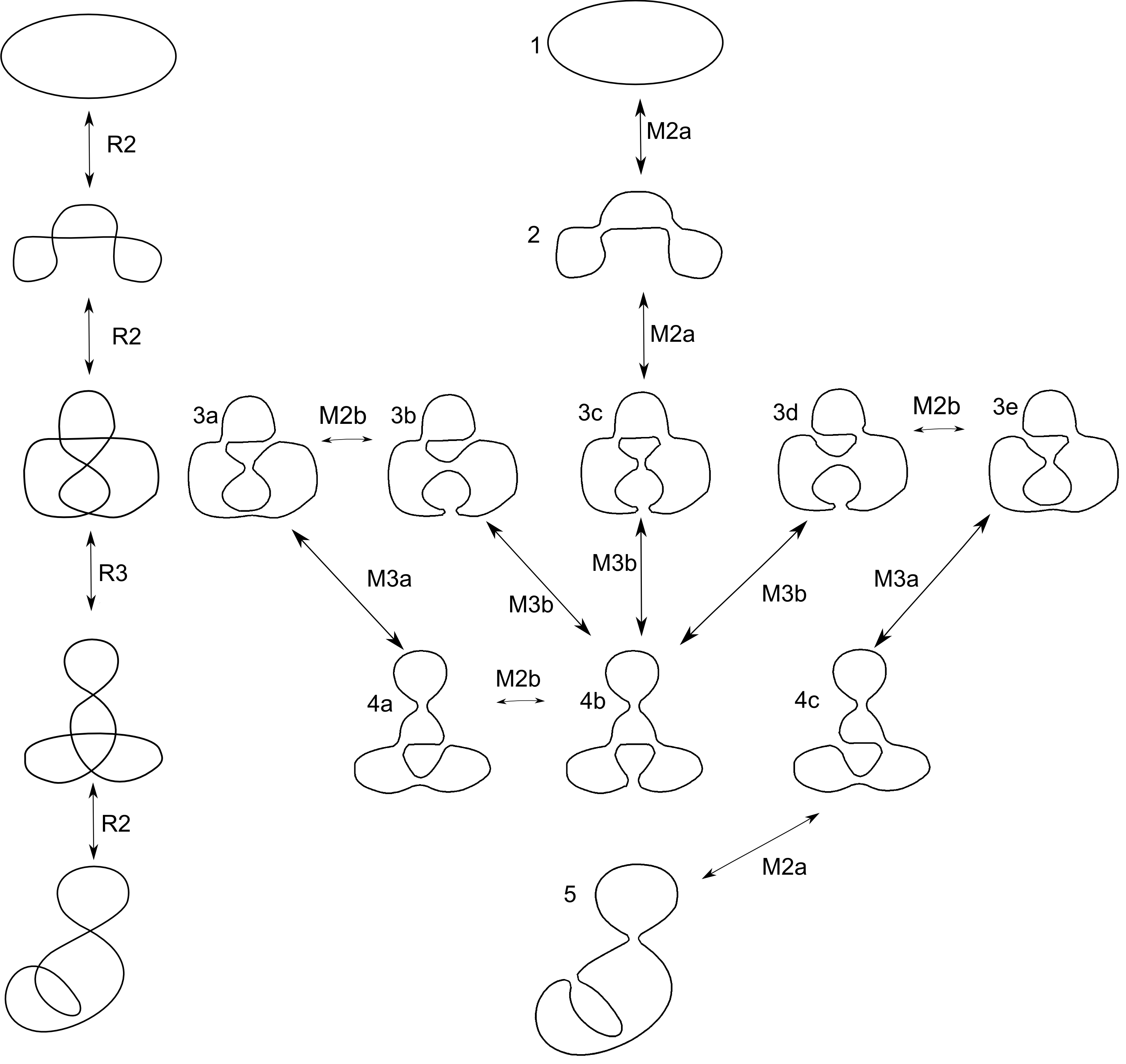
In the left column on Figure 7 there are five curves from a homotopy that starts on a simple closed curve and then goes through Reidemeister moves $R2$, $R2$, $R3$, $-R2$. On the right we consider all possible ways to redraw these curves in such a way so that they are connected and do not have self-intersections. There are 5 different connected redrawings for the third curve and 3 different redrawings for the fourth curve.

We would like to construct an isotopy from the initial simple curve to the redrawing of the last curve. By applying moves $M2a$, $M2a$ and $-M3b$ we obtain an isotopy to the curve $4b$, but then we encounter a problematic $-R2$ move as in Figure 4. By applying move $M2b$ we can homotope $4b$ to $4a$, but then after moves $M3a$, $M2b$, $-M3a$ we get back to $4b$. The solution is to use one of $-M3b$ moves to homotope $4b$ to $3d$, followed by a sequence of moves that homotope it to the curve $5$.

Observe that all curves, except for $1$ and $5$, have an even number of arrows pointing to them. This is a key observation that will be used in the proof below.

We now have to show that this technique is versatile enough to handle any issue that might arise.

We now define a procedure of “resolving” the self-intersections of a curve $\gamma_{t_{j}}$. Let $p$ be a self-intersection point of $\gamma_{t_{j}}$. Consider a small ball $B$ around $p$. If we erase all points in $B$ from $\gamma_{t_{j}}$, we obtain two disconnected curves $\gamma_{t_{j}}\setminus(B\cap\gamma_{t_{j}})$, each with two endpoints. We can reconnect the endpoints in one of the two ways shown in Figure 8, removing the self-intersection $p$. If we execute this procedure for every self-intersection of $\gamma_{t_{j}}$, we either obtain a single simple closed curve which is $\epsilon$-image equivalent to $\gamma_{t_{j}}$, or several disconnected simple closed curves. We only consider sets of reconnections which result in single simple closed curves, and will call such a set a resolution.

We define a sign of a reconnection in a resolution as follows. Fix an orientation of the curve. Consider a small neighbourhood of the intersection and let $a_{1}$ and $a_{2}$ denote two intersecting arcs in this neighbourhood. If we remove a small ball around the intersection point, each $a_{i}$ is cut into two subarcs $a_{i}^{1}$ and $a_{i}^{2}$, where the order of subarcs is defined by the orientation of $\gamma_{t_{j}}$. If the resolution connects $a_{1}^{1}$ to $a_{2}^{2}$ we call it positive, and if it connects $a_{1}^{1}$ to $a_{2}^{1}$ we all it negative. Observe that this definition of sign is independent of the choice of orientation of the curve.

The isotopy we construct will consist of curves that are obtained from the curves of the homotopy by resolving all of their self-intersections in the way just described. By selecting the balls around the intersections to be small enough, we ensure that the resolved curves are $\epsilon$-image equivalent to the original curves.

Let $\{G^{j}_{i}\}$ denote the set of all connected curves that can be obtained from $\gamma_{t_{j}}$ by resolving all of its self-intersections. Construction of the isotopy relies on connectedness properties of a certain finite graph $\Gamma$. For each $G^{j}_{i}$, we add a vertex to $\Gamma$, and label it “$G^{j}_{i}$”. We will now define edges of $\Gamma$. It will follow from how these edges are added to $\Gamma$ that, if vertices with labels $G^{j}_{i}$ and $G^{l}_{k}$ are connected by an edge, then there exists an isotopy between corresponding resolutions of $\gamma_{t_{j}}$ and $\gamma_{t_{l}}$ through curves that are $\epsilon-$image equivalent to some subset of curves in the original homotopy, hence achieving the desired length bound. We will show that there exists a path in this graph from the vertex corresponding to curve $\gamma_{0}$ to a vertex corresponding to a simple closed curve which is $\epsilon$-image equivalent to $\gamma_{1}$. Since this path corresponds to an isotopy, we will be done.

All edges that are added to $\gamma$ are either between $G^{j}_{i}$ and $G^{j+1}_{k}$, for $j<n$, or between $G^{j}_{i}$ and $G^{j}_{k}$ for $i\neq k$. We call the first type of edges vertical edges, and the second type of edges horizontal edges.

Let $R_{j}$ denote the Reidemeister move between times $t_{j}$ and $t_{j+1}$, $j<n$. If $R_{j}=\pm R1$, we connect vertices $G^{j}_{i}$ and $G^{j+1}_{k}$ by an edge if the corresponding curves are related by the move $\pm M1$.

If $R_{j}=R3$, we connect $G^{j}_{i}$ and $G^{j+1}_{k}$ if they are related by $M3a$. If $G^{j}_{i}$ is related to $G^{j+1}_{k_{1}}$ by $M3b$, then there must be two other distinct curves $G^{j+1}_{k_{2}}$ and $G^{j+1}_{k_{3}}$ related to $G^{j}_{i}$ by $M3b$. This defines 3 edges in $\Gamma$. Similarly, if $G^{j+1}_{i}$ is related to $G^{j}_{k_{1}}$ by $-M3b$, then there must be two other curves $G^{j}_{k_{2}}$ and $G^{j}_{k_{3}}$ related to $G^{j}_{i}$ by $-M3b$. This also defines $3$ edges.

If $R_{j}=\pm R2$ we connect two vertices if the corresponding curves are related by a $\pm M2$ move. If $G^{j}_{i}$ has intersections resolved as in Figure 4 and $R_{j}$ removes intersections in a $-R2$ move, then we do not connect $G^{j}_{i}$ to any vertex on the level corresponding to $j+1$. Similarly, for a curve $G^{j+1}_{i}$ that has intersections resolved as in Figure 4 and created by an $R2$ move, we do not connect $G^{j+1}_{i}$ to any vertex on the $j$th level. Instead, we will connect these vertices with a vertex on the same level by a horizontal edge.

Consider a curve $G^{j}_{i}$ with intersections $a$ and $b$ resolved as in Figure 4. We then have that there exists a curve $G^{j}_{k}$, which is identical to $G^{j}_{i}$ except that the corresponding intersections have both been resolved with opposite signs. If the preceding move was an $R2$ creation of $a$ and $b$ we connect $G^{j}_{k}$ and $G^{j}_{i}$ by an edge. Similarly, if the next move is a $-R2$ destruction of $a$ and $b$ we also connect $G^{j}_{k}$ and $G^{j}_{i}$ by an edge. Observe that both of these may happen. In that case, vertices $G^{j}_{i}$ and $G^{j}_{k}$ are connected by 2 edges.

We can now complete the proof of Theorem $1.1^{\prime}$. Observe that, by construction, if $j\not\in\{0,n\}$, then $G^{j}_{i}$ is the endpoint of an even number of edges. More specifically, it will be the endpoint of 2, 4, or 6 edges, depending on the preceding and following Reidemeister moves. Let $\Gamma_{0}$ be the connected component of the graph $\Gamma$ that contains $G^{0}_{0}=\gamma_{0}$. By Euler’s degree sum formula (also known as handshaking lemma), there will be an even number of vertices with odd degree in $\Gamma_{0}$. Hence, there exists a path $p$ in $\Gamma$ from $G^{0}_{0}$ to some $G^{n}_{i}$.

If two vertices of $\Gamma$ are connected by an edge, then clearly there exists a isotopy between the corresponding curves described in Figures 2 and 6. Hence, $p$ defines a homotopy of simple curves from $\gamma_{0}$ to a curve $\epsilon-$image equivalent to $\gamma_{1}$ through simple curves $\epsilon-$image equivalent to curves in the homotopy $\gamma$.

The only item left to prove is that, if $\gamma_{1}$ is simple or is a point, then the isotopy ends at $\gamma_{1}$. If it is simple, then we can perturb our homotopy so that, after it is perturbed, $\gamma_{1}$ is still the endpoint as per Lemma 2.2. The above procedure does not affect $\gamma_{1}$ (up to orientation) and so the isotopy ends at $\pm\gamma_{1}$, where $-\gamma_{1}$ is $\gamma_{1}$ oriented in the opposite direction. If $\gamma_{1}$ is a point $p$, then we can perturb our homotopy so slightly so that the endpoint is a simple closed curve which can be contracted through simple closed curves of length at most $\epsilon$ to $p$. By the above argument, our isotopy then ends at this small curve, which can then be contracted to $p$ through small simple closed curves, as desired. This completes the proof of Theorem $1.1^{\prime}$.

As a corollary we give a short proof of the Jordan-Schoenflies theorem.

Recall that a theorem of Baer and Epstein states that if two closed curves on a 2-surface $M$ are homotopic, but not contractible, then they are isotopic. If the two curves are contractible, then the theorem does not hold when $M$ is any orientable surface except for a sphere. Indeed, for these orientable surfaces, an isotopy preserves orientation, so two null-homotopic curves of opposite orientation are homotopic, but not isotopic.

In this section we use Theorem $1.1^{\prime}$ to prove Theorem 1.1, an effective version of the result of Baer and Epstein.

Remark. Any two simple curves on a 2-sphere are isotopic, however, Theorem 1.1 does not hold for simple curves on $S^{2}$. Indeed, consider $S^{2}$ with the standard metric and orientation, and consider a positively oriented circle $\gamma$ of length $\frac{1}{100}$. There exists a homotopy from $\gamma$ to $-\gamma$ through curves of length $\leq\frac{1}{100}$, but any isotopy between them must go through a curve of length $\geq 2\pi$. We conjecture that, if a simple curve $\gamma$ is homotopic to a curve of opposite orientation through a homotopy of curves of length $<L$, then for any $\epsilon>0$ there exists a contraction of $\gamma$ to a point through curves of length at most $L+\epsilon$. Finally, we conjecture that Theorem 1.1 is true for contractible simple closed curves on a non-orientable surface.

In this section we prove Theorem 1.2, the quantitative version of the fact that orientable surfaces have no elements of order $2$ in their fundamental groups.

Let $M$ be an orientable surface and $\alpha$ a closed curve on $M$. Suppose $\gamma$ is a smooth homotopy with $\gamma_{0}=2\alpha$. Let $\alpha$ be parametrized by $[0,1]$, with $\alpha(0)=\alpha(1)$.

Since $M$ is orientable, we can define a continuous unit normal $n(s)$ to $\alpha(s)$. Let $\alpha_{\epsilon}(s)$ denote the value of the exponential map at $\alpha(s)$ evaluated at $\epsilon n(s)$ for sufficiently small values of $\epsilon$. Let $f$ be a smooth bump function supported (and non-zero) on the open interval $(\frac{1}{2},1)$, and attaining maximum at $f(\frac{3}{4})=1$. We define a homotopy of $2\alpha$ to a curve $\beta$:

We can make a small perturbation to $\alpha$ that increases its length by an arbitrarily small amount, and which removes all non-normal self-intersections (see the proof of Proposition 2.1). The original and perturbed versions of $\alpha$ are clearly homotopic through curves that are larger than $L$ by an arbitrarily small amount. As such, choosing $\epsilon$ to be small enough, $\beta$ also has only normal self-intersections, and its length is only larger than that of $\alpha$ by an arbitrarily small amount. If $\alpha$ has $k$ self-intersections, then $\beta$ has $4k+1$ intersections, as in Figure 10. Since $\beta$ is a small perturbation of $2\alpha$, there exists a small perturbation of $\gamma$ that starts at $\beta$ and satisfies the conclusions of Lemma 2.2. For simplicity we will assume that $\gamma$ has already been put into this form.

To proof the theorem we need to construct a homotopy of $\beta([0,\frac{1}{2}])$ to a point that goes through subcurves of $\gamma$.

The method that we use will be similar to that employed to prove Theorem $1.1^{\prime}$: we will construct a graph $\Gamma$ which contains a path that will be used to define the desired homotopy. As in the proof of this theorem, let

be times at which $\gamma_{t_{i}}$ contains only normal self-intersections, and between which exactly one Reidemeister move occurs. Let $\{p_{i}^{j}\}$ be the set of intersection points of $\gamma_{t_{j}}$, $1\leq i\leq k_{j}$.

As before, we will begin by defining how vertices are added to $\Gamma$. For each $p_{i}^{j}$, add a vertex to $\Gamma$, and label it “$p_{i}^{j}$”. Additionally, for each $j$ with $0\leq j\leq n$, add a vertex to $\Gamma$ with label “$p_{0}^{j}$” (these will correspond to an “empty self-intersection” at each point $t_{j}$).

We will now define the edges of $\Gamma$ as follows. Let $R_{j}$ denote the Reidemeister move between $t_{j}$ and $t_{j+1}$. Again, we will add certain “vertical” edges between vertices with labels $p_{i}^{j}$ and $p_{k}^{j+1}$, followed by certain “horizontal” edges between vertices with labels $p_{i}^{j}$ and $p_{k}^{j}$.

Edges of $\beta$. We now define some additional edges between vertices $p_{i}^{0}$, $i\geq 1$, which correspond to self-intersection points of $\beta$. We will do this with the aid of Figure 12. This figure shows $2$ arcs from $\beta([0,\frac{1}{2}])$ in bold, and the corresponding $2$ arcs from $\beta([\frac{1}{2},1])$ as doted lines. Let $p_{i_{1}}^{0}$, $p_{i_{2}}^{0}$, $p_{i_{3}}^{0}$, and $p_{i_{4}}^{0}$ be as in the figure. $p_{i_{1}}^{0}$ and $p_{i_{2}}^{0}$ correspond to a double intersection of $2\alpha$, moved apart when $2\alpha$ was perturbed into $\beta$, and $p_{i_{3}}^{0}$ and $p_{i_{4}}^{0}$ are created during this perturbation. For each such cluster of $4$ self-intersection points, we add an edge between $p_{i_{1}}^{0}$ and $p_{i_{2}}^{0}$, and we add an edge between $p_{i_{3}}^{0}$ and $p_{i_{4}}^{0}$.

Let $F$ denote the following subset of vertices of $\Gamma$

Observe that by construction, any vertex that is not in $F$ has exactly $2$ edges. Hence, there exists a path $P$ in $\Gamma$ from $p^{0}_{1}$ to a vertex in $F\setminus\{p^{0}_{1}\}$.

We use $P$ to construct a homotopy of $\beta([0,\frac{1}{2}])$ to a subcurve of $\gamma_{1}$ through subcurves of $\gamma$. It may happen that in the process of this homotopy $\beta([0,\frac{1}{2}])$ is contracted to a point.

Note that $\gamma_{t_{j}}^{-1}(p^{j}_{i})$ subdivides $S^{1}$ into two intervals $I_{1}$ and $I_{2}$. Let $(C^{j}_{i})_{1}$ and $(C^{j}_{i})_{2}$ denote the two closed curves $\gamma_{t_{j}}|_{I_{1}}$ and $\gamma_{t_{j}}|_{I_{2}}$. In the case of $p^{j}_{0}$, $(C^{j}_{0})_{\{1,2\}}$ are a point and the entire curve. The next lemma will show us that paths in $\Gamma$ correspond to homotopies through subcurves.

By examining the degrees of the vertices we see that there exists a path from $p^{0}_{1}$ to some other vertex in $F$. Hence, there exists a homotopy of $\beta([0,\frac{1}{2}])$ that either contracts it to a point, or homotopes it to $\gamma_{t}$ for some time $t$ over curves which are longer than $L$ by an arbitrarily small amount. Since $\gamma_{t}$ is also contractible over curves with this same length bound, this completes the proof of Theorem $1.2^{\prime}$. From the remarks in the introduction, we have that Theorem 1.2 is true, too.

Remark. It is natural to ask whether the same result holds for $m$ iterates of a curve. The above proof does not directly generalize to this situation. Consider, for example, a simple closed curve $\alpha$, such that $\beta=3\alpha$ can be contracted to a point through curves of length $\leq L$. A small perturbation of $\beta$ (analogous to $\sigma_{t}$ in the proof above) has two self-intersection points. Each of the self-intersection points divides $\beta$ into two subcurves, one of which is a perturbation of $\alpha$ and the other is a perturbation of $2\alpha$. Denote these subcurves by $A_{1}$ and $A_{2}$ for the first self-intersection point, and $B_{1}$ and $B_{2}$ for the second.

We can consider homotopies of these 4 subcurves and apply the same method of tracking the self-intersection point as in the proof above. For certain homotopies of $\beta$, however, this will produce a homotopy between pairs $A_{1}$ and $B_{1}$, $A_{2}$ and $B_{2}$, giving us no information on how $\alpha$ can be contracted.

The authors have partial results on this problem that will appear in an upcoming article.

In this section we give some higher dimensional counterexamples to Theorems 1.2 and $1.2^{\prime}$.

We remark that Theorems 1.1 and $1.1^{\prime}$ do not hold for curves on a manifold of dimension 3 because of the existence of non-trivial knots. In higher dimensions they trivially hold since curves in a generic homotopy do not have self-intersections.

We begin with a definition:

Theorem 1.2 implies the following:

This is not true in higher dimensions.

References

- [A] V. I. Arnold, Wave front evolution and equivariant Morse lemma, Comm. Pure Appl. Math. 6, 29 (1976), 557 - 582.
- [Ba] R. Baer, Isotopien von Kurven auf orientierbaren, geshlossenen Fächen, Journal für die Reine und Angewandte Mathematik, 159 (1928), 101 - 116.
- [BM] K. Burns, V. Matveev, Open problems and questions about geodesics, preprint math arXiv:1308.5417.
- [Bru] J. W. Bruce, On transversality, Proc. Edinburgh Math. Soc. 29 (1986) 115 - 123.
- [CR] G. R. Chambers, and R. Rotman, Contracting loops on a Riemannian -surface, preprint, math arXiv:1311.2995.
- [D] J.-P. Dufour, Familles de courbes planes différentiables, Topology 4, 22 (1983), 449 - 474.
- [E] D. B. A. Epstein, Curves on 2-manifolds and isotopies, Acta Math. 115 (1966), 83 - 107.
- [GG] M. Golubitsky, and V. Guillemin, Stable mappings and their singularities, Springer-Verlag, 1974.
- [HR] N. Hingston, H.-B. Rademacher, Resonance for loop homology of spheres, J. Differential Geom. Volume 93, Number 1 (2013), 133 - 174.
- [H] M. W. Hirsch, Differential Topology, Springer-Verlag, 1994.
- [K] K. Murasugi, Knot theory and its applications, Birkhäuser, 1996.