Frequency lock closed-loop control of a separated flow using visual feedback

Experiments were carried out in a hydrodynamic channel in which the flow is driven by gravity. The flow is stabilized by divergent and convergent sections separated by honeycombs. The test section is $80$ cm long with a rectangular cross section $15$ cm wide and $10$ cm high.
The quality of the main stream can be quantified in terms of flow uniformity and turbulence intensity. The standard deviation $\sigma$ is computed for the highest free stream velocity featured in our experimental set-up. We obtain $\sigma=0.059$ cm.s^-1 which corresponds to turbulence levels of $\frac{\sigma}{U_{\infty}}=0.0023$.
The mean free stream velocity $U_{\infty}$ can go up to $22$ cm.s^-1 leading to a maximum Reynolds number $Re_{h}=\frac{U_{\infty}h}{\nu}=2800$. A specific leading-edge profile is used to smoothly start the boundary layer which then grows downstream along the flat plate, before reaching the edge of the step $33.5$ cm downstream. The boundary layer is laminar and follows a Blasius profile. More details can be found in Cambonie, Gautier, and Aider [12].

The BFS geometry and the main geometric parameters are shown in figure 1. BFS height is $h=1.5$ cm. Channel height is $H=7$ cm for a channel width $w=15$ cm. The vertical expansion ratio is $A_{y}=\frac{H}{h+H}=0.82$ and the spanwise aspect ratio is $A_{z}=\frac{w}{h+H}=1.76$.

The flow is seeded with 20 $\mu m$ neutrally buoyant polyamid seeding particles. They are illuminated by a laser sheet created by a 2W continuous laser beam operating at $\lambda=532$ nm. Images of the symmetry plane are recorded using a Basler acA 2000-340km 8bit CMOS camera. Velocity field computations are run on a Gforce GTX 580 graphics card.

The algorithm used to compute the velocity fields is a Lukas-Kanade optical flow algorithm [13] called FOLKI developped at ONERA. Its offline and online accuracy have been demonstrated and detailed by Champagnat et al. [14], Gautier and Aider [15]. The algorithm was used off-line by Davoust, Jacquin, and Leclaire [16], Sartor, Losfeld, and Bur [17]. The GPU version (FOLKI-GPU) was improved [15] to allow for the computation of instantaneous velocity fields in real time at a sampling frequency $f_{s}$ up to 100 Hz. Thus the state of the flow can be computed in real-time up to 100 Hz and then be used as an input in closed-loop control. Another advantage of the optical flow algorithm is its ability to compute accurate velocity fields even when velocity changes by as much as a factor of 2 without adjusting acquisition or computation parameters. Fields are $17.2\times 4.6$ cm² and capture the whole recirculation regardless of Reynolds numbers.

Actuation is provided by a flush slot jet, 0.1 cm long and 9 cm wide. Injection is normal to the wall. The distance between the injection slot and step edge is $d=3.5$ cm $=2.3h$ (figure 1). Water coming from a pressurized tank enters a plenum and goes through a volume of glass beads designed to homogenize the incoming flow. Jet amplitude is controlled by changing tank pressure.
The flow is modulated by a one-way voltage driven solenoid-valve. A constant amplitude square signal is sent to the valve. The duty cycle $dc$, defined as the ratio between the time during which the valve is opened $T_{on}$ and total cycle time $T_{ac}$, is kept constant at $dc=\frac{T_{on}}{T_{ac}}=20$ % which has been shown to be an optimal value for this setup [18]. The only varying actuation feature is the frequency of the actuation $F_{ac}$.

The most commonly used variable to quantify the state of the flow downstream the BFS is the length of the recirculation bubble [4, 5, 6]. However, the recirculation area $A_{rec}$ has been shown to be a proper state parameter, easier to compute when using 2D instantaneous velocity fields [7, 15, 18]. Because $A_{rec}$ is computed using the whole 2D flow field, it is able to better capture the influence of actuation on flow structures near the step edge and its influence on the whole recirculation bubble. It is computed over the 2D velocity field:

where A is the 2D velocity field area, H is the Heaviside function and $v_{x}$ the longitudinal velocity.

Kelvin-Helmholtz spanwise vortices created in the shear layer of the BFS (figure 1) strongly influence the recirculation area. Using optical flow instantaneous velocity measurements allows the detection of KH vortices as they are shed in the shear layer. An effective way of detecting vortices is to compute the swirling strength criterion $\lambda_{ci}(s^{-1})$ in the instantaneous two-components velocity fields. This criterion was first introduced and subsequently improved by Chong, Perry, and Cantwell [19], Zhou et al. [20] who analyzed the velocity gradient tensor and proposed that the vortex core be defined as a region where $\nabla\bf{u}$ has complex conjugate eigenvalues. For 2D data $\lambda_{Ci}$ can be computed quickly and efficiently following equation 2:

when such a quantity is real, else $\lambda_{Ci}=0$. The shedding frequency is obtained by spatially averaging $\lambda_{Ci}$ in the vertical direction at $x=5h$. The sampling frequency is $f_{s}=$ 60Hz. This is equivalent to counting vortices as they pass through an imaginary vertical line (Figure 2a). Figure 2b shows a typical time series of fluctuations of $\lambda_{Ci}(t)$ for $Re_{h}=2900$. Every peaks correspond to a vortex moving across the $x=5h$ line. Figure 2c shows the corresponding frequency spectrum obtained by Fourier transform. The natural shedding frequency $f_{KH}$ is well defined. It leads to a Strouhal number based on the step height $St_{h}=\frac{f_{KH}h}{U_{0}}=0.291$ for the KH shedding frequency.

Because recirculation changes with $Re_{h}$ and control actuation it is important to choose a position where shedding frequency can be computed reliably. This is done by placing the detection zone such that initial vortex shedding position is always upstream whatever the operating conditions. In practice this is achieved by placing the detection zone sufficiently downstream the BFS, in this case at $x=5.0h$.

The closed-loop control algorithm is described in figure 3. A new quantity, called $u_{check}(t)$, is introduced. It corresponds to the longitudinal velocity field spatially averaged in the upper corner of the velocity fields, far from the boundaries. When the external flow is stabilized, i.e. when $u_{check}(t)$ does not change for a given period $\Delta T_{steady}$, then the shedding frequency $f_{KH}$ is computed over a given time $\Delta T_{computation}$. Once $f_{KH}$ has been estimated, the control begins: the jet starts pulsing at resulting $f_{ac}=f_{KH}$. At this point shedding frequency is locked to pulse frequency leading, in principle, to a minimization of the recirculation area.
The actuation is kept constant as long as $\Delta u_{check}$ does not change. This is done by continuously polling the value described in equation 3. It is a measure of how much the flow has changed since the last frequency computation. If the value goes above a given threshold, frequency is re-computed, thus completing the loop. The threshold depends on the noise of the monitoring variable and should be chosen such that only significant changes prompt re-computation.

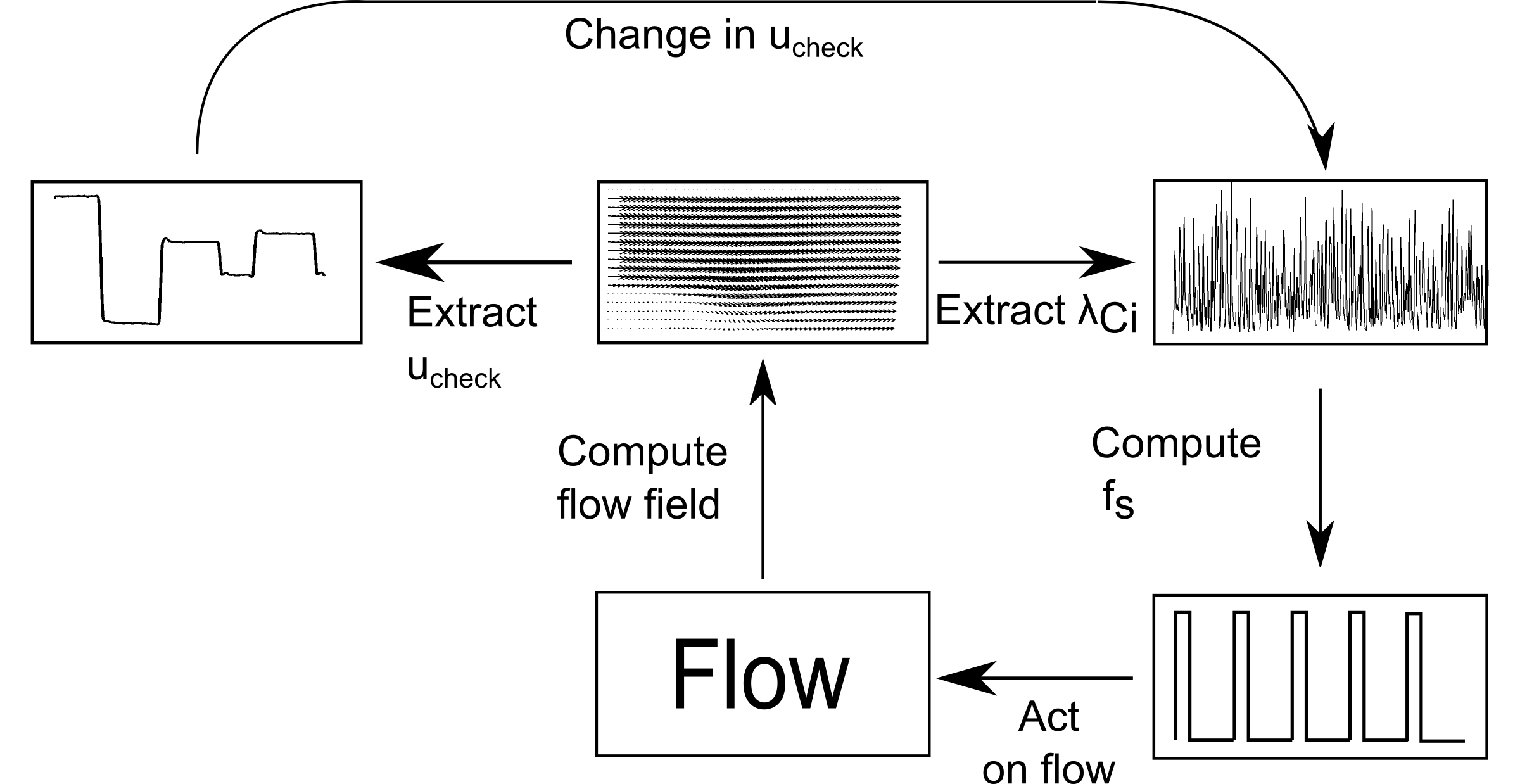
Here $u_{check}$ is chosen to determine whether frequency can be reliably computed but many other quantities might be used as inputs. $\Delta T_{steady}$ should be chosen such that computation starts after there are no significant changes in the monitoring variable. This can be done by taking a value greater than the characteristic time scale of the system. $\Delta T_{computation}$ must be chosen so that $f_{KH}$ can be reliably computed. Small variations in $f_{KH}$ for the same input flow can be allowed since the flow is sensitive to actuation close to $f_{KH}$. Longer checking and computation times ensure a more reliable but less responsive system.

To demonstrate the efficiency of the frequency-lock approach, the free-stream velocity is randomly varied. Variations in $Re_{h}$ (based on $u_{check}$) are shown in figure 4a. To ensure strong variations in the KH frequency, a wide range of Reynolds number is explored ($Re_{h}=1400$ to $2800$). Each time the Reynolds number is changed, the KH frequency is evaluated, as shown on figure 4b.

Finally, figure 4c shows the evolution of $A_{rec}(t)$ normalized by $h^{2}$ as a function of time. The mean value is also computed over each controlled phase (red lines on figure 4c). Re-computation only occurs for major changes in $u_{check}$. What constitutes major changes is up to the user. Because shedding frequency is locked during control to actuation frequency, control is successful even when natural shedding frequency varies slightly. Every large peaks in $A_{rec}(t)$ correspond to a re-computation of $f_{KH}$. As a consequence, each peak corresponds to the uncontrolled value associated to the new value of the Reynolds number. When the flow is controlled, reduction in $A_{rec}$ varies between 70 % to 85 % when compared to the uncontrolled value. These values are consistent with those found by Gautier and Aider [18] in open-loop experiments. It clearly demonstrates the robustness of this control strategy based on frequency lock on a natural frequency estimated by real-time instantaneous optical measurements.

References

- [1] B. F. Armaly, F. Durst, J. C. F. Pereira, and B. Schonung, “Experimental and theoretical investigation of backward-facing step flow,” Journal of Fluid Mechanics 127, 473–496 (1983).
- [2] V. Uruba, P. Jonas, and O. Mazur, “Control of a channel-flow behind a backward-facing step by suction/blowing,” Heat and Fluid Flow 28, 665–672 (2007).
- [3] J.-L. Aider, A. Danet, and M. Lesieur, “Large-eddy simulation applied to study the influence of upstream conditions on the time-dependant and averaged characteristics of a backward-facing step flow,” Journal of Turbulence 8 (2007).
- [4] K. B. Chun and H. J. Sung, “Control of turbulent separated flow over a backward-facing step by local forcing,” Experiments in Fluids 21, 417–426 (1996).
- [5] R. Becker, M. Garwon, C. Gutknecht, G. Barwolff, and R. King, “Robust control of separated shear flows in simulation and experiment,” Journal of Process Control 15, 691–700 (2005).
- [6] L. Henning and R. King, “Robust multivariable closed-loop control of a turbulent backward-facing step flow,” Journal of Aircraft 44 (2007).
- [7] N. Gautier and J.-L. Aider, “Control of the flow behind a backwards facing step with visual feedback,” Royal Society Proceedings A 469 (2013a).
- [8] T. Duriez, J.-L. Aider, and J. E. Wesfreid, “Self-sustaining process through streak generation in a flat-plate boundary layer,” Physical review letters 103, 144502 (2009).
- [9] P. Joseph, X. Amandolese, C. Edouard, and J.-L. Aider, “Flow control using mems pulsed micro-jets on the ahmed body,” Experiments in Fluids 54, 1–12 (2013).
- [10] J.-F. Beaudoin, O. Cadot, J.-L. Aider, and J.-E. Wesfreid, “Drag reduction of a bluff body using adaptive control methods,” Physics of Fluids 18, 085107 (2006).
- [11] M. Pastoor, R. King, B. R. Noack, A. Dillmann, and G. Tadmor, “Model-based coherent-structure control of turbulent shear flows using low-dimensional vortex models,” American Institute of Aeronautics and Astronautics na, na (2003).
- [12] T. Cambonie, N. Gautier, and J.-L. Aider, “Experimental study of counter-rotating vortex pair trajectories induced by a round jet in cross-flow at low velocity ratios,” Experiments in Fluids 54, 1–13 (2013).
- [13] G. L. Besnerais and F. Champagnat, “Dense optical flow by iterative local window registration,” in ICIP (1) (2005) pp. 137–140.
- [14] F. Champagnat, A. Plyer, G. Le Besnerais, B. Leclaire, S. Davoust, and Y. Le Sant, “Fast and accurate piv computation using highly parallel iterative correlation maximization,” Experiments in Fluids 50, 1169–1182 (2011).
- [15] N. Gautier and J.-L. Aider, “Real time, high frequency planar flow velocity measurements,” Submitted Journal of Visualization, avalaible at arXiv under Real-time planar flow velocity measurements using an optical flow algorithm implemented on GPU (2013b).
- [16] S. Davoust, L. Jacquin, and B. Leclaire, “Dynamics of m = 0 and m = 1 modes and of streamwise vortices in a turbulent axisymmetric mixing layer,” Journal of Fluid Mechanics 709, 408–444 (2012).
- [17] F. Sartor, G. Losfeld, and R. Bur, “Piv study on a shock-induced transition in subsonic flow,” Experiments in Fluids 53, 815–827 (2012).
- [18] N. Gautier and J.-L. Aider, “Effects of pulsed actuation upstream a backward-facing step,” Proceedings GDR2502 Controle Des Decollements .
- [19] M. Chong, A. Perry, and B. Cantwell, “A general classification of 3-dimensional flow fields,” Physics of Fluids 2, 765–777 (1990).
- [20] J. Zhou, R. Adrian, S. Balachandar, and T. Kendall, “Mechanisms for generating coherent packets of hairpin vortices,” J Fluid Mech 387, 535–396 (1999).