Particle filter-based Gaussian process optimisation for parameter inference
Abstract
We propose a novel method for maximum likelihood-based parameter inference in nonlinear and/or non-Gaussian state space models. The method is an iterative procedure with three steps. At each iteration a particle filter is used to estimate the value of the log-likelihood function at the current parameter iterate. Using these log-likelihood estimates, a surrogate objective function is created by utilizing a Gaussian process model. Finally, we use a heuristic procedure to obtain a revised parameter iterate, providing an automatic trade-off between exploration and exploitation of the surrogate model. The method is profiled on two state space models with good performance both considering accuracy and computational cost.
1 Introduction
We are interested in maximum likelihood-based (ML) parameter inference in nonlinear and/or non-Gaussian state space models (SSM). An SSM with latent states and measurements is defined as
| (1a) | ||||
| (1b) | ||||
where and denote known distributions parame- trised by the unknown static parameter vector . For simplicity, we assume that the initial state is known. Let denote the likelihood of for a given value of . In ML estimation, we wish to estimate by solving the optimisation problem,
| (2) |
where denotes the log-likelihood function. Extensive treatments on ML inference are found in e.g. [18] and [14].
The likelihood for a general SSM can be expressed as
| (3) |
where denotes the one-step predictive density. For a linear Gaussian models, these densities can be computed exactly by using the Kalman filter. However, for a nonlinear model the one-step predictive densities are in general intractable. It is therefore also intractable to evaluate the objective function in (2), which poses an obvious difficulty in addressing the ML problem.
Recently, ML estimation has been carried out in nonlinear SSMs by the aid of Sequential Monte Carlo [7]. This includes e.g. using gradient-based search [22] and the Expectation Maximisation (EM) algorithm [24, 16]. However, some of these methods require computationally costly particle smoothing to estimate the necessary quantities, which can be a problem in some situations.
An alternative is to make use of the simultaneous perturbation stochastic approximation (SPSA) algorithm [26], which uses a steepest ascent algorithm with a stochastic approximation scheme to estimate the solution to (2). The gradients are estimated using finite differences with random perturbations. This results in that the algorithm only needs to sample the likelihood function twice at each iteration, independent of the dimension of the problem. SPSA is used in combination with SMC in e.g. [25] and [9].
Another approach for maximum likelihood estimation is based on approximate inference based on Laplace approximations and moment matching. We do not consider these methods any further in this paper and refer interested readers to e.g. [2], [13] and [1] for more information.
In this paper, we propose a novel algorithm for ML estimation of static parameters in a nonlinear SSM. The method combines particle filtering (PF) with Gaussian process optimisation (GPO) [11, 3, 17]. The latter is a method well-suited for optimisation when it is costly to evaluate the objective function. The resulting algorithm is efficient in the sense that it provides accurate parameter estimates while making use of only a small number of (costly) log-likelihood evaluations.
2 Maximum likelihood estimation with a surrogate cost function
We now turn to our new procedure for ML estimation of general nonlinear SSMs (1). We start by outlining the main ideas of the procedure on a high level. The individual steps of the algorithm are discussed in detail in the consecutive sections. The algorithm is an iterative procedure, which thus generates a sequence of iterates for the model parameters. Each iteration consists of three main steps:
- (i)
Given the current iterate , compute an estimate of the objective function (i.e. the log-likelihood) for this parameter value, denoted as .
- (ii)
Given the collection of tuples generated up to the current iterate, create a model of the (intractable) objective function .
- (iii)
Use the model as a surrogate for the objective function to generate a new iterate .
Note that the method requires only one estimation of the log-likelihood function at each iteration. This is promising, since it is typically computationally costly to estimate the log-likelihood value and we therefore wish to keep the number of such evaluations as low as possible.
For step (i), i.e. evaluating the log-likelihood function for a given value of , we use a PF, resulting in a (noisy) estimate of the objective function. This step is discussed in Section 3. For steps (ii) and (iii), we apply the GPO framework. First, we construct a surrogate for the objective function by modelling it as a Gaussian process, taking the information available in the previous iterates into account. This is discussed in Section 4.
Then, we make use of a heuristic, referred to as an acquisition rule, to find the next iterate based on the GP model. The acquisition rule is such that it favours values of for which the model predicts a large value of the objective function and/or where there is a high uncertainty in the model. This is useful since it automatically results in a trade-off between exploration and exploitation of the model.
In this paper, we consider a simple numerical example to illustrate the different steps of the algorithm during the derivation. For this, the linear Gaussian state space (LGSS) model,
| (4a) | ||||
| (4b) | ||||
with and parameter is simulated for time steps. The complete algorithm is evaluated in Section 6 on this model, as well as on a nonlinear SSM.
3 Estimating the log-likelihood
We begin this section with a brief description of a PF. For more general introductions, see e.g. [7]. We then continue with discussing the specific problem of likelihood estimation using the PF.
3.1 The particle filter
The PF is a sequential Monte Carlo method used to approximate e.g. the intractable filtering distribution for a general SSM (1). This is done by representing it by a set of weighted particles according to
where and denote the (unnormalised) weight and state of particle at time , respectively. Here, denotes the Dirac measure located at the point . These approximations are generated sequentially in time . Given the particles at time , the PF proceeds to time by: (a) resampling, (b) propagation and (c) weighting.
In step (a), the particles are resampled with replacement, using the probabilities given by their (normalized) importance weights. This is done to rejuvenate the particle system and to put emphasis on the most probable particles. The result is an unweighted particle system , targeting the same distribution .
In step (b), the particles are propagated to time by sampling from a proposal kernel from to . Finally in Step (c), the particles are assigned importance weights. This is done to account for the discrepancy between the proposal and the target densities. The importance weights are given by
| (5) |
In the sequel, we use the bootstrap PF which means that new particles are proposed according to the state dynamics, i.e. and . Although more sophisticated alternatives exist, see e.g. the fully-adapted PF introduced in [20].
3.2 Estimation of the likelihood
In order to use the PF for estimating the likelihood, we start by writing the one-step predictive density as
where we have multiplied and divided with the proposal kernel . To approximate the integral, we note that the (unweighted) particle pairs are approximately drawn from . Consequently, we obtain the Monte Carlo approximation
By inserting this approximation into (3) we obtain the particle estimate of the likelihood,
This likelihood estimator has been studied extensively in the SMC literature. The estimator is consistent and, in fact, also unbiased for any ; see e.g. [21] and Proposition 7.4.1 in [6]. Furthermore, a central limit theorem holds,
for some asymptotic variance ; see Proposition 9.4.1 in [6].
3.3 Estimation of the log-likelihood
However, working directly with the likelihood typically results in numerical difficulties. To avoid problems with numerical precision, we instead use an estimate of the log-likelihood
| (6) |
The resulting complete algorithm for estimating the log-likelihood using a PF is presented in Algorithm 1.
Note that, by taking the logarithm of , we introduce a bias into the estimator. However, by the second-order delta method [5], the asymptotic normality carries over to the log-likelihood estimate,
| (7) |
where . Motivated by this, we make the assumption that the log-likelihood estimates are Gaussian distributed and centered around the true log-likelihood value. That is, we can write
| (8) |
Similar normality assumptions have previously been used by [21] and [8]. The unknown variance is treated as a free parameter that is estimated on-the-fly as we run the proposed estimation algorithm. That is, we do not have to estimate by making any initial test runs. We return to this in the sequel.
We validate the Gaussian assumption (8) using a small numerical experiment to illustrate the bias and variance, at a finite number of particles. We calculate estimates of the log-likelihood for the model in (4). This is done by running Algorithm 1 independently times with particles.
In Figure 1, we present the distribution of the error in the estimates together with a QQ-plot. Both plots validate that the estimates are approximatively distributed according to a Gaussian distribution. Also a Lilliefors hypothesis test [15] does not reject the null hypothesis, that the measurements are drawn from a Gaussian distribution at significance level .
4 Modelling the surrogate function
From the previous, we consider a naive approach to solve (2) by creating a grid of the parameter space and estimating the log-likelihood in each grid point. The parameter estimate is then obtained as the grid point that maximises the objective function. The problem here is that as the dimension of the parameter space increases, an exponentially increasing number of grid points is required to retain the accuracy of the estimate.
Furthermore, using finite differences to compute the gradient of the log-likelihood is problematic due to the noise in (8). This problem can be mitigated by using a particle smoother, as previously discussed in e.g. [22], but this is even more computationally expensive than running the particle filter. Instead, we construct a model of the noisy log-likelihood evaluations in Step (ii). This model then serves as a surrogate for the actual objective function.
4.1 Gaussian process model
In this paper, we use a GP for this purpose, as these processes are possibly flexible enough to capture the overall structure of the log-likelihood for many SSMs. GPs can be seen as a generalisation of the multivariate Gaussian distribution and are commonly used as priors over functions. In this view, the resulting posterior obtained by conditioning upon some observations, describes the functions that could have generated the observations. This makes GPs a popular class of nonparameteric models used for e.g. regression, classification and optimisation, see e.g. [23] and [19].
In the following, we model the log-likelihood as being a priori distributed according to a GP. That is,
| (9) |
where the process is fully described by the mean function and the covariance function .
4.2 Updating the model and the hyperparameters
To ease the presentation, we here consider a particular iteration of the GP and the PF. Let denote a set of iterates, where and denote vectors obtained by stacking the parameters and noisy log-likelihood estimates, respectively.
It follows that the posterior distribution is given by
| (10) |
where and denote the posterior mean and variance given the iterates , respectively. By standard results for the Gaussian distribution, we have
| (11a) | ||||
| (11b) | ||||
with , and where denotes a -identity matrix. Here we note that the posterior distribution can be sequentially updated to save computations, see the aforementioned references for details.
In the GP model presented, we use some mean function and covariance function that possibly depend on some unknown hyperparameters. Also, we need to estimate the unknown noise variance in (8). For this, we adopt the emperical Bayes (EB) procedure to estimate these quantities. This is done by numerically optimising the marginal likelihood of the data with respect to the hyperparameters.
4.3 Example of log-likelihood modelling
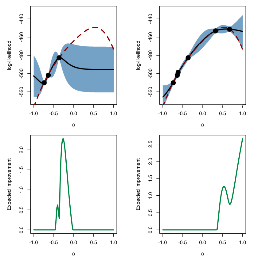
We end this section by an example to illustrate the usefulness of GPs in modelling the log-likelihood. In the upper part of Figure 2, we show the posterior distribution of the log-likelihood of the model in (4). The posterior is estimated using three (left) and six (right) samples of the log-likelihood drawn at some randomly selected parameters. With information from only six samples, the mean of the surrogate function passes close to the observed iterates with a reasonable confidence interval.
5 Acquisition rules
The remaining problem in the proposed algorithm is how to select the parameters at which the log-likelihood should be evaluated in step (iii). A simple choice would be to consider a random sampling approach, which works well when the dimension of the parameters is small. However, when the dimension increases, we are faced with the curse-of-dimensionality and independent sampling is inefficient.
As previously discussed, we instead use acquisition rules that balances exploration and exploitation of the parameter space and makes use of the posterior distribution obtained from the GP. These heuristics are well-studied in GPO and simulation-based comparisons are presented in e.g. [17]. In this paper, we follow their general recommendations and use the expected improvement (EI) from [11].
5.1 Expected improvement
Consider the predicted improvement defined as
| (12) |
where is a user-defined coefficient that balances exploration and exploitation. Also, introduce the expected peak of the log-likelihood function,
| (13a) | ||||
over the previous iterates. Here, we again consider a particular iteration in the notation for brevity.
Finally, by using the posterior distribution obtained from the GP, we can write the EI as
| (14) | ||||
where we drop the dependence on for brevity. Here, and denote the CDF and PDF of the standard Gaussian distribution, respectively. An acquisition rule follows by the maximising argument
| (15) |
i.e. we sample the likelihood in during the next iteration of the algorithm.
In the lower part of Figure 2, the expected improvements are shown for the situation discussed in the previous example. The two situations correspond to an exploitation step (left) and an exploration step (right), respectively. In the former, we sample in the neighbourhood of the current predicted peak. In the latter, we sample in an area where the uncertainty is large to determine if there is a peak in that area.
From the expression in (14), we expect a high value of EI for parameters where the variance is large. If also the predictive mean is larger than , then the EI assumes even larger values for these parameters. This gives the desired behaviour of the acquisition function discussed previously.
Inputs: Algorithm 1, (no. iterations) and (initial parameter).
Output: (est. of the parameter).
6 Numerical illustrations
Finally, we are ready to combine the methods discussed in the previous three sections into the final algorithm and it is presented in Algorithm 2. In the following, we use an LGSS model and a nonlinear model to illustrate the behaviour and the performance of the proposed algorithm. We compare the proposed method in the latter model with the SPSA algorithm [26]. This algorithm is selected as it also only makes use of zero-order information (the log-likelihood estimates) and is known to perform well in many problems, see e.g. [27].
6.1 Implementation details
For the GP, we use a constant mean function and the Matérn kernel with . Note that, other choices of mean functions and kernels (especially the combination of kernels) can possibly improve the performance of the algorithm. This is especially important in models where the log-likelihood in non-isotropic.
The GPML toolbox [23] is used for estimation of the hyperparameters by EB and for the computation of the predictive distribution in (10). For the acquisition function, we use the EI with following the recommendations in [17].
The optimisation in (15) is non-convex and therefore difficult to carry out in a global setting. Two common approaches in GPO are to use multiple local search algorithms in a Monte Carlo setting [17] or using a global optimisation algorithm [4]. In this paper, we use the latter method with the gradient-free DIRECT global optimisation algorithm [12] and the implementation written by Daniel E. Finkel, available from http://www4.ncsu.edu/~ctk/Finkel_Direct/. A maximum of iterations and (cheap) evaluations of the surrogate function are used in the DIRECT algorithm for each optimisation.
6.2 Linear Gaussian state space model
We begin with the LGSS model using one parameter in (4), as this enables us to investigate the behaviour of the proposed algorithm in detail. We use particles, iterations and the initial parameter . In Figure 3, we present the surrogate function and the expected improvement at different iterations. The algorithm converges rather quickly for this simple toy example with the parameter estimate . As a comparison, the MLE obtained by the Kalman filter by maximisation on a grid of parameter values is .

6.3 Nonlinear stochastic volatility model
Consider the Hull-White stochastic volatility model [10],
| (16a) | ||||
| (16b) | ||||
where the parameters are . We use , time steps, particles, iterations and the initial parameter . We implement the SPSA algorithm as suggested by [27] using the recommended settings for the parameters , and . We manually tune the parameters and to achieve good performance for our problem.
The GPO algorithm again converges rather quickly after about evaluations of the log-likelihood and returns the parameter estimate . The SPSA algorithm converges slower and requires more than evaluations of the log-likelihood to reach the neighbourhood of the true parameters. Even more iterations are required for the estimates to stabilise. This shows, for this particular example, that the GPO algorithm could be a competitive choice for maximum likelihood estimation.
7 Conclusions
The results in the previous section indicate that the proposed method does not require many estimates of the intractable log-likelihood. This is due to the GP model that captures the overall structure well and enables an efficient sampling mechanism in the form of the acquisition rule. With this and the comparison with SPSA in mind, we hope that this algorithm shall turn out to be a competitive alternative to more advanced algorithms.
Important future work includes benchmarking of the proposed method, alternative acquisition rules and investigating possibilities for bias-compensation of the log-likelihood estimate. Also, the Gaussian process models can be useful as an alternative to compute the gradient (score function) and negative Hessian (the observed information matrix) of the log-likelihood. Estimating the latter is an important problem in e.g. nonlinear input design, and this approach could decrease the variance in such estimates.
At http://users.isy.liu.se/en/rt/johda87/, we provide source code to reproduce some of the numerical illustrations in this paper.
Acknowledgements
The authors would like to thank Prof. Thomas B. Schön, Dr. Carl E. Rasmussen, Roger Frigola and Andrew McHutchon for interesting discussions and suggestions that greatly improved this paper.
References
- [1] B. M. Bell. The marginal likelihood for parameters in a discrete Gauss-Markov process. IEEE Transactions on Signal Processing, 48(3):870–873, 2000.
- [2] C. M. Bishop. Pattern Recognition and Machine Learning. Springer, New York, USA, 2006.
- [3] P. Boyle. Gaussian processes for regression and optimisation. PhD thesis, 2007.
- [4] E. Brochu, V. M. Cora, and N. De Freitas. A tutorial on Bayesian optimization of expensive cost functions, with application to active user modeling and hierarchical reinforcement learning. Pre-print, 2010. arXiv:1012.2599v1.
- [5] G. Casella and R. L. Berger. Statistical Inference. Duxbury Press, 2 edition, 2001.
- [6] P. Del Moral. Feynman-Kac Formulae - Genealogical and Interacting Particle Systems with Applications. Probability and its Applications. Springer, 2004.
- [7] A. Doucet and A. Johansen. A tutorial on particle filtering and smoothing: Fifteen years later. In D. Crisan and B. Rozovsky, editors, The Oxford Handbook of Nonlinear Filtering. Oxford University Press, 2011.
- [8] A. Doucet, M. K. Pitt, and R. Kohn. Efficient implementation of Markov chain Monte Carlo when using an unbiased likelihood estimator. arXiv.org, arXiv:1210.1871, October 2012.
- [9] E. Ehrlich, A. Jasra, and N. Kantas. Static Parameter Estimation for ABC Approximations of Hidden Markov Models. Pre-print, 2012. arXiv:1210.4683v1.
- [10] J. Hull and A. White. The pricing of options on assets with stochastic volatilities. The Journal of Finance, 42(2):281–300, 1987.
- [11] D. R. Jones. A taxonomy of global optimization methods based on response surfaces. Journal of Global Optimization, 21(4):345–383, 2001.
- [12] D. R. Jones, C. D. Perttunen, and B. E. Stuckman. Lipschitzian optimization without the Lipschitz constant. Journal of Optimization Theory and Applications, 79(1):157–181, 1993.
- [13] M. E. Khan, S. Mohamed, and K. P. Murphy. Fast bayesian inference for non-conjugate gaussian process regression. In Proceedings of the 2012 Conference on Neural Information Processing Systems (NIPS), pages 3149–3157, Lake Tahoe, Nevada, USA, December 2012.
- [14] E. L. Lehmann and G. Casella. Theory of point estimation. Springer, 1998.
- [15] H. W. Lilliefors. On the Kolmogorov-Smirnov Test for Normality with Mean and Variance Unknown. Journal of the American Statistical Association, 62(318):399–402, 1967.
- [16] F. Lindsten. An efficient stochastic approximation EM algorithm using conditional particle filters. In Proceedings of the 38th International Conference on Acoustics, Speech, and Signal Processing (ICASSP), Vancouver, Canada, May 2013.
- [17] D. J. Lizotte. Practical Bayesian optimization. PhD thesis, 2008.
- [18] L. Ljung. System identification: theory for the user. Prentice Hall, 1999.
- [19] K. P. Murphy. Machine learning: a probabilistic perspective. The MIT Press, 2012.
- [20] M. K. Pitt and N. Shephard. Filtering via simulation: Auxiliary particle filters. Journal of the American Statistical Association, 94(446):590–599, 1999.
- [21] M. K. Pitt, R. S. Silva, P. Giordani, and R. Kohn. On some properties of Markov chain Monte Carlo simulation methods based on the particle filter. Journal of Econometrics, 171(2):134–151, 2012.
- [22] G. Poyiadjis, A. Doucet, and S. S. Singh. Particle approximations of the score and observed information matrix in state space models with application to parameter estimation. Biometrika, 98(1):65–80, 2011.
- [23] C. E. Rasmussen and C. K. I. Williams. Gaussian Processes for Machine Learning. MIT Press, 2006.
- [24] T. B. Schön, A. Wills, and B. Ninness. System identification of nonlinear state-space models. Automatica, 47(1):39–49, 2011.
- [25] S. S. Singh, N. Whiteley, and S. J. Godsill. Approximate likelihood estimation of static parameters in multi-target models. In D. Barber, A. T. Cemgil, and S. Chiappa, editors, Inference and Learning in Dynamic Models, pages 225–244. Cambridge University Press, 2011.
- [26] J. C. Spall. A stochastic approximation technique for generating maximum likelihood parameter estimates. In American Control Conference, pages 1161–1167, Minneapolis, MN, USA, June 1987.
- [27] J. C. Spall. Implementation of the simultaneous perturbation algorithm for stochastic optimization. IEEE Transactions on Aerospace and Electronic Systems, 34(3):817–823, 1998.