Classification of two-dimensional Topological Crystalline Superconductors and Majorana Bound States at Disclinations
Abstract
We classify discrete-rotation symmetric topological crystalline superconductors (TCS) in two dimensions and provide the criteria for a zero energy Majorana bound state (MBS) to be present at composite defects made from magnetic flux, dislocations, and disclinations. In addition to the Chern number that encodes chirality, discrete rotation symmetry further divides TCS into distinct stable topological classes according to the rotation eigenspectrum of Bogoliubov-de Gennes quasi-particles. Conical crystalline defects are shown to be able to accommodate robust MBS when a certain combination of these bulk topological invariants is non-trivial as dictated by the index theorems proved within. The number parity of MBS is counted by a -valued index that solely depends on the disclination and the topological class of the TCS. We also discuss the implications for corner-bound Majorana modes on the boundary of topological crystalline superconductors.
I Introduction
The discovery of symmetry protected topological insulators and superconductors has been one of the most exciting developments in condensed matter physics in the last ten years [1, 2]. The most notable symmetry protection is due to time-reversal symmetry [3], but by now the list of possible symmetry protected topological states has vastly expanded. In fact, the closing remarks of Ref. 4 called for a complete topological band theory that includes topological classifications based on all point-group symmetries in addition to the discrete symmetries of time-reversal, charge-conjugation, and chirality. This challenge has been met through the work of several different groups which have begun classifying topological states protected by inversion [5, 6], reflection [4, 7, 8, 9], rotation [10, 11, 12, 13], and in general even more complicated space-group symmetries [14]. In this work we extend the classification to cover all topological crystalline superconductors (TCS) in 2D with discrete rotation symmetries.
In addition to symmetry protected topological insulators and superconductors, the realization of Majorana fermion bound states [15] has become one of the most exciting challenges in the condensed matter community [16, 1, 2, 17, 18] due to its non-Abelian fusion and braiding characteristics [19, 20] and promising prospects in topological quantum computing [21, 22, 23, 24, 25, 26]. These bound states are expected to be present in one and two-dimensional -wave superconductors [27, 28, 29] and in two-dimensional noncentrosymmetric superconductors [30] as boundary or vortex excitations, and in non-Abelian Quantum Hall states [31, 32, 33] as Ising quasi-particle excitations. More recently, with the discovery of topological insulators (TI) [3, 34, 35, 36, 37, 38, 39, 40], Majorana bound states (MBS) are predicted to exist in heterostructures such as superconductor (SC) - ferromagnet (FM) interfaces in proximity with quantum spin Hall insulators [41, 42, 43, 44, 45] and strong spin-orbit coupled semiconductors [46, 47, 48, 49, 50]. They are also predicted to exist in -wave superfluids of cold fermionic atoms with laser-field-generated effective spin-orbit interactions [51].
For the latter cases of heterostructures devices, the MBS are trapped on non-dynamical defects such as domain walls. These defect MBS are conceptually distinct from quantum deconfined Ising anyons in topological phases [52, 53, 54] like the Pfaffian Quantum Hall state [31, 32, 33], the chiral superconductor [28, 29, 19], or the Kitaev honeycomb model [20]. The difference is that they are not fundamental excitations that rely on the existence of non-Abelian topological order of a quantum system, but are extrinsic semiclassical objects associated to a point defect involving a topological winding of a set of order parameters [55, 56]. For example, the existence of MBS at TI-SC-FM heterostructures is a consequence of a topological order parameter texture formed from configurations of the band inversion TI gap, the proximity-induced pairing gap, and the gap due to magnetic order. To prevent the MBS from escaping, the proximity interfaces in a heterostructure are required to be continuous, which may not be easy to achieve in reality. In this paper, we explore the possibility of manifesting defect MBS in a homogeneous time reversal breaking superconductor that does not require strong spin-orbit coupling or extrinsic magnetic fluxes or magnetic moments.
Defects like a quantum vortex in a chiral superconductor [57, 28, 29, 19] or a dislocation when discrete translation symmetry is present in a weak topological phase [58, 56, 59, 60, 61, 13] can bind MBS when a Bogoliubov-de Gennes (BdG) quasi-particle encircling the defect picks up a Berry phase. A single defect MBS in the BdG description has exactly zero energy pinned by particle-hole (or charge conjugation) symmetry. Its existence (or in general the MBS number parity) was shown in Ref. 56 to be topologically determined by a Chern-Simons -invariant [56]
| (1) |
modulo 2, where is the Berry connection of occupied BdG states with momentum in the Brillouin zone (BZ) and at position along a real-space circle around the defect. The index in Eq. 1 captures the interplay between the topology of the bulk BdG Hamiltonian and the structure of the classical defect. For example, the number parities of MBS at a quantum vortex and a dislocation are respectively given by
| (2) |
modulo 2, where is the Chern number that corresponds to the edge chirality of the SC, and the weak invariant characterizes a 2D topological array of weakly coupled SC wires. These quantities are bulk topological information, while the number of flux quanta and dislocation Burgers’ vector are classical defect quantities. We see that the index depends on both, i.e., topological information about the electronic structure and the defect itself.
While the topological index in Eq. 1 completely characterizes the number parity of MBS at any arbitrary point defect in two-dimensional SC, it is not easily applicable to a real material as it requires a continuous diagonalization of a spatially modulated, and sometimes complicated, Hamiltonian. The main objective of this paper is to generalize Eq. 2 into a topological index that applies to a more general class of crystalline defects and only involves detail independent quantities that are in principle experimentally measurable. The special case for disclinations in symmetric TCS, including all layered perovskite structures, was discussed in Ref.13. Here we extend the theorem to all discrete rotation symmetric SC systems. The index that counts MBS number parity takes the following general form:
| (3) |
modulo 2, where are discrete translation and rotation holonomical quantities of a lattice disclination that can be determined experimentally, for example, by neutron scattering, the Chern number and weak invariant correspond to protected gapless edge modes which in theory carry a signature detectable by ARPES or transport, and the rotation invariants are combinations of the rotation eigenvalues of the BdG quasi-particles.
I.1 Outline
Section II begins with a brief review of the classification of two-dimensional BCS superconductors in the BdG framework. The notion of equivariant stable classification is introduced, and is followed by the definitions of integral rotation invariants in a TCS using rotation eigen-spectra at fixed points in the Brillouin zone. The constraints these invariants impose on the Chern and weak invariants is also discussed. Appendices A and B complement this section by providing detailed derivations. Section III, along with Appendix C, proves that the Chern number and rotation invariants completely classify the topology of discrete-rotation symmetric TCS. This section also describes the algebraic structure of the classification, which reveals that a set of primitive models, or generators, can always be constructed to serve as fundamental building blocks of the different topological classes because any arbitrary Hamiltonian is stably topologically equivalent to certain copies of them. Explicit sets of such primitive generator Hamiltonians are constructed for each symmetry, and their classification is shown. These primitive models are either chiral superconductors or rotation symmetric arrays of two-dimensional -wave wires.
Section IV provides a review of the classification of lattice disclinations in terms of their holonomies. Disclination holonomies are composed of a rotation and a translation piece, both of which enter the index theorems for the parity of MBS in and symmetric TCS, while only the rotation part enters the index for and symmetric TCS.
Section V begins by stating the general form of the topological index as a bilinear function of the disclination holonomical quantities (Frank angle and the effective Burgers’ vector) and topological Chern and rotation invariants. The index determines the parity of the number of MBS at a dislocation-disclination-flux composite of an arbitrary TCS described by a BdG Hamiltonian. By numerical and analytical exact diagonalization of the primitive model Hamiltonians at various disclinations and flux configurations, Majorana bound states are revealed and appear as localized zero energy BdG eigenstates. These explicit results enable us to algebraically prove index theorems in the form of Eq. 3 for all lattice rotation symmetries. A detailed description of the lattice configurations used in the numerical simulations is given in Appendix D, and some of the detailed numerical results are shown in Appendix E. This final Appendix also shows that binding an extra flux quantum to disclinations flips the number parity of MBS if the Chern number of the TCS is odd. In Section VI the indices of the preceding section are used to predict the existence of MBS in Strontium Ruthenate and doped graphene. A corollary result that we find is that even in the absence of disclinations, MBS will be manifested as corner states at open boundaries of the materials. Finally, in Section VII we briefly mention a few possible extensions of our work and consider an extrapolation of this study to a model constructed from a 3D array of -wave wires, in which corner states are found. We then present our conclusions.
We note that while this paper is quite long, much of the length comes from the necessity of dealing with the different rotation symmetries on a case by case basis since they all have different properties. Thus, much of the text is a repetition of the primary concepts, but applied to different symmetries. We thus suggest that the reader focus on the rotation case on a first reading and skip the details of the other symmetries so as not to get bogged down in the specific details of each case.
II Topological invariants and stable classifications
Consider superconductors described by a BCS mean-field Hamiltonian in two dimensions
| (4) |
where is the Nambu basis. The Bogoliubov-de-Gennes Hamiltonian is a band Hamiltonian on a toric Brillouin zone that obeys particle-hole (PH) symmetry
| (5) |
where the PH operator is anti-unitary and obeys , which corresponds to class D in the Altland and Zirnbauer tenfold classification [62, 63, 64]. In our convention, is a product of a unitary operator and the complex conjugation operator. We focus our study on systems having a finite excitation gap, and additionally a discrete symmetry , where is an -fold rotation point group and is the two-dimensional discrete translation group. We will not consider reflection symmetries in this work. Since we are dealing with fermionic systems, the rotation group is lifted to its double cover so that a rotation produces a minus sign. The discrete rotation operator that generates the group obeys . Additionally, obeys
| (6) |
where is the -fold rotation matrix acting on the momentum vector . Indeed, both the pairing and hopping terms of the Hamiltonian commute with the rotation operator. The rotation operator in an electronic system is non-local and conserves charge; thus, in the BdG formalism, the rotation operator commutes with the PH symmetry operator
| (7) |
Before we introduce a classification scheme for TCS we need to provide a definition of equivalence between them. First, let us explicitly define the (direct) addition operation for two TCS. Given two TCS with Hamiltonians and , rotation representations and and PH operators and , it is possible to combine them together into a composite superconductor with Hamiltonian
| (8) |
and with symmetry operators represented accordingly by and . Physically, this sum operation represents stacking together the two systems while keeping them decoupled. Two Hamiltonians , are said to be strictly equivalent if there is a continuous deformation parameterized by for (with “endpoints” and ) so that (i) remains gapped with no zero-energy eigenvalues for all and , and (ii) respects PH and the required spatial symmetries for all . The physically relevant definition of equivalence is not the strict one, instead, we use the concept of stable equivalence. [64, 56] If two Hamiltonians are equivalent up to the (direct) addition of trivial bands, i.e., if there are trivial, momentum-independent Hamiltonians , (with their own PH and rotation representations) such that is strictly equivalent to , then the Hamiltonians are said to be stably equivalent. Physically, represent core or high energy atomic bands that are far away from the Fermi energy and are neglected in the Hamiltonians . They, however, could in principle be brought near the Fermi level and hybridize with the relevant bands during a deformation process. Subsequently, there are stably equivalent systems that are not strictly equivalent.
By identifying stably equivalent Hamiltonians, the set of equivalence classes forms a group under the operation of addition defined above; this is called the -group [64, 65]. The classes of stably equivalent Hamiltonians form the elements of the group and each element represents a different topological class of Hamiltonians that cannot be adiabatically connected. The zero element of the -group is the class of topologically trivial Hamiltonians, most simply represented by a system in the decoupled atomic limit in which electrons are bound to atoms on a lattice and cannot tunnel, and therefore have a BdG Hamiltonian and Bloch states that are momentum independent. To form a group each element must also have an inverse. In our case the additive inverse of an element is given by since can be smoothly deformed into a constant Hamiltonian.
Now, after establishing what it means for two Hamiltonians to be equivalent, we need to find a set of topological invariants that will uniquely distinguish each element of the group. We find that for each rotation symmetry there is a different classification because each symmetry generates a different set of rotational topological invariants that distinguish the different elements of the -group. Our classification also takes into account the two types of invariants whose existence is independent of the particular rotation symmetry, and in fact neither require rotation symmetry to be protected at all to be robust. These latter invariants are (i) the Chern invariant
| (9) |
where is the Berry curvature over the ‘occupied’ bands and is the Berry connection for band indices ; and (ii) the two weak -topological invariants
| (10) |
for . Here, is a closed path on the boundary of the Brillouin zone along the direction of the (unit normalized) reciprocal lattice vector (see Fig. 1). These invariants are defined modulo 2 because they can be changed by an even integer through a gauge transformation. They form a -valued reciprocal lattice vector
| (11) |
and are referred to as first-descendant invariants.

We note that there also exist second-descendant invariants ; one for each of the four PH fixed momenta , . They are defined by
| (12) |
where Pf means the pfaffian of the matrix in a choice of basis where the PH operator takes the form of the identity matrix multiplying complex conjugation In this basis the Hamiltonian at each is antisymmetric and the pfaffian is well-defined. The second-descendant invariants are not all independent and are restricted by the Chern and weak invariants:
| (13) | ||||
Thus, there is only one independent second-descendant invariant. However, this invariant does not aid the classification because it is unstable, i.e., it can be altered by the addition of trivial bands. Thus, while this is a topological invariant of an explicit Hamiltonian it does not contribute to the stable classification and so we will not discuss it further.
From our discussion so far we see that our 2D superconductors are classified by the Chern number, and a vector of weak invariants which exists independent of rotation symmetry. Now we will provide the other necessary invariants to classify rotation invariant topological superconductors in a case-by-case basis. We proceed by defining the rotation invariants for each discrete rotation symmetry, and then we will examine the constraints that exist between these rotation-dependent invariants and the Chern and weak invariants.
II.1 Rotation eigenvalues and invariants

The Brillouin zones for symmetric Hamiltonians are shown in Fig. 2. Their periodicity implies that there are certain points in momentum space that transform to themselves under some -fold rotation , that is, there exist fixed points at which
| (14) |
up to a reciprocal lattice vector. At these fixed points we have, from Eq. 6,
| (15) |
Thus, it is possible to label the states at the fixed points by their rotation eigenvalues
| (16) |
Let us denote to be the number of occupied states with eigenvalues at momentum fixed point . The key for the rotation invariant classification is that equivalent systems have the same set of numbers though it does not matter in which order they occur energetically. This, however, does not suffice as full criteria for a classification, since the topological classes are not merely given by the sets of equivalent Hamiltonians, but rather by the sets of stably equivalent Hamiltonians, which are equivalent up to the addition of trivial bands. Since in the atomic limit trivial bands are momentum-independent, the numbers at most fixed momenta are redundant for their classification as they are identical to that at the origin . (Here is the center of the Brillouin zone, and therefore is a rotation fixed momentum under the full rotation symmetry.) Thus, topologically trivial BdG Hamiltonians are classified by representations of the rotation symmetry at a single fixed point, conventionally chosen to be Different representations of the rotation symmetry at the -point can correspond to inequivalent atomic limits; however, this does not affect the stable classification as all atomic limits are topologically trivial.
Topologically non-trivial Hamiltonians are by definition not in the atomic limit so we must “quotient out” the atomic limits by taking the differences
| (17) |
which are always integers. They can be nonzero only when the Hamiltonian depends on momentum because to be non-vanishing the eigenstates at must behave differently under rotation than the ones at non-zero momentum. By taking this difference we are only retaining the non-trivial topological information and removing all information about trivial bands. The rotation invariants in Eq. 17 are therefore rotation symmetry protected topological signatures.
Before we move on to discuss each explicit rotation symmetry let us mention some general properties of the rotation eigenvalues. First, the commutativity between the PH and rotation operators relates the rotation eigenvalues of occupied and unoccupied bands. If the rotation eigenvalue of a state is , the eigenvalue of the state related by PH symmetry is its complex conjugate . Thus, , the number of occupied bands with eigenvalue , is also equal to the number of unoccupied states with eigenvalues . This reduces the number of required invariants in the classification, as it makes some of them redundant due to the constraint
| (18) |
as will be seen shortly in a concrete example for the case of -symmetric systems.
Second, we briefly comment on the role of time reversal symmetry (TRS) on the rotation invariants. We have mentioned that all of our non-trivial topological models break TRS; this is not accidental, for if a system is time-reversal symmetric it obeys
| (19) |
where is the anti-unitary time-reversal (TR) operator. This implies that if the rotation eigenvalue of a time-reversal symmetric state is , then so must be its complex conjugate . For the rotation invariants, this leads to the relation
| (20) |
which is in contradiction with Eq. 18, unless the invariants are zero. Thus, any system that preserves TRS has trivial rotation invariants.
We also note that when the order of rotation is even, there are two distinct rotation generators , both of which satisfy the fermionic requirement . If we pick the other choice of rotation operator then the introduction of the extra sign changes the rotation invariants in a way that depends on the order of the momentum fixed point:
| (21) |
for , the order of fixed momentum , divides , the order of the full symmetry. The physical interpretation of these two operators will become apparent during the study of MBS at disclinations, and is explained in detail in Appendix E.
With the generalities out of the way, what follows in this section is a detailed construction of the rotation invariants for symmetric superconductors, as an explicit example, and a listing of the invariants for the remaining symmetries. The construction of the invariants for these other symmetries, however, can be found in detail in Appendix A.
II.1.1 Fourfold Symmetry
In fourfold symmetric systems there are two twofold fixed points and two fourfold fixed points in the Brillouin zone (see Fig. 2a). However, the rotation spectra of and are constrained to be the same by symmetry. Thus, we only need to take into account three sets of eigenvalues: , for ; and , as illustrated in Fig. 3.

Following the form in Eq. 17 for the rotation invariants, we define them as follows:
The first two equations arise from the fact that states having eigenvalues of () at the fixed point have eigenvalues of (), which is precisely the allowed eigenvalue () at the point. Now, we look at relations that reduce the number of required invariants, as follows:
- (i)
The total number of occupied states is constant over the Brillouin zone, which implies
or, in terms of the invariants defined above
- (ii)
is a constant operator; therefore, its spectrum is the same at any of the rotation fixed points in the Brillouin zone. Since any state can be built from trivial bands with band inversions, the total number of states over both unoccupied and occupied bands having a particular rotation eigenvalue is the same at any of its fixed points. This relation can be captured in six equations, four equating the number of states with the same eigenvalue at the fourfold fixed points and , and two equating the number of states with the same eigenvalue at the twofold fixed points and However, PH symmetry reduces the number of necessary equations to three, because the PH operator sends a state in an occupied band and with rotation eigenvalue to an unoccupied band while changing its rotation eigenvalue to its complex conjugate Thus, for example, , which counts the number of occupied states with eigenvalue , also counts the number of unoccupied states with eigenvalue (see Fig. 4). The three equations are then
In the left hand side of the first equation, counts the number of states with eigenvalue in the occupied states at fixed point , while counts the number of states with eigenvalue in the unoccupied states at the fixed point (see Fig. 4). Thus, the left hand side counts the total number of eigenvalues in the rotation operator at point . The right hand side counts the number of states having the same eigenvalue, but at the fixed point . Notice that the counting of states having eigenvalue is given by the same expression. Similarly, the second equation counts the number of states with eigenvalue (or with eigenvalue ). The third relation equates the number of states with eigenvalue (or ) at points and . In terms of the invariants, the above relations reduce to
of which Eq. 18 is a generalization.

Therefore, out of the six invariants defined initially, we are free to choose three which, along with the Chern number, identify the different topological classes of symmetric Hamiltonians:
| (22) | ||||
| (23) | ||||
| (24) |
where the unnecessary subscript in has been omitted. We will see in Section II.2 why we have not included the vector weak invariant as an independent invariant.
II.1.2 Twofold Symmetry
While in the case of fourfold symmetric superconductors two invariants are associated with the fourfold fixed point , in twofold symmetric systems only one is necessary because the number of complex conjugate pairs of eigenvalues of at is half of those at at ; however, in twofold symmetric systems we need to differentiate between eigenvalues at the twofold fixed points , and , because they are not related as for the fourfold symmetric case (see Figs. 2a,b). Thus, in twofold symmetric superconductors, three rotation invariants are also necessary
| (25) | ||||
| (26) | ||||
| (27) |
II.1.3 Sixfold Symmetry
In sixfold symmetric superconductors, threefold symmetry relates the twofold fixed points , , and , while twofold symmetry relates the threefold fixed points and (see Fig. 2c). Imposing these constraints, the PH symmetry constraint, and demanding a constant number of bands across the Brillouin zone, we find that only two rotation invariants are required to classify symmetric superconductors, defined as
| (28) | ||||
| (29) |
II.1.4 Threefold Symmetry
In threefold symmetric superconductors, the twofold fixed points , , and of sixfold symmetric superconductors do not exist. Additionally, the threefold fixed points and are not related by twofold symmetry (see Fig. 2d), and need to be differentiated by respective invariants, defined as
| (30) | ||||
| (31) |
Relation between invariants
Any fourfold symmetric system is also twofold symmetric and its invariants are related to its invariants by
| (32) | ||||
| (33) |
Likewise, sixfold symmetric superconductors have invariants, which are related to its invariants by
| (34) |
II.2 Constraints on the Chern and weak invariants due to rotation symmetry
Rotation symmetry imposes constraints on the Chern and weak invariants. As can be seen in Appendix B, in superconductors with non-zero Chern invariant, the gauge transformation that relates the states in two neighboring rotational domains in the Brillouin zone is related to the rotation operator projected into the occupied bands at the fixed points This allows us to determine the Chern number of an -fold symmetric superconductor in terms of the rotation invariants modulo as was done for 2D insulators in Refs. [6, 5, 11, 12]. These relations are derived for each rotation symmetry in Appendix B and are given by
| (35) | ||||
| (36) | ||||
| (37) | ||||
| (38) |
for symmetric superconductors respectively.
Regarding the weak invariants in Eq. 10, rotation symmetry demands that the reciprocal lattice vector in Eq. 11 remains the same under rotation (up to a reciprocal lattice vector). In -symmetric systems we have , which imposes the constraint that , since , are defined modulo 2. Thus, the index is
| (39) |
In -symmetric systems we have , which is compatible with and being defined modulo 2. The index is
| (40) |
Finally, for and symmetric systems, the symmetry requirement is not compatible with the definition of the indices modulo 2. Thus, we have
| (41) |
As claimed earlier, we see from these constraints that the weak index is also redundant in the topological classification, since it can be completely determined from the rotation invariants (the determination of the weak indices in terms of rotation invariants presented above is demonstrated in Appendix B). Thus we claim that the complete set of topological invariants consists of the Chern number, which must satisfy the rotational constraints above, and the set of rotation invariants for the particular rotation symmetry chosen. We will prove in the next section that this claim is indeed true.
III Algebraic classification of topological crystalline superconductors
In this section, we first prove that the Chern invariant and rotation invariants completely stably classify 2D TCS. It is necessary and sufficient that these quantities are identical in order for two rotation symmetric BdG Hamiltonians to be topologically equivalent. Furthermore we discuss the free Abelian additive structure of the topological classification of TCS and show that as a result all TCS can be topologically interpreted as certain combinations of simple decoupled models, which we call primitive generators. These model generators can be chosen to be simple Majorana lattice models models or chiral -wave SC’s. We construct primitive generators explicitly for -symmetric superconductors in separate sections.
III.1 Complete Stable Classification of TCS and Algebraic Structure
Let us group the stable topological invariants for an -fold rotation symmetric system into a vector form
| (42) |
which has a one to one correspondence with the elements of the (free Abelian) group. Here, we have denoted the rotation invariants of an -fold symmetric system with an integer-valued vector ; specifically, ; ; ; and , as shown in Sec. II.1. is the Chern invariant in Eq. 9 that characterizes, for example, the edge chirality and thermal conductivity. The topological classification implicitly depends on the pre-assigned PH and rotation operator and . They are suppressed in the notation and abbreviated into the notation for the Hamiltonian .
In Appendix C, we show that two -fold superconducting systems are stably equivalent if and only if they have the same topological information . It is clear that two systems with distinct ’s must be stably inequivalent. This is because is unchanged under any continuous deformation that preserves the energy gap and symmetries as well as the addition of any trivial atomic bands. The converse of the statement can be proven by showing two systems with identical can be adiabatically connected up to trivial bands. This part of the proof we defer to Appendix C as it is technical. There we show that there is no obstruction to adiabatically connecting two Hamiltonians with identical
III.2 Algebraic structure of TCS classification and primitive model generators
Given two -fold symmetric superconductors with Hamiltonians , , rotation representations , , and PH operators , , which have topological invariants and respectively, their sum forms a third Hamiltonian , which preserves -fold symmetry, represented by , and has PH operator . The form of the operators and implies that has the same labels of its occupied states when compared to those of its constituent Hamiltonians and ; consequently, its rotation invariants are simply the addition of those for and . Under this composition the Chern invariants simply add as well. Thus, the invariants for are given by
| (43) |
We see that a free Abelian additive structure is associated with the topological classification, with elements given by the vectors in Eq. 42 and where the addition rule is given by Eq. 43. In mathematical terms, the association of to a Hamiltonian is an isomorphism between the -group of stably equivalent classes of Hamiltonians and the free Abelian group where the invariants live. From this association, it follows that a set of primitive systems can be chosen which are capable of generating any TCS system up to stable equivalence. The only requirement for such a set of primitive generators is that their corresponding topological invariant vectors form a basis for the free Abelian group associated with the topological classification of TCS with -fold rotation symmetry. Once a set of primitive generators has been constructed, any system with Hamiltonian and invariant can be made topologically equivalent to a unique combination of these generators
| (44) |
where are the unique coefficients required by
| (45) |
and where similar compositions as the one for the Hamiltonian occur for the rotation representations and PH operators.
From this analysis it follows that the topological characterization of any symmetric crystalline superconductor can be directly inferred from the characterization of any set of primitive generators. In what follows we present explicit primitive generators for each rotation symmetry.
III.3 Fourfold Symmetry
The classification of symmetric superconductors is given by
| (46) |
subject to the constraint in Eq. 35. Since the rotation invariants determine the weak invariant, there are only four linearly independent indices that span all possible topological classes. Thus, we need four primitive generators.
The first two generators correspond to two topologically distinct phases of a spinless, chiral superconductor on a square lattice with first and second nearest-neighbor hopping terms
where , , and are Pauli matrices that act on the Nambu degree of freedom, and are primitive vectors for the square lattice, and , are orthogonal vectors connecting second-nearest-neighbor sites. is the pairing and and are nearest and second-nearest neighbor hopping amplitudes respectively. The pairing and nearest-neighbor hopping terms give a gapless Hamiltonian with Dirac cones at the twofold fixed points and . To open the gap, second-nearest-neighbor hopping terms are also considered. In addition to the phase transition due to the gap closing for , another phase transition exists at , where a Dirac cone appears at the fourfold fixed point Finally, a third transition occurs at , where a Dirac cone appears at the point. Fig. 5 shows the phases of the model, and the corresponding Chern invariants and weak indices.
We take the first two primitive models to have Hamiltonians
| (48) | ||||
| (49) |
and PH and rotation operators given by
| (50) |
where is complex conjugation and the subindices for and label the generators to which they belong. The rotation operator obeys where
is the fourfold rotation matrix acting on space. These two generators break time reversal symmetry (TRS). Both have , and exhibit edge modes in a strip geometry as shown in Fig. 6. has , while has . The rotation invariants for these two generators are shown in Table 1.


The other two primitive generators are 2D generalizations of Kitaev’s -wave wire [27] with four Majorana fermions per site
| (51) | ||||
| (52) |
where the ’s are Majorana operators at site , for . These operators obey and . Figs. 7a,b depict these two models.
The rotation operator for these two models is
| (53) |
which transforms the Majorana operators as . If we change the basis into complex fermionic operators at each site , and , the Hamiltonians in momentum space are
| (54) | ||||
| (55) |
where the basis has been used. The PH and rotation operators in this basis are
| (56) |
where is the identity matrix acting on the Nambu degree of freedom.
The invariants for these two last primitive generators are also summarized in Table 1.
| model | ||||
|---|---|---|---|---|
| 1 | 1 | 1 | 0 | |
| 1 | 0 | -1 | 0 | |
| 0 | -1 | -1 | 1 | |
| 0 | -2 | 0 | 0 |
III.4 Twofold Symmetry
The classification of symmetric superconductors is given by
| (57) |
subject to the constraint in Eq. 36. For simplicity, we take three of the symmetric models described above as our first three generators
| (58) | |||
| (59) | |||
| (60) |
Generator is in the same class as when symmetry is forgotten. Since these three first generators are symmetric, they have , thus, the fourth generator must break symmetry. We take it to be a two-dimensional anisotropic array of -wave wires
| (61) |
where runs over all lattice sites spanned by the primitive vectors This model is trivial along , and is depicted in Fig. 7c. Its rotation operator is
| (62) |
which transforms the Majorana operators as . In terms of the complex fermion operators , the generator in momentum space is
| (63) |
in the basis . The PH and rotation operators become
| (64) |
The invariants for all the primitive generators are shown in Table 2.
| model | ||||
|---|---|---|---|---|
| 1 | 1 | 1 | 1 | |
| 1 | 0 | 0 | -1 | |
| 0 | -1 | -1 | -2 | |
| 0 | -1 | 0 | -1 |
III.5 Sixfold Symmetry
The topology of symmetric superconductors is characterized by
| (65) |
subject to the constraint in Eq. 37. The first two models are spinless, chiral superconductors on a hexagonal lattice with first and second nearest-neighbor hopping terms. The generic Hamiltonian from which these two models are taken is
| (66) |
where acts on Nambu space; , , are primitive lattice vectors of a triangular lattice; and , , are vectors connecting second-nearest-neighbor sites in the lattice. is the pairing, and , are nearest and second-nearest neighbor hopping amplitudes. The Hamiltonian is gapped for nonzero or , except at , where there is a phase transition with Dirac cones appearing at the sixfold and twofold symmetric points and , and at , where another transition occurs, in which a Dirac cone appears at the threefold symmetric point . Fig. 8 shows the phases of the model with its Chern invariants. The weak index for any symmetric superconductor is zero.
We take the first two primitive models to be
which belong to different topological classes, as shown by their invariants in Table 3. and have Chern invariants 1 and 3, respectively, with edge modes in a strip geometry as shown in Fig. 9. The PH and rotation operators are
| (71) |
so that where is the sixfold rotation matrix acting on space.


The third model is a 2D generalization of Kitaev’s -wave wire
| (72) |
with rotation operator
| (73) |
that transforms the Majorana fermions as for and . Fig. 7d depicts an illustration of this model. In terms of the complex fermion operators , , and the Hamiltonian in momentum space is
| (74) |
written in the basis . The PH and rotation operators in this basis are
| (75) |
Its invariants are shown in Table 3.
| model | |||
|---|---|---|---|
III.6 Threefold Symmetry
-symmetric superconductors are classified by
| (76) |
subject to the constraint in Eq. 38. Thus, we need three primitive models. Just as we inherit primitive generators as generators for the symmetry, we take advantage of the -symmetry present in any crystal and take the first two generators to be the first two generators of the classification
| (77) | |||
| (78) |
with PH and rotation operators
| (79) |
Because these two generators are symmetric, they have . The third generator will need to break symmetry, so that . This third generator is a spinless, chiral, superconductor with nearest-neighbor hopping and pairing terms
| for | (80) |
where is the pairing amplitude, is the nearest-neighbor hopping amplitude, and is the Fermi energy. is restricted to the indicated range to avoid closing gaps at the fixed point and at the three fixed points when and additionally at the fixed point when . has the PH and rotation operators of Eq. 79.

The invariants for these three primitive models are shown in Table 4.
| model | |||
|---|---|---|---|
IV Disclination-dislocation fractional vortex composite
We now review the topological classification of point defects in a two-dimensional discrete lattice. Dislocations in a system with broken translation symmetry are torsional singularities characterized by Burgers’ vectors. Disclinations in a system with broken rotation symmetry are curvature singularities characterized by Frank angles. These quantities are discrete translation and rotation holonomies picked up by a particle going once around the point defect. [66, 67, 68, 69, 13, 70] In superconductors where charge conservation symmetry is broken, isolated flux vortices are quantized in units of for integer because the Berry phase accumulated by a quasi-particle going around a cycle must be real [it is for these vortices]. These holonomies are path independent, and therefore topological. In this section, we describe the classification of composite point defects in crystalline superconductors, which are mixtures of dislocations, disclinations, and fractional vortices. The “fractional” vortices we discuss below do not have to be quantized in units of because they appear as composite defects bound to disclinations.
The discrete rotation and lattice translations by a Bravais vector that generate the fermionic space group obey the non-Abelian group relations
where is the rotation matrix on real space.
The holonomy of a closed path is the amount of translation and rotation accumulated by parallel transporting a frame around the loop. An example is given in Fig. 11 where the -frame is rotated by at every corner. Its holonomy is given by . In general, the holonomy of a closed path is an element in the space group , where and is the Frank angle. Holonomy is path independent as long as the starting and ending points of the path are fixed and the trajectory counter-clockwisely circles the defect once.

If we change the starting point of our closed path the holonomy is transformed according to conjugacy upon a translation of the starting point.
| (83) |
where is the rotation matrix . Since the topological classification of the defects should not depend on where we arbitrarily begin our path, point defects are thus topologically classified by conjugacy classes of holonomy denoted by The Frank angle is the rotation piece that characterizes the curvature singularity of the conical disclination, this quantity is always independent of the starting point of the path. The translation piece, which is transformed when the starting point is moved, is reduced to the equivalence class which lies in the quotient:
| (84) |
where we recall that is the discrete translation group.
Analogous to the Burgers’ vector, is the translation piece of the holonomy that characterizes the torsional part of the singularities. This table implies that for dislocations, i.e., the case when , the holonomy can lie in the full translation group and is not affected by moving the path starting point. For the other cases, which have non-zero Frank angles, the quotient elements identify possible inequivalent rotation centers, e.g., a vertex or square plaquette in a fourfold lattice; a vertex, a rectangular plaquette, or the mid-point of a horizontal or vertical edge in a twofold lattice; a hexagonal plaquette or the two sublattice vertices of a threefold honeycomb lattice. Heuristically, this implies that the translational part of the holonomy of a disclination changes when the starting point of the path is changed, but in all cases except for some piece of the translation remains invariant. For example, for the case with the translation holonomy can be modified by choosing a different starting point, but the parity, i.e., the evenness or oddness of the total number of translations always remains fixed. Since the rotation symmetry is , we do not distinguish between translations in the or direction and thus we only know the total parity of all translations.
The set of equivalence classes is also distinguished by the properties at the core of the disclination, which must lie at a rotation center of the lattice. For lattices with multiple rotation centers, it provides a further topological distinction of disclinations with the same Frank angle (i.e., curvature). In fourfold-symmetric lattices, a translation piece is defined, which counts the evenness or oddness of the number of discrete translations picked up while circulating along the closed path. We can use this translation piece to provide type-labels for disclinations; we can label disclinations as type-(0,0) disclinations, for those having an even number of translations along both primitive axes of the crystal, or type-(1,0) disclinations, for those having an odd number of translations along the primitive axis and an even number of translations along (recall that in symmetric systems, type-(0,1) disclinations are equivalent to type-(1,0) disclinations, as they are related by an arbitrary choice of reference frame). Microscopically, type-(0,0) disclinations center at a vertex with odd coordination number while a type-(1,0) disclinations center at an odd-sided plaquette (see Fig. 12a). On a more macroscopic level we can, for example, see that there is a topological obstruction to coloring the lattice with a checkerboard plaquette pattern around a type-(0,0) disclination. In disclinations of twofold-symmetric lattices, the translation piece corresponds to type-(0,0), type-(1,0), type-(0,1), and type-(1,1) disclinations with Frank angle , which count the evenness or oddness of translations along the direction of the crystal. For threefold-lattices, the translation piece counts the number of discrete translations modulo 3 along the closed path. An disclination in a honeycomb lattice can center at a square or octagon plaquette for type-0 (Fig. 12c) or one of the bipartite vertices for types 1 and 2 (Fig. 12d). Type-1,2 disclinations are topological obstructions to plaquette tri-coloration.

In general, the Frank angle is defined modulo in a fermionic system. The holonomy around an disclination differs from that of an one by the Berry phase . In a crystalline superconductor, disclinations can bind quantum vortices as composite point defects. For example, the primitive model Hamiltonians discussed in this paper are -wave and thus the rotation and superconducting orders are intertwined; all rotation operators contain the factor that involves the Nambu -degree of freedom. As a result, an -disclination necessarily binds a fractional vortex with quantum number modulo (see Fig. 13). Therefore an disclination differs from a one by an (odd integer multiple of) vortex. Our result can thus be viewed as a gravitational generalization of Read and Green’s magnetic vortex MBS [29].

In order to derive our index theorem results below, we must understand the details of combining defects into composite defects. Multiple point defects can be classically fused into a single composite defect that is holonomically characterized by a loop encircling all its constituents. The fusion between a pair of defects depends on their individual classification as well as the distance of separation. Suppose are the holonomies of defects calculated from starting points separated by the lattice vector . The overall holonomy is given by
| (85) |
This cleanly reduces to the addition rule for Burgers’ vectors of dislocations when .
As another example, the equation also shows that the Burgers’ vector characterizing a disclination dipole (see Fig. 12a,b) grows linearly in the separation .
| (86) |
However, for disclinations we have seen that the total translation holonomy depends on the starting point of the chosen path, and nicely, the equivalence class of the Burgers’ vector as an element in the quotient is independent from the last term so that . For instance, as we will show below and have shown in Ref. 13, in a twofold or fourfold symmetric lattice the number of MBS at a disclination dipole is predicted by the index theorem
| (87) |
and is independent of the disclination separation . As we have shown in Ref. 70, when is non-zero, this result implies there must be an uneven distribution of MBS among the pair of disclinations, i.e., only one of them has an odd number of MBS and the other has an even number.
V Majorana zero modes at disclinations
We will now use the existence (or non-existence) of MBS in the primitive generators, which were defined for each symmetry class in Sec. III, to construct index theorems for the parity of the number of Majorana bound states (MBS) trapped at disclinations. There is a separate index for each symmetry and the index for a symmetric system is a function of the topological class of the system and the holonomy that characterizes the disclination .
To determine the index theorems we must use two essential results. The first is that under the combination of disclinations centered at the same point, the index obeys
| (88) |
which results from Eq. 85 with vanishing separation between disclinations. The second result is that the index is linear modulo 2 under the addition of symmetric systems, i.e., for two superconductors with Hamiltonians in classes respectively that are combined into a superconductor with Hamiltonian that belongs to the topological class , the index is
| (89) |
Thus, finding the parity of MBS at disclinations for the primitive generators of symmetric superconductors naturally provides a characterization of the parity of MBS at disclinations in any symmetric system. Our task then reduces to finding the parity of MBS for the primitive generators of Sec. III.
Two different approaches were used to this end, depending on the type of model. For the spinless chiral generators and , we numerically simulated the systems. Since all of the generators break time-reversal symmetry we constructed lattice models without open boundaries, thus avoiding the presence of edge modes. The total curvature in such a compact surface without boundaries is given by the Gauss-Bonnet theorem
| (90) |
where is the Gaussian curvature of the surface and the surface’s genus. Since disclinations of Frank angle induce a curvature on the lattice, we found that toric configurations, which have and thus no overall curvature, minimized the number of disclinations needed for all symmetries. Disclinations with opposite Frank angles were used, both to flatten the total curvature and to ensure that the total superconducting flux is zero over the toric lattice cells. A detailed account of these constructions is shown in Appendix D.
For the generators that take the form of 2D -wave wire models, e.g., and , no simulations were used. Instead, we take advantage of the fact that the parity of the number of MBS at a defect is insensitive to perturbations that preserve the gap and the rotation symmetry away from the defect. This is true because if these conditions are satisfied it implies that there are no low-energy channels that would allow the a single MBS to escape the defect core. Thus, we can determine the parity of MBS “pictorially” in a simple tight-binding limit. In what follows, we describe our findings for each symmetry separately.
V.1 Fourfold symmetry
Two hexagonal lattice cells were chosen for the simulation of and , as shown in Figs. 14a,b. The first lattice cell contains only type-(1,0) and type-(1,1) disclinations, as in Figs. 14c,d (we say type-(1,1) instead of (0,0) because we will also use this lattice to discuss the invariant classification, for they are the same). In the second lattice cell the disclination of type-(1,0) at point is replaced by one of type-(0,0), and the disclination of type-(1,1) at point is replaced by one of type-(1,0), while the disclination type at point is maintained. The disclinations for the second lattice cell look as in Figs. 14c,e,f. Notice that in both cases one and two disclinations exist per unit cell, which amount to no global curvature, thus allowing us to impose periodic boundary conditions by identifying the opposite sides of the hexagon, in a flat-curvature toric structure.
The parameters used in the simulations were for and respectively. We did not find unpaired MBS for the case of , and found unpaired MBSs only for type-(1,0) disclinations with Frank angles and in the case of . Fig. 15 shows the density of states and probability density functions for the zero-modes in the simulation of for the configuration in Fig. 14a.


In order to derive the topological index for symmetric superconductors, we consider disclinations only, and use the results at disclinations for the derivation of the index for symmetric superconductors later on (recall that the first three generators for the and classifications are the same). The parity of MBS in the 2D -wave wire models and at both types of disclinations can be found pictorially, as shown in Fig. 16. Majorana fermions are represented by black dots, unless they are unpaired, in which case they are red open circles. has unpaired MBS for type-(0,0) disclinations, and has them for both types. Notice that in the cases where odd Majorana fermions are found at the core, there are also an odd number of Majorana fermions at the boundary.
The findings for all primitive models are summarized in Table 5.
| Frank angle, type | ||||
|---|---|---|---|---|
| , type-(0,0) | ||||
| , type-(1,0) |
From these results, and appealing to the linearity of the index under the composition of systems with the same symmetry of Eq. 89, we can deduce the index by some algebraic manipulations. First, since has only (see Table 1) and has MBS for both types, the contribution to the index from is mod 2. Then we take the Hamiltonian (here and from now on we shorten the notation, , and so on), in class . This system has MBS in both types of disclinations, which implies a contribution to the index of mod 2. Then we go back to , which does not have MBS for any type, and solve for mod 2. Upon substitution of its invariants, we have , thus, there is a contribution to the index of mod 2. Finally, we consider , in class . This has MBS in both types. We solve for in to find the contribution of . This gives .
Up to this point, only Hamiltonians that resulted in have been used. To find the influence of on the index let us consider , which has , and unpaired MBS at type-(1,0) disclinations, even though mod 2. The reason that this MBS binds to the disclination is that the weak invariant is non-vanishing and the translation holonomy is odd for type-(1,0) disclinations. It is analogous to the topological index for MBS at dislocations, with replacing the Burgers vector . Joining these two pieces, and considering the linearity of the index on the Frank angle of Eq. 88, we find [13]
| (91) |
Crucially, the second term is an integer for all symmetry allowed choices of because of the constraint in Eq. 35.
V.2 Twofold symmetry
Three of the four generators of -symmetric superconductors also have -symmetry. Indeed, the two spinless chiral models and , which are nothing but models and , were already simulated with disclinations in the previous section. MBS were found only in the case of , and even then only in the type-(1,0) disclination of Fig. 14f. No MBS were found for the type-(1,1) disclination of Fig. 14d. Notice that no type-(0,0) disclinations were built in the simulations of and , however, the index in Eq. 91 for and predicts that no MBS should be found for either or . For the third and fourth models, and , the parity of MBS can be illustrated pictorially, as in Fig. 17 for the case of disclinations.
A summary of the parity of MBS for the -symmetric generators is shown in Table 6.
| Frank angle, type | ||||
|---|---|---|---|---|
| , type-(0,0) | ||||
| , type-(1,0) | ||||
| , type-(0,1) | ||||
| , type-(1,1) |
To derive the index for the parity of MBS for -symmetric superconductors it will be convenient to define , where is the contribution to the index due to the translation part of the holonomy, and is the contribution due to the Chern and rotation invariants, which we are to determine. Consider , this generator has and therefore for all types of disclinations. This model does not have MBS for any disclination, so we require that for this set of invariants. Now consider and , both of which have , and therefore for type-(0,0) and type-(1,1) disclinations, but for type-(0,1) or type (1,0) disclinations. For both models we observe MBS only for type-(0,1) and type-(1,0) disclinations, following the parity of , thus, we require that for both of these sets of invariants as well. Finally, let us look at generator , which, unlike the previous three, breaks symmetry. This generator has and therefore for type-(0,0) and type-(1,0) disclinations and for type-(0,1) and type-(1,1) disclinations. This model has MBS precisely whenever , therefore we require that for this set of invariants. Referring to Table 2 for the rotation invariants one can see that the four requirements for are met by the expression mod 2. Thus, appealing to the linearity of the index on the Frank angle of Eq. 88, the index for -symmetric systems is
| (92) |
The second term is always an integer due to the constraint in Eq. 36.
We finally point out that, since -symmetric superconductors are also -symmetric, a relation exists between the two indices when applying them to disclinations. To see this, recall that the rotation invariants are related to the invariants by Eqs. 32 and 33. Thus the contribution of 2 inside the parenthesis of Eq. 91 splits into the contribution of and in Eq. 92. Similarly, a contribution of in maps to a contribution of in . We are left with a contribution of in that does not have a correspondence in rotation invariants, but this contribution is trivial, since mod 2 for so there is no contradiction.
V.3 Sixfold symmetry
For symmetry, the primitive models and were simulated by putting a triangular lattice having two and two disclinations on a torus with periodic boundary conditions as shown in Figs. 18a. Since sixfold rotation symmetry exists only around vertices of the lattice, only one type of disclination can be considered, as shown in Figs. 18b,c.
Only first (second) nearest-neighbor hopping terms we used in (). The simulation parameters were , for , and , for . Unpaired MBS were found only for in . Fig. 19 shows the density of states and the probability density functions for the zero-modes over a fraction of the lattice cell delimited by points , , , and (notice that all disclination cores are covered by this region). The zoomed in region in Fig 19a shows the four zero-modes. The degeneracy at zero energy is lifted due to hybridization of the MBS wavefunctions due to the proximity of the disclination cores. It drops exponentially with increasing separation between the cores, as shown in Appendix E for all simulations.


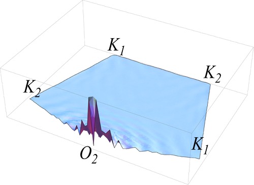


The third primitive model can be studied pictorially. Fig. 20 shows that this model harbors a MBS at its core, represented by the red open circle.
The findings for all primitive models are summarized in Table 7.
| Frank angle | |||
|---|---|---|---|
As before, we can apply the linearity of the index under the composition of systems with the same symmetry of Eq. 89 to derive its form. There is total freedom to choose linear combinations of Hamiltonians because there is no weak invariant in any -symmetric superconductor. Let us start by taking , which only has and harbors a MBS. Thus, the contribution to the index is mod 2. Now, take , and solve mod 2, to find a contribution of mod 2. Finally, take , and solve mod 2, which gives , that is, the invariant does not contribute to the index. The topological index for disclinations is then given by mod 2. The linearity of the index on the Frank angle of Eq. 88 implies that the topological index for a generic disclination with Frank angle is
| (93) |
The index is always an integer because of the constraint in Eq. 37 on the Chern and rotation invariants. There is no translation term since the weak-invariant always vanishes for symmetry.
In the search for MBS at disclinations in other 2D -wave wire systems we found that triangular lattices with second nearest-neighbor interactions do harbor MBS in disclinations; however, according to the topological invariants, these systems belong to the same class as the primitive model , which only has nearest-neighbor hopping. As shown in Fig. 21, this is because, unlike in the -symmetric second nearest-neighbor -wave wire of primitive model , the triangular sublattice that harbors the MBS does not interact with the other two triangular sublattices when the disclination is induced. On the contrary, when we considered the Kagome lattice, we found it to be topologically trivial and harboring no MBS.

V.4 Threefold symmetry
For superconductors and , which are -symmetric, the index predicts no MBS in disclinations. To corroborate this, and to investigate the third primitive generator , which breaks symmetry, all three models were simulated by putting their triangular lattices on a torus. This time, only one disclination and one disclination were necessary to compensate curvature, as shown in Fig. 22a. Just as in the case, , and only disclinations centered at vertices need to be considered, with cores as in Fig. 22b,c.
Simulations indicated that no MBS exist for any of the three models. However, when fluxes of were bound to the disclinations with Frank angles of respectively, MBS appeared in all models, and in all disclinations. Fig. 23 shows simulation results for with an extra quantum of flux added.


The findings for all primitive models are summarized in Table 8.
| Frank angle, SC flux | |||
|---|---|---|---|
| , no extra flux | |||
| , extra flux |
The results indicate that the index does not depend on either or , which is expected since the index for -symmetric systems was independent from . This, in addition to the information summarized in Table 8 leads to the index
| (94) |
for . Notice that, unlike the cases treated before, here accounts for the superconducting flux, and not the classical Frank angle of the disclination. Both can either be the same, or differ by an extra flux quantum of , as discussed in Sec. IV. The case of binding extra quanta of flux to disclinations in lattices where the order of rotation is even is treated in Appendix E. In those cases, a different rotation operator is associated with the extra flux, thus changing the rotation invariants in accordance with Eq. 21. In any case, the result amounts to an inversion of the parity of MBS whenever the Chern invariant is odd, which resembles the usual result in Ref. 29 for the parity of MBS in quantum vortices.
VI Disclination and corner Majorana bound states in real materials
The topological index that counts the MBS number parity at a disclination applies to all two-dimensional gapped crystalline superconductors described by a mean field BdG Hamiltonian. In this section, we consider two well documented materials and predict the existence of disclination or corner-bound Majorana zero modes.
VI.1 Strontium ruthenate Sr2RuO4
This material has a layered perovskite structure and can be approximated by a quasi-two-dimensional theory with a fourfold lattice rotation symmetry. It is an unconventional superconductor when K, and its superconducting order parameter shows spin-triplet -wave characteristics, which is odd under time reversal and parity. [71, 72, 73, 74] The exact nature of the pairing order has been controversial. It was postulated to be a chiral state [75] however the expected edge current [76, 77] was not detected with the predicted magnitude [78, 79, 80]. The triplet pairing was later theoretically suggested by Raghu-Kapitulnik-Kivelson in Ref. 81 to be non-chiral and predominantly generated from the quasi-one dimensional and bands instead of the two-dimensional band. More recently there is STM evidence supporting the quasi-1D non-chiral nature of the material. [82] In recent work, Majorana bound states were predicted to be present on linked dislocation lines in the 3D material due to the non-trivial weak invariants . [83]. Here we discuss the MBS number parity at disclination and/or corner defects in Sr2RuO4 using the quasi-one dimensional model proposed in Ref. 81.

The electronic band theory of the material at the Fermi energy is a controlled by the orbitals of Ruthenium. In the normal metallic phase, the quasi-two-dimensional band forms a Fermi circle while the quasi-one dimensional and bands give horizontal and vertical Fermi lines (see Fig. 24a). We will focus only on the spin triplet superconductivity of the and bands, which were predicted by Ref. 81 to be the dominant superconducting pairing, and we will ignore the effects of spin-orbit coupling. Because of the quasi-1D nature, each band is physically identical to an array of weakly coupled electron wires, which, in the presence of triplet superconductivity, become the Kitaev -wave chains [27]. The and arrays are stacked perpendicular to each other and form a fourfold rotation symmetric system. This model of Sr2RuO4 is therefore topologically equivalent to the Hamiltonian in Eq. with non-zero nearest neighbor hopping but vanishing next nearest hopping . This is pictorially represented by the Majorana tight-binding model in Fig. 7a or 24b. In reality there are weak inter-wire couplings and spin-orbit coupling which hybridize different orbitals (both the order of magnitude of of ). Although spin-orbit coupling would be essential in determining the dominant superconducting order, the topology of the BdG Hamiltonian is insensitive to these weak perturbations. On one hand, weak hybridization does not change the electronic structure at the fixed points on the Brillouin zone (in the Fermi surface of the normal metallic state the bending of the -orbital bands due to hybridization does not affect the , , and points) and therefore the bulk superconducting gap does not close. On the other hand, the rotation invariants in the superconducting state are entirely determined from the normal metallic state because the pairing only affects states at the Fermi energy, which are located away from the fixed points in the Brillouin zone. Thus, as long as there is a pairing gap, the topology of the superconductor is independent from the hybridization of -orbitals.
With this description, Sr2RuO4 does not carry a chiral edge mode. However it carries a non-trivial weak topology with index as in Eq. 39 as well as rotation symmetry protected invariants shown in Table 1. As a result, the index in Eq. 91 predicts an odd MBS number parity at a type- disclination and an even parity at a type- one (see Fig. 16a,b). Since MBS always come in pairs, the periphery of the disclination system must also carry an odd number of Majorana modes. However, the non-trivial weak topology implies the existence of an additional non-chiral gapless channel along an edge that can couple to the corner states. Luckily, surface perturbations can open a gap for the non-chiral channel, e.g., a density wave perturbation (denoted by the dashed lines in Fig. 24b), which will leave an odd number of MBS at each corner (represented by red dots). Unlike disclination MBS which are protected by the bulk energy gap, corner MBS are only weakly protected as they can escape through accidental or topological gapless edge channels. We note that since Sr2RuO4 is really a 3D material, the existence of MBS implies the existence of a channel of chiral Majorana modes propagating on disclination/corner lines in the 3D sample. We also need to restore the spin degree of freedom which implies that there will be pairs of MBS, one for each spin, which could be coupled via the spin-orbit coupling, in which case they would hybridize opening a gap.
VI.2 Doped graphene
Graphene is a two-dimensional sheet of carbon arranged on a honeycomb lattice with a symmetry. Pure graphene has a semimetallic electronic structure with Fermi energy (filling ) tuned to the degeneracy point of the four massless Dirac cones, two from spin and two from valley degrees of freedom [84]. Recently, there has been a theoretical proposal for chiral superconductivity in doped graphene with the Fermi energy set around the saddle point at (filling or ) where there is a van Hove singularity in the density of states [85]. Here we explore the possibility of disclination or corner MBS by using a mean field description of superconducting graphene derived from a model [86].

The mean field Hamiltonian is given by
| (95) |
where are electron operators at the A,B sublattice, are the three nearest neighbor displacement vectors from an A site to a B site, eV is the nearest neighbor hopping strength, is the Fermi energy at the van Hove singularity, and is the superconducting order parameter for . The pairing term involves nearest neighbor electrons, and the order parameter is proportional to
| (96) |
for -wave pairing, or
| (97) |
for -wave pairing. The -wave state preserves the rotation and mirror symmetry of graphene as it forms a trivial one dimensional irreducible representation of . The two -wave states spontaneously break threefold rotation and mirror but they can coexist and correspond to a two-dimensional irreducible representation of the point group . Both the - and -wave states break time reversal symmetry. It was theoretically suggested that the chiral combination
| (98) |

| pairing order | ||||
|---|---|---|---|---|
| -wave | 0 | 0 | 0 | 0 |
| -wave | 2 | 0 | 0 | 0 |
The -wave state is a trivial crystalline superconductor with vanishing Chern and rotation invariants. The -state is a topological superconductor with Chern number which generates two chiral Majorana edge modes (see Fig. 26b and Table 9). Since the -wave pairing breaks threefold symmetry, the superconductor is only twofold symmetric and has trivial twofold rotation invariants. Nevertheless, the index theorem in Eq. 92 still predicts an odd MBS number parity at a disclination due to the Chern number contribution. As a disclination can be decomposed into three ones, it would be natural to expect an odd MBS parity at a pentagon or heptagon defect although a sixfold rotation symmetry is absent in the BdG theory. Notice that a quantum flux vortex does not generically bind a MBS since the Chern number of the -state is even. The fact that disclinations do trap an odd number of MBS is a result of vortex fractionalization which is facilitated by the intertwining pairing and rotation order. This is remarkable because it implies that superconductors with even Chern numbers can still host an odd number of MBS on certain defects.
Notably, grain boundaries are also not uncommon in graphene. [87] One type of grain boundary is a line defect in the two-dimensional sheet formed by a series of sided plaquette defects, i.e., a chain of disclination dipoles. When pairing is formed, each defect will carry a single MBS. Thus, this type of grain boundary would serve as a realization of Kitaev’s -wave superconducting chain [27] and an alternative to proximity induced superconducting spin-orbit coupled semiconductors [46, 47, 18].
VII Discussion and Conclusions
The primary goal of this work was to provide a topological classification for 2D superconductors with discrete rotation symmetry as well as index theorems that determine the parity of Majorana bound states in composite defects composed of fluxes, dislocations and disclinations. We have found the classification to be quite rich and varied across the different rotation symmetries. Since most crystalline systems exhibit some type of 2D rotation symmetry, the results of this work can be applied to a broad class of crystalline superconductors. Interestingly we found that even in systems with an even integer or vanishing Chern number, disclination defects can bind an odd number of Majorana bound states. There are even cases when both the Chern number and weak invariants are trivial and disclinations still bind an odd number of Majorana modes due to topological rotation invariants. Thus we can find Majorana modes in non-chiral superconductors if the proper rotation invariants are non-vanishing.
In addition to the Majorana modes bound in disclinations we also discussed zero-modes that can occur at the corners of crystalline samples. The existence of corner states in fact is an exciting new way to realize Majorana modes. Another recent work discussing corner states appeared in Ref. 88 which discusses corner states in Fullerene-type crystalline arrangements. The type of corner effects discussed here are not limited to 2D and can also appear in 3D. For example, consider a 3D version of the -wave wire in a simple cubic lattice in which eight Majorana fermions are assigned to each site of the lattice, and which have third-nearest-neighbor connections, as shown in Fig. 27a. This model has a cubic BZ as shown in Fig. 27b. There are fixed points of four types: one point, three points (counting permutations of coordinate values), three points (again, with permutation of coordinate values), and one point. While we will leave the full discussion to future work, we note that the representation of the rotation is trivial at points and , but non-trivial at the point. At the point, the representation is non-trivial due to the rotation spectrum of the operator that has as an axis of rotation the line that passes by and . It is clear from the construction that by comparison to the 2D symmetric model this system will have corner states on the eight corners of a cubic sample. Since corner states could be accessed via STM probes or even just transport tunneling contacts the bound states trapped on corner defects may be observed.
While we have only considered rotation symmetries in this work it will be interesting to see what additional constraints or invariants arise when additional reflection symmetries are added. For insulators, some of these things have been discussed in Refs. 11, 12, but with the addition of particle-hole symmetry required for superconductors there may be additional complications. Also a full extension of this type of classification to superconductors with 3D point groups is also lacking. We leave these further classifications to future work.

Acknowledgements: We acknowledge useful discussions with B. Bernevig and C. Fang. J.C.Y.T. acknowledges support from the Simons Foundation Fellowship. T.L.H. was supported by ONR Grant No. N0014-12-1-0935. We also thank the support of the UIUC ICMT.
Appendix A Rotation eigenvalues and invariants
In this appendix we apply the constraints on the rotation eigenvalues described in Sec. II.1 to deduce the sets of rotation invariants for the rotation symmetries , and . The derivation of the invariants for -symmetry is found in Sec. II.1.
A.1 Twofold Symmetry
In systems with symmetry, the invariant points are , each of which has eigenvalues and as shown in Fig. 28.
Let us define the invariants
| (99) | ||||
| (100) | ||||
| (101) |
for . Due to PH symmetry and the fact that the number of occupied bands is constant over the Brillouin zone, we have
| (103) |
Twofold symmetric systems are thus characterized by their Chern number and three rotation invariants, which we choose to be
| (104) | ||||
| (105) | ||||
| (106) |

A.2 Sixfold Symmetry
In systems with symmetry, the invariant points are , and . Of these, only and are relevant, because symmetry relates to , and to and to . The corresponding eigenvalues are , , , , , and ; , , ; and , as shown in Fig. 29. Let us define the invariants
| (107) | ||||
| (108) | ||||
| (109) | ||||
| (110) | ||||
| (111) |
The fact that there is a constant number of bands over the Brillouin zone implies that
| (112) |
while the fact that there is a constant number of rotation eigenvalues over the Brillouin zone leads to
| (113) |
Therefore, in addition to the Chern number, we only need two rotation invariants to characterize the topology of symmetric systems:
| (114) | ||||
| (115) |

A.3 Threefold Symmetry
In systems with symmetry, the invariant points are . The corresponding eigenvalues are as shown in Fig. 30. Let us define the invariants
| (116) | ||||
| (117) |
for . The constant number of bands over the Brillouin zone implies that
| (118) |
while the constant number of rotation eigenvalues over the Brillouin zone leads to
| (119) |
So, in addition to the Chern number, we only need two rotation invariants to characterize the topology of symmetric systems:
| (120) | ||||
| (121) |

Appendix B Constraints on the Chern and weak invariants due to rotation symmetry
Although the relations between the Chern invariant and the rotation invariants for each of the four rotational symmetries can be inferred by the relations shown in the work of Fang et. al.[11] if PH symmetry is taken into account, here we present a detailed derivation of these relations for the sake of completeness. We do this by direct evaluation of Eq. 9 for the Chern invariant and Eq. 10 for the weak invariants.
B.1 Constraints on the Chern invariant

Consider a fundamental domain of an -fold symmetric Brillouin zone, as shown in gray in Fig. 31. The entire Brillouin zone can be generated by rotating the fundamental domain times. Let the fundamental domain be , and let us call , the domain generated by rotation of the fundamental domain times, for . Let , for , be the domain intersection with orientation depicted by the arrows in Fig. 31. There is no topological obstruction in choosing a basis of occupied states over the fundamental domain (here labels the occupied band and the subindex between parenthesis labels the domain). Similarly, in general, there is no obstruction in choosing basis states over . Therefore, defining the Berry connection on the domain as
| (122) |
the Chern invariant can be evaluated by integrating Berry curvature in the Brillouin zone which we now show reduces to an integral of the transition functions along the domain intersections :
| (123) |
where is the gauge transformation or transition function defined along the intersection :
| (124) |
Rotation symmetry implies for in ,
| (125) |
and therefore all the line integrals in Eq. 123 can be rotated back to the fundamental domain . For instance,
| (126) |
Fig. 31 shows the lines of integration. They consist of lines joining the rotation fixed points in the Brillouin zone. Given fixed points and ,
| (127) |
Crucially, the transition functions at the rotation fixed points are simply the rotation operators projected into the subspace of occupied bands
| (128) |
At these fixed points, the projected rotation operator can be diagonalized into
| (129) |
where indicates the number of occupied states at fixed point with rotation eigenvalue . Thus, we see that the line integrals of the form of Eq. 127 needed for the calculation of the Chern invariant depend ultimately on evaluations of the rotation operators at the fixed points. To be more precise, let us define the rotation index at to be
| (130) |
The Chern invariant can be related to a linear combination of such indices, one at each of the fixed points. A detailed calculation now follows for each rotation symmetry.
B.1.1 Fourfold symmetry
The Chern invariant is
| (131) |
Here, the factor of 4 is a result of the fourfold symmetry, which allows the line integrals to be rotated back to the fundamental domain by virtue of Eq. 126. and are fourfold fixed points, while and are twofold fixed points. The transition function at is exactly the fourfold rotation operator projected into the occupied bands . Similarly, . On the other hand, at , the transition functions are related to the projected twofold rotation operator by . Similarly, . Thus, the terms in Eq. 131 can be written in terms of the rotation indices
| (132) | ||||
| (133) | ||||
| (134) |
leading to the following expression for the Chern invariant
| (135) |
In terms of the rotation invariants, the relation above can be expressed as
| (136) |
B.1.2 Twofold symmetry
The Chern invariant is
| (137) |
where the factor of two arises from the twofold symmetry, which allows rotating the line integrals back to the fundamental domain. All the points in the line integral are twofold fixed points, thus for . Therefore, the Chern invariant can be written as
| (138) |
In terms of the rotation invariants, the relation above can be expressed as
| (139) |
B.1.3 Sixfold symmetry
The Chern invariant is
| (140) |
Here, is a sixfold fixed point, and are threefold fixed points related by twofold symmetry, and , , and are twofold fixed points related by threefold symmetry. The transition functions in terms of the projected rotation operators are , , and . From these relations we have
| (141) | ||||
| (142) | ||||
| (143) |
Twofold symmetry implies that and threefold symmetry implies that . Notice that the second term in the line integral for the Chern invariant involves , the transition function relating the fundamental domain and . By inserting a complete set of occupied states we have
| (144) | ||||
| (145) |
Combining the expressions above and Eq. 140 the Chern invariant is
| (146) |
In terms of the rotation invariants
| (147) |
B.1.4 Threefold symmetry
The Chern invariant is
| (148) |
Here all points are threefold fixed points, and the rotation operators are for . Thus, the Chern number is equal to
| (149) |
In terms of the rotation invariants
| (150) |
B.2 Constraints on the weak invariants

Consider determining the weak invariant in a twofold symmetric crystal. Following the notation in Fig. 32 for the fixed points, the line integral of the Berry connection along the boundary is
| (151) |
The first term in Eq. 151, which integrates along the lower-right half of the BZ boundary, will be written as an integral along its upper-left half boundary (dashed lines in Fig. 32). This is possible since the connection can be written as
| (152) |
where we have made use of the gauge change . This allows us to relate the integral to the rotation invariants as follows:
| (153) |
which, in terms of the rotation invariants, can be written as
| (154) |
Similarly, we find
| (155) |
In fourfold symmetric crystals the calculation follows the same steps. The twofold rotation of the first term in Eq. 151 amounts to a double application of the fourfold rotation operator , which results in the index
| (156) |
or, in terms of the rotation invariants
| (157) |
In symmetric crystals, . This is because under threefold rotation the reciprocal lattice vectors and change according to , and , and symmetry demands that , which implies that and , or mod 2. Thus, .
Appendix C Proof that the stable classification of TCS is complete
In this Appendix we complete the proof we delayed from Sec. III. First, consider two Hamiltonians and with the same . We can match their rotation eigen-spectra and second-descendant invariants simply by the addition of trivial bands. Next, the energy spectrum of and can be flattened to take away any dispersion, i.e. . Our aim then is to deform into over all values of in the fundamental domain of the Brillouin zone (gray zones in Fig. 2), and rotation symmetry will guarantee that this deformation applies for values of over the entire Brillouin zone. For demonstration we choose a symmetric system with the fundamental domain being a square. A deformation is equivalent to a Hamiltonian defined on the cube in Fig. 33 with fixed boundary Hamiltonians and .

To prove the existence of a continuous deformation, one proceeds by showing that there is no obstruction to a continuous interpolation in the cube in Fig. 33 starting with the edges, then the faces, and finally the full volume.
(i) At a point in momentum space that remains invariant under rotation, the Hamiltonians can be deformed into each other as the rotation representations and the second-descendant invariants for and are identical. Therefore, there is a deformation along the edges of the cube.
(ii) Next we fill in the faces. For demonstration, consider the front face . The deformation Hamiltonian is already fixed along the boundary by procedure (i). For a -symmetric system, belongs to class A as is not closed under PH symmetry. For a -symmetric system with a twofold symmetry , belongs to class C with the combined PH symmetry that squares to minus one. The new PH operator fixes both momentum and the deformation parameter
| (158) |
The topological classification of such a system falls in the classification of topological defects in Ref. 56. The relevant defect dimension is given by , where counts the dimension of parameters odd under the symmetry and is the dimension for even ones. Along the face boundary , all parameters are even under and therefore the “defect” dimension is (which is 7 mod 8). There are no non-trivial classifications for both classes A and C. is therefore topologically trivial, and there is no obstruction in extending the deformation Hamiltonian over the whole face . Note that this also defines the Hamiltonian on other faces that are related to by rotation. In Fig. 33 for instance, the face is related to by a rotation.
(iii) Finally we fill in the rest of the volume for the deformation Hamiltonian. From (i) and (ii), has already been fixed along the boundary . Similar to the previous procedure, depending on whether there is a symmetry, belongs to either class A or class C with the new PH symmetry of Eq. 158. The “defect” dimension on the surface is (or 6 mod 8), and is integrally topologically classified by the Chern invariant [56] . However, the Berry curvatures cancel each other between different faces. For example, in Fig. 33, the curvatures over faces and annihilate as the two are related by symmetry but with opposite orientations (one facing in the cube and the other facing out). The curvatures along the top and bottom faces also cancel out since the two systems are assumed to have identical Chern invariant and the two faces again have opposite orientation with respect to the cube. The vanishing of the Chern invariant implies is trivial along the boundary surface . Equivalently there is no “monopole” in the volume and the deformation Hamiltonian can be extended all the way inside.
Appendix D Lattice cell construction for simulations of disclinations in chiral primitive models
Here we describe in detail the construction of the lattice cells for the simulation of the spinless chiral primitive models. We first consider the generation of an disclination in a symmetric lattice as an illustrating example. Inducing a disclination can be achieved by means of the Volterra process, shown in Fig. 34. For this purpose, one divides the lattice into four quadrants and removes the fourth one. The space created is then filled by stretching the remaining quadrants around the center point.


Let us assign a frame to each quadrant in such a way that their axes rotate by counter-clockwise from one quadrant to the next. Generating the disclination distorts the primitive vectors of the lattice , for , defined with respect to each frame in quadrant , which thus become position dependent. The distorted vectors are related to the original lattice vectors by a position-dependent rotation
| (159) |
For example, for the uniform angular stretching shown in Fig. 34, the rotation is , where is the azimuthal angle in the plane measured before the deformation from the frame axis . Take, for example, ; after the deformation we have , that is, there is a complete filling of the region left after the removal of the fourth quadrant (see Fig. 34c).

To capture the effect of this distortion in the crystal, consider a Hamiltonian with nearest-neighbor pairing and hopping terms in real space
| (160) |
Here runs over lattice sites within quadrant , and act on the Nambu degree of freedom, and for are the distorted primitive lattice vectors in quadrant .
While the hopping terms are unaffected by the disclination, the pairing terms effectively pick up a fractional superconducting flux centered at its core, because
| (161) |
where is the rotated superconducting order parameter, which partially winds around the disclination.
In our simulations we must accommodate multiple disclinations to use lattice cells with periodic boundary conditions. All three lattice cells shown in Figs. 14, 18 and 22 were decomposed into quadrants, as shown in Fig. 36. To each of these quadrants a rotation function was assigned, where smoothly winds the order parameter around its corners but has zero winding overall, as shown in Fig. 35. By using this function at each of the quadrants in Fig. 36, disclinations are created at each of the quadrant’s vertices, with opposite winding at adjacent vertices, and which still allow for periodic boundary conditions to be imposed on the lattice cells. The values of the total phase winding at each corner of the quadrant were chosen so that the total winding around the disclinations matches its Frank angle , i.e., so that , where is the number of quadrant’s corners that meet at each disclination.
Appendix E Energy scaling signatures of MBS and the incidence of binding an extra flux quantum to disclinations
Obtaining wavefunctions for low-energy modes localized at disclination cores is not sufficient to infer the presence of MBS because the (fractional) superconducting fluxes at disclinations can bind other non-Majorana modes which might still lie at low-energy and appear localized. Additionally, since multiple disclinations exist in any of the simulated lattice cells, and since if MBS are present they must come in pairs, we must examine the exponential decay of the energy splitting of the low-energy modes as a function of their separation as a conclusive criterion for their existence. In this Appendix we show the energy scaling plots as a function of system size (and therefore disclination separation) which justifies our claims on the existence of MBS. We show these scaling plots for all the primitive models discussed in this paper.
In addition to this, we present the scaling plots for models to which an additional flux quantum was bound to disclinations. Recall that the for fermionic systems the rotation operator is lifted to its double cover. As a result, a rotation operator , parameterized by , exists, which is inequivalent to . This other operator is equivalent to having an extra superconducting flux quantum () bound to the disclination. The inequivalence of these operators is exemplified in different rotation invariants for the same Hamiltonian matrix, which are modified according to Eq. 21. In -symmetric systems, this amounts to an exchange of the rotation invariants , while in symmetric systems, all rotation invariants flip sign. In both cases, the weak index remains unaffected. In -symmetric systems, a flip in the sign of takes place. We verified in simulations that, after these changes in the invariants, the parities of MBS are given by the same indices derived in Sec. V.
The MBS parities for the and primitive models are shown in Tables 11 and 11. In the upper half of each of these tables we have reproduced the results in Tables 5 and 6 of Sec. V. The lower half of each of these tables shows the results for lattices with extra flux quanta at their disclinations. For the models and these parities were inferred from the scaling argument explained above. Fig. 37 shows the energy scaling for the cases in which MBS were found (the plots are not shown; since the chiral primitive models are the same for and symmetries, the scaling plots for the case are redundant).
| phase winding, type | ||||
|---|---|---|---|---|
| , type-(0,0) | ||||
| , type-(1,0) | ||||
| , type-(0,0) | ||||
| , type-(1,0) |
| phase winding, type | ||||
|---|---|---|---|---|
| , type-(0,0) | ||||
| , type-(1,0) | ||||
| , type-(0,1) | ||||
| , type-(1,1) | ||||
| , type-(0,0) | ||||
| , type-(1,0) | ||||
| , type-(0,1) | ||||
| , type-(1,1) |
The MBS parities for the and primitive models with and without extra flux quantum are shown in Tables 12 and 13. Except for primitive model , all primitive generators in these symmetries are models, and their parities were inferred from the scaling plots shown in Figs. 39 and 40, which plot the absolute value of the energy for the lowest eigenstates as a function of system size . The signature of MBS consist of energies that exponentially tend to zero as the system size increases. We point out that in the case of Figs. 39c,f, the model is not a primitive generator (recall that is a 2D -wave wire model, whose MBS parity was determined pictorially in Fig. 20), but rather, an additional model that we have considered to illustrate the linearity of the topological indices for the parity of MBS. This extra model has third nearest-neighbor hopping terms added to the Hamiltonian in Eq. 66. When these terms are added, two other phases appear apart from those in Fig. 8, as shown in Fig. 38. The phase with is trivial, as it has , while the phase with is in the non-trivial class . This last Hamiltonian, which we call , is the one shown in Figs. 39c,f. This model is topologically equivalent to . Therefore, the MBS parity for this model is given by mod 2, which gives an odd number of MBS with and without an extra flux quantum, as verified in the energy scaling observed in Figs. 39c,f.
| phase winding | |||
|---|---|---|---|
| phase winding | |||
|---|---|---|---|
In all of these models, adding an extra flux quantum flipped the parity of MBS only when the model has an odd Chern invariant, following the result in Ref. 29. This is consistent with the -wave wire primitive models not changing the parity upon addition of an extra flux quantum, since they have , which is indeed what we would expect for models whose MBS parity can be determined pictorially.
References
- [1] M. Z. Hasan and C. L. Kane, Rev. Mod. Phys. 82, 3045 (2010).
- [2] X.-L. Qi and S.-C. Zhang, Rev. Mod. Phys. 83, 1057 (2011).
- [3] C. L. Kane and E. J. Mele, Phys. Rev. Lett. 95, 226801 (2005a).
- [4] J. C. Y. Teo, L. Fu, and C. L. Kane, Phys. Rev. B 78, 045426 (2008).
- [5] A. M. Turner, Y. Zhang, R. S. Mong, and A. Vishwanath, Phys. Rev. B 85, 165120 (2012).
- [6] T. L. Hughes, E. Prodan, and B. A. Bernevig, Phys. Rev. B 83, 245132 (2011).
- [7] C.-K. Chiu, H. Yao, and S. Ryu, Phys. Rev. B 88, 075142 (2013).
- [8] Y. Ueno, A. Yamakage, Y. Tanaka, and M. Sato, Phys. Rev. Lett. 111, 087002 (2013).
- [9] F. Zhang, C. L. Kane, and E. J. Mele, Phys. Rev. Lett. 111, 056403 (2013).
- [10] L. Fu, Phys. Rev. Lett. 106, 106802 (2011).
- [11] C. Fang, M. J. Gilbert, and B. A. Bernevig, Phys. Rev. B 86, 115112 (2012).
- [12] C. Fang, M. J. Gilbert, and B. A. Bernevig, Phys. Rev. B 87, 035119 (2013).
- [13] J. C. Y. Teo and T. L. Hughes, Phys. Rev. Lett. 111, 047006 (2013).
- [14] R.-J. Slager, A. Mesaros, V. Juričić, and J. Zaanen, Nat. Phys. 9, 98 (2012).
- [15] E. Majorana, Nuovo Cimento 5, 171 (1937).
- [16] F. Wilczek, Nat. Phys 5, 614 (2009).
- [17] C. W. J. Beenakker, Annu. Rev. Con. Mat. Phys. 4, 113 (2013).
- [18] J. Alicea, Rep. Prog. Phys 75, 076501 (2012).
- [19] D. A. Ivanov, Phys. Rev. Lett. 86, 268 (2001).
- [20] A. Kitaev, Ann. Phys. 321, 2 (2006).
- [21] A. Kitaev, Ann. Phys. 303, 2 (2003).
- [22] R. W. Ogburn and J. Preskill, Comp. Sci. 1509, 341 (1999).
- [23] J. Preskill, Topological quantum computation (2004), URL http://www.theory.caltech.edu/people/preskill/ph229/#lecture.
- [24] M. Freedman, A. Kitaev, M. Larsen, and Z. Wang, arXiv:quant-ph/0101025 (2001).
- [25] C. Nayak, S. H. Simon, A. Stern, M. Freedman, and S. Das Sarma, Rev. Mod. Phys. 80, 1083 (2008).
- [26] Z. Wang, Topological Quantum Computation (American Mathematics Society, 2010).
- [27] A. Y. Kitaev, Phys.-Usp. 44, 131 (2001).
- [28] G. E. Volovik, Pisma Zh. Eksp. Teor. Fiz. 70, 601 (1999).
- [29] N. Read and D. Green, Phys. Rev. B 61, 10267 (2000).
- [30] M. Sato, and S. Fujimoto, Phys. Rev. B 79, 094504 (2009).
- [31] N. Read and G. Moore, Nucl. Phys. B 360, 362 (1991).
- [32] M. Greiter, X.-G. Wen, and F. Wilczek, Nucl. Phys. B 374, 567 (1992).
- [33] C. Nayak and F. Wilczek, Nucl. Phys. B 479, 529 (1996).
- [34] C. L. Kane and E. J. Mele, Phys. Rev. Lett. 95, 146802 (2005b).
- [35] M. König, S. Wiedmann, C. Brüne, A. Roth, H. Buhmann, L. Molenkamp, X.-L. Qi, and S. Zhang, Science 318, 766 (2007).
- [36] J. E. Moore and L. Balents, Phys. Rev. B 75, 121306(R) (2007).
- [37] R. Roy, Phys. Rev. B 79, 195322 (2009).
- [38] L. Fu, C. L. Kane, and E. J. Mele, Phys. Rev. Lett. 98, 106803 (2007).
- [39] X.-L. Qi, T. L. Hughes, and S.-C. Zhang, Phys. Rev. B 78, 195424 (2008).
- [40] D. Hsieh, D. Qian, L. Wray, Y. Xia, Y. S. Hor, R. J. Cava, and M. Z. Hasan, Nature 452, 970 (2008).
- [41] L. Fu and C. L. Kane, Phys. Rev. Lett. 100, 096407 (2008).
- [42] A. R. Akhmerov, J. Nilsson, and C. W. J. Beenakker, Phys. Rev. Lett. 102, 216404 (2009).
- [43] L. Fu and C. L. Kane, Phys. Rev. Lett. 102, 216403 (2009).
- [44] K. T. Law, P. A. Lee, and T. K. Ng, Phys. Rev. Lett. 103, 237001 (2009).
- [45] J. R. Williams, A. J. Bestwick, P. Gallagher, S. S. Hong, Y. Cui, A. S. Bleich, J. G. Analytis, I. R. Fisher, and D. Goldhaber-Gordon, Phys. Rev. Lett. 109, 056803 (2012).
- [46] J. D. Sau, R. M. Lutchyn, S. Tewari, and S. Das Sarma, Phys. Rev. Lett. 104, 040502 (2010).
- [47] Y. Oreg, G. Refael, and F. von Oppen, Phys. Rev. Lett. 105, 177002 (2010).
- [48] V. Mourik, K. Zuo, S. Frolov, S. Plissard, E. Bakkers, and L. Kouwenhoven, Science 336, 1003 (2012).
- [49] X. Liu, and K. T. Law, arxiv.org/abs/1310.5685 (2013).
- [50] C. Fang, M. J. Gilbert, and B. A. Bernevig, arxiv.org/abs/1308.2424 (2014).
- [51] M. Sato, Y. Yakahashi, and S. Fujimoto, Phys. Rev. Lett. 103, 020401 (2009).
- [52] X.-G. Wen, Int. J. Mod. Phys. B 4, 239 (1990).
- [53] X.-G. Wen, Quantum Field Theory of Many Body Systems (Oxford Univ. Press, Oxford, 2004).
- [54] E. Fradkin, Field Theories of Condensed Matter Physics (Cambridge University Press, 2013), second ed.
- [55] J. C. Y. Teo and C. L. Kane, Phys. Rev. Lett. 104, 046401 (2010a).
- [56] J. C. Y. Teo and C. L. Kane, Phys. Rev. B 82, 115120 (2010b).
- [57] A. A. Abrikosov, Sov. Phys. JETP 5, 1174 (1957).
- [58] Y. Ran, Y. Zhang, and A. Vishwanath, Nat. Phys 5, 298 (2009).
- [59] Y. Ran, arXiv:1006.5454 (2010).
- [60] D. Asahi and N. Nagaosa, Phys. Rev. B 86, 100504(R) (2012).
- [61] V. Juricic, A. Mesaros, R.-J. Slager, and J. Zaanen, Phys. Rev. Lett. 108, 106403 (2012).
- [62] A. Altland and M. R. Zirnbauer, Phys. Rev. B 55, 1142 (1997).
- [63] A. P. Schnyder, S. Ryu, A. Furusaki, and A. W. W. Ludwig, Phys. Rev. B 78, 195125 (2008).
- [64] A. Kitaev, AIP Conf. Proc. 1134, 22 (2008).
- [65] M. Karoubi, K-theory: An introduction, vol. 226 (Springer, 2008).
- [66] N. D. Mermin, Rev. Mod. Phys. 51, 591 (1979).
- [67] P. M. Chaikin and T. C. Lubensky, Principles of Condensed Matter Physics (Cambridge University Press, 2000).
- [68] D. R. Nelson, Defects and Geometry in Condensed Matter Physics (Cambridge University Press, 2002).
- [69] M. Kleman and J. Friedel, Rev. Mod. Phys. 80, 61 (2008).
- [70] S. Gopalakrishnan, J. C. Y. Teo, and T. L. Hughes, Phys. Rev. Lett. 111, 025304 (2013).
- [71] G. M. Luke, Y. Fudamoto, K. M. Kojima, M. I. Larkin, J. Merrin, B. Nachumi, Y. J. Uemura, Y. Maeno, Z. Q. Mao, Y. Mori, et al., Nature 394, 558 (1998).
- [72] K. D. Nelson, Z. Q. Mao, Y. Maeno, and Y. Liu, Science 306, 1151 (2004).
- [73] F. Kidwingira, J. D. Strand, D. J. Van Harlingen, and Y. Maeno, Science 314, 1267 (2006).
- [74] J. Xia, Y. Maeno, P. T. Beyersdorf, M. M. Fejer, and A. Kapitulnik, Phys. Rev. Lett. 97, 167002 (2006).
- [75] T. M. Rice and M. Sigrist, J. Phys.: Condens. Matter 7, L643 (1995).
- [76] M. Matsumoto and M. Sigrist, J. Phys. Soc. Jpn. 68, 994 (1999).
- [77] M. Stone and R. Roy, Phys. Rev. B 69, 184511 (2004).
- [78] P. G. Bjornsson, Y. Maeno, M. E. Huber, and K. A. Moler, Phys. Rev. B 72, 012504 (2005).
- [79] J. R. Kirtley, C. Kallin, C. W. Hicks, E.-A. Kim, Y. Liu, K. A. Moler, Y. Maeno, and K. D. Nelson, Phys. Rev. B 76, 014526 (2007).
- [80] C. W. Hicks, J. R. Kirtley, T. M. Lippman, N. C. Koshnick, M. E. Huber, Y. Maeno, W. M. Yuhasz, M. B. Maple, and K. A. Moler, Phys. Rev. B 81, 214501 (2010).
- [81] S. Raghu, A. Kapitulnik, and S. A. Kivelson, Phys. Rev. Lett. 105, 136401 (2010).
- [82] I. A. Firmo, S. Lederer, C. Lupien, A. P. Mackenzie, J. C. Davis, and S. A. Kivelson, arXiv:1308.0894 (2012).
- [83] T. L. Hughes, H. Yao, and X.-L. Qi, arXiv:1303.1539 (2013).
- [84] A. H. Castro Neto, F. Guinea, N. M. R. Peres, K. S. Novoselov, and A. K. Geim, Rev. Mod. Phys. 81, 109 (2009).
- [85] R. Nandkishore, L. S. Levitov, and A. V. Chubukov, Nature Physics 8, 158 (2012).
- [86] A. M. Black-Schaffer and S. Doniach, Phys. Rev. B 75, 134512 (2007).
- [87] P. Y. Huang, C. S. Ruiz-Vargas, A. M. van der Zande, W. S. Whitney, M. P. Levendorf, J. W. Kevek, S. Garg, J. S. Alden, C. J. Hustedt, Y. Zhu, et al., Nature 469, 389 (2011).
- [88] A. Rüegg, S. Coh, and J. E. Moore, Phys. Rev. B 88, 155127 (2013).