Functional Factorial $K$-means Analysis

First we present the notation that we will use throughout this paper. Here, the same notations as Yamamoto (2012) will be used for ease of explanation. Suppose that the $n$th functional object ($n=1,\dots,N$) with $P$ variables is represented as $x_{n}(t)=(x_{np}(t)\mid p=1,\dots,P)$ with a domain $T\subset\mathbb{R}^{d}$. For simplicity, we write $x_{n}=(x_{n}(t)\mid t\in T)$ to denote the $n$th observed function. In the rest of paper, for general understanding of the problem, we consider the single-variable case, i.e., $P=1$; in this case, the suffix $p$ in the above notation will be omitted. The multivariate case will be described in Appendix A. Let $\mathscr{L}=L^{2}(T)$, which is the usual Hilbert space of function $f$ from $T$ to $\mathbb{R}$. Here, the inner product for any $x,y\in\mathscr{L}$ is defined as

and for any $x\in\mathscr{L}$, $\|x\|:=\left<x,x\right>^{1/2}<\infty$.

For simplicity, we shall assume that the mean function of the $x_{n}$’s has been subtracted, so without loss of generality, we assume that $\sum_{n=1}^{N}x_{n}(t)=0$ for all $t\in T$.

In this paper, we simultaneously find an optimal projection of the data $\boldsymbol{x}=(x_{1},\cdots,x_{N})^{\prime}$ into a low-dimensional subspace and a cluster structure. Let $V=\{v_{l}\}$ $(l=1,\dots,L<\infty;\;v_{l}\in\mathscr{L})$ be orthonormal basis functions of the projected low-dimensional subspace. In this paper, as with Yamamoto (2012), we call $v_{l}$ a weight function. In addition, let $\mathtt{P}_{v}$ be an orthogonal projection operator from the functional data space $\mathscr{L}$ onto the subspace $\mathscr{S}_{v}$, which is spanned by $V$. Let $U=(u_{nk})_{N\times K}$ be cluster assignment parameters, where $u_{nk}$ equals one if subject $n$ belongs to cluster $k$, and zero, otherwise. Let $N_{k}$ be the number of subjects that are assigned to the $k$th cluster, and for all $k$, $\bar{x}_{k}:=N_{k}^{-1}\sum_{n=1}^{N}u_{nk}x_{n}$, which is the centroid of the $k$th cluster. In this paper, we consider crisp clustering, in which each object is assigned to only one group.

A basis function expansion approach is used in many functional data analysis models. Let us approximate an object $x_{n}$ using a basis function, as follows

where $\phi_{m}$’s $(m=1,\dots,M)$ are basis functions (e.g., Fourier or B-spline basis functions) and $g_{nm}$ is a coefficient corresponding to $(x_{n},\phi_{m})$, and we write $\boldsymbol{\phi}=(\phi_{1},\dots,\phi_{M})^{\prime}$ and $\boldsymbol{g}_{n}=(g_{n1},\cdots,g_{nM})^{\prime}$. Then, we have

Similarly, the weight functions described above are expanded by the same basis functions,

where $\boldsymbol{a}_{l}=(a_{l1},\cdots,a_{lM})^{\prime}$. Then, we also have

Let $\mathbf{H}$ be an $M\times M$ matrix that has $\left<\phi_{i},\phi_{j}\right>$ for the $ij$th element. Furthermore, let $\mathbf{G}_{H}=\mathbf{G}\mathbf{H}^{\frac{1}{2}}$, and $\mathbf{A}_{H}=\mathbf{H}^{\frac{1}{2}}\mathbf{A}$.

As described previously, the clustering method with dimension reduction can produce useful information about the cluster structure that exists in functional data. To attain this purpose, the functional principal component $k$-means (FPCK) method has been proposed (Yamamoto, 2012), and this method succeeds in extracting a cluster structure that provides useful information. However, the FPCK method has a drawback. A typical example in which the FPCK analysis does not perform well is given as follows:

This failure of the FPCK method can be explained through the decomposition of its loss function. The loss function $L_{fpck}$ of the FPCK method has the following decomposition:

If we use basis function expansions of the data and weight functions, $L_{fpck}$ is approximated as

where $\mathbf{P}_{U}$ is a projection matrix onto the space spanned by the columns of $\mathbf{U}=(u_{nk})$. The first term of the right-hand side measures the distance between the coefficient matrix $\mathbf{G}_{H}$ and the projection of $\mathbf{G}_{H}$ onto the subspace spanned by the columns of $\mathbf{A}_{H}$. That is, this term determines the degree of the dimension reduction of the data. On the other hand, the second term measures the distance between the projection of $\mathbf{G}_{H}$ and the centroid of clusters in the subspace. Based on this formulation, it is found that there are some cases where FPCK analysis does not work well. We illustrate this using a concrete example.

As with Example 1, consider that an $N\times M$ coefficient matrix $\mathbf{G}_{H}$ consists of two parts, $\mathbf{G}_{H}=(\mathbf{G}_{1},\mathbf{G}_{2})$, where $\mathbf{G}_{1}$ is an $N\times M_{1}$ matrix that is related to the cluster structure, and $\mathbf{G}_{2}$ is an $N\times M_{2}$ matrix ($M=M_{1}+M_{2}$) that is independent of the cluster structure. Usually, $N$ denotes the sample size, and $M$ is the number of basis functions. If $\mathbf{G}_{1}$ has no substantial correlations, then FPCK analysis is likely to provide a different subspace from that spanned by the true $\mathbf{A}_{H}$. This is mainly because $\mathbf{G}_{1}$ is full rank, and the first term of the decomposition may be minimized by weight functions which are different from true ones. It can be inferred that when $\mathbf{G}_{1}$ is full rank, the FPCK method gets worse with an increase in the column size of $\mathbf{G}_{2}$. Evidently, it can be seen that, if the contributing part $\mathbf{G}_{1}$ to the cluster structure has no substantial correlations and the masking part $\mathbf{G}_{2}$ substantially exists, the FPCK method may fail to find the true cluster structure.

To overcome the drawback of FPCK analysis discussed above, we propose a new clustering method with dimension reduction. The notation and settings were explained in Section 2. For ease of explanation, we first consider the case in which there is only one variable, i.e., $P=1$. Thus, in this section, the suffix $p$ is omitted from the notation. An extension to the multivariate model is straightforward and is described in Appendix A.

A least-squares objective function for the proposed approach, in which the first few principal components of the data are defined to be the most informative about the cluster structure, is

This criterion is optimized over the projected space $V$ and the cluster parameter $U$.

Here, a component score $f_{nl}$ of subject $n$ for the $l$th component is defined as $f_{nl}=\langle x_{n},v_{l}\rangle$ using the estimated weight function $v_{l}$. Analysis for the first few estimated component scores $\{f_{nl}\}$ $(l=1,\dots,L)$, where $L$ is two or three, seems to be helpful for the interpretation of a cluster structure in functional data.

This approach, minimizing the objective function in (4) with respect to $V$ and $U$ simultaneously, is called the functional factorial $k$-means (FFKM) method because this method is a direct extension of the factorial $k$-means method (Vichi and Kiers, 2001) to the model for the functional setting. The loss function (4) is equivalent to the second term of the decomposition (3) of the loss function of FPCK. It might be expected that we can resolve the problem of FPCK by ruling out the first term in Eq. (3). Note that this loss function (4) was shortly referred in Yamamoto (2012).

We now present an efficient algorithm for this approach. As in the FPCK method, the criterion (4) can be optimized using the alternating least squares (ALS) approach, as follows.

1. STEP1.

   Initialize parameter $V$ subject to the restriction mentioned above.

2. STEP2.

   Minimize the loss function in Eq. (4) for fixed $V$ over $U$.

3. STEP3.

   Minimize the loss function in Eq. (4) for fixed $U$ over $V$.

4. STEP4.

   Go to STEP2, or stop.

There are two parts to the algorithm. The first part of the above ALS algorithm is to minimize $L_{ffkm}$ for fixed $V$ over $U$. To solve the optimization problem, we use a basis function expansion technique described in Section 2. If a projected object $\mathtt{P}_{v}x_{n}$ is expanded using some basis function, that is, $\mathtt{P}_{v}x_{n}=\boldsymbol{d}^{\prime}_{n}\boldsymbol{\phi}$ where $\boldsymbol{d}_{n}=(d_{n1},\dots,d_{nM})^{\prime}$, then the criterion (4) can be written as

where $\bar{\boldsymbol{d}}_{k}$ is a coefficient vector corresponding to the basis function expansion of the projected mean function $\bar{x}_{k}$ of the $k$th cluster, and $\|\cdot\|_{\mathbf{H}}$ means the Euclidean norm with the metric $\mathbf{H}$, i.e., for $\mathbf{y}\in\mathbb{R}^{M},\;\|\boldsymbol{y}\|_{\mathbf{H}}^{2}=\boldsymbol{y}^{\prime}\mathbf{H}\boldsymbol{y}$. Thus, Eq. (5) can be minimized using the usual $k$-means algorithm (Lloyd, 1982) for $\mathbf{H}^{\frac{1}{2}}\boldsymbol{d}_{n}$. Using the expansions in Eq. (2), it is found that $\mathbf{H}^{\frac{1}{2}}\boldsymbol{d}_{n}=\mathbf{A}_{H}\mathbf{A}_{H}^{\prime}\boldsymbol{g}_{Hn}$.

The second part is to minimize $L_{ffkm}$ regarding $V$. The objective function in Eq. (4) can be written as (see Yamamoto, 2012, p.246)

where $\mathtt{F}$ is an integral operator defined as, for any $y\in\mathscr{L}$,

Note that it is easily verified that the integral operator $\mathtt{F}$ is a Hilbert-Schmidt integral operator. Thus, $\mathtt{F}$ is a compact operator. In addition, $\mathtt{F}$ is clearly self-adjoint. Minimizing the criterion is, therefore, equivalent to solving the following eigenvalue equation (see, for example, Dunfort and Schwartz, 1988),

for $l=1,\dots,L$, where $\delta_{ll^{\prime}}$ is the Kronecker delta. Each eigenfunction $\{\xi_{l}\}$ $(l=1,\dots,L)$ corresponds to a weight function $\{v_{l}\}$ $(l=1,\dots,L)$, which is to be estimated. As with the first part of the ALS algorithm, to solve this eigenvalue problem, we use the basis function expansion. Then, $\mathtt{F}$ operates on a function $\xi_{l}$ as

Eventually, solving the eigenvalue problem (7) amounts to solving the eigenvalue problem

where $\boldsymbol{a}_{Hl}=\mathbf{H}^{\frac{1}{2}}\boldsymbol{a}_{l}$. The eigenfunction $\xi_{l}$ is given by the estimated eigenvector $\boldsymbol{a}_{Hl}$ as the approximation in Eq. (2) using $\boldsymbol{a}_{l}=\mathbf{H}^{-\frac{1}{2}}\boldsymbol{a}_{Hl}$.

The above ALS algorithm monotonically decreases the loss function $L_{ffkm}$ and the loss function is bounded from below. Then this algorithm guarantees the convergence to a certain point; but it may not be the global minimum. Also, in general, the $k$-means algorithm, which is utilized in the ALS algorithm, is sensitive to local optima (Steinley, 2003). Thus, to safeguard against those local minima, the proposed algorithm needs to be repeated with a number of random initial starts for $V$.

In this section, we propose a smoothing method for the FFKM model. Generally, if the functional data can be assumed to be sufficiently smooth, the analysis method considering the smoothness of functions often provides better results (see, for example, Ramsay and Silverman, 2005). Specifically, several smoothing approaches to FPCA have been developed (Rice and Silverman, 1991; Silverman, 1996; Reiss and Ogden, 2007) and investigated theoretically (Pezzulli and Silverman, 1993; Silverman, 1996; Ocana et al., 1999; Reiss and Ogden, 2007), from the beginning during the early stages of research on functional data analysis.

In this section, the FFKM method is extended to the regularized model which takes into consideration the smoothness of functional objects and weight functions. Here a regularized model for univariate is described, while the method for a multivariate case is described in Appendix A. The proposed approach to the regularized FFKM model is similar to the approach in penalized FPCA proposed by Silverman (1996).

Let $\mathtt{D}^{2}$ be the second-order differential operator, and let $\mathtt{S}^{2}_{\lambda}$ be the usual spline smoothing operator (see, Green and Silverman, 1994) with a roughness penalty $\lambda$. That is, for any function $f\in\mathscr{L}$, the loss function $\|f-g\|^{2}+\lambda\|\mathtt{D}^{2}g\|^{2}$ with the penalty of function $g$ is minimized when setting $g=\mathtt{S}_{\lambda}^{2}f$. We consider the inner product space $(\mathscr{L},\langle\cdot,\cdot\rangle_{\lambda})$ with the inner product $\left<\cdot,\cdot\right>_{\lambda}$ which is defined as, for $x,y\in\mathscr{L}$,

Note that the norm $\|\cdot\|_{\lambda}$ is given by the inner product, i.e., $\|x\|_{\lambda}=\langle x,x\rangle_{\lambda}^{1/2}$. Then, smoothed weight functions $V$ can be obtained by the FFKM method on the smoothed functional data $\mathtt{S}_{\lambda}^{2}x_{n}\;(n=1,\dots,N)$. Thus, a loss function of the regularized FFKM method is

The parameters $U$ and $V$, which minimize $L_{ffkm}(U,V)$, are estimated using an ALS algorithm similar to that for the non-regularized FFKM method, though there are two differences between the two models: in the regularized model, the inner product $\left<\cdot,\cdot\right>_{\lambda}$ is used and the smoothed data $\mathtt{S}_{\lambda}x_{n}$ is expanded. Let $\boldsymbol{g}_{\lambda,n}$ be a vector with length $M$ containing coefficients corresponding to the basis function expansion of $\mathtt{S}_{\lambda}^{2}x_{n}$, and let $\mathbf{H}_{\lambda}$ be an $M\times M$ matrix in which the $ij$th element is $\langle\phi_{i},\phi_{j}\rangle_{\lambda}$. Furthermore, let $\mathbf{A}_{H_{\lambda}}=\mathbf{H}_{\lambda}^{\frac{1}{2}}\mathbf{A}$ and $\mathbf{W}=\mathbf{H}_{\lambda}^{\frac{1}{2}}\mathbf{A}_{H_{\lambda}}\mathbf{A}_{H_{\lambda}}^{\prime}\mathbf{H}_{\lambda}^{\frac{1}{2}}$. Then, in STEP2 of the ALS algorithm, the optimal $U$ is obtained by minimizing the following criterion for fixed $V$ over $U$:

where $\|\cdot\|_{\mathbf{W}}$ is the Euclidean norm with metric $\mathbf{W}$. Thus, as with the non-regularized model, this criterion will be optimized using the usual $k$-means algorithm for $\mathbf{A}_{H_{\lambda}}\mathbf{A}_{H_{\lambda}}^{\prime}\boldsymbol{g}_{H_{\lambda}n}$.

Next, we describe how to estimate the weight functions $V$ in STEP3. Using the above basis function expansion to estimate the optimal $V$, the following eigenvalue problem is considered:

where $\boldsymbol{a}_{H_{\lambda}l}$ is the $l$th column of $\mathbf{A}_{H_{\lambda}}$. Then, as in the non-regularized method, the smoothed weight function $v_{l}$ is approximated as $v_{l}\approx\boldsymbol{\phi}^{\prime}\mathbf{H}_{\lambda}^{-\frac{1}{2}}\boldsymbol{a}_{H_{\lambda}l}$.

A component score $f_{nl}$ can be defined as that for the FFKM method, $f_{nl}=\langle x_{n},v_{l}\rangle$. Before the regularized FFKM method is applied to the data, the value of the smoothing parameter $\lambda$ should be determined. Some general remarks about the use of automatic methods for choosing smoothing parameters are found in Green and Silverman (1994) and Wahba (1990). A more detailed explanation of determining the value of $\lambda$ is presented in the next section.

Prior to applying the above algorithm, we need to determine the values of parameters: the smoothness of the basis functions, the number of clusters, and the dimensionality of the subspace. Here, we discuss in detail how these selections should be made.

First, we discuss the selection of the smoothness of the function. As described in Ramsay and Silverman (2005), it is often adequate for many purposes to choose the smoothing parameter subjectively. On the other hand, selecting the value of $\lambda$ in an automatic manner may be required if there is no prior information on the smoothness. There are two major approaches to the automatic way: one is to minimize the predictive errors of the parameters specific to each problem (Silverman, 1996) and the other is to minimize the predictive errors of the curve estimation (Kneip, 1994). In this paper, for simplicity, we adopt the latter approach. In order to reduce computational costs, we used the generalized cross-validation procedure to decide the value of $\lambda$. That is, for the multivariate discrete sample $x_{npt}$ $(n=1,\dots,N;p=1,\dots,P;t=1,\dots,T)$, we used the values that minimized the following criterion:

where $\mathbf{\Gamma}_{\lambda}$ denotes a hat matrix such that for $\boldsymbol{x}_{np}=(x_{np1},\cdots,x_{npT})^{\prime}$,

Next, we discuss the selection of the number of clusters and the dimensionality. For ease of explanation, we consider the univariate case. The following discussion is also valid for the multivariate case. The basis function expansions of the functional objects $x_{n}$ and the weight functions $v_{l}$ provide an approximation of the loss function as follows:

where the norm is the Frobenius norm. As mentioned previously, since the data $x_{n}(t)$ are centered at each time point $t$, the coefficient matrix $\mathbf{G}_{H}$ is also a column-wise centered matrix. Then, the rank of $\mathbf{P}_{U}\mathbf{G}_{H}\mathbf{A}_{H}$ is equal to or less than $\min(K-1,L)$. Thus, the choices for the number of clusters and components should not be made independent of each other. This situation is the same as that in the factorial $k$-means method (Vichi and Kiers, 2001). According to the recommendation made by Vichi and Kiers (2001), we first choose the number of clusters, and then verify an adequacy of the dimensionality used for the analysis by checking whether the coordinates of the cluster centroids $(\mathbf{U}^{\prime}\mathbf{U})^{-1}\mathbf{U}^{\prime}\mathbf{G}_{H}\mathbf{A}_{H}$, can be adequately represented by fewer components. To select the number of clusters, it can be done either on the basis of subjective information or by applying some decision procedure, such as that described in Milligan and Cooper (1985) or Hardy (1996). For the selection of the dimensionality, it is recommended to first take $L=K-1$ and then check the adequacy of the dimensionality. For instance, it may be useful to check whether the cluster centroids appear to lie in a lower-dimensional plane, in which case it is advised to refit the FFKM model with fewer components. By thus verifying the solutions for different numbers of clusters, one can select the solution that gives the most interpretable results.

To investigate the performance of the FFKM method, artificial data, which included a known low-dimensional cluster structure, were analyzed by four different methods: (i) the FFKM method, (ii) the two-step FFKM method (FFKMts) (iii) the FPCK method, and (iv) tandem analysis (TA) that consisted of FPCA using a basis function expansion (Ramsay and Silverman, 2005) followed by a standard $k$-means cluster analysis of the object scores on the first $L$ principal components. Note that the loss function of FFKM is bounded above by the squared norm of the projected functional data as follows:

Thus, when an empirical covariance operator of functional data has excessively small eigenvalues compared with the others, the subspace spanned by eigenfunctions corresponding to the small eigenvalues provides the smallest values of loss function of FFKM regardless of cluster assignments. In fact, when the smallest eigenvalue of an empirical covariance operator is zero, using the corresponding eigenfunction as a weight function for $\mathtt{P}_{v}$ sets the value of right-hand side of (9) to zero, and then the loss of FFKM is also zero. That is, if there exist trivial dimensions of functional data, FFKM may fail to find the optimal cluster structure. Thus, to avoid such trivial solutions of FFKM, here we introduce a two-step approach, called two-step FFKM. The two-step FFKM method is a two-step approach in which first we eliminate trivial dimensions from the data and then apply the FFKM algorithm to the reduced data. This two-step approach can improve the efficiency of the FFKM method when the coefficient matrix $\mathbf{G}_{H}$ has some correlations. This two-step approach is described in Appendix B in more detail. The artificial functional data had a structure of four clusters in a two-dimensional subspace, i.e., $L=2$ and $K=4$.

As described in Section 2.2, we suppose that the coefficient matrix $\mathbf{G}_{H}$ consists of two parts, $\mathbf{G}_{H}=(\mathbf{G}_{1},\mathbf{G}_{2})$, where $\mathbf{G}_{1}$ is an $N\times M_{1}$ matrix that is related to the cluster structure and $\mathbf{G}_{2}$ is an $N\times M_{2}$ matrix that is independent of the cluster structure. Let an $N\times L$ component score matrix $\mathbf{F}$ have a cluster structure with $N$ objects drawn from four bivariate normal distributions with the same covariance matrices, $\mathbf{I}_{2}$, and different means. Let $\mathbf{A}_{1}$ be an $M_{1}\times L$ orthonormal matrix whose elements were randomly generated and subsequently orthonormalized. Using these matrices, the matrix $\mathbf{G}_{1}$ was calculated as $\mathbf{G}_{1}=\mathbf{F}\mathbf{A}_{1}^{\prime}$. The elements of $\mathbf{G}_{2}$ were generated according to a strategy described later.

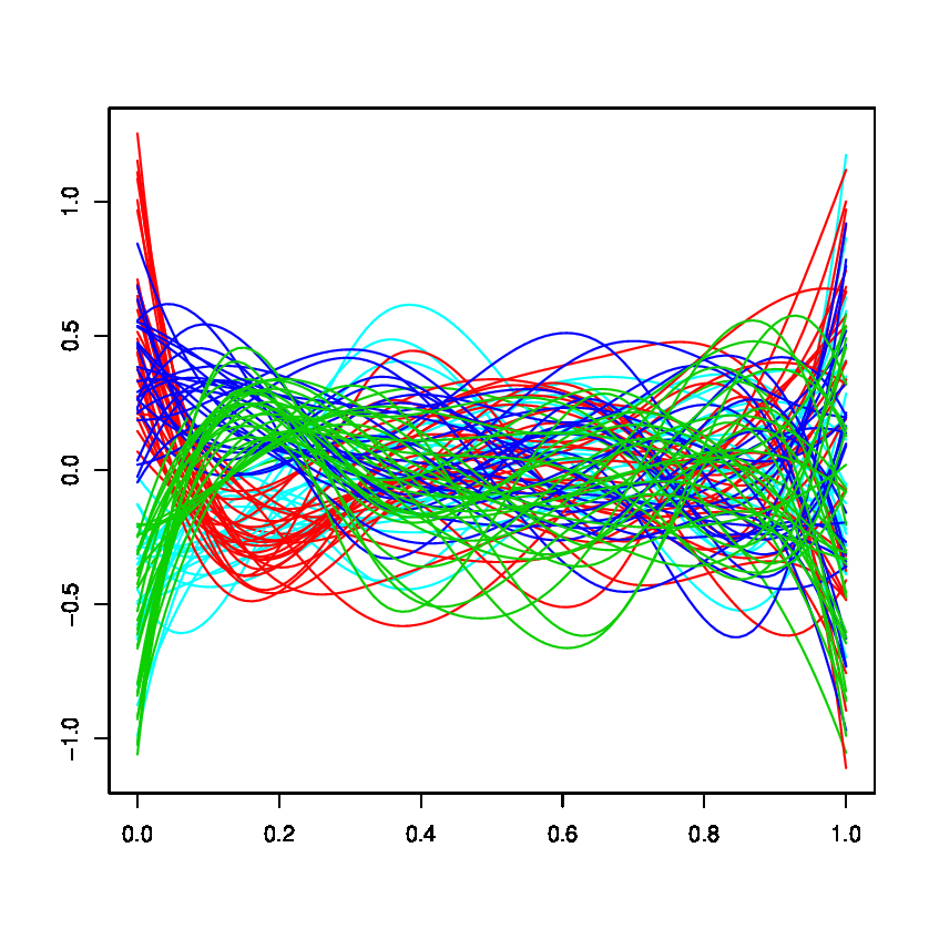
Let $\boldsymbol{\phi}$ be the fourth-order B-spline basis functions with eight knots, and let $\mathbf{\Phi}$ be a $T\times M$ matrix whose $tm$th element is $\phi_{m}(t)$. In this simulation study, we consider 100 sampling points $\boldsymbol{t}=(1,\dots,100)$ and 10 basis functions. Then, an artificial data matrix that includes discretized functional data was calculated as $\mathbf{X}=\mathbf{G}_{H}\mathbf{H}^{-\frac{1}{2}}\mathbf{\Phi}^{\prime}$. Note that before calculating $\mathbf{X}$, the columns of $\mathbf{G}_{H}$ were standardized. The artificial data selected are shown in Figure 4.

In this simulation analysis, four factors were manipulated in the experiment: (1) the number of objects ($N$), (2) the expected proportion of overlap (PO) between clusters in the correct subspace, (3) the ranks of the coefficient matrices $\mathbf{G}_{1}$ and $\mathbf{G}_{2}$, and (4) the number of variables which have no information about the true cluster structure (the number of non-informative variables, NN). The number of objects was varied from $100$ to $500$ in steps of $200$. The PO was defined as the proportion of shared density between clusters, as proposed by Steinley and Henson (2005). The PO was set at four levels: 0.0001, 0.05, 0.10, and 0.15. To offer an impression of the effect of the manipulation of the PO, an example of $\mathbf{F}$ for 200 objects in four clusters is depicted in Figure 5, for each of the different levels of the PO.

We consider four cases with the combination of ranks of $\mathbf{G}_{1}$ and $\mathbf{G}_{2}$; for each coefficient matrix, we consider two cases, full rank (FR) or rank deficient (RD). The rank of $\mathbf{G}_{1}$ was controlled by the number of columns $M_{1}$, which was set at 2 for the FR case and 5 for the RD case. For a FR case of $\mathbf{G}_{2}$, the elements of $\mathbf{G}_{2}$ were independently drawn from a standard normal distribution $N(0,1)$, while for a RD case, $\mathbf{G}_{2}$ was calculated as $\mathbf{G}_{2}=\mathbf{E}\mathbf{A}_{2}^{\prime}$, where $\mathbf{E}$ is an $N\times(M_{2}-2)$ matrix and $\mathbf{A}$ is an $M_{2}\times(M_{2}-2)$ matrix. The size $M_{2}-2$ implies that the rank of $\mathbf{G}_{2}$ is two lower than that of the FR case. The elements of $\mathbf{E}$ and $\mathbf{A}_{2}$ were independently drawn from $N(0,1)$ and $\mathbf{A}_{2}$ was subsequently orthonormalized. When $\mathbf{G}_{1}$ and $\mathbf{G}_{2}$ are FR, FFKM works well but FPCK does not. On the other hand, when $\mathbf{G}_{1}$ is RD and $\mathbf{G}_{2}$ is FR, FPCK works well but FFKM does not. Furthermore, it can be inferred that both FFKM and FPCK are effected negatively by the rank deficiency of $\mathbf{G}_{2}$. A non-informative variable $\mathbf{Z}$ was also generated through the basis function expansion $\mathbf{Z}=\mathbf{G}_{H}^{*}\mathbf{H}^{-\frac{1}{2}}\mathbf{\Phi}^{\prime}$ in which elements of a coefficient matrix $\mathbf{G}_{H}^{*}$ were independently drawn from $N(0,1)$ and standardized to have a same variance with the informative data $\mathbf{X}$. In this study, the number of non-informative variables was set at three levels: 0, 1, and 2. The experimental design was fully crossed, with $50$ replicates per cell, yielding $3\times 4\times 4\times 3\times 50=7200$ simulated data sets.

The cluster membership recovery was assessed by the adjusted Rand index (ARI; Hubert and Arabie, 1985). The ARI has the maximal value of $1$ in the case of a perfect recovery of the underlying clustering structure, and a value of $0$ in the case where the true membership $U$ and estimated membership $\hat{U}$ coincide no more than would be expected by chance. When the PO is high, the $k$-means clustering in the true subspace defined by the true $\mathbf{A}_{1}$ does not work. Thus, in order to calculate the ARI, the $k$-means clustering with 100 random starts was conducted with the true $\mathbf{F}$, and then the estimated cluster structure was considered to be the true cluster structure.

In addition, to evaluate recovery of the subspace, the root-mean-squared error criterion was calculated:

where $\boldsymbol{v}_{l}^{*}$ is the true weight function, $\hat{\boldsymbol{v}}_{l}$ is the estimate of $\boldsymbol{v}_{l}^{*}$, and $\|\cdot\|_{P}$ denotes the norm in $\mathscr{L}^{P}$ with $P$ functional variables (see, Appendix A). In this case, the true weight function is defined as $\boldsymbol{v}_{l}^{*}=(v_{l1}^{*},\dots,v_{lP}^{*})$ with $v_{l1}^{*}=\mathbf{\Phi}\mathbf{H}^{-\frac{1}{2}}\boldsymbol{a}_{Hl}$ where $\boldsymbol{a}_{Hl}$ is the $l$th column of $\mathbf{A}_{H}=(\mathbf{A}_{1}^{\prime},\mathbf{O}_{L\times M_{2}})^{\prime}$, and for $p>1$, $v_{lp}^{*}$ is equal to a zero function. Note that the FFKM model has indeterminacy of rotation of weight functions, as is also true of the FPCK model (Yamamoto, 2012). Thus, the RMSE criterion for each of the methods was calculated after the Procrustes rotation, so that the true weight function $\boldsymbol{v}_{l}^{*}$ was considered to be the target.

The FFKM and FPCK methods need initial values for the parameters in the first step of the algorithms. In our limited experience, FFKM is rather sensitive to local optima so that it needs many initial values. Thus, in this simulation, we used 1000 random initial values for FFKM and 100 random initial values for FPCK. For two-step FFKM, a selection of the number $R$ of components in the first step is needed. In this simulation, $R$ was determined in view of cumulative percentage of the total variation (Jolliffe, 2002) in which a selected cut-off provided 90% cumulative variation.

Boxplots of the ARIs obtained by the four methods are shown in Figure 6, 7, 8, and 9 which are results for the cases of (FR, FR), (RD, FR), (FR, RD), and (RD, RD), respectively, corresponding to the ranks of ($\mathbf{G}_{1},\mathbf{G}_{2}$). The modified boxplot (Hubert and Vandervieren, 2008) was used for the asymmetry of the distributions of ARIs and RMSEs. In these figures, boxplots of four methods for each sample size are arranged by the proportion of overlap (PO) and the number of non-informative variables (NN). As can be inferred from Figure 6, when both $\mathbf{G}_{1}$ and $\mathbf{G}_{2}$ were FR, under all conditions, FFKM and two-step FFKM showed the best result, or at least a result comparable to those of the other two methods. It can be seen that ARIs became worse with an increase in PO and NN, while the indices improved with an increase in the sample size. FPCK also worked well only under the easiest condition where PO was small, $N$ was large, and there was no non-informative variable. This result shows that the FPCK method provided a poor result if the contributing part $\mathbf{G}_{1}$ to the cluster structure was FR. We also see that tandem analysis did not work well, regardless of the chosen values of PO, NN, and $N$.

When $\mathbf{G}_{1}$ was RD and $\mathbf{G}_{2}$ was FR (Figure 7), we can see that FPCK showed the best result under all values of PO and NN, while FFKM did not. The two-step FFKM method provided better results when $\text{PO}=0.0001$ than when PO was large, and the ARI became worse with an increase in PO and NN. Since $\mathbf{G}_{2}$ was FR and all columns of $\mathbf{G}_{1}$ contributed to the cluster structure, the optimal subspace obtained from functional principal component analysis are coincident with that obtained from FPCK. This fact explains that tandem analysis worked as well as FPCK in this case.

When $\mathbf{G}_{1}$ was FR and $\mathbf{G}_{2}$ was RD (Figure 8), only two-step FFKM recovered the true cluster structure. It can be inferred that FFKM were effected negatively by the correlation of $\mathbf{G}_{2}$, while two-step FFKM improved the performance of FFKM to remove the negative effect of the cumbersome correlation as it had been expected.

When both $\mathbf{G}_{1}$ and $\mathbf{G}_{2}$ were RD (Figure 9), FPCK showed the best result, or at least a result comparable to those of other methods. Two-step FFKM also worked well under mild conditions in which both PO and NN were small. FFKM and tandem analysis did not recovered the cluster structure well because of the existence of substantial correlation of $\mathbf{G}_{2}$.

Boxplots of the RMSEs obtained by the four methods are shown in Figure 10, 11, 12, and 13 which are results for the cases of (FR, FR), (RD, FR), (FR, RD), and (RD, RD), respectively, corresponding to the ranks of ($\mathbf{G}_{1},\mathbf{G}_{2}$). From these figures, it can be seen that the results of RMSEs coincide with those of ARIs.

We used 1000 random starts for the FFKM method. However, even in the case of one of the easiest settings, where $\text{PO}=0.0001$ and $N=500$, only 93 initial starts attained the global optimal solution. In addition, more local optimal solutions seem to occur when the overlap is increased. Thus, in practice, it is necessary to check carefully whether the solution is a global optimal solution. If not, more initial random starts may be necessary.

References

- [1] [Arabie, P., Hubert, L., 1994.] Cluster analysis in marketting research. In: Bagozzi, R.P. (Ed.), Handbook of marketing research. Blackwell, Oxford.
- [2] [Besse, P.C., Ramsay, J.O., 1986.] Principal components analysis of sampled functions. Psychometorika 51 (2), 285–311.
- [3] [Boente, G., Fraiman, R., 2000.] Kernel-based functional principal components. Statistics & Probability Letters 48 (4), 335–345.
- [4] [Bouveyron, C., Jacques, J., 2011.] Model-based clustering of time series in group-specific functional subspaces. Advances in Data Analysis and Classification 5, 281–300.
- [5] [De Soete, G., Carroll, J.D., 1994.] K-means clustering in a low-dimensional Euclidean space. In: Diday, E., Lechevallier, Y., Schader, M., Bertrand, P., Burtschy, B. (Eds.), New approaches in classification and data analysis. Springer, Berlin, Heidelberg, pp. 212–219.
- [6] [DeSarbo, W.S., Jedidi, K., Cool, K., Schendel, D., 1990.] Simultaneous multidimensional unfolding and cluster analysis: An investigation of strategic groups. Marketing Letters 2 (2), 129–146.
- [7] [Dunford, N., Schwartz. J.T., 1988.] Linear operators, spectral theory, self adjoint operators in Hilbert space, part 2. Interscience, NewYork.
- [8] [Ferraty, F., Vieu, P., 2003.] Curves discrimination: a non parametric functional approach. Computational Statistics & Data Analysis 44, 161–173.
- [9] [Gattone, S.A., Rocci, R., 2012.] Clustering curves on a reduced subspace. Journal of Computational and Graphical Statistics 21 (2), 361–379.
- [10] [Green, P.J., Silverman, B.W., 1994.] Nonparametric regression and generalized linear models: a roughness penalty approach. Chapman and Hall, London.
- [11] [Hardy, A., 1996.] On the number of clusters. Computational Statistics & Data Analysis 23, 83–96.
- [12] [Hastie, T., Buja, A., Tibshirani, R., 1995.] Penalized discriminant analysis. The Annals of Statistics 23 (1), 73–102.
- [13] [Hubert, L., Arabie, P., 1985.] Comparing partitions. Journal of Classification 2, 193–218.
- [14] [Hubert, M., Vandervieren, E., 2008.] An adjusted boxplot for skewed distributions. Computational Statistics & Data Analysis 52, 5186–5201.
- [15] [Illian, J.B., Prosser. J.I., Baker, K.L., Rangel-Castro, J.I., 2009.] Functional principal component data analysis: A new method for analysing microbial community fingerprints. Journal of Microbiological Methods 79 (1), 89–95.
- [16] [Jolliffe, I.T., 2002.] Principal component analysis, 2nd Edition. Springer, New York.
- [17] [Kneip, A., 1994.] Nonparametric estimation of common regressors for similar curve data. The Annals of Statistics 22 (3), 1386–1427.
- [18] [Lloyd, S., 1982.] Least squares quantization in pem. IEEE Transactions on Information Theory 28 (2), 128–137.
- [19] [Milligan, G.W., Cooper, M.C., 1985.] An examination of procedures for determining the number of clusters in a data set. Psychometrika 50 (2), 159–179.
- [20] [Ocaña, F.A., Aguilera, A.M., Valderrama, M.J., 1982.] Functional principal components analysis by choice of norm. Journal of Multivariate Analysis 71, 262–276.
- [21] [Pezzulli, S.D., Silverman, B.W., 1993.] Some properties of smoothed principal components analysis for functional data. Computational Statistics 8 (1), 1–16.
- [22] [Ramsay, J.O., Silverman, B.W., 2005.] Functional Data Analysis, 2nd Edition. Springer, New York.
- [23] [Reiss, T.P., Ogden, T., 2007.] Functional principal component regression and functional prtial least squares. Journal of the American Statistical Association 102 (479), 984–996.
- [24] [Rice, J.A., Silverman, B.W., 1991.] Estimating the mean and covariance structure nonparametrically when the data are curves. Journal of the Royal Statistical Society: Series B 53 (1), 233–243.
- [25] [Silverman, B.W., 1996.] Smoothed functional principal components analysis by choice of norm. The Annals of Statistics 24 (1), 1–24.
- [26] [Steinley, D., Henson, R., 2005.] Oclus: an analytic method for generating clusters with known overlap. Journal of classification 22, 221–250.
- [27] [Suyundykov, R., Puechmorel, S., Ferre, L., 2010.] Multivariate functional data clusterization by PCA in Sobolev space using wavelets. Hyper Articles en Ligne :inria-00494702.
- [28] [ten Berge, J.M.F., 1993.] Least squares optimization in multivariate analysis. DSWO Press, Leiden University, Leiden.
- [29] [Timmerman, M.E., Ceulemans, E., Kiers, H.A.L., Vichi, M., 2010.] Factorial and reduced k-means reconsidered. Computational Statistics & Data Analysis 54, 1858–1871.
- [30] [Vichi, M., Kiers H.A.L., 2001.] Factorial k-means analysis for two-way data. Computational Statistics & Data Analysis 37 (1), 49–64.
- [31] [Vidal, R., 2011.] Subspace clustering. Signal Processing Magazine, IEEE 28, 52–68.
- [32] [Wahba, G., 1990.] Spline models for observational data. Society for Industrial and Applied Mathematics, Philadelphia.
- [33] [Wang, J., 2010.] Consistent selection of the number of clusters via crossvalidation. Biometrika 97 (4), 893–904.
- [34] [Yamamoto, M., 2012.] Clustering of functional data in a low-dimensional subspace. Advances in Data Analysis and Classification 6, 219–247.