Shared kernel Bayesian screening

In modern biomedical research, it is common to screen for differences between groups in many variables. These variables are often measured using the same technology and are not well characterized using a simple parametric distribution. As an example we consider DNA methylation arrays. Methylation is an epigenetic phenomenon that can affect transcription and occurs at genomic locations where a cytosine nucleotide is followed by a guanine nucleotide, called a CpG site. High-throughput microarrays are commonly used to measure methylation levels for thousands of CpG sites genome-wide. Measurements are typically collected from a tissue that contains several distinct cell types, and at a given CpG site each cell type is typically either methylated or unmethylated (Reinius et al., 2012). Arrays therefore give continuous measurements for discrete methylation states and the resulting values are between $0$, no methylation, and $1$, fully methylated. Figure 1 shows the distribution of methylation measurements over individuals for three CpG sites using data from the Cancer Genome Atlas Network (2012). Multi-modality and skewness are common; kernel mixtures are useful for modeling such complexity.

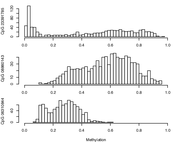
Methylation variables share several distributional features such as common support, common modes and common patterns of skewness. The use of kernels that are shared across variables thus not only reduces computational burden but can also improve performance. It is also natural to share kernels across groups, with the interpretation that two groups arise from the same discrete process but in potentially different proportions.

We introduce a simple, computationally efficient, and theoretically supported Bayesian approach for screening using shared kernels across groups and, if appropriate, across variables. The population distribution for each variable is approximated using a mixture of kernels $\{F_{k}\}_{k=1}^{K}$. For two groups $0$ and $1$, we test whether the groups have different kernel weights. Specifically, for group distributions $F_{m}^{(0)}$ and $F_{m}^{(1)}$ at variable $m$, $F_{m}^{(0)}=\sum_{k=1}^{K}\pi_{mk}^{(0)}F_{k}$ and $F_{m}^{(1)}=\sum_{k=1}^{K}\pi_{mk}^{(1)}F_{k}$, the competing hypotheses are

In practice $F_{1},...,F_{K}$ and a shared Dirichlet prior distribution for the weights $\Pi_{m}^{(0)},\Pi_{m}^{(1)}$ are estimated empirically. A simple and tractable Gibbs sampling procedure is then used to estimate the posterior probability of $H_{0m}$ for each variable.

While methylation array data provide excellent motivation, our framework addresses the general statistical problem of testing for equality between two groups that are drawn from the same strata but in potentially different proportions. We argue that the method may also be useful for applications that do not have such a clear interpretation, and this is supported with theoretical results in Section 4.

The multi-modality of methylation measurements is widely recognized (Laird, 2010) but often not accounted for in practice. The two-sample t-test is most commonly used to identify sites of differential expression in case-control studies (Bock, 2012). Alternative testing approaches are rank-based or discretize the data based on arbitrary thresholds (Chen et al., 2011; Qiu & Zhang, 2012). Other statistical models have been proposed to identify CpG sites that are hypomethylated, hypermethylated or undifferentiated with respect to normal cells (Khalili et al., 2007; Akalin et al., 2012). The focus on differential methylation levels between groups may miss other important differences between group distributions; for example, certain genomic regions have been shown to exhibit more variability in methylation, and thus epigenetic instability, among cancer cells than among normal cells (Hansen et al., 2011).

Although our model involves finite mixtures, it is intended to be robust to parametric assumptions and so is comparable to nonparametric methods. There is a literature on nonparametric Bayes testing of equivalence in distribution between groups. Dunson & Peddada (2008) use a dependent Dirichlet process to test for equality against stochastically ordered alternatives. They use an interval test based on total variation distance, and the framework is easily extended to unordered alternatives. Pennell & Dunson (2008) also use a Dirichlet process model for multiple groups and an interval test. Ma & Wong (2011) and Holmes et al. (2015) use Polya tree priors to test for exact equality. Existing nonparametric Bayes tests do not exploit shared features among variables, in the form of shared kernels or otherwise.

If kernel memberships are known, our testing framework (1) is equivalent to a test for association with a $2\times K$ contingency table. For this there are standard frequentist methods such as Fisher’s exact test and Pearson’s chi-square test, and established Bayesian methods (Good & Crook, 1987; Albert, 1997). In our context the component memberships are unknown and are inferred probabilistically. Xu et al. (2010) addressed this as part of a series of comparisons for Bayesian mixture distributions between groups. They compare marginal likelihoods for models with and without assuming constant weights between groups. Our focus is instead on screening settings in which there are many variables, and it is important to borrow information while adjusting for multiple testing. Shared kernels facilitate borrowing of information and computational scaling, and in our implementation a shared prior for the probability of equality at each variable induces a multiplicity adjustment with favorable properties (Scott & Berger, 2006; Muller et al., 2007; Scott & Berger, 2010).

Below we describe the general model for shared kernel Bayesian screening. Details that are specific to our implementation for methylation array data, including estimation techniques that facilitate posterior computation in high-dimensions, are given in Section 5.

First we describe a shared kernel mixture model, to lay the groundwork for the two-group screening model in Section 2.2. Given data $x_{mn}$ for $M$ variables ($m=1,\ldots,M$) and $N$ subjects ($n=1,\ldots,N$), the shared kernel model assumes that observations $x_{mn}$ are realized from one of $K$ component distributions $F_{1},\ldots,F_{K}$. Typically $x_{mn}$ is a continuous and unidimensional observation, but we present the model in sufficient generality to allow for more complex data structures. We assume that$F_{1},\ldots,F_{K}$ have corresponding likelihoods from the same parametric family $f(\cdot,\theta_{k})$.

Let $c_{mn}\in\{1,\ldots,K\}$ represent the component generating $x_{mn}$, and $\pi_{mk}=\operatorname{pr}(c_{mn}=k)$ be the probability that an arbitrary subject belongs to component $k$ in variable $m$. The generative model is $x_{mn}\sim F_{k}\text{ with probability }\pi_{mk}$. Under a Bayesian framework one puts a prior distribution on $\{\Pi_{m}=(\pi_{m1},\ldots,\pi_{mK})\}_{m=1}^{M}$ and, if they are unspecified, the kernels $F_{1},\ldots,F_{K}$. It is natural to use a Dirichlet conjugate prior for $\Pi_{m}$, characterized by a $K$-dimensional parameter $\alpha$ of positive real numbers. Small values of $\alpha$, with $\alpha_{k}\leq 1$, will favor small values for a subset of the $\pi_{mk}$ values. Thus, some kernels may have negligible impact for a given variable.

We extend the shared kernel model above to allow for two sample groups: $X^{(0)}$ with data $x_{mn}^{(0)}$ for $N_{0}$ subjects ($n=1,\ldots,N_{0}$; $m=1,\ldots,M$), and $X^{(1)}$ with data $x_{mn}^{(1)}$ for $N_{1}$ subjects ($n=1,\ldots,N_{1}$; $m=1,\ldots,M$). Observations for all $M$ variables are realized from a common set of kernels $F_{1},\ldots,F_{K}$, but the two groups have potentially different weights $\{\Pi_{m}^{(0)}\}_{m=1}^{M}$ and $\{\Pi_{m}^{(1)}\}_{m=1}^{M}$.

The weights $\Pi_{m}^{(0)}$ and $\Pi_{m}^{(1)}$ each have prior distribution Dir($\alpha$), whether they are identical or not. Let $H_{0m}$ be the event that the mixing weights are the same for both groups: $\Pi_{m}^{(0)}=\Pi_{m}^{(1)}$. Under $H_{1m}$, $\Pi_{m}^{(0)}$ and $\Pi_{m}^{(1)}$ are considered independent realizations from Dir($\alpha$). Let $F_{m}^{(0)}$ be the distribution for group $0$ and let $F_{m}^{(1)}$ be the distribution for group $1$. We consider a dummy variable $\mathbbm{1}(H_{0m})\sim\text{Bernoulli}\{\operatorname{pr}(H_{0m})\}$ and independent realizations $\tilde{\Pi}_{mk},\tilde{\Pi}_{mk}^{(0)},\tilde{\Pi}_{mk}^{(1)}\sim\text{Dir}(\alpha)$ to give the joint distribution for groups $i=0,1$:

As $\operatorname{pr}(H_{0m})\rightarrow 1$, $F_{m}^{(0)}$ and $F_{m}^{(1)}$ share the same mixing weights, and as $\operatorname{pr}(H_{0m})\rightarrow 0$ the weights are independent.

Let $\vec{n}_{m}^{(0)}=(n_{m1}^{(0)},\ldots,n_{mK}^{(0)})$ give the number of subjects in group $0$ that belong to each kernel $k$ in variable $m$, and define $\vec{n}_{m}^{(1)}$ similarly for group $1$. Then, $\vec{n}_{m}=\vec{n}_{m}^{(0)}+\vec{n}_{m}^{(1)}$ gives the total number of subjects allocated to each component. Under $H_{0m}$, the distribution for the component memberships $C_{m}^{(0)}$ and $C_{m}^{(1)}$ is

where $\Gamma$ is the gamma function and $\beta$ is the multivariate beta function $\beta(\alpha)=\prod_{k=1}^{K}\Gamma(\alpha_{k})/\Gamma(\sum_{k=1}^{K}\alpha_{k})$. Similarly, under $H_{1m}$,

Let the shared prior probability of no difference be $P_{0}=\operatorname{pr}(H_{0m})$ for all $m$. The posterior probability of $H_{0m}$ given $C_{m}^{(0)}$ and $C_{m}^{(1)}$ is

But in practice the kernel memberships are unknown, and the kernels may be unknown as well. There is no analogous closed form that accounts for uncertainty in $(C_{m}^{(0)},C_{m}^{(1)})$ and direct computation is usually infeasible. We instead employ a Gibbs sampling procedure that uses (2) to approximate the full posterior distribution. Under multiple related tests, $M>1$, we infer $P_{0}$ using a Be$(a,b)$ prior, where by default $a=b=1$. The mean of the realized values of $\operatorname{pr}(H_{0m}\mid C_{m}^{(0)},C_{m}^{(1)})$ over the sampling iterations is used to estimate the posterior probability of $H_{0m}$ for each variable.

While this article focuses on the two-group case, extensions to multiple groups are straightforward. A natural approach is to define a prior to cluster the groups. For example, we could use a Dirichlet process as in Gopalan & Berry (1998), but instead of clustering group means we would be clustering group distributions. Each cluster would then have a separate weight vector drawn from a Dirichlet distribution.

The above approach is presented in the context of shared kernels for high-dimensional screening, large $M$. The framework is also useful in the simple case $M=1$, and is particularly well motivated when two groups have the same strata but in potentially different proportions. The theoretical results presented in Sections 3 and  4 are not specific to high-dimensional screening, and we drop the variable subscript $m$ for simplicity.

We illustrate our approach on a methylation array dataset for $N=597$ breast cancer samples and $M=21,986$ CpG sites. These data are publicly available from the TCGA Data Portal (Cancer Genome Atlas Network, 2012). We focus on testing for a difference between tumours that are identified as basal-like ($N_{0}=112$) against those that are not ($N_{1}=485$) at each site. Basal-like samples have a relatively poor clinical prognosis and a distinct gene expression profile, but the role of DNA methylation in this distinction has not been well characterized.

For scalability and to borrow information across sites, we apply a two-stage procedure. First, a set of dictionary kernels are estimated. Specifically, for $k=1,\ldots,K$, $f_{k}$ is the density of a normal distribution with mean $\mu_{k}$ and precision $\tau_{k}$ truncated to fall within the interval $[0,1]$. We use a normal-gamma prior for $\mu_{k}$ and $\tau_{k}$. For computational reasons we estimate the posterior for $f_{1},\ldots,f_{K}$ from a sub-sample of $500$ sites, for an effective sample size of $597\times 500=298,500$ observations. We employ a Gibbs sampler and update the common Dirichlet prior parameter $\alpha$ at each iteration using maximum likelihood estimation (Ronning, 1989). Alternatively one could use a hyperprior for $\alpha$, but this complicates posterior estimation and probably has little influence on posterior estimates as the effective sample size is very large. Similarly, we find there is little uncertainty in the posterior mean and variance for each kernel; we can ignore the error in estimating these densities and fix them in the second stage.

The number of kernels $K=9$ is chosen by cross validation based on the mean log-likelihood for held-out observations. Estimates for the dictionary densities $f_{1},\ldots,f_{9}$ are shown in Figure 2; to address the label switching problem, we order the kernels by their means and then average over Gibbs samples. For fixed $f_{1},\ldots,f_{9}$, we compute the posterior for the two-group model at each CpG site using a simple and efficient Gibbs sampler and a uniform hyperprior for $P_{0}$. We calculate the component likelihoods $f_{k}(x_{mn})$ for all sites $m$, samples $n$, and components $k$ in advance, which greatly reduces the computational burden.

We run Gibbs sampling for the two-group model for all $21,986$ CpG sites, with $5000$ iterations, after a $1000$ iteration burn-in. The draws mix well and converge quickly; mixing is considerably improved by fixing the dictionary densities.

The global prior probability of no difference, inferred using a uniform hyperprior, was $\hat{P}_{0}=0.821$. The estimated posterior probabilities $\operatorname{pr}(H_{0m}\mid X)$ are shown in Figure 3. These have a U-shaped distribution, with 91% of values falling below $0.05$ or above $0.95$. Many values are close to 1, suggesting that these methylation sites play no role in the distinction between basal and non-basal tumours.

Figure 4 shows the sample distributions and mixture density fits for basal and non-basal tumours at four CpG sites. These four sites were selected to show a range of estimated differences between the distributions for basal and non-basal tumours. In general, the estimated mixture densities appear to fit the data well. Some CpG sites with posterior probabilities $\operatorname{pr}(H_{0m}\mid X)$ that are very small have dramatically different distributions between the two groups. For the majority of CpG sites, the estimated distributions for the two groups are nearly identical. The method naturally borrows strength across groups to estimate a common density when $\operatorname{pr}(H_{0m}\mid X)\rightarrow 1$, and estimates the two densities separately when $\operatorname{pr}(H_{0m}\mid X)\rightarrow 0$.

We investigated the potential relevance of differentially distributed CpG sites by considering the expression of the gene at their genomic location. DNA methylation is thought to primarily inhibit transcription and therefore repress gene expression. Of 2117 CpG sites with $\operatorname{pr}(H_{0m}\mid X)<0.01$, 1256 have a significant negative association with gene expression using Spearman’s rank correlation, p-value $<0.01$. For these cases methylation gives a potential mechanistic explanation for well-known differences in gene transcription levels between basal and non-basal tumours. In particular, these include five genes from the well-known PAM50 gene signature for breast cancer subtyping (Parker et al., 2009): MYBL2, EGFR, MIA, SFRP1 and MLPH. A supplemental spreadsheet gives the posterior probability $\operatorname{pr}(H_{0m}\mid X)$ and corresponding gene expression statistics for all CpG sites.

References

- Akalin et al. (2012) Akalin, A., Kormaksson, M., Li, S., Garrett-Bakelman, F. E., Figueroa, M. E., Melnick, A., Mason, C. E. et al. (2012). methylKit: a comprehensive R package for the analysis of genome-wide DNA methylation profiles. Genome Biology 13, R87.
- Albert (1997) Albert, J. H. (1997). Bayesian testing and estimation of association in a two-way contingency table. J. Am. Statist. Assoc. 92, 685–693.
- Bock (2012) Bock, C. (2012). Analysing and interpreting DNA methylation data. Nat. Rev. Genet. 13, 705–719.
- Cancer Genome Atlas Network (2012) Cancer Genome Atlas Network (2012). Comprehensive molecular portraits of human breast tumours. Nature 490, 61–70.
- Chen et al. (2011) Chen, M., Zaas, A., Wood, C., Ginsberg, G., Lucas, J., Dunson, D. & Carin, L. (2011). Predicting viral infection from high-dimensional biomarker trajectories. J. Am. Statist. Assoc. 106, 1259–1279.
- Dunson & Peddada (2008) Dunson, D. B. & Peddada, S. D. (2008). Bayesian nonparametric inference on stochastic ordering. Biometrika 95, 859–874.
- Good & Crook (1987) Good, I. & Crook, J. (1987). The robustness and sensitivity of the mixed-Dirichlet Bayesian test for “independence” in contingency tables. Ann. Statist. 15, 670–693.
- Gopalan & Berry (1998) Gopalan, R. & Berry, D. A. (1998). Bayesian multiple comparisons using Dirichlet process priors. J. Am. Statist. Assoc. 93, 1130–1139.
- Hansen et al. (2011) Hansen, K. D., Timp, W., Bravo, H. C., Sabunciyan, S., Langmead, B., McDonald, O. G., Wen, B., Wu, H., Liu, Y., Diep, D. et al. (2011). Increased methylation variation in epigenetic domains across cancer types. Nat. Genet. 43, 768–775.
- Holmes et al. (2015) Holmes, C. C., Caron, F., Griffin, J. E. & Stephens, D. A. (2015). Two-sample Bayesian nonparametric hypothesis testing. Bayesian Anal. 10, 297–320.
- Johnson & Rossell (2010) Johnson, V. E. & Rossell, D. (2010). On the use of non-local prior densities in bayesian hypothesis tests. J. R. Statist. Soc. B 72, 143–170.
- Kass & Raftery (1995) Kass, R. E. & Raftery, A. E. (1995). Bayes factors. J. Am. Statist. Assoc. 90, 773–795.
- Khalili et al. (2007) Khalili, A., Potter, D., Yan, P., Li, L., Gray, J., Huang, T. & Lin, S. (2007). Gamma-normal-gamma mixture model for detecting differentially methylated loci in three breast cancer cell lines. Cancer Informatics 3, 43.
- Kleijn & van der Vaart (2006) Kleijn, B. J. & van der Vaart, A. W. (2006). Misspecification in infinite-dimensional Bayesian statistics. Ann. Statist. 34, 837–877.
- Laird (2010) Laird, P. W. (2010). Principles and challenges of genome-wide DNA methylation analysis. Nat. Rev. Genet. 11, 191–203.
- Ma & Wong (2011) Ma, L. & Wong, W. H. (2011). Coupling optional Pólya trees and the two sample problem. J. Am. Statist. Assoc. 106, 1553–1565.
- Muller et al. (2007) Muller, P., Parmigiani, G. & Rice, K. (2007). FDR and Bayesian multiple comparisons rules. In Bayesian Statistics 8, J. M. Bernardo, R. Bayarri, J. O. Berger, A. P. Dawid, D. Heckerman, A. F. M. Smith & M. West, eds. Oxford: Oxford University Press, pp. 349–370.
- Parker et al. (2009) Parker, J. S., Mullins, M., Cheang, M. C., Leung, S., Voduc, D., Vickery, T., Davies, S., Fauron, C., He, X., Hu, Z. et al. (2009). Supervised risk predictor of breast cancer based on intrinsic subtypes. Journal of Clinical Oncology 27, 1160–1167.
- Pennell & Dunson (2008) Pennell, M. L. & Dunson, D. B. (2008). Nonparametric Bayes testing of changes in a response distribution with an ordinal predictor. Biometrics 64, 413–423.
- Qiu & Zhang (2012) Qiu, P. & Zhang, L. (2012). Identification of markers associated with global changes in DNA methylation regulation in cancers. BMC Bioinformatics 13, S7.
- Reinius et al. (2012) Reinius, L. E., Acevedo, N., Joerink, M., Pershagen, G., Dahlén, S.-E., Greco, D., Söderhäll, C., Scheynius, A. & Kere, J. (2012). Differential dna methylation in purified human blood cells: implications for cell lineage and studies on disease susceptibility. PloS one 7, e41361.
- Ronning (1989) Ronning, G. (1989). Maximum likelihood estimation of Dirichlet distributions. J. Stat. Comput. Simul. 32, 215–221.
- Scholz & Stephens (1987) Scholz, F. & Stephens, M. (1987). K-sample Anderson–Darling tests. J. Am. Statist. Assoc. 82, 918–924.
- Scott & Berger (2006) Scott, J. G. & Berger, J. O. (2006). An exploration of aspects of Bayesian multiple testing. J. Statist. Plann. Inference 136, 2144–2162.
- Scott & Berger (2010) Scott, J. G. & Berger, J. O. (2010). Bayes and empirical-Bayes multiplicity adjustment in the variable-selection problem. Ann. Statist. 38, 2587–2619.
- Teicher (1963) Teicher, H. (1963). Identifiability of finite mixtures. Ann. Math. Statist. 34, 1265–1269.
- Walker (2004) Walker, S. G. (2004). Modern Bayesian asymptotics. Statistical Science 19, 111–117.
- Xu et al. (2010) Xu, L., Hanson, T., Bedrick, E. J. & Restrepo, C. (2010). Hypothesis tests on mixture model components with applications in ecology and agriculture. J. Agric. Biol. Environ. Stat. 15, 308–326.
- Yakowitz et al. (1968) Yakowitz, S. J., Spragins, J. D. et al. (1968). On the identifiability of finite mixtures. Ann. Math. Statist. 39, 209–214.