跳到论文正文
W Papers独立论文阅读器 arXiv:1311.0283 论文正文 计算阅读时间 · 0%
引用这篇论文根据当前论文元数据生成,正式投稿前建议核对。


License: arXiv.org perpetual non-exclusive license
arXiv:1311.0283v1 [hep-ph] 01 Nov 2013
\contribID

xy

\desyproc

DESY-PROC-2013-03 \acronymHQ2013

Top Quark Production

Nikolaos Kidonakis
Kennesaw State University
   Physics #1202    1000 Chastain Rd    Kennesaw    GA 30144    USA
Abstract

I discuss top quark production in hadronic collisions. I present the soft-gluon resummation formalism and its derivation from factorization and renormalization-group evolution, and two-loop calculations of soft anomalous dimensions in the eikonal approximation. I discuss the contributions of next-to-next-to-leading order (NNLO) soft-gluon corrections to the total cross sections and top-quark transverse momentum and rapidity distributions for top-antitop pair production, and for single-top production in the tt and ss channels and in association with a WW boson or a charged Higgs boson.

1 Introduction

The top quark is the heaviest elementary particle known to date. It was discovered in proton-antiproton collisions at the Fermilab Tevatron in 1995 in top-antitop pair production events by the CDF and D0 Collaborations [1, 2]. The uniqueness of the top quark is not only due to its heavy mass, which makes it important for Higgs physics, but also due to the fact that it is the only quark that decays before it can hadronize. Top-antitop pair and single-top production have by now been fully established at both the Tevatron and the LHC and are in good agreement with theoretical expectations, as we will see later in detail.

In these lectures I discuss top quark production in hadron colliders, paying particular attention to higher-order corrections from soft-gluon resummation. I begin with a discussion of higher-order soft-gluon corrections, factorization, renormalization-group evolution (RGE), resummation, and next-to-next-to-leading order (NNLO) expansions.

I continue with one- and two-loop eikonal diagrams, calculations of the massive cusp anomalous dimension, and presentation of the the two-loop soft anomalous dimension matrices for top-pair production.

I then provide results for t​t¯t{\bar{t}} production, including the total t​t¯t{\bar{t}} cross sections at the LHC and the Tevatron, the top-quark transverse momentum, pTp_{T}, distributions, and the top-quark rapidity distributions. Finally, I discuss single-top production, in particular tt-channel and ss-channel production, and t​W−tW^{-} and t​H−tH^{-} production, and present total cross sections and top-quark pTp_{T} distributions.

2 Higher-order soft-gluon corrections

QCD corrections are significant for hard-scattering cross-sections, and in particular for top-pair and single-top production. The complete next-to-leading order (NLO) corrections were calculated for t​t¯t{\bar{t}} production in [3, 4] and for single-top production in [5].

Soft-gluon corrections, i.e. perturbative corrections from the emission of soft (low-energy) gluons, originate from incomplete cancellations of infrared divergences between virtual diagrams and real diagrams with soft gluons.

The soft-gluon terms are of the form [lnk⁡(s4/mt2)s4]+\left[\frac{\ln^{k}(s_{4}/m_{t}^{2})}{s_{4}}\right]_{+} where k≤2​n−1k\leq 2n-1 for the nnth-order perturbative corrections, and s4s_{4} is the kinematical distance from partonic threshold. The leading logarithms (LL) are those with the highest power, 2​n−12n-1; the next-to-leading logarithms (NLL) have a power of one less; the next-to-next-to-leading logarithms (NNLL) have a power of two less, etc. The importance of soft-gluon corrections is because they are dominant near threshold. It is possible to resum (i.e. exponentiate) these corrections to all orders in perturbative QCD. This resummation follows from factorization of the cross section and RGE of its factors. The resummation of the leading logarithms requires universal terms describing the emission of collinear and soft gluons that only depend on the identity of the incoming and outgoing partons, i.e. the details of the hard process are irrelevant. However, at NLL accuracy [6] and beyond it is necessary to involve the process-dependent color exchange in the hard-scattering process and to perform the corresponding loop calculations in the eikonal approximation.

In addition to these soft-gluon logarithmic terms there also arise terms of purely collinear origin, of the form 1mt2​lnk⁡(s4/mt2)\frac{1}{m_{t}^{2}}\ln^{k}(s_{4}/m_{t}^{2}), but we will not dicuss these kind of terms in this paper.

Complete results are now available at NNLL accuracy, which requires the calculation of two-loop soft anomalous dimensions. For a review of resummation for top quark production see Ref. [7]. Approximate next-to-next-to-leading order (NNLO) double-differential cross sections and even next-to-next-to-next-to-leading order (NNNLO) corrections have been derived from the expansion of the resummed results [8].

2.1 Factorization, RGE, and Resummation

We consider hadronic processes of the form

h1​(ph1)+h2​(ph2)→t⁡(p)+X\displaystyle h_{1}(p_{h_{1}})+h_{2}(p_{h_{2}})\rightarrow t(p)+X

where h1h_{1}, h2h_{2}, are colliding hadrons (protons at the LHC; protons and antiprotons at the Tevatron) and tt denotes the observed top quark with XX all additional final-state particles. The underlying partonic processes are of the form

f1​(p1)+f2​(p2)→t⁡(p)+X\displaystyle f_{1}(p_{1})\,+\,f_{2}\,(p_{2})\rightarrow t(p)\,+\,X

where f1f_{1} and f2f_{2} represent partons (quarks or gluons). We define s=(p1+p2)2s=(p_{1}+p_{2})^{2}, t=(p1−p)2t=(p_{1}-p)^{2}, u=(p2−p)2u=(p_{2}-p)^{2}. Also s4=s+t+u−∑m2s_{4}=s+t+u-\sum m^{2}, where the sum is over the squared masses of all particles in the process. Thus, s4s_{4} measures distance from partonic threshold, where there is no energy for additional radiation, but the top quark may have arbitrary momentum and is not restricted to be produced at rest (thus partonic threshold is more general than absolute, or production, threshold where the top quark is produced at rest). At partonic threshold s4=0s_{4}=0.

The factorization for the (in general differential) cross section is expressed by the formula

d​σh1​h2→t​X\displaystyle d\sigma_{h_{1}h_{2}\rightarrow tX} =\displaystyle= ∑f1,f2∫d​x1​d​x2​ϕf1/h1​(x1,μF)​ϕf2/h2​(x2,μF)​σ^f1​f2→t​X​(s4,s,t,u,μF,μR)\displaystyle\sum_{f_{1},f_{2}}\;\int dx_{1}\,dx_{2}\,\phi_{f_{1}/h_{1}}(x_{1},\mu_{F})\,\phi_{f_{2}/h_{2}}(x_{2},\mu_{F})\,{\hat{\sigma}}_{f_{1}f_{2}\rightarrow tX}(s_{4},s,t,u,\mu_{F},\mu_{R})

where ϕ\phi are parton distribution functions with x1x_{1} and x2x_{2} the momentum fractions of partons f1f_{1} and f2f_{2} in hadrons h1h_{1} and h2h_{2} respectively, μF\mu_{F} is the factorization scale and μR\mu_{R} is the renormalization scale. We factorize the initial-state collinear divergences into the parton distribution functions, ϕ\phi. Soft-gluon corrections appear in the partonic hard-scattering cross section, σ^f1​f2→t​X{\hat{\sigma}}_{f_{1}f_{2}\rightarrow tX}, as plus distributions of logarithmic terms, defined through their integral with parton distribution functions

∫0s4​m​a​xd​s4​ϕ​(s4)​[lnk⁡(s4/mt2)s4]+\displaystyle\int_{0}^{s_{4\,max}}ds_{4}\,\phi(s_{4})\left[\frac{\ln^{k}(s_{4}/m_{t}^{2})}{s_{4}}\right]_{+} ≡\displaystyle\equiv ∫0s4​m​a​xd​s4​lnk⁡(s4/mt2)s4​[ϕ⁡(s4)−ϕ⁡(0)]\displaystyle\int_{0}^{s_{4\,max}}ds_{4}\frac{\ln^{k}(s_{4}/m_{t}^{2})}{s_{4}}[\phi(s_{4})-\phi(0)]
+1k+1​lnk+1⁡(s4​m​a​xmt2)​ϕ​(0).\displaystyle{}+\frac{1}{k+1}\ln^{k+1}\left(\frac{s_{4\,max}}{m_{t}^{2}}\right)\phi(0)\,.

Resummation follows from the factorization properties of the cross section, performed in moment space. We define moments of the partonic cross section by σ^(N)=∫(ds4/s)e−Ns4/sσ^(s4){\hat{\sigma}}(N)=\int(ds_{4}/s)\;e^{-Ns_{4}/s}{\hat{\sigma}}(s_{4}). The logarithms of s4s_{4} give rise to logarithms of NN in moment space, and we will show that the logarithms of NN appearing in σ^​(N){\hat{\sigma}}(N) exponentiate.

We then write a factorized expression for the infrared-regularized (with ϵ=4−n\epsilon=4-n) parton-parton scattering cross section, σf1​f2→t​X​(N,ϵ)\sigma_{f_{1}f_{2}\rightarrow tX}(N,\epsilon), in moment space

σf1​f2→t​X​(N,ϵ)=ϕf1/f1​(N,μF,ϵ)​ϕf2/f2​(N,μF,ϵ)​σ^f1​f2→t​X​(N,μF,μR)\displaystyle\sigma_{f_{1}f_{2}\rightarrow tX}(N,\epsilon)=\phi_{f_{1}/f_{1}}(N,\mu_{F},\epsilon)\;\phi_{f_{2}/f_{2}}(N,\mu_{F},\epsilon)\;{\hat{\sigma}}_{f_{1}f_{2}\rightarrow tX}(N,\mu_{F},\mu_{R})

which factorizes similarly to the hadronic cross section, with ϕ⁡(N)=∫01d​x​xN−1​ϕ​(x)\phi(N)=\int_{0}^{1}dx\;x^{N-1}\phi(x).

Refer to caption     Refer to caption

Figure 1: Factorization of the partonic cross section for t​t¯t{\bar{t}} production: (a) The functions involved in the partonic process; (b) the soft-gluon function SS.

The partonic function σ^f1​f2→t​X{\hat{\sigma}}_{f_{1}f_{2}\rightarrow tX} still has sensitivity to soft-gluon dynamics via its NN dependence. We then refactorize the cross section [6] in terms of modified parton distributions ψ\psi, defined in the partonic center-of-mass frame at fixed energy, as

σf1​f2→t​X​(N,ϵ)\displaystyle\sigma_{f_{1}f_{2}\rightarrow tX}(N,\epsilon) =\displaystyle= ψf1/f1​(N,μF,ϵ)​ψf2/f2​(N,μF,ϵ)\displaystyle\psi_{f_{1}/f_{1}}\left(N,\mu_{F},\epsilon\right)\;\psi_{f_{2}/f_{2}}\left(N,\mu_{F},\epsilon\right)
×HI​Lf1​f2→t​X​(αs​(μR))​SL​If1​f2→t​X​(mtN​μF,αs​(μR))​∏jJj​(N,μF,ϵ).\displaystyle\times\;H_{IL}^{f_{1}f_{2}\rightarrow tX}\left(\alpha_{s}(\mu_{R})\right)\;S_{LI}^{f_{1}f_{2}\rightarrow tX}\left(\frac{m_{t}}{N\mu_{F}},\alpha_{s}(\mu_{R})\right)\;\prod_{j}J_{j}\left(N,\mu_{F},\epsilon\right)\,.

This factorization is shown for the case of top-antitop pair production in Fig. 1(a).

The HI​Lf1​f2→t​XH_{IL}^{f_{1}f_{2}\rightarrow tX} are NN-independent hard-scattering terms which involve contributions from the amplitude of the process and the complex conjugate of the amplitude, in the form HI​L=hL∗​hIH_{IL}=h_{L}^{*}\,h_{I}. Also, SL​If1​f2→t​XS_{LI}^{f_{1}f_{2}\rightarrow tX} is the soft gluon function for non-collinear soft-gluon emission; it represents the coupling of soft gluons to the partons in the scattering with color tensors cIc_{I}, cLc_{L} (see Fig. 1(b)). Both HI​LH_{IL} and SL​IS_{LI} are process dependent and they are matrices in the space of color exchanges in the partonic scattering. JJ are jet functions describing universal soft and collinear emission from any outgoing massless partons.

Comparing the two previous equations, we find

σ^f1​f2→t​X​(N,μF,μR)\displaystyle{\hat{\sigma}}_{f_{1}f_{2}\rightarrow tX}(N,\mu_{F},\mu_{R}) =\displaystyle= ψf1/f1​(N,μF,ϵ)​ψf2/f2​(N,μF,ϵ)ϕf1/f1​(N,μF,ϵ)​ϕf2/f2​(N,μF,ϵ)\displaystyle\frac{\psi_{f_{1}/f_{1}}(N,\mu_{F},\epsilon)\,\psi_{f_{2}/f_{2}}(N,\mu_{F},\epsilon)}{\phi_{f_{1}/f_{1}}(N,\mu_{F},\epsilon)\,\phi_{f_{2}/f_{2}}(N,\mu_{F},\epsilon)}
×HI​Lf1​f2→t​X​(αs​(μR))​SL​If1​f2→t​X​(mtN​μF,αs​(μR))​∏jJj​(N,μF,ϵ).\displaystyle\times\;H_{IL}^{f_{1}f_{2}\rightarrow tX}\left(\alpha_{s}(\mu_{R})\right)\,S_{LI}^{f_{1}f_{2}\rightarrow tX}\left(\frac{m_{t}}{N\mu_{F}},\alpha_{s}(\mu_{R})\right)\prod_{j}J_{j}\left(N,\mu_{F},\epsilon\right)\,.

All the factors in the above equation are gauge and factorization scale dependent. The requirement that the product of these factors be independent of the gauge and the factorization scale results in the exponentiation of logarithms of NN in the ratios ψf1/f1/ϕf1/f1\psi_{f_{1}/f_{1}}/\phi_{f_{1}/f_{1}} and ψf2/f2/ϕf2/f2\psi_{f_{2}/f_{2}}/\phi_{f_{2}/f_{2}}, in the soft-gluon matrix SL​IS_{LI}, and in the functions JjJ_{j}.

The soft matrix SL​IS_{LI} requires renormalization as a composite operator; its NN-dependence can then be resummed via RGE [6]. The product HI​L​SL​IH_{IL}S_{LI} however needs no overall renormalization, because the UV divergences of HI​LH_{IL} balance those of SL​IS_{LI}. We have

HI​Lb\displaystyle H^{b}_{IL} =\displaystyle= (∏i=1,2Zi−1)​(ZS−1)I​A​HA​B​[(ZS†)−1]B​L\displaystyle\left(\prod_{i=1,2}Z_{i}^{-1}\right)\;\left(Z_{S}^{-1}\right)_{IA}H_{AB}\left[\left(Z_{S}^{\dagger}\right)^{-1}\right]_{BL}
SL​Ib\displaystyle S^{b}_{LI} =\displaystyle= (ZS†)L​C​SC​D​ZS,D​I\displaystyle(Z_{S}^{\dagger})_{LC}S_{CD}Z_{S,DI}

where HbH^{b} and SbS^{b} are the unrenormalized quantities, ZiZ_{i} are the renormalization constants of the incoming partonic fields, and ZSZ_{S} is a matrix of renormalization constants, which describe the renormalization of the soft function, including the wave functions for outgoing heavy-quark eikonal lines.

Thus SL​IS_{LI} satisfies the renormalization group equation

(μ​∂∂μ+β⁡(gs)​∂∂gs)​SL​I=−(ΓS†)L​C​SC​I−SL​D​(ΓS)D​I\displaystyle\left(\mu\frac{\partial}{\partial\mu}+\beta(g_{s})\frac{\partial}{\partial g_{s}}\right)\,S_{LI}=-(\Gamma^{\dagger}_{S})_{LC}S_{CI}-S_{LD}(\Gamma_{S})_{DI}

where gs2=4​π​αsg_{s}^{2}=4\pi\alpha_{s} and β\beta is the QCD beta function

β(αs)≡12​αsd​αsd​ln⁡μ=μdlngs/dμ=−β0αs/(4π)−β1αs2/(4π)2+⋯,\displaystyle\beta(\alpha_{s})\equiv\frac{1}{2\alpha_{s}}\frac{d\alpha_{s}}{d\ln\mu}=\mu\,d\ln g_{s}/d\mu=-\beta_{0}\alpha_{s}/(4\pi)-\beta_{1}\alpha_{s}^{2}/(4\pi)^{2}+\cdots\,,

with β0=(11​CA−2​nf)/3\beta_{0}=(11C_{A}-2n_{f})/3 and β1=34​CA2/3−2​nf​(CF+5​CA/3)\beta_{1}=34C_{A}^{2}/3-2n_{f}(C_{F}+5C_{A}/3). Here CF=(Nc2−1)/(2​Nc)C_{F}=(N_{c}^{2}-1)/(2N_{c}) and CA=NcC_{A}=N_{c}, with Nc=3N_{c}=3 the number of colors, and nfn_{f} is the number of light quark flavors (nf=5n_{f}=5 for top production).

ΓS\Gamma_{S} is the soft anomalous dimension matrix that controls the evolution of the soft function SS. In dimensional regularization ZSZ_{S} has 1/ϵ1/\epsilon poles, and ΓS\Gamma_{S} is given at one loop in terms of the residue of ZSZ_{S} by

ΓS(1−l​o​o​p)​(gs)=−gs2​∂∂gs​Resϵ→0​ZS​(gs,ϵ).\displaystyle\Gamma_{S}^{(1-loop)}(g_{s})=-\frac{g_{s}}{2}\frac{\partial}{\partial g_{s}}{\rm Res}_{\epsilon\rightarrow 0}Z_{S}(g_{s},\epsilon)\,.

The soft anomalous dimension ΓS\Gamma_{S} is a matrix in color space and a function of the kinematical invariants ss, tt, uu. The process-dependent matrices ΓS\Gamma_{S} have been calculated at one loop for all 2→22\rightarrow 2 partonic processes. For the q​q¯→t​t¯q{\bar{q}}\rightarrow t{\bar{t}} process, ΓS\Gamma_{S} is a 2×22\times 2 matrix [6]. For the g​g→t​t¯gg\rightarrow t{\bar{t}} process, ΓS\Gamma_{S} is a 3×33\times 3 matrix [6]. Explicit expressions at one and two loops will be provided in Section 4.

The resummed cross section in moment space, denoted as σ^f1​f2→t​Xr​e​s​(N){\hat{\sigma}}_{f_{1}f_{2}\rightarrow tX}^{res}(N) below, follows from the RGE of all the functions in the factorized cross section, and can be written in the form:

σ^f1​f2→t​Xr​e​s​(N)\displaystyle{\hat{\sigma}}_{f_{1}f_{2}\rightarrow tX}^{res}(N) =\displaystyle= exp⁡[∑i=1,2Ei​(Ni)]​exp⁡[∑jEj′​(N′)]​exp​[∑i=1,22​∫μFsd​μμ​γi/i​(N~i,αs​(μ))]\displaystyle\exp\left[\sum_{i=1,2}E_{i}(N_{i})\right]\,\exp\left[\sum_{j}E^{\prime}_{j}(N^{\prime})\right]\;\exp\left[\sum_{i=1,2}2\int_{\mu_{F}}^{\sqrt{s}}\frac{d\mu}{\mu}\;\gamma_{i/i}\left({\tilde{N}}_{i},\alpha_{s}(\mu)\right)\right]\;
×tr{Hf1​f2→t​X(αs(s))exp[∫ss/N~′d​μμΓS†f1​f2→t​X(αs(μ))]\displaystyle\times\,{\rm tr}\left\{H^{f_{1}f_{2}\rightarrow tX}\left(\alpha_{s}(\sqrt{s})\right)\exp\left[\int_{\sqrt{s}}^{{\sqrt{s}}/{\tilde{N}^{\prime}}}\frac{d\mu}{\mu}\;\Gamma_{S}^{\dagger\,f_{1}f_{2}\rightarrow tX}\left(\alpha_{s}(\mu)\right)\right]\right.
×Sf1​f2→t​X(αs(sN~′))exp[∫ss/N~′d​μμΓSf1​f2→t​X(αs(μ))]}\displaystyle\left.\times\,S^{f_{1}f_{2}\rightarrow tX}\left(\alpha_{s}\left(\frac{\sqrt{s}}{\tilde{N}^{\prime}}\right)\right)\;\exp\left[\int_{\sqrt{s}}^{{\sqrt{s}}/{\tilde{N}^{\prime}}}\frac{d\mu}{\mu}\;\Gamma_{S}^{f_{1}f_{2}\rightarrow tX}\left(\alpha_{s}(\mu)\right)\right]\right\}

where the trace is taken of the product of the color-space matrices HH, SS, and exponents of ΓS\Gamma_{S} and its Hermitian conjugate, ΓS†\Gamma_{S}^{\dagger}.

The collinear and soft radiation from incoming partons is resummed via the first exponential with

Ei​(Ni)\displaystyle E_{i}(N_{i}) =\displaystyle= ∫01d​z​zNi−1−11−z​{∫1(1−z)2d​λλ​Ai​(αs​(λ​s))+Di​[αs​((1−z)2​s)]}\displaystyle\int^{1}_{0}dz\frac{z^{N_{i}-1}-1}{1-z}\;\left\{\int_{1}^{(1-z)^{2}}\frac{d\lambda}{\lambda}A_{i}\left(\alpha_{s}(\lambda s)\right)+D_{i}\left[\alpha_{s}((1-z)^{2}s)\right]\right\}

(for purely collinear corrections, replace zN−1−11−z\frac{z^{N-1}-1}{1-z}\; by −zN−1\;-z^{N-1} in the above expression). Here N1=N⁡(mt2−u)/mt2N_{1}=N(m_{t}^{2}-u)/m_{t}^{2} and N2=N⁡(mt2−t)/mt2N_{2}=N(m_{t}^{2}-t)/m_{t}^{2}. The term AiA_{i} has the perturbative expansion Ai=αsπ​Ai(1)+(αsπ)2​Ai(2)+⋯A_{i}=\frac{\alpha_{s}}{\pi}A_{i}^{(1)}+\left(\frac{\alpha_{s}}{\pi}\right)^{2}A_{i}^{(2)}+\cdots where Ai(1)=CiA_{i}^{(1)}=C_{i} [9] with Ci=CFC_{i}=C_{F} for a quark or antiquark and Ci=CAC_{i}=C_{A} for a gluon, while Ai(2)=Ci​K/2A_{i}^{(2)}=C_{i}K/2 [10] with K=CA​(67/18−ζ2)−5​nf/9K=C_{A}\;(67/18-\zeta_{2})-5n_{f}/9 [11]. Here and below we use ζ2=π2/6\zeta_{2}=\pi^{2}/6, ζ3=1.2020569⋯\zeta_{3}=1.2020569\cdots, and ζ4=π4/90\zeta_{4}=\pi^{4}/90. Also Di=(αs/π)​Di(1)+(αs/π)2​Di(2)+⋯D_{i}=(\alpha_{s}/\pi)D_{i}^{(1)}+(\alpha_{s}/\pi)^{2}D_{i}^{(2)}+\cdots with Di(1)=0D_{i}^{(1)}=0 in Feynman gauge (Di(1)=−CiD_{i}^{(1)}=-C_{i} in axial gauge). In Feynman gauge the two-loop result is [12]

Di(2)=Ci​CA​(−10154+116​ζ2+74​ζ3)+Ci​nf​(727−ζ23).\displaystyle D_{i}^{(2)}=C_{i}C_{A}\left(-\frac{101}{54}+\frac{11}{6}\zeta_{2}+\frac{7}{4}\zeta_{3}\right)+C_{i}n_{f}\left(\frac{7}{27}-\frac{\zeta_{2}}{3}\right)\,.

The collinear and soft radiation from outgoing massless quarks and gluons is resummed via the second exponential

Ej′​(N′)\displaystyle E_{j}^{\prime}(N^{\prime}) =\displaystyle= ∫01dzzN′−1−11−z{∫(1−z)21−zd​λλAj(αs(λs))+Bj[αs((1−z)s)]\displaystyle\int^{1}_{0}dz\frac{z^{N^{\prime}-1}-1}{1-z}\left\{\int^{1-z}_{(1-z)^{2}}\frac{d\lambda}{\lambda}A_{j}\left(\alpha_{s}\left(\lambda s\right)\right)+B_{j}\left[\alpha_{s}((1-z)s)\right]\right.
+Dj[αs((1−z)2s)]}\displaystyle\hskip 79.66771pt\left.+D_{j}\left[\alpha_{s}((1-z)^{2}s)\right]\right\}

where N′=N​s/mt2N^{\prime}=N\,s/m_{t}^{2}. Note that this exponent is not needed in t​t¯t{\bar{t}} production but it is used in single-top production. The term BjB_{j} has the perturbative expansion Bj=(αs/π)​Bj(1)+(αs/π)2​Bj(2)+⋯B_{j}=(\alpha_{s}/\pi)B_{j}^{(1)}+(\alpha_{s}/\pi)^{2}B_{j}^{(2)}+\cdots with Bq(1)=−3CF/4B_{q}^{(1)}=-3C_{F}/4 for a quark or antiquark, and Bg(1)=−β0/4B_{g}^{(1)}=-\beta_{0}/4 for a gluon [9, 10]. Also (c.f. [12, 13])

Bq(2)=CF2​(−332+34​ζ2−32​ζ3)+CF​CA​(−5732−1112​ζ2+34​ζ3)+nf​CF​(516+ζ26),\displaystyle B_{q}^{(2)}=C_{F}^{2}\left(-\frac{3}{32}+\frac{3}{4}\zeta_{2}-\frac{3}{2}\zeta_{3}\right)+C_{F}C_{A}\left(-\frac{57}{32}-\frac{11}{12}\zeta_{2}+\frac{3}{4}\zeta_{3}\right)+n_{f}C_{F}\left(\frac{5}{16}+\frac{\zeta_{2}}{6}\right)\,,
Bg(2)=CA2​(−1025432−34​ζ3)+79108​CA​nf+CF​nf8−5108​nf2.\displaystyle B_{g}^{(2)}=C_{A}^{2}\left(-\frac{1025}{432}-\frac{3}{4}\zeta_{3}\right)+\frac{79}{108}C_{A}\,n_{f}+C_{F}\frac{n_{f}}{8}-\frac{5}{108}n_{f}^{2}\,.

The factorization scale dependence in the third exponential is controlled by the moment-space anomalous dimension of the MS¯{\overline{\rm MS}} density ϕi/i\phi_{i/i}, which is γi/i=−Ai​ln⁡N~i+γi\gamma_{i/i}=-A_{i}\ln{\tilde{N}}_{i}+\gamma_{i} [14, 15], where N~i=Ni​eγE{\tilde{N}}_{i}=N_{i}e^{\gamma_{E}} with γE\gamma_{E} the Euler constant. The parton anomalous dimensions γi\gamma_{i} have the perturbative expansion

γi=(αs/π)​γi(1)+(αs/π)2​γi(2)+⋯\displaystyle\gamma_{i}=(\alpha_{s}/\pi)\gamma_{i}^{(1)}+(\alpha_{s}/\pi)^{2}\gamma_{i}^{(2)}+\cdots

with γq(1)=3​CF/4\gamma_{q}^{(1)}=3C_{F}/4, γg(1)=β0/4\gamma_{g}^{(1)}=\beta_{0}/4,

γq(2)=CF2​(332−34​ζ2+32​ζ3)+CF​CA​(1796+1112​ζ2−34​ζ3)+nf​CF​(−148−ζ26)\displaystyle\gamma_{q}^{(2)}=C_{F}^{2}\left(\frac{3}{32}-\frac{3}{4}\zeta_{2}+\frac{3}{2}\zeta_{3}\right)+C_{F}C_{A}\left(\frac{17}{96}+\frac{11}{12}\zeta_{2}-\frac{3}{4}\zeta_{3}\right)+n_{f}C_{F}\left(-\frac{1}{48}-\frac{\zeta_{2}}{6}\right)

and

γg(2)=CA2​(23+34​ζ3)−nf​(CF8+CA6).\displaystyle\gamma_{g}^{(2)}=C_{A}^{2}\left(\frac{2}{3}+\frac{3}{4}\zeta_{3}\right)-n_{f}\left(\frac{C_{F}}{8}+\frac{C_{A}}{6}\right)\,.

The relation between αs\alpha_{s} at two different scales, μ\mu and μR\mu_{R}, is

αs​(μ)\displaystyle\alpha_{s}(\mu) =\displaystyle= αs(μR)[1−β04​παs(μR)ln(μ2μR2)+β0216​π2αs2(μR)ln2(μ2μR2)−β116​π2αs2(μR)ln(μ2μR2)\displaystyle\alpha_{s}(\mu_{R})\left[1-\frac{\beta_{0}}{4\pi}\alpha_{s}(\mu_{R})\ln\left(\frac{{\mu}^{2}}{\mu_{R}^{2}}\right)+\frac{\beta_{0}^{2}}{16\pi^{2}}\alpha_{s}^{2}(\mu_{R})\ln^{2}\left(\frac{{\mu}^{2}}{\mu_{R}^{2}}\right)-\frac{\beta_{1}}{16\pi^{2}}\alpha_{s}^{2}(\mu_{R})\ln\left(\frac{{\mu}^{2}}{\mu_{R}^{2}}\right)\right.
+⋯].\displaystyle\hskip 56.9055pt\left.+\cdots\right]\,.

We write the perturbative expansions for the hard-scattering function HH and the soft-gluon function SS as

H=αsdαs​H(0)+αsdαs+1π​H(1)+αsdαs+2π2​H(2)+⋯\displaystyle H=\alpha_{s}^{d_{\alpha_{s}}}H^{(0)}+\frac{\alpha_{s}^{d_{\alpha_{s}}+1}}{\pi}H^{(1)}+\frac{\alpha_{s}^{d_{\alpha_{s}}+2}}{\pi^{2}}H^{(2)}+\cdots

and

S=S(0)+αsπ​S(1)+αs2π2​S(2)+⋯\displaystyle S=S^{(0)}+\frac{\alpha_{s}}{\pi}S^{(1)}+\frac{\alpha_{s}^{2}}{\pi^{2}}S^{(2)}+\cdots

respectively, where dαsd_{\alpha_{s}} denotes the power of αs\alpha_{s} in the Born cross section. At lowest order, the trace of the product of the hard matrices HH and soft matrices SS gives the Born cross section for each partonic process, σB=αsdαs​tr​[H(0)​S(0)]\sigma^{B}=\alpha_{s}^{d_{\alpha_{s}}}{\rm tr}[H^{(0)}S^{(0)}].

Noncollinear soft gluon emission is controlled by the soft anomalous dimension ΓS\Gamma_{S}, which has the perturbative expansion

ΓS=αsπ​ΓS(1)+αs2π2​ΓS(2)+⋯\displaystyle\Gamma_{S}=\frac{\alpha_{s}}{\pi}\Gamma_{S}^{(1)}+\frac{\alpha_{s}^{2}}{\pi^{2}}\Gamma_{S}^{(2)}+\cdots

We determine ΓS\Gamma_{S} from the coefficients of ultraviolet poles in dimensionally regularized eikonal diagrams. The determination of ΓS(1)\Gamma_{S}^{(1)} is needed for NLL resummation and it requires one-loop calculations in the eikonal approximation; ΓS(2)\Gamma_{S}^{(2)} is needed for NNLL resummation and requires two-loop calculations.

Complete two-loop results are now known for the soft anomalous dimensions for many processes, and in these lectures I will review results for:

∙\bullet the soft (cusp) anomalous dimension for e+​e−→t​t¯e^{+}e^{-}\rightarrow t{\bar{t}}

∙\bullet t​t¯t{\bar{t}} hadroproduction

∙\bullet tt-channel single top production

∙\bullet ss-channel single top production

∙\bullet b​g→t​W−bg\rightarrow tW^{-} and b​g→t​H−bg\rightarrow tH^{-}

2.2 NLO and NNLO expansions

The resummed cross section suffers from infrared divergences that need a prescription to be dealt with. However, the numerical results depend on the prescription, and differences between prescriptions are typically larger than corrections beyond NNLO. Thus, an alternative and preferred procedure is to expand the resummed cross section to a fixed order in the perturbative expansion, thus avoiding arbitrary prescription dependences. Thus the resummed cross section is used as a generator of higher-order soft-gluon corrections, and here we present expansions to NNLO (for NNNLO see the second paper in [8]).

In the moment-space resummed cross section we are resumming lnk⁡N\ln^{k}N; we then expand to fixed order and invert back to momentum space to get the usual lnk⁡(s4/mt2)/s4\ln^{k}(s_{4}/m_{t}^{2})/s_{4} terms.

We will use the following notation for the logarithmic plus distributions,

𝒟k​(s4)≡[lnk⁡(s4/mt2)s4]+.\displaystyle{\cal D}_{k}(s_{4})\equiv\left[\frac{\ln^{k}(s_{4}/m_{t}^{2})}{s_{4}}\right]_{+}\,.

The NLO soft-gluon corrections from the expansion of the resummed cross section can be written as

σ^(1)=σB​αs​(μR)π​{c3​𝒟1​(s4)+c2​𝒟0​(s4)+c1​δ​(s4)}+αsdαs+1​(μR)π​[Ac​𝒟0​(s4)+T1c​δ​(s4)]\displaystyle{\hat{\sigma}}^{(1)}=\sigma^{B}\frac{\alpha_{s}(\mu_{R})}{\pi}\left\{c_{3}\,{\cal D}_{1}(s_{4})+c_{2}\,{\cal D}_{0}(s_{4})+c_{1}\,\delta(s_{4})\right\}+\frac{\alpha_{s}^{d_{\alpha_{s}}+1}(\mu_{R})}{\pi}\left[A^{c}\,{\cal D}_{0}(s_{4})+T_{1}^{c}\,\delta(s_{4})\right]

where we have separated contributions into a part proportional to the Born term, i.e. the leading-order (LO) term, σB\sigma^{B}, and a part that is not (in general) proportional to it. The leading logarithmic coefficient is

c3=∑i2​Ai(1)−∑jAj(1),\displaystyle c_{3}=\sum_{i}2\,A_{i}^{(1)}-\sum_{j}A_{j}^{(1)}\,,

and is always multiplied by σB\sigma^{B}. The next-to-leading logarithmic terms are in general not all proportional to σB\sigma^{B} and are separated into two parts. The first part has coefficient c2c_{2} which is defined by c2=c2μ+T2c_{2}=c_{2}^{\mu}+T_{2}, with c2μ=−∑iAi(1)ln(μF2/mt2)c_{2}^{\mu}=-\sum_{i}A_{i}^{(1)}\ln(\mu_{F}^{2}/m_{t}^{2}) denoting the terms involving logarithms of the scale, and

T2=∑i[−2​Ai(1)​ln⁡(−timt2)+Di(1)−Ai(1)​ln⁡(mt2s)]+∑j[Bj(1)+Dj(1)−Aj(1)​ln⁡(mt2s)].\displaystyle T_{2}=\sum_{i}\left[-2\,A_{i}^{(1)}\,\ln\left(\frac{-t_{i}}{m_{t}^{2}}\right)+D_{i}^{(1)}-A_{i}^{(1)}\ln\left(\frac{m_{t}^{2}}{s}\right)\right]+\sum_{j}\left[B_{j}^{(1)}+D_{j}^{(1)}-A_{j}^{(1)}\,\ln\left(\frac{m_{t}^{2}}{s}\right)\right]\,.

The part not in general proportional to σB\sigma^{B} is defined by

Ac=tr(H(0)ΓS(1)†S(0)+H(0)S(0)ΓS(1)).\displaystyle A^{c}={\rm tr}\left(H^{(0)}\Gamma_{S}^{(1)\,\dagger}S^{(0)}+H^{(0)}S^{(0)}\Gamma_{S}^{(1)}\right)\,.

The terms proportional to δ⁡(s4)\delta(s_{4}) include virtual corrections which cannot be determined from resummation as well as some terms that involve logarithms of the scales μF\mu_{F} and μR\mu_{R} and which can be calculated from the expansion of the resummed cross section. We write c1=c1μ+T1c_{1}=c_{1}^{\mu}+T_{1} with c1μc_{1}^{\mu} denoting the terms involving logarithms of the scale

c1μ=∑i[Ai(1)​ln⁡(−timt2)−γi(1)]​ln⁡(μF2mt2)+dαs​β04​ln⁡(μR2mt2).\displaystyle c_{1}^{\mu}=\sum_{i}\left[A_{i}^{(1)}\,\ln\left(\frac{-t_{i}}{m_{t}^{2}}\right)-\gamma_{i}^{(1)}\right]\ln\left(\frac{\mu_{F}^{2}}{m_{t}^{2}}\right)+d_{\alpha_{s}}\frac{\beta_{0}}{4}\ln\left(\frac{\mu_{R}^{2}}{m_{t}^{2}}\right)\,.

However T1T_{1} as well as T1cT_{1}^{c} can only be found from a complete NLO calculation.

The NNLO soft-gluon corrections from the expansion of the resummed cross section are then

σ^(2)\displaystyle{\hat{\sigma}}^{(2)} =\displaystyle= σBαs2​(μR)π2{12c32𝒟3(s4)+[32c3c2−β04c3+∑jβ08Aj(1)]𝒟2(s4)\displaystyle\sigma^{B}\frac{\alpha_{s}^{2}(\mu_{R})}{\pi^{2}}\left\{\frac{1}{2}c_{3}^{2}\,{\cal D}_{3}(s_{4})+\left[\frac{3}{2}c_{3}c_{2}-\frac{\beta_{0}}{4}c_{3}+\sum_{j}\frac{\beta_{0}}{8}A_{j}^{(1)}\right]{\cal D}_{2}(s_{4})\right.
+[c3​c1+c22−ζ2​c32−β02​T2+β04​c3​ln⁡(μR2mt2)+∑i2​Ai(2)−∑jAj(2)+∑jβ04​Bj(1)]​𝒟1​(s4)\displaystyle\hskip-28.45274pt{}+\left[c_{3}c_{1}+c_{2}^{2}-\zeta_{2}c_{3}^{2}-\frac{\beta_{0}}{2}T_{2}+\frac{\beta_{0}}{4}c_{3}\ln\left(\frac{\mu_{R}^{2}}{m_{t}^{2}}\right)+\sum_{i}2A_{i}^{(2)}-\sum_{j}A_{j}^{(2)}+\sum_{j}\frac{\beta_{0}}{4}B_{j}^{(1)}\right]{\cal D}_{1}(s_{4})
+[c2c1−ζ2c3c2+ζ3c32+β04c2ln(μR2s)−∑iβ02Ai(1)ln2(−timt2)\displaystyle\hskip-28.45274pt{}+\left[c_{2}c_{1}-\zeta_{2}c_{3}c_{2}+\zeta_{3}c_{3}^{2}+\frac{\beta_{0}}{4}c_{2}\ln\left(\frac{\mu_{R}^{2}}{s}\right)\right.-\sum_{i}\frac{\beta_{0}}{2}A_{i}^{(1)}\ln^{2}\left(\frac{-t_{i}}{m_{t}^{2}}\right)
+∑i[(−2Ai(2)+β02Di(1))ln(−timt2)+Di(2)+β08Ai(1)ln2(μF2s)−Ai(2)ln(μF2s)]\displaystyle\hskip-14.22636pt{}+\sum_{i}[\left(-2A_{i}^{(2)}+\frac{\beta_{0}}{2}D_{i}^{(1)}\right)\ln\left(\frac{-t_{i}}{m_{t}^{2}}\right)+D_{i}^{(2)}+\frac{\beta_{0}}{8}A_{i}^{(1)}\ln^{2}\left(\frac{\mu_{F}^{2}}{s}\right)-A_{i}^{(2)}\ln\left(\frac{\mu_{F}^{2}}{s}\right)]
+∑j[Bj(2)+Dj(2)−(Aj(2)+β04(Bj(1)+2Dj(1)))ln(mt2s)\displaystyle\hskip-14.22636pt{}+\sum_{j}[B_{j}^{(2)}+D_{j}^{(2)}-\left(A_{j}^{(2)}+\frac{\beta_{0}}{4}(B_{j}^{(1)}+2D_{j}^{(1)})\right)\ln\left(\frac{m_{t}^{2}}{s}\right)
+3​β08Aj(1)ln2(mt2s)]]𝒟0(s4)}\displaystyle\hskip 14.22636pt\left.\left.{}+\frac{3\beta_{0}}{8}A_{j}^{(1)}\ln^{2}\left(\frac{m_{t}^{2}}{s}\right)]\right]{\cal D}_{0}(s_{4})\right\}
+αsdαs+2​(μR)π2{32c3Ac𝒟2(s4)+[(2c2−β02)Ac+c3T1c+Fc]𝒟1(s4)\displaystyle\hskip-28.45274pt{}+\frac{\alpha_{s}^{d_{\alpha_{s}}+2}(\mu_{R})}{\pi^{2}}\left\{\frac{3}{2}c_{3}A^{c}\,{\cal D}_{2}(s_{4})+\left[\left(2c_{2}-\frac{\beta_{0}}{2}\right)A^{c}+c_{3}T_{1}^{c}+F^{c}\right]{\cal D}_{1}(s_{4})\right.
+[(c1−ζ2c3+β04ln(μR2s))Ac+c2T1c+Fcln(mt2s)+Gc]𝒟0(s4)}\displaystyle\hskip-14.22636pt\left.{}+\left[\left(c_{1}-\zeta_{2}c_{3}+\frac{\beta_{0}}{4}\ln\left(\frac{\mu_{R}^{2}}{s}\right)\right)A^{c}+c_{2}T_{1}^{c}+F^{c}\ln\left(\frac{m_{t}^{2}}{s}\right)+G^{c}\right]{\cal D}_{0}(s_{4})\right\}

where

Fc=tr[H(0)(ΓS(1)†)2S(0)+H(0)S(0)(ΓS(1))2+2H(0)ΓS(1)†S(0)ΓS(1)]F^{c}={\rm tr}\left[H^{(0)}\left(\Gamma_{S}^{(1)\,\dagger}\right)^{2}S^{(0)}+H^{(0)}S^{(0)}\left(\Gamma_{S}^{(1)}\right)^{2}+2H^{(0)}\Gamma_{S}^{(1)\,\dagger}S^{(0)}\Gamma_{S}^{(1)}\right]
Gc\displaystyle G^{c} =\displaystyle= tr[H(1)ΓS(1)†S(0)+H(1)S(0)ΓS(1)+H(0)ΓS(1)†S(1)+H(0)S(1)ΓS(1)\displaystyle{\rm tr}\left[H^{(1)}\Gamma_{S}^{(1)\,\dagger}S^{(0)}+H^{(1)}S^{(0)}\Gamma_{S}^{(1)}+H^{(0)}\Gamma_{S}^{(1)\,\dagger}S^{(1)}+H^{(0)}S^{(1)}\Gamma_{S}^{(1)}\right.
+H(0)ΓS(2)†S(0)+H(0)S(0)ΓS(2)]\displaystyle\quad\quad\left.{}+H^{(0)}\Gamma_{S}^{(2)\,\dagger}S^{(0)}+H^{(0)}S^{(0)}\Gamma_{S}^{(2)}\right]

and c3c_{3}, c2c_{2}, c1c_{1}, etc are from the NLO expansion. The two-loop universal quantities A(2)A^{(2)}, B(2)B^{(2)}, D(2)D^{(2)} were given previously. The two-loop process-dependent ΓS(2)\Gamma_{S}^{(2)} have been recently calculated for several processes, including top quark production in various channels.

In addition to the plus distributions, the factorization and renormalization scale dependent terms proportional to δ⁡(s4)\delta(s_{4}) at NNLO have also been calculated [8].

3 Two-loop calculations for the massive cusp anomalous dimension

Refer to caption

Figure 2: Elementary eikonal diagram for soft-gluon emission from an outgoing quark.

The Feynman rules for diagrams with soft gluon emission, see Fig. 2, simplify as

u¯​(p)​(−i​gs​TFc)​γμ​i(p/+k/+m)(p+k)2−m2+i​ϵ→u¯​(p)​gs​TFc​γμ​p/+m2​p⋅k+i​ϵ\displaystyle{\bar{u}}(p)\,(-ig_{s}T_{F}^{c})\,\gamma^{\mu}\frac{i(p\!\!/+k\!\!/+m)}{(p+k)^{2}-m^{2}+i\epsilon}\rightarrow{\bar{u}}(p)\,g_{s}T_{F}^{c}\,\gamma^{\mu}\frac{p\!\!/+m}{2p\cdot k+i\epsilon} =\displaystyle= u¯​(p)​gs​TFc​vμv⋅k+i​ϵ\displaystyle{\bar{u}}(p)\,g_{s}T_{F}^{c}\,\frac{v^{\mu}}{v\cdot k+i\epsilon}

with u¯{\bar{u}} a Dirac spinor, TFcT_{F}^{c} the generators of SU(3), and p∝vp\propto v, for example we may take pμ=s2​vμp^{\mu}=\sqrt{\frac{s}{2}}v^{\mu}, though other choices are possible. This is the eikonal approximation.

We perform the calculations here in momentum space and Feynman gauge. The first soft anomalous dimension that we consider is the massive cusp anomalous dimension, which is also the soft anomalous dimension for the process e+​e−→t​t¯e^{+}e^{-}\rightarrow t{\bar{t}} [16, 17].

3.1 One-loop cusp anomalous dimension

Refer to caption

Figure 3: One-loop eikonal diagrams for the cusp anomalous dimension.

The one-loop eikonal diagrams for the cusp anomalous dimension are shown in Fig. 3. The eikonal lines represent the top and the antitop quarks. The one-loop vertex correction is graph (a) and the one-loop top and antitop self-energy diagrams are the two graphs (b).

The one-loop soft anomalous dimension, ΓS(1)\Gamma_{S}^{(1)}, can be read off the coefficient of the ultraviolet (UV) pole of the one-loop diagrams. The calculation gives [16, 17]

ΓS(1)=CF​[−(1+β2)2​β​ln⁡(1−β1+β)−1]\displaystyle\Gamma_{S}^{(1)}=C_{F}\left[-\frac{(1+\beta^{2})}{2\beta}\ln\left(\frac{1-\beta}{1+\beta}\right)-1\right]

with β=1−4​mt2s\beta=\sqrt{1-\frac{4m_{t}^{2}}{s}}.

Refer to caption

Figure 4: One-loop vertex-correction diagram.

As an example of the calculation we provide some details for the vertex correction graph, i.e. diagram (a) of Fig. 3. This one-loop vertex correction is shown in more detail, and with momenta assignments, in Fig. 4. The integral corresponding to this diagram is

I1​a=gs2​∫dn​k(2​π)n​(−i)​gμ​νk2​viμvi⋅k​(−vjν)(−vj⋅k)\displaystyle I_{1a}=g_{s}^{2}\int\frac{d^{n}k}{(2\pi)^{n}}\frac{(-i)g^{\mu\nu}}{k^{2}}\frac{v_{i}^{\mu}}{v_{i}\cdot k}\,\frac{(-v_{j}^{\nu})}{(-v_{j}\cdot k)}

which has three factors. The first factor is the gluon propagator and the last two are the eikonal rules for the two lines. Using Feynman parameterization, this can be rewritten as

I1​a=−2igs2vi⋅vj(2​π)n∫01dx∫01−xdy∫dn​k[x​k2+y​vi⋅k+(1−x−y)​vj⋅k]3\displaystyle I_{1a}=-2ig_{s}^{2}\,\frac{v_{i}\cdot v_{j}}{(2\pi)^{n}}\int_{0}^{1}dx\int_{0}^{1-x}dy\int\frac{d^{n}k}{\left[xk^{2}+yv_{i}\cdot k+(1-x-y)v_{j}\cdot k\right]^{3}}

which, after the integration over kk, gives

I1​a\displaystyle I_{1a} =\displaystyle= gs2vi⋅vj 26−2​nπ−n/2Γ(3−n2)∫01dxx3−n\displaystyle g_{s}^{2}\,v_{i}\cdot v_{j}\,2^{6-2n}\,\pi^{-n/2}\,\Gamma\left(3-\frac{n}{2}\right)\,\int_{0}^{1}dx\,x^{3-n}
×∫01−xd​y​[−y2​vi2−(1−x−y)2​vj2−2​y​vi⋅vj​(1−x−y)]n/2−3.\displaystyle\times\int_{0}^{1-x}dy\left[-y^{2}v_{i}^{2}-(1-x-y)^{2}v_{j}^{2}-2y\,v_{i}\cdot v_{j}(1-x-y)\right]^{n/2-3}\,.

After several manipulations, and with n=4−ϵn=4-\epsilon, we find

I1​a\displaystyle I_{1a} =\displaystyle= αsπ​(−1)−1−ϵ/2​ 25​ϵ/2​πϵ/2​Γ​(1+ϵ2)​(1+β2)​∫01d​x​x−1+ϵ​(1−x)−1−ϵ\displaystyle\frac{\alpha_{s}}{\pi}\,(-1)^{-1-\epsilon/2}\,2^{5\epsilon/2}\,\pi^{\epsilon/2}\,\Gamma\left(1+\frac{\epsilon}{2}\right)(1+\beta^{2})\int_{0}^{1}dx\,x^{-1+\epsilon}(1-x)^{-1-\epsilon}
×{∫01d​z​[4​z​β2​(1−z)+1−β2]−1−ϵ2​∫01d​z​ln⁡[4​z​β2​(1−z)+1−β2]4​z​β2​(1−z)+1−β2+𝒪⁡(ϵ2)}.\displaystyle\hskip-22.76219pt\times\left\{\int_{0}^{1}dz\left[4z\beta^{2}(1-z)+1-\beta^{2}\right]^{-1}-\frac{\epsilon}{2}\int_{0}^{1}dz\frac{\ln\left[4z\beta^{2}(1-z)+1-\beta^{2}\right]}{4z\beta^{2}(1-z)+1-\beta^{2}}+{\cal O}\left(\epsilon^{2}\right)\right\}\,.

The integral over xx contains both ultraviolet (UV) and infrared (IR) singularities. We isolate the UV singularities via

∫01d​x​x−1+ϵ​(1−x)−1−ϵ=1ϵ+IR.\displaystyle\int_{0}^{1}dx\,x^{-1+\epsilon}\,(1-x)^{-1-\epsilon}=\frac{1}{\epsilon}+{\rm IR}\,.

Then the UV pole of the integral is

I1​aU​V\displaystyle I_{1a}^{UV} =\displaystyle= αsπ​(1+β2)2​β​1ϵ​ln⁡(1−β1+β).\displaystyle\frac{\alpha_{s}}{\pi}\frac{(1+\beta^{2})}{2\beta}\frac{1}{\epsilon}\ln\left(\frac{1-\beta}{1+\beta}\right)\,.

Together with the contributions of the top self-energy diagrams, and including color factors, this gives the one-loop result for the cusp anomalous dimension that we presented above.

3.2 Two-loop cusp anomalous dimension

Refer to caption

Figure 5: Two-loop vertex-correction diagrams for the cusp anomalous dimension.

Refer to caption

Figure 6: Two-loop top-quark self-energy graphs.

The two-loop vertex-correction graphs for the massive cusp anomalous dimension are shown in Fig. 5. Additional two-loop top-quark self-energy graphs that also need to be included are shown in Fig. 6. The grey blobs indicate quark, gluon, and ghost loops.

Refer to caption

Figure 7: Two-loop crossed diagram.

As an example of the calculation, consider the two-loop crossed diagram in Fig. 5(b) with details of momenta assignments in Fig. 7. The corresponding integral is

I2​b=gs4​∫dn​k1(2​π)n​dn​k2(2​π)n​(−i)​gμ​νk12​(−i)​gρ​σk22​viμvi⋅k1​viρvi⋅(k1+k2)​(−vjν)(−vj⋅(k1+k2))​(−vjσ)(−vj⋅k2).\displaystyle I_{2b}=g_{s}^{4}\int\frac{d^{n}k_{1}}{(2\pi)^{n}}\frac{d^{n}k_{2}}{(2\pi)^{n}}\frac{(-i)g^{\mu\nu}}{k_{1}^{2}}\frac{(-i)g^{\rho\sigma}}{k_{2}^{2}}\frac{v_{i}^{\mu}}{v_{i}\cdot k_{1}}\frac{v_{i}^{\rho}}{v_{i}\cdot(k_{1}+k_{2})}\frac{(-v_{j}^{\nu})}{(-v_{j}\cdot(k_{1}+k_{2}))}\frac{(-v_{j}^{\sigma})}{(-v_{j}\cdot k_{2})}\,.

We perform the k2k_{2} integral first, using Feynman parameterization similarly to the one-loop example, and find

I2​b\displaystyle I_{2b} =\displaystyle= −iαs2π22−4+ϵπ−2+3​ϵ/2Γ(1−ϵ2)Γ(1+ϵ)(1+β2)2∫01dz\displaystyle-i\frac{\alpha_{s}^{2}}{\pi^{2}}2^{-4+\epsilon}\pi^{-2+3\epsilon/2}\Gamma\left(1-\frac{\epsilon}{2}\right)\Gamma(1+\epsilon)(1+\beta^{2})^{2}\int_{0}^{1}dz
×∫01d​y​(1−y)−ϵ[2​β2​(1−y)2​z2−2​β2​(1−y)​z−(1−β2)2]1−ϵ/2​∫dn​k1k12​vi⋅k1​[((vi−vj)​z+vj)⋅k1]1+ϵ.\displaystyle\hskip-14.22636pt\times\int_{0}^{1}\frac{dy\,(1-y)^{-\epsilon}}{\left[2\beta^{2}(1-y)^{2}z^{2}-2\beta^{2}(1-y)z-\frac{(1-\beta^{2})}{2}\right]^{1-\epsilon/2}}\int\frac{d^{n}k_{1}}{k_{1}^{2}\,v_{i}\cdot k_{1}\,[\left((v_{i}-v_{j})z+v_{j}\right)\cdot k_{1}]^{1+\epsilon}}\,.

We then proceed with the k1k_{1} integral, and isolate the UV and IR poles. After many steps we find

I2​bU​V\displaystyle I_{2b}^{UV} =\displaystyle= αs2π2(1+β2)28​β21ϵ{−13ln3(1−β1+β)−ln(1−β1+β)[Li2((1−β)2(1+β)2)+ζ2]\displaystyle\frac{\alpha_{s}^{2}}{\pi^{2}}\frac{(1+\beta^{2})^{2}}{8\beta^{2}}\frac{1}{\epsilon}\left\{-\frac{1}{3}\ln^{3}\left(\frac{1-\beta}{1+\beta}\right)-\ln\left(\frac{1-\beta}{1+\beta}\right)\left[{\rm Li}_{2}\left(\frac{(1-\beta)^{2}}{(1+\beta)^{2}}\right)+\zeta_{2}\right]\right.
+Li3((1−β)2(1+β)2)−ζ3}.\displaystyle\hskip 71.13188pt\left.{}+{\rm Li}_{3}\left(\frac{(1-\beta)^{2}}{(1+\beta)^{2}}\right)-\zeta_{3}\right\}\,.

We similarly calculate all other two-loop graphs, and we include the counterterms for all graphs and multiply with the corresponding color factors. We determine the two-loop cusp anomalous dimension from the UV poles of the sum of the graphs [16, 17]:

ΓS(2)\displaystyle\Gamma_{S}^{(2)} =\displaystyle= K2​ΓS(1)+CF​CA​Mβ\displaystyle\frac{K}{2}\,\Gamma_{S}^{(1)}+C_{F}C_{A}M_{\beta}
=\displaystyle= K2ΓS(1)+CFCA{12+ζ22+12ln2(1−β1+β)\displaystyle\frac{K}{2}\,\Gamma_{S}^{(1)}+C_{F}C_{A}\left\{\frac{1}{2}+\frac{\zeta_{2}}{2}+\frac{1}{2}\ln^{2}\left(\frac{1-\beta}{1+\beta}\right)\right.
−(1+β2)28​β2[ζ3+ζ2ln(1−β1+β)+13ln3(1−β1+β)+ln(1−β1+β)Li2((1−β)2(1+β)2)\displaystyle{}-\frac{(1+\beta^{2})^{2}}{8\beta^{2}}\left[\zeta_{3}+\zeta_{2}\ln\left(\frac{1-\beta}{1+\beta}\right)+\frac{1}{3}\ln^{3}\left(\frac{1-\beta}{1+\beta}\right){}+\ln\left(\frac{1-\beta}{1+\beta}\right){\rm Li}_{2}\left(\frac{(1-\beta)^{2}}{(1+\beta)^{2}}\right)\right.
−Li3((1−β)2(1+β)2)]\displaystyle\hskip 56.9055pt\left.{}-{\rm Li}_{3}\left(\frac{(1-\beta)^{2}}{(1+\beta)^{2}}\right)\right]
−(1+β2)4​β[ζ2−ζ2ln(1−β1+β)+ln2(1−β1+β)−13ln3(1−β1+β)\displaystyle{}-\frac{(1+\beta^{2})}{4\beta}\left[\zeta_{2}-\zeta_{2}\ln\left(\frac{1-\beta}{1+\beta}\right)+\ln^{2}\left(\frac{1-\beta}{1+\beta}\right)-\frac{1}{3}\ln^{3}\left(\frac{1-\beta}{1+\beta}\right)\right.
+2ln(1−β1+β)ln((1+β)24​β)−Li2((1−β)2(1+β)2)]}\displaystyle\hskip 56.9055pt\left.\left.{}+2\ln\left(\frac{1-\beta}{1+\beta}\right)\ln\left(\frac{(1+\beta)^{2}}{4\beta}\right)-{\rm Li}_{2}\left(\frac{(1-\beta)^{2}}{(1+\beta)^{2}}\right)\right]\right\}

where, as before, K=CA​(67/18−ζ2)−5​nf/9K=C_{A}(67/18-\zeta_{2})-5n_{f}/9, and where for shorthand notation and for later use we have introduced MβM_{\beta} to denote all the terms in curly brackets in the above equation. As can be seen from the above expression, the color structure of ΓS(2)\Gamma_{S}^{(2)} involves only the factors CF​CAC_{F}C_{A} and CF​nfC_{F}n_{f}.

In terms of the cusp angle [18] γ=cosh−1⁡(vi⋅vj/vi2​vj2)=ln⁡[(1+β)/(1−β)]\gamma=\cosh^{-1}(v_{i}\cdot v_{j}/\sqrt{v_{i}^{2}v_{j}^{2}})=\ln[(1+\beta)/(1-\beta)] we can rewrite the one-loop expression as

ΓS(1)=CF​(γ​coth⁡γ−1)\Gamma_{S}^{(1)}=C_{F}(\gamma\coth\gamma-1)

and the two-loop expression [16, 17] as

ΓS(2)\displaystyle\Gamma_{S}^{(2)} =\displaystyle= K2ΓS(1)+CFCA{12+ζ22+γ22\displaystyle\frac{K}{2}\,\Gamma_{S}^{(1)}+C_{F}C_{A}\left\{\frac{1}{2}+\frac{\zeta_{2}}{2}+\frac{\gamma^{2}}{2}\right.
−12​coth2⁡γ⁡[ζ3−ζ2​γ−γ33−γ​Li2​(e−2​γ)−Li3​(e−2​γ)]\displaystyle\hskip 71.13188pt{}-\frac{1}{2}\coth^{2}\gamma\left[\zeta_{3}-\zeta_{2}\gamma-\frac{\gamma^{3}}{3}-\gamma\,{\rm Li}_{2}\left(e^{-2\gamma}\right)-{\rm Li}_{3}\left(e^{-2\gamma}\right)\right]
−12cothγ[ζ2+ζ2γ+γ2+γ33+2γln(1−e−2​γ)−Li2(e−2​γ)]}.\displaystyle\hskip 71.13188pt\left.{}-\frac{1}{2}\coth\gamma\left[\zeta_{2}+\zeta_{2}\gamma+\gamma^{2}+\frac{\gamma^{3}}{3}+2\,\gamma\,\ln\left(1-e^{-2\gamma}\right)-{\rm Li}_{2}\left(e^{-2\gamma}\right)\right]\right\}.

The cusp anomalous dimension is an essential component of other calculations for QCD processes, where the color structure gets more complicated with more than two colored partons in the process.

Refer to caption      Refer to caption

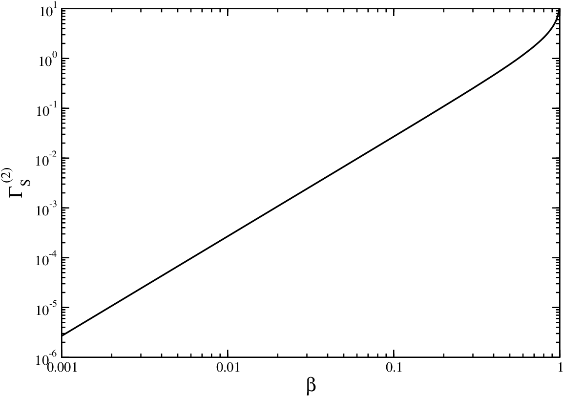
Figure 8: The two-loop cusp anomalous dimension, ΓS(2)\Gamma_{S}^{(2)}, as a function of β\beta in a linear (left) and logarithmic (right) plot.

Linear and logarithmic plots of ΓS(2)\Gamma_{S}^{(2)} are shown in Fig. 8. ΓS(2)\Gamma_{S}^{(2)} vanishes at β=0\beta=0, the threshold limit, and diverges at β=1\beta=1, the massless limit.

We next determine analytically the small and large β\beta behavior of ΓS(2)\Gamma_{S}^{(2)}. For the small β\beta behavior we expand around β=0\beta=0 and find

ΓS​exp(2)\displaystyle\Gamma_{S\,{\rm exp}}^{(2)} =\displaystyle= −227​β2​[CF​CA​(18​ζ2−47)+5​CF​nf]+𝒪⁡(β4).\displaystyle-\frac{2}{27}\beta^{2}\left[C_{F}C_{A}(18\zeta_{2}-47)+5C_{F}n_{f}\right]+{\cal O}(\beta^{4})\,.

We note that ΓS(2)\Gamma_{S}^{(2)} is an even function of β\beta. For the large β\beta behavior, as β→1\beta\rightarrow 1, we find ΓS(2)→K2​ΓS(1)\Gamma_{S}^{(2)}\rightarrow\frac{K}{2}\Gamma_{S}^{(1)}.

We next construct an approximation valid for all β\beta [16]:

ΓS​approx(2)\displaystyle\Gamma^{(2)}_{S\,{\rm approx}} =\displaystyle= ΓS​exp(2)+K2​ΓS(1)−K2​ΓS​exp(1)\displaystyle\Gamma^{(2)}_{S\,{\rm exp}}+\frac{K}{2}\Gamma_{S}^{(1)}-\frac{K}{2}\Gamma^{(1)}_{S\,{\rm exp}}
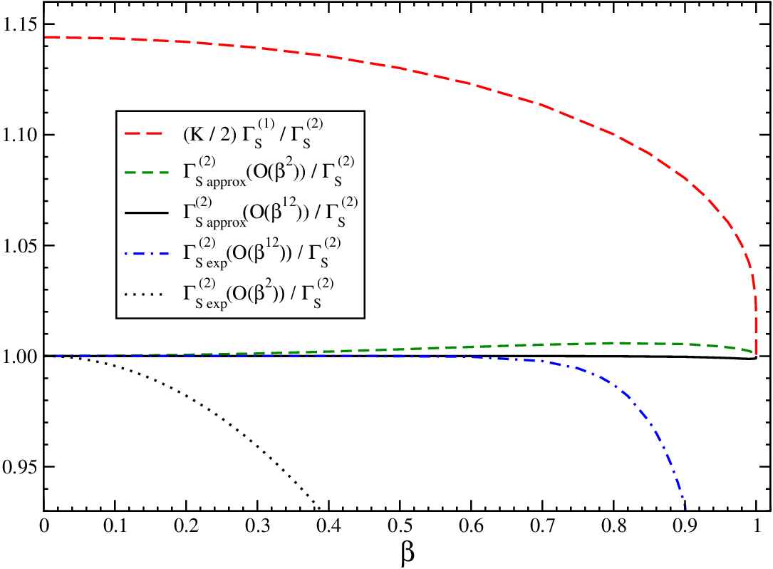
=\displaystyle= K2​ΓS(1)+CF​CA​(1−23​ζ2)​β2+𝒪⁡(β4).\displaystyle\frac{K}{2}\Gamma_{S}^{(1)}+C_{F}C_{A}\left(1-\frac{2}{3}\zeta_{2}\right)\beta^{2}+{\cal O}\left(\beta^{4}\right)\,.

Refer to caption

Figure 9: Expansions and approximations for ΓS(2)\Gamma_{S}^{(2)}.

The expansions and approximations to ΓS(2)\Gamma_{S}^{(2)} are shown in Fig. 9. ΓS​approx(2)\Gamma^{(2)}_{S\,{\rm approx}} is a remarkably good approximation to the complete ΓS(2)\Gamma_{S}^{(2)}.

4 Soft anomalous dimension matrices for t​t¯t{\bar{t}} production

Refer to caption     Refer to caption

Figure 10: Lowest-order diagrams for the q​q¯→t​t¯q{\bar{q}}\rightarrow t{\bar{t}} channel (left diagram) and the g​g→t​t¯gg\rightarrow t{\bar{t}} channel (right three diagrams).

The top-antitop pair production partonic processes at LO are

q⁡(p1)+q¯​(p2)→t⁡(p3)+t¯​(p4)q(p_{1})+{\bar{q}}(p_{2})\rightarrow t(p_{3})+{\bar{t}}(p_{4})

and

g⁡(p1)+g⁡(p2)→t⁡(p3)+t¯​(p4)g(p_{1})+g(p_{2})\rightarrow t(p_{3})+{\bar{t}}(p_{4})

The LO diagrams for these processes are shown in Fig. 10. We define s=(p1+p2)2s=(p_{1}+p_{2})^{2}, t1=(p1−p3)2−mt2t_{1}=(p_{1}-p_{3})^{2}-m_{t}^{2}, u1=(p2−p3)2−mt2u_{1}=(p_{2}-p_{3})^{2}-m_{t}^{2}, and β=1−4​mt2/s\beta=\sqrt{1-4m_{t}^{2}/s}. Note that β\beta is the top-quark speed in the LO kinematics. At the Tevatron and the LHC the t​t¯t{\bar{t}} cross section receives most contributions in the region around 0.3<β<0.80.3<\beta<0.8 which peak roughly around β∼0.6\beta\sim 0.6.

We next present the results at one and two loops for the soft anomalous matrices for these partonic processes. The soft anomalous dimension matrix for q⁡(p1)+q¯​(p2)→t⁡(p3)+t¯​(p4)q(p_{1})+{\bar{q}}(p_{2})\rightarrow t(p_{3})+{\bar{t}}(p_{4}) in a color tensor basis consisting of singlet and octet exchange in the ss channel,

c1=δ12​δ34,c2=TF​ 21c​TF​ 34c,\displaystyle c_{1}=\delta_{12}\delta_{34}\,,\quad\quad c_{2}=T^{c}_{F\;21}\,T^{c}_{F\;34}\,,

has elements

ΓSq​q¯→t​t¯=[Γq​q¯​ 11Γq​q¯​ 12Γq​q¯​ 21Γq​q¯​ 22].\displaystyle\Gamma_{S}^{q{\bar{q}}\rightarrow t{\bar{t}}}=\left[\begin{array}[]{cc}\Gamma_{q{\bar{q}}\,11}&\Gamma_{q{\bar{q}}\,12}\\ \Gamma_{q{\bar{q}}\,21}&\Gamma_{q{\bar{q}}\,22}\end{array}\right]\,.

At one loop we find [6, 19]

Γq​q¯​ 11(1)\displaystyle\Gamma_{q{\bar{q}}\,11}^{(1)} =\displaystyle= −CF​[Lβ+1]\displaystyle-C_{F}\,[L_{\beta}+1]
Γq​q¯​ 12(1)\displaystyle\Gamma_{q{\bar{q}}\,12}^{(1)} =\displaystyle= CFCA​ln⁡(t1u1)\displaystyle\frac{C_{F}}{C_{A}}\ln\left(\frac{t_{1}}{u_{1}}\right)
Γq​q¯​ 21(1)\displaystyle\Gamma_{q{\bar{q}}\,21}^{(1)} =\displaystyle= 2​ln⁡(t1u1)\displaystyle 2\ln\left(\frac{t_{1}}{u_{1}}\right)\hskip 42.67912pt
Γq​q¯​ 22(1)\displaystyle\Gamma_{q{\bar{q}}\,22}^{(1)} =\displaystyle= CF​[4​ln⁡(t1u1)−Lβ−1]+CA2​[−3​ln⁡(t1u1)+ln⁡(t1​u1s​mt2)+Lβ]\displaystyle C_{F}\left[4\ln\left(\frac{t_{1}}{u_{1}}\right)-L_{\beta}-1\right]+\frac{C_{A}}{2}\left[-3\ln\left(\frac{t_{1}}{u_{1}}\right)+\ln\left(\frac{t_{1}u_{1}}{sm_{t}^{2}}\right)+L_{\beta}\right]

where Lβ=1+β22​β​ln⁡(1−β1+β)L_{\beta}=\frac{1+\beta^{2}}{2\beta}\ln\left(\frac{1-\beta}{1+\beta}\right). We note that the first element of this matrix is identical to the one-loop massive cusp anomalous dimension.

Then the elements of the soft anomalous dimension matrix for the process q​q¯→t​t¯q{\bar{q}}\rightarrow t{\bar{t}} at two loops are [19]

Γq​q¯​ 11(2)\displaystyle\Gamma_{q{\bar{q}}\,11}^{(2)} =\displaystyle= K2​Γq​q¯​ 11(1)+CF​CA​Mβ\displaystyle\frac{K}{2}\Gamma_{q{\bar{q}}\,11}^{(1)}+C_{F}C_{A}\,M_{\beta}
Γq​q¯​ 12(2)\displaystyle\Gamma_{q{\bar{q}}\,12}^{(2)} =\displaystyle= K2​Γq​q¯​ 12(1)−CF2​Nβ​ln⁡(t1u1)\displaystyle\frac{K}{2}\Gamma_{q{\bar{q}}\,12}^{(1)}-\frac{C_{F}}{2}N_{\beta}\ln\left(\frac{t_{1}}{u_{1}}\right)
Γq​q¯​ 21(2)\displaystyle\Gamma_{q{\bar{q}}\,21}^{(2)} =\displaystyle= K2​Γq​q¯​ 21(1)+CA​Nβ​ln⁡(t1u1)\displaystyle\frac{K}{2}\Gamma_{q{\bar{q}}\,21}^{(1)}+C_{A}N_{\beta}\ln\left(\frac{t_{1}}{u_{1}}\right)
Γq​q¯​ 22(2)\displaystyle\Gamma_{q{\bar{q}}\,22}^{(2)} =\displaystyle= K2​Γq​q¯​ 22(1)+CA​(CF−CA2)​Mβ\displaystyle\frac{K}{2}\Gamma_{q{\bar{q}}\,22}^{(1)}+C_{A}\left(C_{F}-\frac{C_{A}}{2}\right)\,M_{\beta}

We note that the first element of this matrix is identical to the two-loop massive cusp anomalous dimension, and MβM_{\beta} was defined in the previous section. Here NβN_{\beta} is a subset of the terms of MβM_{\beta},

Nβ\displaystyle N_{\beta} =\displaystyle= −(1+β2)4​β​[ln2⁡(1−β1+β)+2​ln⁡(1−β1+β)​ln⁡((1+β)24​β)−Li2​((1−β)2(1+β)2)]\displaystyle-\frac{(1+\beta^{2})}{4\beta}\left[\ln^{2}\left(\frac{1-\beta}{1+\beta}\right)+2\ln\left(\frac{1-\beta}{1+\beta}\right)\ln\left(\frac{(1+\beta)^{2}}{4\beta}\right)-{\rm Li}_{2}\left(\frac{(1-\beta)^{2}}{(1+\beta)^{2}}\right)\right]
+12​ln2​(1−β1+β).\displaystyle{}+\frac{1}{2}\ln^{2}\left(\frac{1-\beta}{1+\beta}\right)\,.

The soft anomalous dimension matrix for g⁡(p1)+g⁡(p2)→t⁡(p3)+t¯​(p4)g(p_{1})+g(p_{2})\rightarrow t(p_{3})+{\bar{t}}(p_{4}) in a color tensor basis

c1=δ12​δ34,c2=d12​c​T34c,c3=i​f12​c​T34c\displaystyle c_{1}=\delta^{12}\,\delta_{34},\quad c_{2}=d^{12c}\,T^{c}_{34},\quad c_{3}=if^{12c}\,T^{c}_{34}

where dd and ff are the totally symmetric and antisymmetric S​U​(3)SU(3) invariant tensors, is

ΓSg​g→t​t¯=[Γg​g​ 110Γg​g​ 130Γg​g​ 22Γg​g​ 23Γg​g​ 31Γg​g​ 32Γg​g​ 22].\displaystyle\Gamma_{S}^{gg\rightarrow t{\bar{t}}}=\left[\begin{array}[]{ccc}\Gamma_{gg\,11}&0&\Gamma_{gg\,13}\\ 0&\Gamma_{gg\,22}&\Gamma_{gg\,23}\\ \Gamma_{gg\,31}&\Gamma_{gg\,32}&\Gamma_{gg\,22}\end{array}\right]\,.

At one loop we have [6, 19]

Γg​g​ 11(1)\displaystyle\Gamma_{gg\,11}^{(1)} =\displaystyle= −CF​[Lβ+1]\displaystyle-C_{F}[L_{\beta}+1]
Γg​g​ 13(1)\displaystyle\Gamma_{gg\,13}^{(1)} =\displaystyle= ln⁡(t1u1)\displaystyle\ln\left(\frac{t_{1}}{u_{1}}\right)
Γg​g​ 31(1)\displaystyle\Gamma_{gg\,31}^{(1)} =\displaystyle= 2​ln⁡(t1u1)\displaystyle 2\ln\left(\frac{t_{1}}{u_{1}}\right)
Γg​g​ 22(1)\displaystyle\Gamma_{gg\,22}^{(1)} =\displaystyle= −CF​[Lβ+1]+CA2​[ln⁡(t1​u1m2​s)+Lβ]\displaystyle-C_{F}[L_{\beta}+1]+\frac{C_{A}}{2}\left[\ln\left(\frac{t_{1}u_{1}}{m^{2}s}\right)+L_{\beta}\right]
Γg​g​ 23(1)\displaystyle\Gamma_{gg\,23}^{(1)} =\displaystyle= CA2​ln⁡(t1u1)\displaystyle\frac{C_{A}}{2}\ln\left(\frac{t_{1}}{u_{1}}\right)
Γg​g​ 32(1)\displaystyle\Gamma_{gg\,32}^{(1)} =\displaystyle= Nc2−42​Nc​ln⁡(t1u1)\displaystyle\frac{N_{c}^{2}-4}{2N_{c}}\ln\left(\frac{t_{1}}{u_{1}}\right)

At two loops we find [19]

Γg​g​ 11(2)\displaystyle\Gamma_{gg\,11}^{(2)} =\displaystyle= K2​Γg​g​ 11(1)+CF​CA​Mβ\displaystyle\frac{K}{2}\Gamma_{gg\,11}^{(1)}+C_{F}C_{A}\,M_{\beta}
Γg​g​ 13(2)\displaystyle\Gamma_{gg\,13}^{(2)} =\displaystyle= K2​Γg​g​ 13(1)−CA2​Nβ​ln⁡(t1u1)\displaystyle\frac{K}{2}\Gamma_{gg\,13}^{(1)}-\frac{C_{A}}{2}N_{\beta}\ln\left(\frac{t_{1}}{u_{1}}\right)
Γg​g​ 31(2)\displaystyle\Gamma_{gg\,31}^{(2)} =\displaystyle= K2​Γg​g​ 31(1)+CA​Nβ​ln⁡(t1u1)\displaystyle\frac{K}{2}\Gamma_{gg\,31}^{(1)}+C_{A}N_{\beta}\ln\left(\frac{t_{1}}{u_{1}}\right)
Γg​g​ 22(2)\displaystyle\Gamma_{gg\,22}^{(2)} =\displaystyle= K2​Γg​g​ 22(1)+CA​(CF−CA2)​Mβ\displaystyle\frac{K}{2}\Gamma_{gg\,22}^{(1)}+C_{A}\left(C_{F}-\frac{C_{A}}{2}\right)\,M_{\beta}
Γg​g​ 23(2)\displaystyle\Gamma_{gg\,23}^{(2)} =\displaystyle= K2​Γg​g​ 23(1)\displaystyle\frac{K}{2}\Gamma_{gg\,23}^{(1)}
Γg​g​ 32(2)\displaystyle\Gamma_{gg\,32}^{(2)} =\displaystyle= K2​Γg​g​ 32(1)\displaystyle\frac{K}{2}\Gamma_{gg\,32}^{(1)}

5 Double-differential kinematics

We consider a generic hadronic process with momenta ph1+ph2→p3+p4p_{h_{1}}+p_{h_{2}}\rightarrow p_{3}+p_{4} with underlying partonic process p1+p2→p3+p4p_{1}+p_{2}\rightarrow p_{3}+p_{4}. We write general kinematics formulas that can be used for both top-antitop pair and single-top production.

5.1 Kinematics with SS, TT, UU

The hadronic variables are S=(ph​1+ph​2)2S=(p_{h1}+p_{h2})^{2}, T=(ph​1−p3)2T=(p_{h1}-p_{3})^{2}, U=(ph​2−p3)2U=(p_{h2}-p_{3})^{2}. The partonic variables are s=(p1+p2)2s=(p_{1}+p_{2})^{2}, t=(p1−p3)2t=(p_{1}-p_{3})^{2}, u=(p2−p3)2u=(p_{2}-p_{3})^{2}; we also define s4=s+t+u−m32−m42s_{4}=s+t+u-m_{3}^{2}-m_{4}^{2} which describes the excess energy for additional radiation in the process, and thus measures kinematical distance from partonic threshold. Note that p1=x1​ph​1p_{1}=x_{1}p_{h1}, p2=x2​ph​2p_{2}=x_{2}p_{h2}, s=x1​x2​Ss=x_{1}x_{2}S, t−m32=x1​(T−m32)t-m_{3}^{2}=x_{1}(T-m_{3}^{2}), u−m32=x2​(U−m32)u-m_{3}^{2}=x_{2}(U-m_{3}^{2}), with x1x_{1} and x2x_{2} the momentum fractions of the colliding partons in the corresponding hadrons. The total hadronic cross section is found by integrating over the double-differential partonic cross section convoluted with the parton distribution functions ϕ\phi:

σph​1​ph​2→p3​p4​(S)\displaystyle\sigma_{p_{h1}p_{h2}\rightarrow p_{3}p_{4}}(S) =\displaystyle= ∫Tm​i​nTm​a​xd​T​∫Um​i​nUm​a​xd​U​∫x2​m​i​n1d​x2​∫0s4​m​a​xd​s4\displaystyle\int_{T_{min}}^{T_{max}}dT\int_{U_{min}}^{U_{max}}dU\int_{x_{2min}}^{1}dx_{2}\int_{0}^{s_{4max}}ds_{4}
×x1​x2x2​S+T−m32​ϕ​(x1)​ϕ​(x2)​d2​σ^p1​p2→p3​p4d​t​d​u\displaystyle\times\frac{x_{1}x_{2}}{x_{2}S+T-m_{3}^{2}}\,\phi(x_{1})\,\phi(x_{2})\,\frac{d^{2}{\hat{\sigma}}_{p_{1}p_{2}\rightarrow p_{3}p_{4}}}{dt\,du}

where

x1=s4−m32+m42−x2​(U−m32)x2​S+T−m32\displaystyle x_{1}=\frac{s_{4}-m_{3}^{2}+m_{4}^{2}-x_{2}(U-m_{3}^{2})}{x_{2}S+T-m_{3}^{2}}
Tm​i​nm​a​x=−12​(S−m32−m42)±12​(S−m32−m42)2−4​m32​m42\displaystyle T_{{}^{max}_{min}}=-\frac{1}{2}(S-m_{3}^{2}-m_{4}^{2})\pm\frac{1}{2}\sqrt{(S-m_{3}^{2}-m_{4}^{2})^{2}-4m_{3}^{2}m_{4}^{2}}
Um​a​x=m32+S​m32T−m32\displaystyle U_{max}=m_{3}^{2}+\frac{S\,m_{3}^{2}}{T-m_{3}^{2}}

Um​i​n=−S−T+m32+m42U_{min}=-S-T+m_{3}^{2}+m_{4}^{2}, x2​m​i​n=(m42−T)/(S+U−m32)x_{2min}=(m_{4}^{2}-T)/(S+U-m_{3}^{2}) and s4​m​a​x=x2​(S+U−m32)+T−m42s_{4max}=x_{2}(S+U-m_{3}^{2})+T-m_{4}^{2}.

5.2 Kinematics with pTp_{T} and rapidity

We next provide an alternative cross-section calculation in terms of the transverse momentum, pTp_{T}, and the rapidity, YY, of the outgoing particle with momentum p3p_{3}. We further define T1=T−m32T_{1}=T-m_{3}^{2}, U1=U−m32U_{1}=U-m_{3}^{2}, t1=t−m32t_{1}=t-m_{3}^{2}, and u1=u−m32u_{1}=u-m_{3}^{2}. Also, U1=−S​mT​eYU_{1}=-\sqrt{S}m_{T}e^{Y} and T1=−S​mT​e−YT_{1}=-\sqrt{S}m_{T}e^{-Y} with mT=m32+pT2m_{T}=\sqrt{m_{3}^{2}+p_{T}^{2}}. We then calculate the total hadronic cross section via

σph​1​ph​2→p3​p4​(S)\displaystyle\sigma_{p_{h1}p_{h2}\rightarrow p_{3}p_{4}}(S) =\displaystyle= ∫0pT​m​a​x2d​pT2​∫Y−Y+d​Y​∫x1−1d​x1​∫0s4​m​a​xd​s4\displaystyle\int_{0}^{p_{T\,max}^{2}}dp_{T}^{2}\int_{Y^{-}}^{Y^{+}}dY\int_{x_{1}^{-}}^{1}dx_{1}\int_{0}^{s_{4max}}ds_{4}
×x1​x2​Sx1​S+U1​ϕ​(x1)​ϕ​(x2)​d2​σ^p1​p2→p3​p4d​t1​d​u1\displaystyle\times\frac{x_{1}x_{2}\,S}{x_{1}S+U_{1}}\,\phi(x_{1})\,\phi(x_{2})\,\frac{d^{2}{\hat{\sigma}}_{p_{1}p_{2}\rightarrow p_{3}p_{4}}}{dt_{1}\,du_{1}}

where

x2=s4−m32+m42−x1​T1x1​S+U1,\displaystyle x_{2}=\frac{s_{4}-m_{3}^{2}+m_{4}^{2}-x_{1}T_{1}}{x_{1}S+U_{1}},
pT​m​a​x2=(S−m32−m42)2−4​m32​m424​S\displaystyle p_{T\,max}^{2}=\frac{(S-m_{3}^{2}-m_{4}^{2})^{2}-4m_{3}^{2}m_{4}^{2}}{4S}
Y±=±12​ln⁡1+1−4​mT2S​[1+(m32−m42)/S]21−1−4​mT2S​[1+(m32−m42)/S]2\displaystyle Y^{\pm}=\pm\frac{1}{2}\ln\frac{1+\sqrt{1-\frac{4m_{T}^{2}}{S[1+(m_{3}^{2}-m_{4}^{2})/S]^{2}}}}{1-\sqrt{1-\frac{4m_{T}^{2}}{S[1+(m_{3}^{2}-m_{4}^{2})/S]^{2}}}}
x1−=−(U1+m32−m42)S+T1\displaystyle x_{1}^{-}=\frac{-(U_{1}+m_{3}^{2}-m_{4}^{2})}{S+T_{1}}
s4​m​a​x=x1​(S+T1)+U1+m32−m42.\displaystyle s_{4max}=x_{1}(S+T_{1})+U_{1}+m_{3}^{2}-m_{4}^{2}\,.

6 Total cross section for t​t¯t{\bar{t}} production

Refer to caption     Refer to caption

Figure 11: (Left) NLO exact and approximate corrections to the top-pair cross section at 7 TeV (lower lines) and 8 TeV (upper lines) LHC energy; (Right) NLO exact and approximate top-quark transverse momentum distributions at 8 TeV.

Refer to caption     Refer to caption

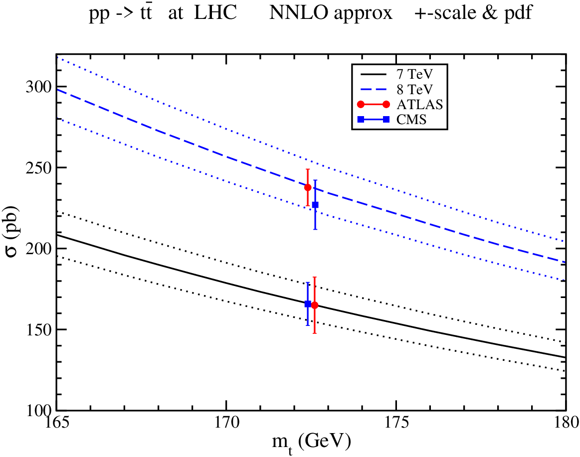
Figure 12: The top-pair total cross section at LHC (left) and Tevatron (right) energies.

We begin our presentation of numerical results with the total cross section for top-antitop pair production. We use the MSTW2008 NNLO [20] parton distribution functions (pdf) for all the numerical results. We first show that the threshold approximation works very well both for total cross sections and differential distributions.

We denote the NLO soft-gluon corrections from the expansion of the NNLL resummed cross section as NLO approximate corrections. Similarly the NNLO soft-gluon corrections are denoted as NNLO approximate corrections. Furthermore, the sum of the exact NLO cross section and the NNLO approximate corrections is denoted as the NNLO approximate cross section (and this applies to both total and differential cross sections).

Figure 11 shows that the NLO exact and approximate corrections to the total cross section as well as the top-quark pTp_{T} distribution are nearly identical. We have an excellent approximation: there is less than 1% difference between NLO approximate and exact cross sections. For the best prediction we add the NNLO approximate corrections to the exact NLO cross section. We find that that the scale dependence is greatly reduced when the NNLO approximate corrections are included.

In Fig. 12 we display theoretical predictions at approximate NNLO for the total cross section as a function of top-quark mass at the LHC (left plot) and the Tevatron (right plot) and compare them with data from the LHC at 7 TeV [21, 22] and 8 TeV [23, 24] and from the Tevatron at 1.96 TeV [25, 26]. We find very good agreement between the theoretical predictions and the data. The approximate NNLO prediction [19] for mt=173m_{t}=173 GeV is 7.08+0.20−0.24+0.36−0.277.08{}^{+0.20}_{-0.24}{}^{+0.36}_{-0.27} pb at the Tevatron at 1.96 TeV; 163+7−5±9163{}^{+7}_{-5}\pm 9 pb at the LHC at 7 TeV; 234+10−7±12234{}^{+10}_{-7}\pm 12 pb at 8 TeV LHC; and 920+50−39+33−35920{}^{+50}_{-39}{}^{+33}_{-35} pb at 14 TeV LHC. The central result is with μF=μR=mt\mu_{F}=\mu_{R}=m_{t}, the first uncertainty is from independent variation of μF\mu_{F} and μR\mu_{R} over the range mt/2m_{t}/2 to 2​mt2m_{t}, and the second uncertainty is from the MSTW2008 NNLO pdf at 90% CL. Of course the numerical results depend on the choice of pdf, αs\alpha_{s}, and choices of top quark mass and scales.

There are many differences between various resummation/NNLO approximate approaches in the literature and these have been detailed previously in [7, 27]. The differences include whether the resummation is for the total-only cross section versus for the double-differential cross section, whether it uses moment-space perturbative QCD (pQCD) versus Soft-Collinear Effective Theory (SCET), etc.

Refer to caption

Figure 13: Theoretical results for the t​t¯t{\bar{t}} cross section at 7 and 8 TeV LHC energies.

Resummations that only use the total cross section refer to production (or absolute) threshold and resum logarithms of β=1−4​mt2/s\beta=\sqrt{1-4m_{t}^{2}/s}. The soft limit here is the production threshold limit β→0\beta\rightarrow 0 (where the top quark velocities are zero), which is a special case of the more general partonic threshold. The partonic threshold is where there is just enough energy to produce the top quarks but they can have arbitrary pTp_{T} and are not restrained to be at rest. This more general double-differential approach to resummation can be expressed in single-particle-inclusive kinematics for the differential cross section d​σ/d​pT​d​yd\sigma/dp_{T}dy where the logarithms involve s4=s+t1+u1s_{4}=s+t_{1}+u_{1} and the soft limit is s4→0s_{4}\rightarrow 0.

The double-differential approach, in addition to using a more general definition of threshold, also allows the calculation of transverse momentum and rapidity distributions. For differential calculations, further differences between approaches arise from how the relation s+t1+u1=0s+t_{1}+u_{1}=0 is used in the plus-distribution coefficients, how subleading terms are treated, if/how damping factors are implemented to reduce the influence of contributions far from threshold, etc.

A comparison of various NNLO approximate approaches is shown in Fig. 13, all with the same choice of parameters, at 7 and 8 TeV LHC energies. In addition, exact NLO [3, 4] and NNLO [28] results for the total cross sections are also shown on the plot.

Ref. [19] uses our pQCD resummation formalism for the double-differential cross section. Ref. [29] uses pQCD resummation for the total-only cross section. Ref. [30] uses the SCET resummation formalism for the double-differential cross section. Ref. [31] uses the SCET resummation formalism for the total-only cross section. Lastly, Ref. [32] uses pQCD resummation for the total-only cross section.

Refer to caption   Refer to caption

Figure 14: Theoretical results for the t​t¯t{\bar{t}} cross section at the Tevatron (left) and at 14 TeV LHC energy (right).

Figure 14 shows the corresponding comparison for the Tevatron (left) and for 14 TeV LHC energy (right). One notes the varying degree of success of the various approaches in approximating the exact NNLO result.

The result in Ref. [19] from our formalism is very close to the exact NNLO [28] result: both the central values and the scale uncertainty are nearly the same and this holds true for all collider energies and top quark masses. This was expected from the comparison of exact and approximate corrections at NLO for both total and differential cross sections, and also from the comparison of approximate NNLO results in different kinematics in 2003 [33] (see also the discussions in [19] and [27]). There is less than 1% difference between approximate and exact cross sections at both NLO and NNLO.

The stability of the theoretical prediction over the past decade and the reliability of the NNLO approximate result and near-identical value to exact NNLO is very important for several reasons:

∙\bullet it provides confidence for applications to other processes (notably single-top production, WW production, and other processes);

∙\bullet it has been used extensively as a background for many analyses (Higgs searches, etc);

∙\bullet it means that we have reliable and near-exact NNLO pTp_{T} and rapidity distributions, which is important since at present there do not exist any exact NNLO results for differential distributions;

∙\bullet it suggests that NNNLO soft-gluon corrections may be good approximations to exact results at that order if/when they ever become available.

7 Top-quark pTp_{T} and rapidity distributions in t​t¯t{\bar{t}} production

We continue with top quark differential distributions in t​t¯t{\bar{t}} production. We present theoretical results for the top-quark transverse momentum and rapidity distributions at Tevatron and LHC energies.

7.1 Top-quark pTp_{T} distribution

Refer to caption     Refer to caption

Figure 15: The top quark pTp_{T} distribution at the Tevatron.

Refer to caption     Refer to caption

Figure 16: (Left) The top quark pTp_{T} distribution at the LHC at 7 and 8 TeV energies. (Right) The normalized top quark pTp_{T} distribution at 7 TeV LHC energy compared with ATLAS data in the dileptons channel.

Figure 15 displays the theoretical top quark pTp_{T} distribution at the Tevatron. A reduction in scale dependence relative to NLO is observed when the NNLO soft-gluon corrections are included. Excellent agreement of the NNLO approximate results with D0 data [34] can be seen over all the pTp_{T} range from the plot on the right. The theoretical results are also in good agreement with newer D0 data [35].

The top quark pTp_{T} distribution at LHC energies is shown on the left plot of Fig. 16 with two different choices of scale: mtm_{t} and mT=pT2+mt2m_{T}=\sqrt{p_{T}^{2}+m_{t}^{2}}. The right plot shows a comparison of the theoretical approximate NNLO normalized pTp_{T} distribution, (1/σ)​d​σ/d​pT(1/\sigma)d\sigma/dp_{T}, to recent ATLAS data [36] at 7 TeV energy up to pTp_{T} of 800 GeV.

Refer to caption     Refer to caption

Figure 17: The normalized top quark pTp_{T} distribution at 7 TeV LHC energy compared with CMS data in the ℓ\ell+jets channel (left) and the dileptons channel (right).

Figure 17 shows the same theoretical normalized top quark pTp_{T} distribution at the LHC compared to CMS data [37] at 7 TeV energy in the ℓ\ell+jets channel (left plot) and the dileptons channel (right plot). There is excellent agreement with CMS data, and the NNLO approximate result describes the data better than event generators (see the discussion in [37]); a similar conclusion is drawn in the comparison with CMS data at 8 TeV energy [38].

7.2 Top-quark rapidity distribution

Refer to caption     Refer to caption

Figure 18: The top quark rapidity distribution at the Tevatron (left) and the LHC (right).

The top-quark rapidity distribution has been calculated [39] for Tevatron energy (left plot in Fig. 18) and is in good agreement with recent data from D0 [35].

The top-quark forward-backward asymmetry is defined by

AFB=σ⁡(Y>0)−σ⁡(Y<0)σ⁡(Y>0)+σ⁡(Y<0).A_{\rm FB}=\frac{\sigma(Y>0)-\sigma(Y<0)}{\sigma(Y>0)+\sigma(Y<0)}\,.

The asymmetry is significant at the Tevatron. The theoretical result [39] for Tevatron energy is AFB=0.052−0.006+0.000A_{\rm FB}=0.052^{+0.000}_{-0.006} which is significantly smaller than observed values.

The theoretical top quark rapidity distribution at LHC energies [39] is shown in the right plot of Fig. 18 at NLO and approximate NNLO.

Refer to caption     Refer to caption

Figure 19: The normalized top quark rapidity distribution at 7 TeV LHC energy compared with CMS data in the ℓ\ell+jets channel (left) and the dileptons channel (right).

The normalized top quark rapidity distribution at the LHC at 7 TeV energy is shown in Fig. 19. Excellent agreement is found with CMS data at 7 TeV [37] and also at 8 TeV [38].

8 Single-top production

Refer to caption    Refer to caption    Refer to caption

Figure 20: LO diagrams for single-top production in the tt-channel (left diagram), ss-channel (second from left), and in t​WtW production (right two diagrams).

Single-top-quark production was first observed at the Tevatron in 2009 [40, 41]. The single-top partonic processes at LO are shown in Fig. 20.

The tt-channel processes are of the form q​b→q′​tqb\rightarrow q^{\prime}t and q¯​b→q¯′​t{\bar{q}}b\rightarrow{\bar{q}}^{\prime}t and are numerically dominant at Tevatron and LHC energies. The ss-channel processes are of the form q​q¯′→b¯​tq{\bar{q}}^{\prime}\rightarrow{\bar{b}}t and are small at both the Tevatron and the LHC. The associated t​WtW production proceeds via b​g→t​W−bg\rightarrow tW^{-} and is negligible at the Tevatron but significant (second largest) at the LHC. A related process to t​WtW production is the associated production of a charged Higgs boson with a top quark, b​g→t​H−bg\rightarrow tH^{-}.

8.1 tt-channel production

We begin with single top quark production in the tt-channel. This is the dominant single-top production channel at both Tevatron and LHC energies. The complete NLO corrections were calculated in [5].

The soft anomalous dimension matrix for tt-channel single top production at one and two loops has been calculated [42, 43]. The first element of this 2×22\times 2 matrix is given at one-loop by [42, 43]

ΓS​t−11(1)=CF​[ln⁡(−ts)+ln⁡(mt2−tmt​s)−12]\displaystyle{\Gamma}_{S\,t-11}^{(1)}=C_{F}\left[\ln\left(\frac{-t}{s}\right)+\ln\left(\frac{m_{t}^{2}-t}{m_{t}\sqrt{s}}\right)-\frac{1}{2}\right]

and at two loops by [43]

ΓS​t−11(2)=K2​ΓS​t−11(1)+CF​CA​(1−ζ3)4.\displaystyle\Gamma_{S\,t-11}^{(2)}=\frac{K}{2}\Gamma_{S\,t-11}^{(1)}+C_{F}C_{A}\frac{(1-\zeta_{3})}{4}\,.

Refer to caption     Refer to caption

Figure 21: The tt-channel total cross section (left); the top-quark pTp_{T} distribution in tt-channel production (right).

The left plot of Fig. 21 shows the total tt-channel cross section as a function of collider energy. Excellent agreement is found with D0 [44], CDF [45], CMS [46, 47], and ATLAS [48, 49] results.

LHC tt t¯{\bar{t}} Total (pb) 7 TeV 43.0+1.6−0.2±0.843.0{}^{+1.6}_{-0.2}\pm 0.8 22.9±0.5+0.7−0.922.9\pm 0.5{}^{+0.7}_{-0.9} 65.9+2.1−0.7+1.5−1.765.9{}^{+2.1}_{-0.7}{}^{+1.5}_{-1.7} 8 TeV 56.4+2.1−0.3±1.156.4{}^{+2.1}_{-0.3}\pm 1.1 30.7±0.7+0.9−1.130.7\pm 0.7{}^{+0.9}_{-1.1} 87.2+2.8−1.0+2.0−2.287.2{}^{+2.8}_{-1.0}{}^{+2.0}_{-2.2} 14 TeV 154+4−1±3154{}^{+4}_{-1}\pm 3 94+2−1+2−394{}^{+2}_{-1}{}^{+2}_{-3} 248+6−2+5−6248{}^{+6}_{-2}{}^{+5}_{-6}

Table 1: NNLO approximate tt-channel single-top and single-antitop cross sections with mt=173m_{t}=173 GeV. The first uncertainty is from scale variation between mt/2m_{t}/2 and 2​mt2m_{t} and the second uncertainty is from the MSTW2008 NNLO pdf [20] at 90% CL.

Table 1 lists the tt-channel single-top and single-antitop cross sections, and their sum, at 7, 8, and 14 TeV LHC energies, for a top quark mass mt=173m_{t}=173 GeV. The central results are with μF=μR=mt\mu_{F}=\mu_{R}=m_{t} and the first uncertainty is due to scale variation over the interval mt/2m_{t}/2 to 2​mt2m_{t}, while the second uncertainty denotes the pdf errors using MSTW2008 NNLO pdf at 90% CL. The theoretical ratio σ(t)/σ(t¯)=1.88−0.09+0.11\sigma(t)/\sigma({\bar{t}})=1.88{}^{+0.11}_{-0.09} at 7 TeV compares well with the ATLAS result of 1.81+0.23−0.221.81{}^{+0.23}_{-0.22} [50].

In addition to the total cross section, the top-quark pTp_{T} distribution in tt-channel production is of interest and has been calculated at NLO in [5, 51, 52, 53, 54]. More recently, approximate NNLO results based on NNLL resummation appeared in [55] (for another approach based on SCET, see [56]). The right plot of Fig. 21 shows the theoretical results for tt-channel top-quark pTp_{T} distributions at LHC energies [55].

8.2 ss-channel production

Refer to caption     Refer to caption

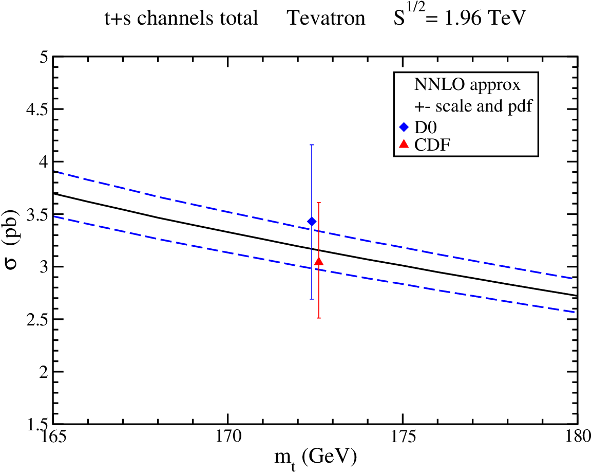
Figure 22: (Left) tt and ss channel combined cross sections compared with Tevatron data. (Right) ss-channel cross section at LHC energies.

LHC tt t¯{\bar{t}} Total (pb) 7 TeV 3.14±0.06+0.12−0.103.14\pm 0.06{}^{+0.12}_{-0.10} 1.42±0.01+0.06−0.071.42\pm 0.01{}^{+0.06}_{-0.07} 4.56±0.07+0.18−0.174.56\pm 0.07{}^{+0.18}_{-0.17} 8 TeV 3.79±0.07±0.133.79\pm 0.07\pm 0.13 1.76±0.01±0.081.76\pm 0.01\pm 0.08 5.55±0.08±0.215.55\pm 0.08\pm 0.21 14 TeV 7.87±0.14+0.31−0.287.87\pm 0.14{}^{+0.31}_{-0.28} 3.99±0.05+0.14−0.213.99\pm 0.05{}^{+0.14}_{-0.21} 11.86±0.19+0.45−0.4911.86\pm 0.19{}^{+0.45}_{-0.49}

Table 2: NNLO approximate ss-channel single-top and single-antitop cross sections with mt=173m_{t}=173 GeV. The first uncertainty is from scale variation between mt/2m_{t}/2 and 2​mt2m_{t} and the second uncertainty is from the MSTW2008 NNLO pdf [20] at 90% CL.

We continue with single top quark production in the ss-channel. The NLO corrections were calculated in [5].

The soft anomalous dimension matrix for this process has been calculated at one and two loops [42, 57]. The first element of this 2×22\times 2 matrix for ss-channel single top production at one loop is [42, 57]

ΓS​s−11(1)=CF​[ln⁡(s−mt2mt​s)−12]\displaystyle\Gamma_{S\,s-11}^{(1)}=C_{F}\left[\ln\left(\frac{s-m_{t}^{2}}{m_{t}\sqrt{s}}\right)-\frac{1}{2}\right]

and at two loops it is [57]

ΓS​s−11(2)=K2​ΓS​s−11(1)+CF​CA​(1−ζ3)4.\displaystyle\Gamma_{S\,s-11}^{(2)}=\frac{K}{2}\Gamma_{S\,s-11}^{(1)}+C_{F}C_{A}\frac{(1-\zeta_{3})}{4}\,.

Table 2 shows the single top and antitop ss-channel cross sections at the LHC for mt=173m_{t}=173 GeV. The NNLO approximate corrections provide an enhancement over NLO (with the same pdf) of ∼10\sim 10%.

In the left plot of Fig. 22 the sum of the tt and ss-channel cross sections at the Tevatron are displayed and compared with D0 [44] and CDF [45] data; the agreement is very good. The right plot of Fig. 22 shows the ss-channel cross section as a function of LHC energy together with the current limit from ATLAS [58].

Tevatron Total (pb) at 1.96 TeV tt-channel 2.08+0.00−0.04±0.122.08{}^{+0.00}_{-0.04}\pm 0.12 ss-channel 1.05+0.00−0.01±0.061.05{}^{+0.00}_{-0.01}\pm 0.06 t+st+s sum 3.13+0.00−0.05±0.183.13{}^{+0.00}_{-0.05}\pm 0.18

Table 3: NNLO approximate tt and ss channel total cross sections at the Tevatron with mt=173m_{t}=173 GeV.

Table 3 shows the single top and antitop tt-channel and ss-channel NNLO approximate cross sections at the Tevatron for mt=173m_{t}=173 GeV.

8.3 t​W−tW^{-} production

Refer to caption    Refer to caption    Refer to caption

Figure 23: Two-loop eikonal diagrams for t​WtW production.

We continue with the associated production of a top quark with a W−W^{-}. The NLO corrections for this process were calculated in [59]. The two-loop eikonal diagrams that contribute to the soft anomalous dimension are shown in Fig. 23 (additional top-quark self-energy graphs also contribute).

The soft anomalous dimension for b​g→t​W−bg\rightarrow tW^{-} is given at one loop by [42, 60]

ΓS​t​W−(1)=CF​[ln⁡(mt2−tmt​s)−12]+CA2​ln⁡(mt2−umt2−t)\displaystyle\Gamma_{S\,tW^{-}}^{(1)}=C_{F}\left[\ln\left(\frac{m_{t}^{2}-t}{m_{t}\sqrt{s}}\right)-\frac{1}{2}\right]+\frac{C_{A}}{2}\ln\left(\frac{m_{t}^{2}-u}{m_{t}^{2}-t}\right)

and at two loops by [60]

ΓS​t​W−(2)=K2​ΓS​t​W−(1)+CF​CA​(1−ζ3)4.\displaystyle\Gamma_{S\,tW^{-}}^{(2)}=\frac{K}{2}\Gamma_{S\,tW^{-}}^{(1)}+C_{F}C_{A}\frac{(1-\zeta_{3})}{4}\,.

Refer to caption     Refer to caption

Figure 24: Total cross section for t​WtW production (left); top-quark pTp_{T} distribution in t​W−tW^{-} production (right).

The left plot in Fig. 24 shows the total t​WtW cross section as a function of LHC energy together with LHC data at 7 TeV [61, 62] and 8 TeV [63, 64] energy. The agreement of data with theory is very good. The right plot displays the top-quark pTp_{T} distribution in t​W−tW^{-} production at LHC energies.

LHC t​W−tW^{-} (pb) 7 TeV 7.8±0.2+0.5−0.67.8\pm 0.2{}^{+0.5}_{-0.6} 8 TeV 11.1±0.3±0.711.1\pm 0.3\pm 0.7 14 TeV 41.8±1.0+1.5−2.441.8\pm 1.0{}^{+1.5}_{-2.4}

Table 4: NNLO approximate t​W−tW^{-} production cross sections with mt=173m_{t}=173 GeV.

Table 4 shows the cross sections for t​W−tW^{-} production at LHC energies for a top quark mass mt=173m_{t}=173 GeV. The NNLO approximate corrections increase the NLO cross section by ∼8\sim 8%. The cross section for t¯​W+{\bar{t}}W^{+} production is identical to that for t​W−tW^{-}.

8.4 Associated production of a top quark with a charged Higgs

Finally, we consider the production of a top quark in association with a charged Higgs boson [60]. Charged Higgs bosons appear in the Minimal Supersymmetric Standard Model (MSSM) and other two-Higgs doublet models. The soft anomalous dimension for this process is the same as for t​WtW production.

Refer to caption

Figure 25: Total cross sections for charged Higgs production in association with a top quark.

Figure 25 shows the cross section for t​H−tH^{-} production in the MSSM at LHC energies as a function of charged Higgs mass. The NNLO approximate corrections increase the NLO cross section by ∼15\sim 15 to ∼20\sim 20%, depending on the charged Higgs mass.

9 Summary

In these lectures I have presented higher-order calculations for top-quark production in hadronic collisions. I have discussed the resummation of soft-gluon corrections for top quark production via different partonic channels. NNLL resummation is achieved via two-loop eikonal calculations of soft anomalous dimension matrices. NNLO approximate results for the t​t¯t{\bar{t}} production cross section and the top quark pTp_{T} and rapidity distributions are in excellent agreement with data from the LHC and the Tevatron. Single top cross sections and pTp_{T} distributions have been presented in all partonic channels and are also in excellent agreement with collider data. The NNLO approximate corrections are very significant and they reduce the theoretical errors.

Acknowledgements

This material is based upon work supported by the National Science Foundation under Grant No. PHY 1212472.

References

  • [1] CDF Collaboration, Phys. Rev. Lett. 74, 2626 (1995) [hep-ex/9503002].
  • [2] D0 Collaboration, Phys. Rev. Lett. 74, 2632 (1995) [hep-ex/9503003].
  • [3] P. Nason, S. Dawson, and R.K. Ellis, Nucl. Phys. B 303, 607 (1988).
  • [4] W. Beenakker, H. Kuijf, W.L. van Neerven, and J. Smith, Phys. Rev. D 40, 54 (1989); W. Beenakker, W.L. van Neerven, R. Meng, G.A. Schuler, and J. Smith, Nucl. Phys. B 351, 507 (1991).
  • [5] B.W. Harris, E. Laenen, L. Phaf, Z. Sullivan, and S. Weinzierl, Phys. Rev. D 66, 054024 (2002) [hep-ph/0207055].
  • [6] N. Kidonakis and G. Sterman, Phys. Lett. B 387, 867 (1996); Nucl. Phys. B 505, 321 (1997) [hep-ph/9705234].
  • [7] N. Kidonakis and B.D. Pecjak, Eur. Phys. J. C 72, 2084 (2012) [arXiv:1108.6063 [hep-ph]].
  • [8] N. Kidonakis, Mod. Phys. Lett. A 19, 405 (2004) [hep-ph/0401147]; Phys. Rev. D 73, 034001 (2006) [hep-ph/0509079].
  • [9] G. Sterman, Nucl. Phys. B 281, 310 (1987).
  • [10] S. Catani and L. Trentadue, Nucl. Phys. B 327, 323 (1989).
  • [11] J. Kodaira and L. Trentadue, Phys. Lett. 112B, 66 (1982).
  • [12] H. Contopanagos, E. Laenen, and G. Sterman, Nucl. Phys. B 484, 303 (1997) [hep-ph/9604313].
  • [13] S. Moch, J.A.M. Vermaseren, and A. Vogt, Nucl. Phys. B 646, 181 (2002) [hep-ph/0209100]; Nucl. Phys. B 726, 317 (2005) [hep-ph/0506288].
  • [14] A. Gonzalez-Arroyo, C. Lopez, and F.J. Yndurain, Nucl. Phys. B 153, 161 (1979).
  • [15] G. Curci, W. Furmanski, and R. Petronzio, Nucl. Phys. B 175, 27 (1980).
  • [16] N. Kidonakis, Phys. Rev. Lett. 102, 232003 (2009) [arXiv:0903.2561 [hep-ph]].
  • [17] N. Kidonakis, arXiv:0910.0473 [hep-ph], in DPF 2009, eConf C090726.
  • [18] S.V. Ivanov, G.P. Korchemsky, and A.V. Radyushkin, Yad. Fiz. 44, 230 (1986) [Sov. J. Nucl. Phys. 44, 145 (1986)]; G.P. Korchemsky and A.V. Radyushkin, Phys. Lett. B 171, 459 (1986); Nucl. Phys. B 283, 342 (1987); Phys. Lett. B 279, 359 (1992) [hep-ph/9203222].
  • [19] N. Kidonakis, Phys. Rev. D 82, 114030 (2010) [arXiv:1009.4935 [hep-ph]].
  • [20] A.D. Martin, W.J. Stirling, R.S. Thorne, and G. Watt, Eur. Phys. J. C 63, 189 (2009) [arXiv:0901.0002 [hep-ph]].
  • [21] ATLAS Collaboration, ATLAS-CONF-2012-131.
  • [22] CMS Collaboration, CMS-PAS-TOP-11-024.
  • [23] ATLAS Collaboration, ATLAS-CONF-2013-097.
  • [24] CMS Collaboration, CMS-PAS-TOP-12-007.
  • [25] CDF Collaboration, Phys. Rev. D 82, 052002 (2010) [arXiv:1002.2919 [hep-ex]]; Conf. Note 10163.
  • [26] D0 Collaboration, Phys. Lett. B 679, 177 (2009) [arXiv:0901.2137 [hep-ex]]; Phys. Rev. D 82, 032002 (2010) [arXiv:0911.4286 [hep-ex]]; Phys. Lett. B 704, 403 (2011) [arXiv:1105.5384 [hep-ex]].
  • [27] N. Kidonakis, arXiv:1210.7813 [hep-ph] (to appear in Particles and Nuclei); in Snowmass 2013 Proceedings, SNOW13-00008 [arXiv:1304.7775 [hep-ph]]; PoS (EPS-HEP 2013) 432 [arXiv:1309.1442 [hep-ph]].
  • [28] M. Czakon, P. Fiedler, and A. Mitov, Phys. Rev. Lett. 110, 252004 (2013) [arXiv:1303.6254 [hep-ph]].
  • [29] M. Aliev, H. Lacker, U. Langenfeld, S. Moch, P. Uwer, and M. Wiedemann, Comput. Phys. Commun. 182, 1034 (2011) [arXiv:1007.1327 [hep-ph]].
  • [30] V. Ahrens, A. Ferroglia, M. Neubert, B.D. Pecjak, and L.L. Yang, Phys. Lett. B 703, 135 (2011) [arXiv:1105.5824 [hep-ph]].
  • [31] M. Beneke, P. Falgari, S. Klein, and C. Schwinn, Nucl. Phys. B 855, 695 (2012) [arXiv:1109.1536 [hep-ph]].
  • [32] M. Cacciari, M. Czakon, M. Mangano, A. Mitov, and P. Nason, Phys. Lett. B 710, 612 (2012) [arXiv:1111.5869 [hep-ph]].
  • [33] N. Kidonakis and R. Vogt, Phys. Rev. D 68, 114014 (2003) [hep-ph/0308222].
  • [34] D0 Collaboration, Phys. Lett. B 693, 515 (2010) [arXiv:1001.1900 [hep-ex]].
  • [35] D0 Collaboration, D0 Note 6379-CONF.
  • [36] ATLAS Collaboration, ATLAS-CONF-2013-099.
  • [37] CMS Collaboration, Eur. Phys. J. C 73, 2339 (2013) [arXiv:1211.2220 [hep-ex]].
  • [38] CMS Collaboration, CMS-PAS-TOP-12-028.
  • [39] N. Kidonakis, Phys. Rev. D 84, 011504 (2011) [arXiv:1105.5167 [hep-ph]].
  • [40] D0 Collaboration, Phys. Rev. Lett. 103, 092001 (2009) [arXiv:0903.0850 [hep-ex]].
  • [41] CDF Collaboration, Phys. Rev. Lett. 103, 092002 (2009) [arXiv:0903.0885 [hep-ex]].
  • [42] N. Kidonakis, Phys. Rev. D 74, 114012 (2006) [hep-ph/0609287].
  • [43] N. Kidonakis, Phys. Rev. D 83, 091503 (2011) [arXiv:1103.2792 [hep-ph]].
  • [44] D0 Collaboration, Phys. Rev. D 84, 112001 (2011) [arXiv:1108.3091 [hep-ex]].
  • [45] CDF Collaboration, CDF Note 10793.
  • [46] CMS Collaboration, JHEP 1212 (2012) 035 [arXiv:1209.4533 [hep-ex]].
  • [47] CMS Collaboration, CMS-PAS-TOP-12-011.
  • [48] ATLAS Collaboration, Phys. Lett. B 717, 330 (2012) [arXiv:1205.3130 [hep-ex]].
  • [49] ATLAS Collaboration, ATLAS-CONF-2012-132.
  • [50] ATLAS Collaboration, ATLAS-CONF-2012-056.
  • [51] J.M. Campbell, R. Frederix, F. Maltoni, and F. Tramontano, Phys. Rev. Lett. 102, 182003 (2009) [arXiv:0903.0005 [hep-ph]].
  • [52] R. Schwienhorst, C.-P. Yuan, C. Mueller, and Q.-H. Cao, Phys. Rev. D 83, 034019 (2011) [arXiv:1012.5132 [hep-ph]].
  • [53] P. Falgari, F. Giannuzzi, P. Mellor, and A. Signer, Phys. Rev. D 83, 094013 (2011) [arXiv:1102.5267 [hep-ph]].
  • [54] R. Frederix, E. Re, and P. Torrielli, JHEP 1209 (2012) 130 [arXiv:1207.5391 [hep-ph]].
  • [55] N. Kidonakis, Phys. Rev. D 88, 031504 (2013) [arXiv:1306.3592 [hep-ph]].
  • [56] J. Wang, C.S. Li, and H.X. Zhu, Phys. Rev. D 87, 034030 (2013) [arXiv:1210.7698 [hep-ph]].
  • [57] N. Kidonakis, Phys. Rev. D 81, 054028 (2010) [arXiv:1001.5034 [hep-ph]].
  • [58] ATLAS Collaboration, ATLAS-CONF-2011-118.
  • [59] S. Zhu, Phys. Lett. B 524, 283 (2002); (E) B 537, 351 (2002).
  • [60] N. Kidonakis, Phys. Rev. D 82, 054018 (2010) [arXiv:1005.4451 [hep-ph]].
  • [61] ATLAS Collaboration, Phys. Lett. B 716, 142 (2012) [arXiv:1205.5764 [hep-ex]].
  • [62] CMS Collaboration, Phys. Rev. Lett. 110, 022003 (2013) [arXiv:1209.3489 [hep-ex]].
  • [63] ATLAS Collaboration, ATLAS-CONF-2013-100.
  • [64] CMS Collaboration, CMS-PAS-TOP-12-040.