The Log-Volume of Optimal Codes for Memoryless Channels, Asymptotically Within A Few Nats

Pierre Moulin ^†^†thanks: The author is with the ECE Department, the Coordinated Science Laboratory, and the Beckman Institute at the University of Illinois at Urbana-Champaign, Urbana, IL 61801, USA. This research was initiated during the author’s sabbatical stay at the Chinese University of Hong Kong (January-March 2010) and supported by DARPA under the ITMANET program and by NSF under grant CCF 12-19145. This work was presented in part at the DARPA ITMANET meeting in Austin, TX, May 2010, at the ITA workshop in San Diego, CA, Feb. 2012, at ISIT in Cambridge, MA, July 2012, and at ISIT in Istanbul, Turkey, July 2013.

October 31, 2013.
Revised May 25, 2015, and June 11, 2016

Abstract

Shannon’s analysis of the fundamental capacity limits for memoryless communication channels has been refined over time. In this paper, the maximum volume $M_{\mathrm{avg}}^{*}(n,\epsilon)$ of length- $n$ codes subject to an average decoding error probability $\epsilon$ is shown to satisfy the following tight asymptotic lower and upper bounds as $n\to\infty$ :

\underline{A}_{\epsilon}+o(1)\leq\log M_{\mathrm{avg}}^{*}(n,\epsilon)-[nC-\sqrt{nV_{\epsilon}}\,Q^{-1}(\epsilon)+\frac{1}{2}\log n]\leq\overline{A}_{\epsilon}+o(1)

where $C$ is the Shannon capacity, $V_{\epsilon}$ the $\epsilon$ -channel dispersion, or second-order coding rate, $Q$ the tail probability of the normal distribution, and the constants $\underline{A}_{\epsilon}$ and $\overline{A}_{\epsilon}$ are explicitly identified. This expression holds under mild regularity assumptions on the channel, including nonsingularity. The gap $\overline{A}_{\epsilon}-\underline{A}_{\epsilon}$ is one nat for weakly symmetric channels in the Cover-Thomas sense, and typically a few nats for other symmetric channels, for the binary symmetric channel, and for the $Z$ channel. The derivation is based on strong large-deviations analysis and refined central limit asymptotics. A random coding scheme that achieves the lower bound is presented. The codewords are drawn from a capacity-achieving input distribution modified by an $O(1/\sqrt{n})$ correction term.

Keywords: Shannon theory, capacity, large deviations, local limit theorem, exponentially tilted distributions, binary symmetric channel, Z channel, Fisher information, Edgeworth expansion, random codes, Neyman-Pearson testing.

1 Introduction

Shannon’s seminal paper [2] introduced the fundamental capacity limits for memoryless communication channels. For any channel code of length $n$ and tolerable decoding error probability $\epsilon$ , the maximum volume of the code is given by $M^{*}(n,\epsilon)=e^{nC+o(n)}$ . The $o(n)$ term is significant for practical values of $n$ , hence much effort went into characterizing it in the early 1960’s [3, 4, 5, 6, 7]. It was discovered that under regularity conditions, the $o(n)$ term is of the form $-\sqrt{nV_{\epsilon}}\,Q^{-1}(\epsilon)+o(\sqrt{n})$ where $V_{\epsilon}$ is the $\epsilon$ -channel dispersion, or second-order coding rate. The $o(\sqrt{n})$ term was found to be $O(\log n)$ for discrete memoryless channels (DMCs), in a remarkable paper by Strassen [6] which pioneered the Neyman-Pearson (NP) hypothesis testing approach to the source and channel coding converse as well as the use of refined asymptotics for source and channel coding. This line of research seemed forgotten until its revival by Polyanskiy et al. [8, 9] and Hayashi [10]. Thus

\log M^{*}(n,\epsilon)=nC-\sqrt{nV_{\epsilon}}\,Q^{-1}(\epsilon)+O(\log n)

(1.1)

subject to some regularity conditions on the channel law. This holds under both the maximum and the average error probability criteria, and the corresponding maximum code volumes are denoted by $M_{\max}^{*}(n,\epsilon)$ and $M_{\mathrm{avg}}^{*}(n,\epsilon)$ , respectively.

The appeal of asymptotic expansions such as (1.1) is that they convey significant insights into the essence of the problem and they are practically useful. Indeed the remainder $O(\cdot)$ term can be bounded and sometimes neglected for moderately large values of $n$ , as shown numerically in [8].

The third-order term in (1.1) has been characterized in several studies. It is equal to $\frac{1}{2}\log n+O(1)$ for symmetric DMCs (see [6, footnote p. 692], which discusses a result by Dobrushin [5, Eqn. (75)]) and to $O(1)$ for the binary erasure channel (BEC). For DMCs with finite input alphabet ${\cal{X}}$ and output alphabet ${\cal{Y}}$ , under regularity assumptions on the channel law, the third-order term is sandwiched between $O(1)$ and $[1+o(1)](|{\cal{X}}|-\frac{1}{2})\log n$ [8]. If the DMC is nonsingular (has positive reverse dispersion), the third-order term is lower-bounded by $\frac{1}{2}\log n+O(1)$ [9, Sec. 3.4.5]. For the additive white Gaussian channel (AWGN) under an average (resp. maximum) power input constraint, the third-order term is sandwiched between $O(1)$ and $\frac{3}{2}\log n+O(1)$ (resp. $\frac{1}{2}\log n+O(1)$ ). More recent results on the third-order term, concurrent with the 2013 version of this manuscript [11], include a $\frac{1}{2}\log n+O(1)$ upper bound by Tomamichel and Tan [12] (using an $\epsilon$ hypothesis testing divergence approach and an auxiliary distribution that is a mixture of product distributions over ${\cal{Y}}^{n}$ ) and an $O(1)$ upper bound by Altug and Wagner [13] for singular DMCs. Haim et al. [14] recognized the importance of tie-breaking for ML decoding on the BSC, which presumably affects asymptotics beyond the third-order term. While the $\log n$ term is generally significant for moderate values of $n$ , the $O(1)$ term might be comparable to $\log n$ and is therefore of great interest as well in finite-blocklength analyses.

The state of the art in 2010 motivated us to undertake a more refined analysis of the problem, in which asymptotic equalities for the relevant error probabilities are obtained using strong large-deviations analysis, which are closely related to Laplace’s method for asymptotic expansion of integrals [15]—[18]. A strong large-deviations analysis provides an asymptotic expansion for the probability of rare events such as $\{\sum_{i=1}^{n}U_{i}\geq na\}$ where the random variables $U_{i},\,1\leq i\leq n$ are independent and identically distributed (iid), and $a$ is strictly larger than the mean of $U_{1}$ [19, 20]. Under regularity conditions, the expansion is of the form

\exp\left\{-n\Lambda(a)-\frac{1}{2}\log n+\gamma(a)+o(1)\right\}

where $\Lambda(\cdot)$ denotes the large-deviations function for $U_{1}$ and $\gamma(\cdot)$ is a real-valued function. In contrast, the ordinary (“weak”) large-deviations analysis merely states that the aforementioned probability vanishes as $\exp\{-n\Lambda(a)+o(n)\}$ . ¹¹ 1 The view expressed in [8, p. 2337]: “Inherently, the large deviations approach does not capture the subexponential behavior” applies only to the “weak” large-deviations analysis.

Using this approach, we derive the following sharp asymptotic bounds (Theorem 3.3). For channels with finite ${\cal{X}}$ and ${\cal{Y}}$ and positive dispersion, under regularity conditions, ²² 2 In the original version of this paper [11], stronger assumptions were given, including a unique capacity-achieving input distribution.

	$\displaystyle\underline{A}_{\epsilon}+o(1)$	$\displaystyle\leq$	$\displaystyle\log M_{\mathrm{avg}}^{*}(n,\epsilon)-\left[nC-\sqrt{nV_{\epsilon}}\,Q^{-1}(\epsilon)+\frac{1}{2}\log n\right]$		(1.2)
		$\displaystyle\leq$	$\displaystyle\overline{A}_{\epsilon}+o(1).$		(1.2)

Hence the third-order term in the asymptotic expansion is $\frac{1}{2}\log n$ , and the fourth-order term can be lower- and upper-bounded by two constants $\underline{A}_{\epsilon}$ and $\overline{A}_{\epsilon}$ that are easily computable and are independent of $n$ . The constant gap $\overline{A}_{\epsilon}-\underline{A}_{\epsilon}$ between the lower and upper bounds of (1.2) is equal to 1 nat for a class of symmetric channels. Moreover the gap is typically in the range 1—3 nats for other symmetric channels and for the nonsymmetric Z channel. This gap represents the “few nats” mentioned in the title of this paper.

The derivation of both the lower and upper bounds requires a refined analysis of the behavior of averages of independent random variables in the central regime. This analysis is rooted in two-term Edgeworth expansions [21, 22, 23, 24] and more specifically in work by Cramér [25] and Esséen [26] during the 1930’s and 1940’s. The Berry-Esséen theorem that was used by Strassen [6], Polyanskiy et al. [8], and Hayashi [10] provides a bound for deviation from Gaussianity but is not sharp enough for our purpose.

To obtain the lower bound in (1.2), we apply strong large deviations to analyze the error probability of random coding schemes with maximum-likelihood (ML) decoding. The only inequality used in this analysis is the classical union-of-events bound, which turns out to be remarkably tight.

To obtain the upper bound in (1.2), we use the technique introduced by Polyanskiy et al. [8] for proving converse theorems: it provides upper bounds for $M_{\max}^{*}(n,\epsilon)$ and $M_{\mathrm{avg}}^{*}(n,\epsilon)$ in terms of maxmin optimization problems whose payoff function is the type-II error probability of a NP test at significance level $1-\epsilon$ . This is a powerful idea which extends the NP-testing paradigm of Strassen [6, pp. 711, 712] and Kemperman [7, Theorem 7.1]. A key step in deriving our converse is to solve an asymptotic Neyman-Pearson game $\inf_{P}\sup_{Q}\beta_{n}(P,Q)$ where $P$ ranges over an $o(n^{-1/4})$ enlargement of the set of $\epsilon$ -dispersion-achieving input distributions, and $Q$ is a distribution on ${\cal{Y}}$ . We exploit this result to derive asymptotic upper bounds on $M_{\max}^{*}(n,\epsilon)$ and $M_{\mathrm{avg}}^{*}(n,\epsilon)$ ; we show that these asymptotic upper bounds are in fact identical. Prior work gave the inequality $M_{\mathrm{avg}}^{*}(n,\epsilon)\leq\sqrt{n}M_{\max}^{*}(n,\epsilon(1+n^{-1/2}))$ [8, p. 2332].

The paper is divided into nine sections and nine appendices and is organized as follows. Sec. 2 introduces the notation, basic definitions, and variational properties of information functions. Sec. 3 states the main result and applies it to a class of symmetric channels and to the (asymmetric) Z channel. Sec. 4 presents several optimization lemmas that are used throughout the paper. Sec. 5 reviews exact asymptotics in the central limit regime, in particular the Cramér-Esséen theorem, and strong large deviations asymptotics, with an emphasis on the general approach by Chaganty and Sethuramanan [27]. Sec. 6 presents new results on strong large deviations for likelihood ratios, including the case of varying component distributions (Sec. 6.1), and exact asymptotics of NP tests (Sec. 6.2). The lower bound on the log-volume of optimal codes is obtained via a random-coding argument in Sec. 7. The upper bound is obtained via a strong converse in Sec. 8. The paper concludes with a discussion in Sec. 9. For ease of reading, most proofs are presented in the appendices. The technical material relevant to the achievability results may be found in Sec. 1, Lemma 4.2, and Secs. 5.1, and 7. The material relevant to the converse includes everything but Sec. 7.

2 Preliminaries

2.1 Notation

We use uppercase letters for random variables, lowercase letters for their individual values, calligraphic letters for alphabets, boldface letters for sequences, and sans serif fonts for matrices. The set of all probability distributions on ${\cal{X}}$ is denoted by ${\mathscr{P}}({\cal{X}})$ . The support of a distribution $P$ is denoted by $\mathrm{supp}\{P\}$ . If ${\cal{X}}$ is discrete, $P$ is a probability mass function (pmf). Mathematical expectation, variance, and covariance with respect to $P$ are denoted by the symbols ${\mathbb{E}}_{P}$ , ${\mathrm{Var}}_{P}$ , and ${\mathrm{Cov}}_{P}$ , respectively. The probability density function (pdf) of the normal random variable is denoted by $\phi(x),\,x\in{\mathbb{R}}$ and the cumulative distribution function (cdf) by $\Phi(x)=1-Q(x)$ .

The indicator function of a set ${\cal{A}}$ is denoted by $\mathds{1}\{x\in{\cal{A}}\}$ . All logarithms are natural logarithms. The symbol $\mathrm{Proj}_{\cal{V}}(\cdot)$ denotes orthogonal projection onto a vector space ${\cal{V}}$ .

The symbol $f(n)\sim g(n)$ denotes asymptotic equality: $\lim_{n\rightarrow\infty}\frac{f(n)}{g(n)}=1$ . The notation $f(n)=o(g(n))$ (small oh, also denoted by $f(n)\ll g(n)$ ) indicates that $\lim_{n\rightarrow\infty}\frac{f(n)}{g(n)}=0$ . The notation $f(n)=O(g(n))$ indicates that $\limsup_{n\rightarrow\infty}|\frac{f(n)}{g(n)}|<\infty$ . In case the sequences $f(n)$ and $g(n)$ depend on a variable $P$ lying in a set ${\mathscr{P}}_{n}$ (possibly dependent on $n$ ), the same symbols are used to denote uniform convergence over $\{{\mathscr{P}}_{n}\}_{n\geq 1}$ , e.g., $f(P,n)=o(g(P,n))$ indicates that $\lim_{n\rightarrow\infty}\sup_{P\in{\mathscr{P}}_{n}}\frac{f(P,n)}{g(P,n)}=0$ .

Consider a DMC $(W,{\cal{X}},{\cal{Y}})$ with input and output alphabets ${\cal{X}}$ and ${\cal{Y}}$ respectively and conditional pmf $W(\cdot|x)\in{\mathscr{P}}({\cal{Y}})$ , also denoted by $W_{x}(\cdot)$ , for each $x\in{\cal{X}}$ . Given an input pmf $P$ on ${\cal{X}}$ , denote by $P\times W$ the joint pmf on ${\cal{X}}\times{\cal{Y}}$ and by $(PW)$ the marginal output pmf, i.e.,

(PW)(y)\triangleq\sum_{x\in{\cal{X}}}P(x)W(y|x)\quad\forall y\in{\cal{Y}}.

Kullback-Leibler (KL) divergence between two distributions $P$ and $Q$ on a common alphabet is denoted by $D(P\|Q)\triangleq{\mathbb{E}}_{P}[\log\frac{dP}{dQ}]$ , divergence variance by $V(P\|Q)\triangleq{\mathbb{E}}_{P}[\log\frac{dP}{dQ}]^{2}-D^{2}(P\|Q)$ , and divergence centralized third moment by $T(P\|Q)\triangleq{\mathbb{E}}_{P}[\log\frac{dP}{dQ}-D(P\|Q)]^{3}$ . Rényi divergence of order $\alpha\neq 1$ is denoted by $D_{\alpha}(P\|Q)=\frac{1}{\alpha-1}\log{\mathbb{E}}_{Q}[\frac{dP}{dQ}]^{\alpha}$ ; recall that $\lim_{\alpha\to 1}D_{\alpha}(P\|Q)=D(P\|Q)$ .

Given two alphabets ${\cal{X}}$ and ${\cal{Y}}$ , a ${\cal{X}}$ -valued random variable $X$ distributed as $P$ , and two conditional distributions $W$ and $Q$ on a ${\cal{Y}}$ -valued random variable $Y$ given $X$ , denote by $D(W\|Q|P)={\mathbb{E}}_{P\times W}\left[\log\frac{W(Y|X)}{Q(Y|X)}\right]$ the conditional KL divergence between $W$ and $Q$ given $P$ , and likewise by $V(W\|Q|P)={\mathbb{E}}_{P}[V(W_{X}\|Q)]$ and $T(W\|Q|P)={\mathbb{E}}_{P}[T(W_{X}\|Q)]$ the conditional divergence variance and the conditional divergence third central moment. Conditional Rényi divergence of order $\alpha\neq 1$ is defined as $D_{\alpha}(W\|Q|P)\triangleq{\mathbb{E}}_{P}[D_{\alpha}(W_{X}\|Q)]$ [28].

2.2 Definitions

We review some standard definitions. A real random variable $L$ is said to be of the lattice type if there exist numbers $d$ and $l_{0}$ such that $L$ belongs to the lattice $\{l_{0}+kd,\,k\in{\mathbb{Z}}\}$ with probability 1. The largest $d$ for which this holds is called the span of the lattice, and $l_{0}$ is the offset. The sum of a nonlattice random variable and an independent lattice random variable is a nonlattice random variable. The sum of two independent lattice random variables is a lattice random variable if and only if the ratio of their spans is a rational number. For each $d>0$ , define the discrete set

{\mathscr{P}}_{\textrm{lat}}(d)\triangleq\left\{Q\in{\mathscr{P}}({\cal{Y}})~:~\log\frac{W(Y|X)}{Q(Y)}\mathrm{~is~a~lattice~rv~with~span~}d\right\}.

(2.1)

The union of these sets over all $d>0$ forms a sieve for ${\mathscr{P}}({\cal{Y}})$ , where $d$ is the mesh size.

The information density is defined as

i(x,y)=\log\frac{W(y|x)}{(PW)(y)},\quad x\in{\cal{X}},y\in{\cal{Y}}.

(2.2)

For some DMCs with capacity-achieving input distribution, the random variable $i(X,Y)$ is of the lattice type. For instance $i(X,Y)\in\{\log(2\theta),\,\log(2-2\theta)\}$ for the BSC with crossover probability $\theta\neq\{0,\frac{1}{2},1\}$ and uniform input distribution; the span of the lattice is $\log|\frac{\theta}{1-\theta}|$ . However for almost every asymmetric binary channel, as well as for almost every nonbinary channel (symmetric or not), $i(X;Y)$ is not of the lattice type. We refer to capacity problems where $i(X,Y)$ is of the lattice type as the lattice case.

The following moments of the random variable $i(X,Y)$ with respect to the joint distribution $P\times W$ are used throughout this paper: the unconditional mean (= mutual information)

\displaystyle I(P;W)={\mathbb{E}}_{P\times W}[i(X,Y)]

\displaystyle=

\displaystyle D(P\times W\|P\times(PW)),

(2.3)

the conditional mean (given $X=x$ )

D(W_{x}\|(PW))={\mathbb{E}}_{W_{x}}[i(x,Y)],\quad x\in{\cal{X}},

the unconditional information variance

\displaystyle V_{\mathrm{u}}(P;W)={\mathrm{Var}}_{P\times W}[i(X,Y)]

\displaystyle=

\displaystyle V(P\times W\|P\times(PW)),

(2.4)

the conditional information variance (given $X$ )

\displaystyle V(P;W)

\displaystyle=

\displaystyle{\mathbb{E}}\{{\mathrm{Var}}[i(X,Y)|X]\}=\sum_{x\in{\cal{X}}}P(x)V(W_{x}\|PW),

(2.5)

the reverse dispersion [8, p. 89]

V^{r}(P;W)={\mathbb{E}}\{{\mathrm{Var}}[i(X,Y)|Y]\},

(2.6)

the unconditional third central moment

\displaystyle T_{\mathrm{u}}(P;W)

\displaystyle=

\displaystyle T(P\times W\|P\times(PW)),

(2.7)

the conditional third central moment (given $X$ )

\displaystyle T(P;W)

\displaystyle=

\displaystyle\sum_{x\in{\cal{X}}}P(x)T(W_{x}\|PW),

(2.8)

the unconditional skewness

S_{\mathrm{u}}(P;W)=\frac{T_{\mathrm{u}}(P;W)}{[V_{\mathrm{u}}(P;W)]^{3/2}},

(2.9)

and the conditional skewness

S(P;W)=\frac{T(P;W)}{[V(P;W)]^{3/2}}.

(2.10)

It follows from these definitions that

V(P;W)=V(W\|(PW)|P)\quad\mathrm{and}\quad T(P;W)=T(W\|(PW)|P).

(2.11)

Define the shorthand $t_{\epsilon}=Q^{-1}(\epsilon)$ . The following functions will also be used throughout:

F_{\epsilon}(W\|Q|P)\triangleq\frac{1}{2}t_{\epsilon}^{2}-\frac{1}{6}\frac{T(W\|Q|P)}{V(W\|Q|P)}(t_{\epsilon}^{2}-1)+\frac{1}{2}\log(2\pi V(W\|Q|P))

(2.12)

and

\zeta_{n}(P,Q)\triangleq nD(W\|Q|P)-\sqrt{nV(W\|Q|P)}\,t_{\epsilon}+F_{\epsilon}(W\|Q|P)

(2.13)

where $P\in{\mathscr{P}}({\cal{X}})$ and $Q\in{\cal{Q}}\triangleq\{Q=(PW):~P\in{\mathscr{P}}({\cal{X}})\}\subset{\mathscr{P}}({\cal{Y}})$ . Evaluating (2.12) and (2.13) at $Q=(PW)$ and using (2.11), we obtain the functions

F_{\epsilon}(P;W)\triangleq\frac{1}{2}t_{\epsilon}^{2}-\frac{1}{6}\frac{T(P;W)}{V(P;W)}(t_{\epsilon}^{2}-1)+\frac{1}{2}\log(2\pi V(P;W))

(2.14)

and

	$\displaystyle\zeta_{n}(P;W)$	$\displaystyle\triangleq$	$\displaystyle nI(P;W)-\sqrt{nV(P;W)}\,t_{\epsilon}+F_{\epsilon}(P,W)$		(2.15)
		$\displaystyle=$	$\displaystyle\zeta_{n}(P,(PW)).$		(2.15)

Shannon capacity is given by $C=\sup_{P\in{\mathscr{P}}({\cal{X}})}I(P;W)$ . Denote by $Q^{*}\in{\mathscr{P}}({\cal{Y}})$ the capacity-achieving output distribution, which is unique. Define the set of capacity-achieving input distributions

\Pi\triangleq\{P\in{\mathscr{P}}({\cal{X}}):~(PW)=Q^{*}\}

(2.16)

and the vector $\Delta$ with components

\Delta(x)=D(W_{x}\|Q^{*})-C,\quad x\in{\cal{X}}.

(2.17)

Let ${\mathcal{X}_{\mathrm{cap}}}\triangleq\{x\in{\cal{X}}:~\Delta(x)=0\}$ . It is well known that $\Delta(x)\leq 0$ for all $x\in{\cal{X}}$ and that $\mathrm{supp}(P)\subseteq{\mathcal{X}_{\mathrm{cap}}}$ is a necessary condition for $P\in\Pi$ . With a slight abuse of notation, we define ${\mathscr{P}}({\mathcal{X}_{\mathrm{cap}}})\triangleq\{P\in{\mathscr{P}}({\cal{X}}):\mathrm{supp}(P)\subseteq{\mathcal{X}_{\mathrm{cap}}}\}$ .

For $P\in\Pi$ , we have $V(P;W)=\sum_{x}P(x)\tilde{v}(x)$ where $\tilde{v}(x)\triangleq V(W_{x}\|Q^{*})$ . Moreover the gradient of $V(P;W)$ , for $P\in\Pi$ , is given by $\frac{\partial V(P;W)}{\partial P(x)}=\tilde{v}(x)$ , $x\in{\cal{X}}$ . Define

V_{\min}\triangleq\min_{P\in\Pi}V(P;W),\quad V_{\max}\triangleq\max_{P\in\Pi}V(P;W),

(2.18)

the $\epsilon$ channel dispersion

V_{\epsilon}=\begin{cases}V_{\min}&:\,\epsilon\leq\frac{1}{2}\\ V_{\max}&:\,\mathrm{else,}\end{cases}

(2.19)

and the subset of $\epsilon$ -dispersion-achieving distributions

\Pi^{*}\triangleq\left\{P\in\Pi:~\sum_{x\in{\cal{X}}}P(x)\tilde{v}(x)=V_{\epsilon}\right\}:\quad\epsilon\neq\frac{1}{2}

(2.20)

and $\Pi^{*}=\Pi$ if $\epsilon=\frac{1}{2}$ . Both $\Pi$ and $\Pi^{*}$ are convex polytopes. For $\epsilon\neq\frac{1}{2}$ , the set $\Pi^{*}$ is generally a singleton, except on a set of channels of measure zero. Any dispersion-achieving input distribution has support in the following subset of ${\mathcal{X}_{\mathrm{cap}}}$ :

{\cal{X}}^{*}\triangleq\cup_{P\in\Pi^{*}}\mathrm{supp}(P).

(2.21)

We will extensively use the following $\delta$ -enlargements of the sets $\Pi$ and $\Pi^{*}$ :

	$\displaystyle\Pi(\delta)$	$\displaystyle\triangleq$	$\displaystyle\{P\in{\mathscr{P}}({\cal{X}}):\min_{P^{\prime}\in\Pi}\\|P-P^{\prime}\\|_{\infty}\leq\delta\},$		(2.22)
	$\displaystyle\Pi^{*}(\delta)$	$\displaystyle\triangleq$	$\displaystyle\{P\in{\mathscr{P}}({\cal{X}}):\min_{P^{\prime}\in\Pi^{*}}\\|P-P^{\prime}\\|_{\infty}\leq\delta\},\quad\delta>0.$		(2.23)

Define the reverse channel with input distribution $(PW)$ and output distribution $P$ as

\widecheck{W}(x|y)\triangleq\frac{W(y|x)\,P(x)}{(PW)(y)},\quad x\in{\cal{X}},\,y\in{\cal{Y}}.

(2.24)

Also define

\rho(P;W)\triangleq 1-\frac{V^{r}(P;W)}{V_{\mathrm{u}}(P;W)},

(2.25)

which will be interpreted in Sec. 7 as a normalized correlation coefficient. For now, note that $\rho(P;W)\in[0,1]$ as a consequence of the law of total variance:

	$\displaystyle{\mathrm{Var}}[i(X;Y)]$	$\displaystyle=$	$\displaystyle{\mathbb{E}}\{{\mathrm{Var}}[i(X;Y)\|Y]\}+{\mathrm{Var}}[{\mathbb{E}}(i(X;Y)\|Y)]$
	$\displaystyle\Rightarrow\quad V_{\mathrm{u}}(P;W)$	$\displaystyle=$	$\displaystyle V^{r}(P;W)+{\mathrm{Var}}_{(PW)}[D(\widecheck{W}_{Y}\\|P)].$		(2.26)

A DMC $(W,{\cal{X}},{\cal{Y}})$ is said to be weakly symmetric in the Cover-Thomas (CT) sense if the rows $W_{x}(\cdot)$ of the channel transition probability matrix are permutations of each other and all the column sums are equal. See [30] for a detailed discussion of symmetric channels.

The empirical distribution on ${\cal{X}}$ ( $n$ -type) of a sequence ${\mathbf{x}}\in{\cal{X}}^{n}$ is defined by

\hat{P}_{\mathbf{x}}(x)\triangleq\frac{1}{n}\sum_{i=1}^{n}\mathds{1}\{x_{i}=x\},\quad x\in{\cal{X}}.

(2.27)

We denote by ${\mathscr{P}}_{n}({\cal{X}})\triangleq\{\hat{P}_{\mathbf{x}},\,{\mathbf{x}}\in{\cal{X}}^{n}\}$ the set of $n$ -types.

2.3 Encoder, Decoder, and Error Probabilities

The message $m$ to be transmitted is drawn uniformly from the message set ${\cal{M}}_{n}=\{1,2,\cdots,M_{n}\}$ . A deterministic code is a pair of encoder mapping $f_{n}~:~{\cal{M}}_{n}\to{\mathsf{F}}\subset{\cal{X}}^{n}$ , ${\mathbf{x}}(m)=f_{n}(m)$ , and decoder mapping $g_{n}~:~{\cal{Y}}^{n}\to{\cal{M}}_{n}$ , $\hat{m}=g_{n}({\mathbf{y}})$ . The code has volume (or size) $M_{n}$ and rate $R_{n}\triangleq\frac{1}{n}\log M_{n}$ . More generally, we assume a stochastic encoder where the codeword assigned to message $m$ is drawn from a conditional probability distribution $P_{{\mathbf{X}}|M=m}$ , and a stochastic decoder whose output $\widehat{M}\in{\cal{M}}_{n}$ is drawn from a conditional distribution $P_{\widehat{M}|{\mathbf{Y}}}$ .

The error probability for message $m\in{\cal{M}}_{n}$ is given by

e(m)\triangleq\sum_{{\mathbf{x}}\in{\cal{X}}^{n}}P_{{\mathbf{X}}|M}({\mathbf{x}}|m)\sum_{{\mathbf{y}}\in{\cal{Y}}^{n}}W^{n}({\mathbf{y}}|{\mathbf{x}})[1-P_{\widehat{M}|{\mathbf{Y}}}(m|{\mathbf{y}})].

Both the average error probability

P_{e,\mathrm{avg}}(f_{n},g_{n},W)\triangleq\frac{1}{M_{n}}\sum_{m\in{\cal{M}}_{n}}e(m)

and the maximum error probability

P_{e,\max}(f_{n},g_{n},W)\triangleq\max_{m\in{\cal{M}}_{n}}e(m)

are considered in this paper. For $n\geq 1$ and $\epsilon\in(0,1)$ , denote by

M_{\mathrm{avg}}^{*}(n,\epsilon)\triangleq\max\{M_{n}~:~\exists(f_{n},g_{n})~:~P_{e,\mathrm{avg}}(f_{n},g_{n},W)\leq\epsilon\}

and

M_{\max}^{*}(n,\epsilon)\triangleq\max\{M_{n}~:~\exists(f_{n},g_{n})~:~P_{e,\max}(f_{n},g_{n},W)\leq\epsilon\}

the maximum possible value of $M_{n}$ for arbitrary $(n,\epsilon)$ codes under the average and maximum error probability criteria, respectively. We will also consider constant-composition codes, which are particularly useful in problems with maximum-cost constraints on the codewords [17].

2.4 Fisher Information Matrix

Since $I(P;W)$ is a concave function of $P$ , its Hessian is nonnegative definite. Moreover, if $P^{*}$ is the unique maximizer of $I(\cdot;W)$ , the Hessian at $P^{*}$ is positive definite. The gradient of $I(P;W)$ is given by

\frac{\partial I(P;W)}{\partial P(x)}=D(W_{x}\|(PW))-1,\quad x\in{\cal{X}}

(2.28)

and the negative Hessian by

	$\displaystyle J_{xx^{\prime}}^{\cal{X}}(P,W)\triangleq-\frac{\partial^{2}I(P;W)}{\partial P(x)\partial P(x^{\prime})}$	$\displaystyle=$	$\displaystyle-\frac{\partial D(W_{x}\\|(PW))}{\partial P(x^{\prime})}$		(2.29)
		$\displaystyle=$	$\displaystyle\sum_{y\in{\cal{Y}}}\frac{W(y\|x)\,W(y\|x^{\prime})}{(PW)(y)},\quad\forall x,x^{\prime}\in{\cal{X}}.$		(2.29)

This expression was already derived by Strassen [6, below (4.43)] and can be interpreted as the Fisher information matrix for the probability vector $P$ given $Y$ [11]. The matrix $J^{\cal{X}}(P;W)$ is symmetric and nonnegative definite, and factorizes as $J^{\cal{X}}(P;W)={\mathsf{L}}{\mathsf{L}}^{\top}$ where

{\mathsf{L}}(x,y)=\frac{W(y|x)}{\sqrt{(PW)(y)}},\quad x\in{\cal{X}},y\in{\cal{Y}}.

(2.30)

Moreover

\sum_{x\in{\cal{X}}}P(x^{\prime})J_{xx^{\prime}}^{\cal{X}}(P,W)=1,\quad\forall x\in{\cal{X}}.

(2.31)

The matrix $J^{\cal{X}}(P;W)$ is the same for all $P\in\Pi$ , and we denote it by ${\mathsf{J}}^{\cal{X}}$ for short. However, only its entries indexed by $x,x^{\prime}\in{\cal{X}}^{*}$ of (2.21) will affect the fourth-order term. ³³ 3 In Sec. 4, we also use the entries indexed by $x,x^{\prime}\in{\mathcal{X}_{\mathrm{cap}}}$ . We therefore define a $|{\cal{X}}|\times|{\cal{X}}|$ matrix ${\mathsf{J}}\succeq 0$ as follows. If ${\cal{X}}={\cal{X}}^{*}$ , then ${\mathsf{J}}=J^{\cal{X}}$ . Else ${\mathsf{J}}$ coincides with $J^{\cal{X}}(P;W)$ for $x,x^{\prime}\in{\cal{X}}^{*}$ and is zero elsewhere. Therefore $\mathrm{rank}({\mathsf{J}})\leq|{\cal{X}}^{*}|$ . Now define the following subspaces of ${\mathbb{R}}^{\cal{X}}$ :

	$\displaystyle{\mathscr{L}}({\cal{X}})$	$\displaystyle\triangleq$	$\displaystyle\{h\in{\mathbb{R}}^{{\cal{X}}}:\sum_{x\in{\cal{X}}}h(x)=0\},$		(2.32)
	$\displaystyle{\mathscr{L}}({\cal{X}}^{*})$	$\displaystyle\triangleq$	$\displaystyle\{h\in{\mathscr{L}}({\cal{X}}):\mathrm{supp}(h)\subseteq{\cal{X}}^{*}\}.$		(2.33)

We have

h^{\top}{\mathsf{J}}^{\cal{X}}h={\mathbb{E}}_{Q^{*}}\left(\frac{(hW)(Y)}{Q^{*}(Y)}\right)^{2}\geq 0,\quad\forall h\in{\mathscr{L}}({\cal{X}})

(2.34)

where $(hW)(y)\triangleq\sum_{x\in{\cal{X}}}h(x)W(y|x)$ . We refer to $\|h\|_{\mathsf{J}}\triangleq\sqrt{h^{\top}{\mathsf{J}}h}$ , $h\in{\mathscr{L}}({\cal{X}})$ as the Fisher information metric associated with $\{W(y|x)\}_{x\in{\cal{X}}^{*},y\in{\cal{Y}}}$ , and to $h^{\top}{\mathsf{J}}\tilde{h}$ , $h,\tilde{h}\in{\mathscr{L}}({\cal{X}})$ , as the Fisher-Rao inner product.

It also follows from the factorization (2.30) that $\mathrm{rank}({\mathsf{J}})\leq\min(|{\cal{X}}^{*}|,\,|{\cal{Y}}|)$ . For instance, the noisy typewriter channel of [29] has $|{\cal{X}}|=|{\mathcal{X}_{\mathrm{cap}}}|=|{\cal{X}}^{*}|=|{\cal{Y}}|=26$ and rank( ${\mathsf{J}}$ ) = 25.

2.5 Pseudo-Inverse

We define a pseudo-inverse matrix ${\mathsf{J}}^{+}$ as follows. Assume ${\mathsf{J}}$ has rank $r\geq 2$ and define the $r-1$ dimensional subspace

{\cal{H}}={\mathscr{L}}({\cal{X}}^{*})\cap\mathrm{ker}({\mathsf{J}})^{\perp}.

(2.35)

Define the function

{\cal{E}}(g)\triangleq\sup_{h\in{\cal{H}}}\left[g^{\top}h-\frac{1}{2}\|h\|_{\mathsf{J}}^{2}\right],\quad g\in{\mathbb{R}}^{\cal{X}}

(2.36)

which is the convex conjugate transform of the quadratic function $\frac{1}{2}\|h\|_{\mathsf{J}}^{2}$ . The function depends on $g$ only via its projection onto ${\cal{H}}$ , and the supremum is achieved by a unique $h={\mathsf{J}}^{+}g\in{\cal{H}}$ . Some elementary properties of the matrix ${\mathsf{J}}^{+}$ are given below.

Lemma 2.1

The pseudo-inverse matrix ${\mathsf{J}}^{+}$ satisfies the following properties:

(i)

${\mathsf{J}}^{+}$ is symmetric and nonnegative definite.

(ii)

${\mathsf{J}}{\mathsf{J}}^{+}g={\mathsf{J}}^{+}{\mathsf{J}}g=g$ for all $g\in{\cal{H}}$ .

(iii)

The supremum over $h\in{\cal{H}}$ is achieved at

{\cal{E}}(g)=\frac{1}{2}\|g\|_{{\mathsf{J}}^{+}}^{2}\triangleq\frac{1}{2}g^{\top}{\mathsf{J}}^{+}g.

(2.37)

(iv)

If ${\mathsf{J}}$ is invertible, then

{\mathsf{J}}^{+}={\mathsf{J}}^{-1}-\frac{1}{1^{\top}{\mathsf{J}}^{-1}1}({\mathsf{J}}^{-1}1)({\mathsf{J}}^{-1}1)^{\top}

(2.38)

where $1\in{\mathbb{R}}^{|{\cal{X}}|}$ is the all-one vector.

(v)

If ${\mathsf{J}}$ has rank $r$ and admits the eigenvector decomposition ${\mathsf{J}}=\sum_{i=1}^{r}\lambda_{i}u_{i}u_{i}^{\top}$ with positive eigenvalues $\lambda_{i}$ and associated eigenvectors $u_{i}\in{\mathbb{R}}^{\cal{X}}$ , then

{\mathsf{J}}^{+}=\sum_{i=1}^{r}\lambda_{i}^{-1}u_{i}u_{i}^{\top}-\frac{1}{\sum_{i=1}^{r}\lambda_{i}^{-1}}vv^{\top}

where $v=\sum_{i=1}^{r}\lambda_{i}^{-1}u_{i}$ .

2.6 Derivatives of Information Variance Functionals

Define the following three vectors, which will be of interest for $P\in\Pi$ :

$\displaystyle v^{(P)}(x)$	$\displaystyle\triangleq$	$\displaystyle\frac{\partial V(P;W)}{\partial P(x)},$	(2.39)
$\displaystyle\tilde{v}(x)$	$\displaystyle\triangleq$	$\displaystyle V(W_{x}\\|Q^{*})$	(2.40)
$\displaystyle\breve{v}^{(P)}(x)$	$\displaystyle\triangleq$	$\displaystyle{\mathbb{E}}_{P}\left[\frac{\partial V(W_{X}\\|PW)}{\partial P(x)}\right],\quad x\in{\cal{X}}.$	(2.41)

We also define

A_{\mathrm{ns}}^{(P)}\triangleq\frac{1}{V_{\epsilon}}\|v^{(P)}\|_{{\mathsf{J}}^{+}}^{2}\quad\mathrm{and}\quad\breve{A}_{\mathrm{ns}}^{(P)}\triangleq\frac{1}{V_{\epsilon}}\|\breve{v}^{(P)}\|_{{\mathsf{J}}^{+}}^{2},\quad P\in\Pi^{*}.

(2.42)

As we shall see in Prop. 3.4, these quantities are zero for CT weakly symmetric channels, hence the subscript “ns”.

Lemma 2.2

(i) The vector-valued functions $\breve{v}^{(P)}$ and $v^{(P)}$ , $P\in\Pi$ are respectively linear and affine over $\Pi$ :

	$\displaystyle\breve{v}^{(P)}(x)$	$\displaystyle=$	$\displaystyle-2\,{\mathrm{Cov}}_{P\times W}\left(\left.\frac{W_{x}(Y)}{Q^{}(Y)},\log\frac{W(Y\|X)}{Q^{}(Y)}\right\|X\right),$		(2.43)
	$\displaystyle v^{(P)}(x)$	$\displaystyle=$	$\displaystyle\tilde{v}(x)+\breve{v}^{(P)}(x).$		(2.44)

Moreover

{\mathbb{E}}_{P}[\breve{v}^{(P)}(X)]=0,\quad{\mathbb{E}}_{P}[\tilde{v}(X)]={\mathbb{E}}_{P}[v^{(P)}(X)]=V_{\epsilon}.

(ii) $\mathrm{Proj}_{\mathrm{ker}({\mathsf{J}})}(v^{(P)})=\mathrm{Proj}_{\mathrm{ker}({\mathsf{J}})}(\tilde{v})$ for all $P\in\Pi$ .

(iii) For any $P\in\Pi$ ,

	$\displaystyle V_{\mathrm{u}}(P)=V(P),$		(2.45)
	$\displaystyle T_{\mathrm{u}}(P)=T(P),$		(2.46)
	$\displaystyle S_{\mathrm{u}}(P)=S(P),$		(2.47)

and

\frac{\partial[V_{\mathrm{u}}(P;W)-V(P;W)]}{\partial P(x)}=2I^{2}(P;W),\quad x\in{\cal{X}}.

(2.48)

Moreover

	$\displaystyle\breve{v}^{(P)}(x)$	$\displaystyle=$	$\displaystyle-2\,{\mathrm{Cov}}_{P\times W}\left(\frac{W_{x}(Y)}{Q^{}(Y)},\log\frac{W(Y\|X)}{Q^{}(Y)}\right)$		(2.49)
		$\displaystyle=$	$\displaystyle-2[{\mathbb{E}}_{W_{x}}D(\widecheck{W}_{Y}\\|P)-C],\quad x\in{\cal{X}}.$		(2.49)

The identity (2.45) was already established in [8, Eqn. (456)]. The other statements are proved in Appendix A.

3 Main Result

This section states our basic assumptions (Sec. 3.1) and presents the main result (Sec. 3.2) and several applications (Secs. 3.3, 3.4, and 3.5).

3.1 Assumptions

Consider the following three regularity conditions:

(A1): $V_{\min}>0$ .
(A2): $\exists P\in\Pi^{*}$ such that $\rho(P;W)<1$ .
(A3): $\log\frac{W(Y|X)}{Q^{*}(Y)}$ is not a lattice random variable.

Assumption (A1) excludes exotic channels, which have zero information variance. The assumption corresponds to Cases I and III in [8, Theorem 48]; the extension of our proof to cases II and IV of [8] is straightforward but tedious, and is omitted here. In view of (2.25), Assumption (A2) is equivalent to the existence of a distribution $P\in\Pi^{*}$ with positive reverse dispersion $V^{r}(P;W)$ . The regularity assumptions (A1) and (A2) are not merely technical, as different asymptotic behaviors can be observed when either assumption not satisfied [8, 13]. For instance, binary erasure channels do not satisfy (A2), and indeed the $\frac{1}{2}\log n$ term does not appear in the asymptotics of the log volume [8, Theorem 53]. Finally, Assumption (A3) is introduced solely to avoid some technicalities. This assumption does not hold for the BSC as well as for some pathological channels (see Sec. 3.3.2). In view of the importance of the BSC, we derive its fundamental performance limits separately, in Sec. 3.5.

3.2 Main Result

Recall the definition of $A_{\mathrm{ns}}^{(P)}$ and $\breve{A}_{\mathrm{ns}}^{(P)}$ in (2.42). Define the shorthand $t_{\epsilon}\triangleq Q^{-1}(\epsilon)$ and the constants

	$\displaystyle\overline{A}_{\epsilon}$	$\displaystyle\triangleq$	$\displaystyle\max_{P\in\Pi^{*}}\left\{\frac{t_{\epsilon}^{2}}{8}(A_{\mathrm{ns}}^{(P)}-\breve{A}_{\mathrm{ns}}^{(P)})-\frac{S(P)\sqrt{V_{\epsilon}}}{6}(t_{\epsilon}^{2}-1)+\frac{t_{\epsilon}^{2}}{2}+\frac{1}{2}\log(2\pi V_{\epsilon})\right\},$		(3.1)
	$\displaystyle\underline{A}_{\epsilon}$	$\displaystyle\triangleq$	$\displaystyle\max_{P\in\Pi^{*}}\left\{\frac{t_{\epsilon}^{2}}{8}A_{\mathrm{ns}}^{(P)}-\frac{S(P)\sqrt{V_{\epsilon}}}{6}(t_{\epsilon}^{2}-1)+\frac{t_{\epsilon}^{2}}{2}\frac{1-\rho(P)}{1+\rho(P)}+\frac{1}{2}\log(2\pi V_{\epsilon})+\log\sqrt{1-\rho(P)^{2}}-1\right\}$

where both maxima are achieved because $\Pi^{*}$ is a closed set, and the maximands are bounded over $\Pi^{*}$ .

Theorem 3.1

(Achievability). Assume the regularity conditions (A1), (A2), and (A3) hold. Then

\log M_{\mathrm{avg}}^{*}(n,\epsilon)\geq nC-\sqrt{nV_{\epsilon}}\,Q^{-1}(\epsilon)+\frac{1}{2}\log n+\underline{A}_{\epsilon}+o(1).

Theorem 3.2

(Converse). Assume the regularity conditions (A1) and (A3) hold. Then

\log M_{\mathrm{avg}}^{*}(n,\epsilon)\leq nC-\sqrt{nV_{\epsilon}}\,Q^{-1}(\epsilon)+\frac{1}{2}\log n+\overline{A}_{\epsilon}+o(1).

Theorem 3.3

Assume (A1), (A2), and (A3) hold. Then (1.2) holds.

Theorem 3.1 is proved in Sec. 7 using a random coding argument, and Theorem 3.2 is proved in Sec. 8. Theorem 3.3 follows. In the remainder of this section, we present several applications of Theorem 3.3.

3.3 Symmetric Channels

We specialize Theorem 3.3 to the case of CT weakly symmetric channels (Prop. 3.4) and apply the result to additive-noise DMCs. An example of Gallager-symmetric channel is also given.

3.3.1 CT Weakly Symmetric Channels

The first two properties in Prop. 3.4 below are well known [30], and the next five follow immediately from the definitions of the various information functions and the fact that the likelihood-ratio vectors $W_{x}(\cdot)/Q^{*}(\cdot)$ , $x\in{\cal{X}}$ are permutation-invariant for CT weakly symmetric channels.

Proposition 3.4

Assume the channel $W$ is CT weakly symmetric, $|{\cal{X}}|=|{\cal{Y}}|$ , and ${\mathsf{J}}>0$ . Then the following hold:

(i): The capacity-achieving input distribution $P^{*}$ is unique and uniform over ${\cal{X}}$ .
(ii): The output distribution $Q^{*}$ is uniform over ${\cal{Y}}$ .
(iii): The divergence variance $V(W_{x}\|Q^{*})$ and third central moment $T(W_{x}\|Q^{*})$ are independent of $x$ .
(iv): The partial derivatives $\left.\frac{\partial}{\partial P(x)}V(P)\right|_{P=P^{*}}$ are independent of $x$ . Equivalently, the gradient vector $\nabla V(P^{*})$ has identical components.
(v): The correlation coefficient $\rho(P^{*};W)=0$ .
(vi): $A_{\mathrm{ns}}^{(P^{*})}=\breve{A}_{\mathrm{ns}}^{(P^{*})}=0$ in (2.42).
(vii): $\underline{A}_{\epsilon}=\overline{A}_{\epsilon}-1$ , i.e., the lower and upper bounds in (1.2) differ by only one nat.

A fundamental consequence of the last property is that for CT weakly symmetric channels satisfying (A1)—(A3), the upper and lower bounds on $\log M_{\mathrm{avg}}^{*}(n,\epsilon)$ differ only by one nat.

Special case: Discrete Additive-Noise Channels. Assume ${\cal{X}}={\cal{Y}}=\{0,1,\cdots,k-1\}$ and the channel is given by $Y=X+E$ , where the noise $E$ is distributed as $P_{E}$ , and the sum is modulo $k$ . This is a CT weakly symmetric channel. Then $i(x,y)=\log k+\log P_{E}(y-x)$ and

I(P;W)=\log k-H(P_{E}),\quad V(P;W)={\mathrm{Var}}[\log P_{E}(\cdot)],\quad T(P;W)={\mathbb{E}}[\log P_{E}(\cdot)+H(P_{E})]^{3}

where $H(p)=-\sum_{x}p(x)\log p(x)$ is the entropy function. If $\log P_{E}(E)$ is not a lattice random variable then Theorem 3.3 applies.

3.3.2 Binary-Input, Ternary-Output Channel

Consider the channel with ${\cal{X}}=\{0,1\}$ , ${\cal{Y}}=\{0,1,2\}$ , and $W=\begin{bmatrix}1-2\theta&\theta&\theta\\ \theta&\theta&1-2\theta\end{bmatrix}$ , parameterized by $\theta\in(0,\frac{1}{3})$ . This is a Gallager-symmetric channel but not a CT weakly symmetric channel. The channel is the cascade of a BEC( $\theta$ ) and a BSC( $\frac{\theta}{1-\theta}$ ) and we refer to it as the BITO( $\theta$ ) channel. The extreme values $\theta=0$ and $\theta=\frac{1}{3}$ correspond to a noiseless and a completely noisy channel, respectively. For $\theta\in(0,\frac{1}{3})$ , the capacity-achieving distribution $P^{*}$ is unique and uniform, and the capacity-achieving output distribution is given by $Q^{*}=[\frac{1-\theta}{2},\theta,\frac{1-\theta}{2}]$ . We shall verify that (A1) and (A2) hold. The information density takes values $i(x,y)\in\begin{bmatrix}\log\frac{2(1-2\theta)}{1-\theta}&0&\log\frac{2\theta}{1-\theta}\\ \log\frac{2\theta}{1-\theta}&0&\log\frac{2(1-2\theta)}{1-\theta}\end{bmatrix}$ and is a nonlattice random variable (hence (A3) holds) for all values $\theta\in(0,\frac{1}{3})$ except for the finite set satisfying $\frac{2(1-2\theta)}{1-\theta}=(\frac{1-\theta}{2\theta})^{k}$ for some $k\in{\mathbb{N}}$ . Capacity, information variance, and third central moment are given below as functions of $\theta$ :

$\displaystyle C(\theta)$	$\displaystyle=$	$\displaystyle I(P^{*};W)=(1-2\theta)\log\frac{2(1-2\theta)}{1-\theta}+\theta\log\frac{2\theta}{1-\theta},$
$\displaystyle V(\theta)$	$\displaystyle=$	$\displaystyle V(P^{*};W)=(1-2\theta)\log^{2}\frac{2(1-2\theta)}{1-\theta}+\theta\log^{2}\frac{2\theta}{1-\theta}-C^{2}(\theta),$
$\displaystyle T(\theta)$	$\displaystyle=$	$\displaystyle T(P^{*};W)=(1-2\theta)\left(\log\frac{2(1-2\theta)}{1-\theta}-C(\theta)\right)^{3}+\theta\left(\log\frac{2\theta}{1-\theta}-C(\theta)\right)^{3}.$

The information skewness is given by $S(\theta)=S(P^{*};W)=\frac{T(\theta)}{V^{3/2}(\theta)}$ and the reverse channel by

\widecheck{W}_{0}=\left[\frac{1-2\theta}{1-\theta},\frac{\theta}{1-\theta}\right],\quad\widecheck{W}_{1}=\left[\frac{1}{2},\frac{1}{2}\right],\quad\widecheck{W}_{2}=\left[\frac{\theta}{1-\theta},\frac{1-2\theta}{1-\theta}\right].

Hence $D(\widecheck{W}_{0}\|P^{*})=D(\widecheck{W}_{2}\|P^{*})=\frac{C(\theta)}{1-\theta}$ and $D(\widecheck{W}_{1}\|P^{*})=0$ . From (2.25), (2.26), and the above formulas, we obtain the correlation coefficient

\rho(\theta)=\rho(P^{*};W)=\frac{\theta\,C^{2}(\theta)}{(1-\theta)V(\theta)}.

By symmetry, the vectors $v$ and $\tilde{v}$ of (2.39) and (2.40) have uniform entries, hence they are orthogonal to ${\mathscr{L}}({\cal{X}})$ . It follows from (2.36) that ${\mathsf{J}}^{+}v={\mathsf{J}}^{+}\tilde{v}=0$ . Also $A_{\mathrm{ns}}=\breve{A}_{\mathrm{ns}}=0$ , and from (3.1) and (), the gap $\overline{A}_{\epsilon}-\underline{A}_{\epsilon}=t_{\epsilon}^{2}\frac{\rho(\theta)}{1+\rho(\theta)}-\log\sqrt{1-\rho^{2}(\theta)}+1$ . Finally note from the discussion above that the channel satisfies properties (i)(iii)(iv)(vi) of Prop. 3.4 but not (ii)(v)(vii).

The expressions above have been evaluated numerically. It it seen from Figs. 1 and 3 that the gap $\overline{A}_{\epsilon}-\underline{A}_{\epsilon}$ ranges from approximately 1 to 2 nats over the range of $\epsilon$ and $\theta$ considered.

Refer to caption — Figure 1: The constants $\overline{A}_{\epsilon}$ and $\underline{A}_{\epsilon}$ of () (3.1) for the BITO( $\theta$ ) channel with $\theta\in(0,\frac{1}{3})$ and error probabilities (a) $\epsilon=10^{-3}$ , and (b) $\epsilon=10^{-6}$ . The corresponding log-volume gaps $\overline{A}_{\epsilon}-\underline{A}_{\epsilon}$ are shown in (c) and (d).

3.4 Z Channel

The Z channel with parameter $\theta\in[0,1]$ is a nonsymmetric channel with input and output alphabets ${\cal{X}}={\cal{Y}}=\{0,1\}$ and transition probability matrix $W(y|x)$ specified by $W(0|0)=1$ and $W(0|1)=\theta$ . The capacity-achieving input distribution is given by

P^{*}\{X=0\}=a\triangleq 1-\frac{1}{(1-\theta)\left(1+\exp\{\frac{h_{2}(\theta)}{1-\theta}\}\right)}\geq\frac{1}{2}

where $h_{2}(p)=-p\log p-(1-p)\log(1-p)$ is the binary entropy function. Capacity is given as a function of $\theta$ by

C(\theta)=h_{2}((1-a)(1-\theta))-(1-a)h_{2}(\theta).

(3.3)

The capacity-achieving output distribution is given by $Q^{*}(0)=a+\theta(1-a)$ . If $\theta\notin\{0,1\}$ , Assumptions (A1)—(A3) hold, and Theorem 3.3 applies.

Denote by $d(p\|q)$ , $v(p\|q)$ and $t(p\|q)$ the KL divergence, the divergence variance, and the divergence third central moment between two Bernoulli random variables with parameters $p$ and $q$ , respectively. For a distribution $Q$ on ${\cal{Y}}$ with $Q(0)=q$ , we have $V(W_{0}\|Q)=T(W_{0}\|Q)=0$ , $V(W_{1}\|Q)=v(\theta\|q)$ , and $T(W_{1}\|Q)=t(\theta\|q)$ . Thus

V(W\|Q|P^{*})=(1-a)\,v(\theta\|q)\quad\mathrm{and}\quad T(W\|Q|P^{*})=(1-a)\,t(\theta\|q).

In particular, putting $q=a+\theta(1-a)=Q^{*}(0)$ and thus $Q=Q^{*}$ , we obtain respectively the conditional information variance, the third conditional central moment, and the conditional skewness, all which may be viewed as functions of $\theta$ :

$\displaystyle V(\theta)$	$\displaystyle=$	$\displaystyle V(P^{*};W)=(1-a)\,v(\theta\\|a+\theta(1-a)),$	(3.4)
$\displaystyle T(\theta)$	$\displaystyle=$	$\displaystyle T(P^{*};W)=(1-a)\,t(\theta\\|a+\theta(1-a)),$	(3.5)
$\displaystyle S(\theta)$	$\displaystyle=$	$\displaystyle S(P^{*};W)=\frac{T(\theta)}{V(\theta)^{3/2}}=\frac{t(\theta\\|a+\theta(1-a))}{\sqrt{1-a}\,v(\theta\\|a+\theta(1-a))^{3/2}}.$	(3.6)

The Fisher information matrix is obtained from (2.29) (with $P=P^{*}$ ) as

{\mathsf{J}}(\theta)=\left(\begin{array}[]{ll}\frac{1}{a+\theta(1-a)}&\frac{\theta}{a+\theta(1-a)}\\ \frac{\theta}{a+\theta(1-a)}&\frac{\theta^{2}}{a+\theta(1-a)}+\frac{1-\theta}{1-a}\end{array}\right)

(3.7)

and its determinant is $|{\mathsf{J}}(\theta)|=\frac{1-\theta}{1-a}$ . Then ${\mathsf{J}}^{-1}1=(1,\frac{1-a}{a+\theta(1-a)})^{\top}$ , and the rank-one matrix ${\mathsf{J}}^{+}$ is obtained from (2.38).

The reverse channel with input distribution $Q^{*}$ is given by $\widecheck{W}(0|1)=0$ and $\widecheck{W}(0|0)=\frac{a}{a+\theta(1-a)}$ . Hence

	$\displaystyle D(\widecheck{W}_{1}\\|P^{*})$	$\displaystyle=$	$\displaystyle\log\frac{1}{1-a}$
	$\displaystyle D(\widecheck{W}_{0}\\|P^{*})$	$\displaystyle=$	$\displaystyle\frac{\theta(1-a)}{a+\theta(1-a)}\log\theta-\log[a+\theta(1-a)].$		(3.8)

As $\theta\to 1$ , we have $a\to 1-1/e$ , $C(\theta)\to 0$ , $D(\widecheck{W}_{1}\|P^{*})\to 1$ , and $D(\widecheck{W}_{0}\|P^{*})\to 0$ .

The vector $\breve{v}$ can be evaluated from (2.49):

	$\displaystyle\breve{v}(0)$	$\displaystyle=$	$\displaystyle-2{\mathbb{E}}_{W_{0}}[D(\widecheck{W}_{Y}\\|P^{})-C(\theta)]=-2[D(\widecheck{W}_{0}\\|P^{})-C(\theta)]$
	$\displaystyle\breve{v}(1)$	$\displaystyle=$	$\displaystyle-2{\mathbb{E}}_{W_{1}}[D(\widecheck{W}_{Y}\\|P^{})-C(\theta)]=-2[\theta D(\widecheck{W}_{0}\\|P^{})+(1-\theta)D(\widecheck{W}_{1}\\|P^{*})-C(\theta)].$

The gradient vector $v$ of (2.39) is obtained from (2.44) as

$\displaystyle v(0)$	$\displaystyle=$	$\displaystyle V(W_{0}\\|Q^{})+\breve{v}(0)=-2[D(\widecheck{W}_{0}\\|P^{})-C(\theta)],$
$\displaystyle v(1)$	$\displaystyle=$	$\displaystyle V(W_{1}\\|Q^{*})+\breve{v}(1)$
	$\displaystyle=$	$\displaystyle v(\theta\\|a+\theta(1-a))-2[\theta D(\widecheck{W}_{0}\\|P^{})+(1-\theta)D(\widecheck{W}_{1}\\|P^{})-C(\theta)].$

The expressions $A_{\mathrm{ns}}$ and $\breve{A}_{\mathrm{ns}}$ in (2.42) can be evaluated using the expressions above.

Finally, the correlation coefficient $\rho(\theta)$ is obtained from (2.25), (2.26), (3.4), and (3.8) as

	$\displaystyle\rho(\theta)$	$\displaystyle=$	$\displaystyle\frac{1}{V(\theta)}\left[(a+\theta(1-a))\left(\frac{\theta(1-a)}{a+\theta(1-a)}\log\theta-\log[a+\theta(1-a)]\right)^{2}\right.$		(3.9)
			$\displaystyle\qquad\left.+(1-a)(1-\theta)\log^{2}\frac{1}{1-a}-C(\theta)^{2}\right].$		(3.9)

The constants $\overline{A}_{\epsilon}$ and $\underline{A}_{\epsilon}$ can be evaluated by plugging the expressions above into (3.1) and (). It it seen from Figs. 4 and 6 that the gap between the lower and upper bound ranges from approximately 1 to 3 nats over the range of $\epsilon$ and $\theta$ considered.

3.5 Binary Symmetric Channel

The BSC with crossover error probability $\lambda$ has input and output alphabets ${\cal{X}}={\cal{Y}}=\{0,1\}$ , and channel law $W(1|0)=W(0|1)=\lambda$ . For $\lambda\notin\{0,\frac{1}{2},1\}$ , Polyanskiy et al [8, Theorem 52, p. 2332] gave

\log M_{\mathrm{avg}}^{*}(n,\epsilon)=nC(\lambda)-\sqrt{nV(\lambda)}t_{\epsilon}+\frac{1}{2}\log n+O(1)

where

C(\lambda)=\log 2-h_{2}(\lambda),\quad V(\lambda)=\lambda(1-\lambda)\log^{2}\frac{1-\lambda}{\lambda}.

The capacity-achieving input distribution is unique, and both $P^{*}$ and $Q^{*}$ are uniform over $\{0,1\}$ .

The loglikelihood ratio $L=\log\frac{W(Y|X)}{Q^{*}(Y)}$ takes value $\log(2(1-\lambda))$ with probability $1-\lambda$ , and value $\log(2\lambda)$ with probability $\lambda$ . Hence $L$ takes its values on a lattice $\Omega$ with span $d=|\log\frac{1-\lambda}{\lambda}|$ and offset $\log(2\lambda)$ . The third central moment of $L$ is given by

$\displaystyle T(\lambda)$	$\displaystyle=$	$\displaystyle(1-\lambda)[\log(2(1-\lambda))-C(\lambda)]^{3}+\lambda[\log(2\lambda)-C(\lambda)]^{3}$	(3.10)
	$\displaystyle=$	$\displaystyle(1-\lambda)[\log(1-\lambda)+h_{2}(\lambda)]^{3}+\lambda[\log\lambda+h_{2}(\lambda)]^{3}$
	$\displaystyle=$	$\displaystyle(1-\lambda)[-\lambda\log\lambda+\lambda\log(1-\lambda)]^{3}+\lambda[(1-\lambda)\log\lambda-(1-\lambda)\log(1-\lambda)]^{3}$
	$\displaystyle=$	$\displaystyle(1-\lambda)\lambda^{3}\left(\log\frac{1-\lambda}{\lambda}\right)^{3}-\lambda(1-\lambda)^{3}\left(\log\frac{1-\lambda}{\lambda}\right)^{3}$
	$\displaystyle=$	$\displaystyle\lambda(1-\lambda)(2\lambda-1)\left(\log\frac{1-\lambda}{\lambda}\right)^{3}\leq 0.$

The skweness of $L$ is equal to

S(\lambda)=\frac{T(\lambda)}{[V(\lambda)]^{3/2}}=-\frac{|1-2\lambda|}{\sqrt{\lambda(1-\lambda)}}.

(3.11)

Denote by $[x]$ the rounding of real $x$ to the nearest integer. Define the integer $k=\max\{1,[\frac{1}{d}]\}$ and the function

f(d)\triangleq\log\frac{d}{1-e^{-d}}\geq 0,\quad d>0,

where $f(d)\sim\frac{d}{2}$ as $d\to 0$ ( $\lambda\to\frac{1}{2}$ ) and $f(d)\to\log k$ as $d\to\infty$ ( $\lambda\to 0$ ).

Theorem 3.5

For the BSC with crossover probability $\lambda\notin\{0,\frac{1}{2},1\}$ , the upper and lower bounds of (1.2) hold, with

	$\displaystyle\overline{A}_{\epsilon}$	$\displaystyle=$	$\displaystyle A_{\epsilon}^{*}-f(d)-\frac{d}{2}$
	$\displaystyle\underline{A}_{\epsilon}$	$\displaystyle=$	$\displaystyle A_{\epsilon}^{*}-2f(d)-kd+\log(kd)$		(3.12)

where

A_{\epsilon}^{*}=-\frac{2\lambda-1}{6}\left(\log\frac{1-\lambda}{\lambda}\right)(t_{\epsilon}^{2}-1)+\frac{t_{\epsilon}^{2}}{2}+\frac{1}{2}\log\left(2\pi\lambda(1-\lambda)\log^{2}\frac{1-\lambda}{\lambda}\right).

(3.13)

The proof builds on the results of Secs. 6, 7, and 8, and is given in Appendix I.

Note that (3.13) coincides with the expression (3.1) for $\overline{A}_{\epsilon}$ in the nonlattice, symmetric case. The asymptotic gap between the lower and upper bound is

\overline{A}_{\epsilon}-\underline{A}_{\epsilon}=f(d)+\left(k-\frac{1}{2}\right)d-\log(kd)

(3.14)

independently of $\epsilon$ . Fig. 7 shows that this gap is approximately one nat for $\lambda>0.2$ , and less than two nats for $\lambda>0.02$ .

4 Optimization Lemmas

Our achievability and converse theorems rely on several optimization lemmas which are stated in this section. The proofs of Lemmas 4.2—4.25 make use of a $|{\cal{X}}|\times|{\cal{X}}|$ matrix ${\mathsf{J}_{\mathrm{cap}}}\succeq 0$ defined as follows. If ${\cal{X}}={\mathcal{X}_{\mathrm{cap}}}$ , then ${\mathsf{J}_{\mathrm{cap}}}=J^{\cal{X}}$ . Else ${\mathsf{J}_{\mathrm{cap}}}$ coincides with $J^{\cal{X}}(P;W)$ for $x,x^{\prime}\in{\mathcal{X}_{\mathrm{cap}}}$ and is zero elsewhere. This is analogous to the definition of the matrix ${\mathsf{J}}$ above (2.34), with ${\mathcal{X}_{\mathrm{cap}}}$ in place of ${\cal{X}}^{*}$ . Analogously to (2.33), we define

{\mathscr{L}}({\mathcal{X}_{\mathrm{cap}}})\triangleq\{h\in{\mathscr{L}}({\cal{X}}):\mathrm{supp}(h)\subseteq{\mathcal{X}_{\mathrm{cap}}}\}.

The set (2.16) of capacity-achieving input distributions may be written as

\Pi=(P_{0}+\mathrm{ker}({\mathsf{J}_{\mathrm{cap}}}))\cap{\mathscr{P}}({\cal{X}})

(4.1)

for any capacity-achieving $P_{0}$ .

Lemma 4.1

(Saddlepoint for conditional KL divergence.)
The conditional KL divergence function $D(W\|Q|P),\,P\in{\mathscr{P}}({\cal{X}}),\,Q\in{\mathscr{P}}({\cal{Y}})$ is linear in $P$ and convex in $Q$ , and admits a saddlepoint $(P_{0},Q^{*})$ for each $P_{0}\in\Pi$ :

D(W\|Q^{*}|P)\leq D(W\|Q^{*}|P_{0})\leq D(W\|Q|P_{0}),\quad\forall P\in{\mathscr{P}}({\cal{X}}),Q\in{\mathscr{P}}({\cal{Y}}).

(4.2)

The value of the saddlepoint is $I(P_{0};W)=C$ . The left inequality holds with equality for all $P\in{\mathscr{P}}({\mathcal{X}_{\mathrm{cap}}})$ .

Proof. The statement is well known [33, 28]. The left inequality follows from the property stated below (2.17). The right inequality follows from the decomposition $D(W\|Q|P_{0})=I(P_{0};W)+D(Q^{*}\|Q)\geq I(P_{0};W)$ . $\Box$

Define the shorthands $I(P)=I(P;W)$ , $G(P)=-\sqrt{V(P;W)}\,t_{\epsilon}$ , $F(P)=F_{\epsilon}(P;W)$ , and $\zeta_{n}(P)\triangleq nI(P)+\sqrt{n}G(P)+F(P)$ . The following lemma is a refinement of [8, Lemma 64] under different assumptions. Application of the aforementioned Lemma 64 yields $\max_{P}\zeta_{n}(P)=nC-\sqrt{nV_{\epsilon}}t_{\epsilon}+O(1)$ . For clarity, separate statements are given for the Taylor expansion (i) and for the optimization results (ii) and (iii). The proof is given in Appendix B. The general idea is that $\zeta_{n}(P)$ decays locally quadratically in $P$ (and linearly in $n$ ) away from $\Pi$ ; and $\zeta_{n}(P),P\in\Pi$ decays locally linearly in $P$ (and in $\sqrt{n}$ ) away from $\Pi^{*}$ .

Lemma 4.2

Assume (A1) holds and fix any positive vanishing sequence $\delta_{n}$ . Then

(i) Consider any $P^{\prime}\in\Pi$ . The following Taylor expansion holds uniformly over the closed $\delta_{n}$ -neighborhood $\{P\in{\mathscr{P}}({\cal{X}}):\,\|P-P^{\prime}\|_{\infty}\leq\delta_{n}\}$ and $P^{\prime}\in\Pi$ :

\zeta_{n}(P)=\zeta_{n}(P^{\prime})+n(P-P^{\prime})^{\top}\Delta-\frac{n}{2}\|P-P^{\prime}\|_{{\mathsf{J}}^{\cal{X}}}^{2}+\sqrt{n}\,(P-P^{\prime})^{\top}\nabla G(P^{\prime})+o(n\delta_{n}^{2})+o(\sqrt{n}\delta_{n}).

(4.3)

(ii) Consider any $P^{\prime}\in\Pi^{*}$ . Let $g\triangleq\nabla G(P^{\prime})$ and define

P_{n}^{\prime}\triangleq P^{\prime}+\frac{1}{\sqrt{n}}{\mathsf{J}}^{+}g.

(4.4)

Then

\zeta_{n}(P_{n}^{\prime})=\zeta_{n}(P^{\prime})+\frac{1}{2}\|g\|_{{\mathsf{J}}^{+}}^{2}+o(1).

(4.5)

Moreover, if ${\mathscr{P}}({\mathcal{X}_{\mathrm{cap}}})\subseteq\Pi+{\mathscr{L}}({\cal{X}}^{*})$ , then

\zeta_{n}(P_{n}^{\prime})=\sup_{P:\,\|P-P^{\prime}\|\leq\delta_{n}}\zeta_{n}(P)+o(1).

(4.6)

(iii) There exists a constant $c_{1}>0$ such that for any sequences $n^{-1/2}\ll\delta_{n}\ll\epsilon_{n}\ll 1$ ,

\zeta_{n}(P)\leq nC-\sqrt{nV_{\epsilon}}\,t_{\epsilon}-c_{1}\sqrt{n}\delta_{n}[1+o(1)],

(4.7)

uniformly over $P\in\Pi(\epsilon_{n})\setminus\Pi^{*}(\delta_{n})$ .

Remark 4.1

Our random codes in Sec. 7 are drawn from the distribution $P_{n}^{\prime}=P^{\prime}+\frac{1}{\sqrt{n}}h$ associated with an optimized $P^{\prime}\in\Pi^{*}$ and $h={\mathsf{J}}^{+}g$ . The dimensionality condition above (4.6) holds trivially when ${\mathcal{X}_{\mathrm{cap}}}={\cal{X}}^{*}$ . If the condition does not, a potentially better direction vector $h$ could be derived by solving the $|{\mathcal{X}_{\mathrm{cap}}}|$ -dimensional convex program (B.5).

Remark 4.2

Using the same method as in the proof of Lemma 4.2(iii), one can show there exists a constant $c_{2}>0$ such that for any sequences $n^{-1/2}\ll\delta_{n}\ll\epsilon_{n}\ll 1$ and any $P\in\Pi(\epsilon_{n})\setminus\Pi(\delta_{n})$ ,

\zeta_{n}(P)\leq nC-\sqrt{nV_{\epsilon}}\,t_{\epsilon}-c_{2}n\delta_{n}^{2}[1+o(1)].

(4.8)

Lemma 4.3

Assume (A1) holds. Consider any $P^{\prime}\in\Pi^{*}$ and two positive vanishing sequences $\delta_{n}\geq\tilde{\delta}_{n}\geq n^{-1/2}$ , and let $\tilde{P}_{n}=P^{\prime}+\tilde{\delta}_{n}\tilde{h}^{*}$ where $\tilde{h}^{*}\in{\mathscr{L}}({\cal{X}}^{*})$ . Then $Q_{n}\triangleq(\tilde{P}_{n}W)=Q^{*}+\delta_{n}(\tilde{h}^{*}W)$ is independent of $P^{\prime}$ . Let ⁴⁴ 4 Recall the definitions of $\breve{v}$ , $\tilde{v}$ , $\Delta$ in (2.41), (2.40), and (2.17), respectively.

\breve{g}=-\frac{t_{\epsilon}}{2\sqrt{V_{\epsilon}}}\,\breve{v}^{(P^{\prime})},\quad\tilde{g}=-\frac{t_{\epsilon}}{2\sqrt{V_{\epsilon}}}\,\tilde{v},\quad g=-\frac{t_{\epsilon}}{2\sqrt{V_{\epsilon}}}\,v^{(P^{\prime})}.

(4.9)

(i) The following Taylor expansion applies to the function $\zeta_{n}$ of (2.13) and holds uniformly over the closed $\delta_{n}$ -neighborhood $\{P\in{\mathscr{P}}({\cal{X}}):~\|P-P^{\prime}\|_{\infty}\leq\delta_{n}\}$ and $P^{\prime}\in\Pi^{*}$ :

	$\displaystyle\zeta_{n}(P,Q_{n})$	$\displaystyle=$	$\displaystyle\zeta_{n}(P^{\prime};W)+n(P-P^{\prime})^{\top}\Delta+\frac{n}{2}\\|\tilde{P}_{n}-P^{\prime}\\|_{\mathsf{J}}^{2}+\sqrt{n}\,\breve{g}^{\top}(\tilde{P}_{n}-P^{\prime})$		(4.10)
			$\displaystyle\quad-n(P-P^{\prime})^{\top}{\mathsf{J}}^{\cal{X}}(\tilde{P}_{n}-P^{\prime})+\sqrt{n}\tilde{g}^{\top}(P-P^{\prime})+O(\delta_{n}^{2}\sqrt{n}).$		(4.10)

(ii) If $\tilde{\delta}_{n}=n^{-1/2}$ , (4.10) simplifies to

	$\displaystyle\zeta_{n}(P,Q_{n})$	$\displaystyle=$	$\displaystyle\zeta_{n}(P^{\prime};W)+n(P-P^{\prime})^{\top}\Delta+\frac{1}{2}\tilde{h}^{\top}{\mathsf{J}}\tilde{h}^{}+\breve{g}^{\top}\tilde{h}^{}-\sqrt{n}\,(P-P^{\prime})^{\top}({\mathsf{J}}^{\cal{X}}\tilde{h}^{}-\tilde{g})$		(4.11)
			$\displaystyle\hskip 216.81pt+O(\delta_{n}^{2}\sqrt{n}).$		(4.11)

The proof of the lemma is given in Appendix C. The lemma will be used to prove Prop. 8.9 (with $\tilde{\delta}_{n}=n^{-1/2}\ll\delta_{n}=\frac{1}{n^{1/4}\log n})$ .

The following dimensionality lemma 4.4 and the elements of geometry below it are used to prove the saddlepoint lemma 4.25 in the case $\Pi$ is not a singleton ( $r<|{\mathcal{X}_{\mathrm{cap}}}|$ ). In that analysis, it is crucial to characterize feasible perturbation directions $h$ away from any $P^{\prime}\in\Pi^{*}$ . When ${\cal{X}}^{*}={\mathcal{X}_{\mathrm{cap}}}$ , the feasible set for $h$ is simply ${\mathscr{L}}({\mathcal{X}_{\mathrm{cap}}})$ . However when ${\cal{X}}^{*}$ is a strict subset of ${\mathcal{X}_{\mathrm{cap}}}$ , we must have $h(x)\geq 0$ for all $x\in{\mathcal{X}_{\mathrm{cap}}}\setminus{\cal{X}}^{*}$ , and the feasible set is $\mathcal{C}^{\mathrm{in}}$ defined in (4.19).

Lemma 4.4

(Dimensionality lemma). Let $r=\mathrm{rank}({\mathsf{J}_{\mathrm{cap}}})$ . Then

$\displaystyle\mathrm{dim}(\Pi)$	$\displaystyle=$	$\displaystyle\mathrm{nullity}({\mathsf{J}_{\mathrm{cap}}})=\|{\mathcal{X}_{\mathrm{cap}}}\|-r,$	(4.12)
$\displaystyle\Pi^{*}$	$\displaystyle=$	$\displaystyle{\mathscr{P}}({\cal{X}}^{*})\cap\Pi,$	(4.13)
$\displaystyle\mathrm{dim}(\Pi^{*})$	$\displaystyle=$	$\displaystyle\mathrm{nullity}({\mathsf{J}}),$	(4.14)
$\displaystyle\|{\cal{X}}^{*}\|$	$\displaystyle\leq$	$\displaystyle r+\mathrm{dim}(\Pi^{*}).$	(4.15)

Proof.

(i) By (4.1), $\mathrm{dim}(\Pi)\leq\mathrm{nullity}({\mathsf{J}_{\mathrm{cap}}})$ . Moreover, since $C>0$ , $\Pi$ may not contain any vertex of the probability simplex ${\mathscr{P}}({\cal{X}})$ , and therefore no edge or face either. The affine space $P_{0}+\mathrm{ker}({\mathsf{J}_{\mathrm{cap}}})$ may therefore not be tangent to the simplex. Hence $\mathrm{dim}(\Pi)=\mathrm{nullity}({\mathsf{J}_{\mathrm{cap}}})$ , and (4.12) holds.

(ii) By definition of $\Pi^{*}$ and ${\cal{X}}^{*}$ in (2.20) and (2.21), we have $\Pi^{*}\subseteq{\mathscr{P}}({\cal{X}}^{*})\cap\Pi$ . We now show that ${\mathscr{P}}({\cal{X}}^{*})\cap\Pi\subseteq\Pi^{*}$ . Let $\ell$ = nullity( ${\mathsf{J}}$ ). If $\ell=0$ , pick $P^{*}\in\Pi^{*}$ . Then

P\in{\mathscr{P}}({\cal{X}}^{*})\cap\Pi\,\;\Leftrightarrow\,\;P-P^{*}\in{\mathscr{L}}({\cal{X}}^{*})\cap\mathrm{ker}({\mathsf{J}_{\mathrm{cap}}})={\mathscr{L}}({\cal{X}}^{*})\cap\mathrm{ker}({\mathsf{J}})=\{0\}\,\;\Leftrightarrow\,\;P=P^{*}\in\Pi^{*},

hence (4.13) holds. If $\ell\geq 1$ , let $u_{1},\cdots,u_{\ell}$ be a basis for ${\mathscr{L}}({\cal{X}}^{*})\cap\mathrm{ker}({\mathsf{J}_{\mathrm{cap}}})$ and pick $P^{*}\in\mathrm{int}(\Pi^{*})$ . Hence $\mathrm{supp}\{P^{*}\}={\cal{X}}^{*}$ , $\mathrm{supp}\{u_{i}\}\subseteq{\cal{X}}^{*}$ $\forall i$ , and there exists $\delta>0$ such that $P_{i}\triangleq P^{*}+a_{i}u_{i}\in{\mathscr{P}}({\cal{X}}^{*})\cap\Pi$ for all $i$ and $|a_{i}|<\delta$ . Moreover $V(P_{i};W)=P_{i}^{\top}\tilde{v}=V(P^{*};W)+a_{i}u_{i}^{\top}\tilde{v}$ . Since $P^{*}\in\Pi^{*}$ , $P_{i}\in\Pi$ , and the signs of $\{a_{i}\}$ are arbitrary, we must have $u_{i}^{\top}\tilde{v}=0$ for $i=1,\cdots,\ell$ . Now any $P\in{\mathscr{P}}({\cal{X}}^{*})\cap\Pi$ can be expressed as $P=P^{*}+\sum_{i=1}^{\ell}a_{i}u_{i}$ for some $\{a_{i}\}_{i=1}^{\ell}$ , hence $V(P;W)=P^{\top}\tilde{v}=V(P^{*};W)$ , hence $P\in\Pi^{*}$ , hence (4.13) holds.

(iii) Follows from the proof of (ii) above.

(iv) The claim (4.15) follows from (4.13) and the rank-nullity theorem:

\underbrace{\mathrm{dim}({\mathscr{P}}({\cal{X}}^{*}))}_{=|{\cal{X}}^{*}|}+\underbrace{\mathrm{dim}(\Pi)}_{=|{\mathcal{X}_{\mathrm{cap}}}|-r}=\underbrace{\mathrm{dim}({\mathscr{P}}({\cal{X}}^{*})\cap\Pi)}_{=\mathrm{dim}(\Pi^{*})}+\underbrace{\mathrm{dim}({\mathscr{L}}({\cal{X}}^{*})+\Pi)}_{\leq|{\mathcal{X}_{\mathrm{cap}}}|}.

(4.16)

$\Box$

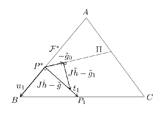
Geometry of $\Pi$ and $\Pi^{*}$ . (See Fig. 8 for an illustration). Assume $\mathrm{dim}(\Pi)>\mathrm{dim}(\Pi^{*})$ (otherwise $\Pi$ is simply equal to $\Pi^{*}$ ). Denote by ${\cal{F}}^{*}$ the face of the probability simplex associated with distributions in ${\mathscr{P}}({\cal{X}}^{*})$ . Fix any $P^{*}\in\Pi^{*}$ and let $u_{1},\cdots,u_{|{\cal{X}}^{*}|-1}$ form a basis for ${\mathscr{L}}({\cal{X}}^{*})$ . Denote by ${\cal{T}}_{0}$ the $|{\mathcal{X}_{\mathrm{cap}}}|-|{\cal{X}}^{*}|$ dimensional subspace of ${\mathscr{L}}({\mathcal{X}_{\mathrm{cap}}})$ that is orthogonal to ${\mathscr{L}}({\cal{X}}^{*})$ , namely,

{\cal{T}}_{0}=\{h\in{\mathscr{L}}({\mathcal{X}_{\mathrm{cap}}}):~h(x)=\mathrm{constant~for~}x\in{\cal{X}}^{*}\}.

The intersection of the affine subspace $P^{*}+{\cal{T}}_{0}$ with ${\mathscr{P}}({\mathcal{X}_{\mathrm{cap}}})$ defines a (scaled) standard simplex ${\cal{S}}\subset{\mathbb{R}}^{|{\mathcal{X}_{\mathrm{cap}}}|-|{\cal{X}}^{*}|+1}$ that has $P^{*}$ as a vertex as well as $|{\mathcal{X}_{\mathrm{cap}}}|-|{\cal{X}}^{*}|$ other vertices denoted by $P_{1},\cdots,P_{|{\mathcal{X}_{\mathrm{cap}}}|-|{\cal{X}}^{*}|}$ . Define $t_{i}=P_{i}-P^{*}\in{\mathscr{L}}({\mathcal{X}_{\mathrm{cap}}})$ for each $i$ . Hence $t_{1},\cdots,t_{|{\mathcal{X}_{\mathrm{cap}}}|-|{\cal{X}}^{*}|}$ form a basis for ${\cal{T}}_{0}$ and are orthogonal to ${\mathscr{L}}({\cal{X}}^{*})$ .

Augmenting ${\cal{T}}$ to include vectors with nonzero mean, we define the following $|{\mathcal{X}_{\mathrm{cap}}}|-|{\cal{X}}^{*}|+1$ dimensional subspace of ${\mathbb{R}}^{\mathcal{X}_{\mathrm{cap}}}$ :

	$\displaystyle{\cal{T}}$	$\displaystyle\triangleq$	$\displaystyle\{z=h+\alpha 1,\;h\in{\cal{T}}_{0},\,\alpha\in{\mathbb{R}}\}$
		$\displaystyle=$	$\displaystyle\{z\in{\mathbb{R}}^{\mathcal{X}_{\mathrm{cap}}}:~z(x)=\mathrm{constant~for~}x\in{\cal{X}}^{*}\}$

and the infinite cones

	$\displaystyle{{\cal{C}}_{{\cal{T}}_{0}}^{\mathrm{in}}}$	$\displaystyle\triangleq$	$\displaystyle\left\{h\in{\cal{T}}_{0}:\;h=\sum_{i}\alpha_{i}t_{i},\;\alpha_{i}\geq 0,\;i=1,2,\cdots,\|{\mathcal{X}_{\mathrm{cap}}}\|-\|{\cal{X}}^{*}\|\right\}$		(4.17)
		$\displaystyle=$	$\displaystyle\{h\in{\mathscr{L}}({\mathcal{X}_{\mathrm{cap}}}):~h(x)=\mathrm{constant~for~}x\in{\cal{X}}^{},\;h(x)\geq 0\;\forall x\in{\mathcal{X}_{\mathrm{cap}}}\setminus{\cal{X}}^{}\}$		(4.17)

and

	$\displaystyle{{\cal{C}}_{\cal{T}}^{\mathrm{out}}}$	$\displaystyle\triangleq$	$\displaystyle\{z\in{\cal{T}}:z^{\top}t_{i}\geq 0,\;i=1,2,\cdots,\|{\mathcal{X}_{\mathrm{cap}}}\|-\|{\cal{X}}^{*}\|\}$		(4.18)
		$\displaystyle=$	$\displaystyle\{z\in{\mathbb{R}}^{\mathcal{X}_{\mathrm{cap}}}:~z(x)=\mathrm{constant~for~}x\in{\cal{X}}^{},\;z(x)\geq 0\;\forall x\in{\mathcal{X}_{\mathrm{cap}}}\setminus{\cal{X}}^{}\}.$		(4.18)

Also define the polytopes

$\displaystyle\mathcal{C}^{\mathrm{in}}$	$\displaystyle\triangleq$	$\displaystyle\left\{h\in{\mathscr{L}}({\mathcal{X}_{\mathrm{cap}}}):\mathrm{Proj}_{{\cal{T}}_{0}}(h)\in{{\cal{C}}_{{\cal{T}}_{0}}^{\mathrm{in}}}\right\}$	(4.19)
	$\displaystyle=$	$\displaystyle\{h\in{\mathscr{L}}({\mathcal{X}_{\mathrm{cap}}}):~h(x)\geq 0\;\forall x\in{\mathcal{X}_{\mathrm{cap}}}\setminus{\cal{X}}^{*}\}$	(4.19)
$\displaystyle\mathcal{C}^{\mathrm{out}}$	$\displaystyle\triangleq$	$\displaystyle\left\{z\in{\mathbb{R}}^{\mathcal{X}_{\mathrm{cap}}}:\mathrm{Proj}_{\cal{T}}(z)\in{{\cal{C}}_{\cal{T}}^{\mathrm{out}}}\right\}$	(4.20)
	$\displaystyle=$	$\displaystyle\{z\in{\mathbb{R}}^{\mathcal{X}_{\mathrm{cap}}}:~z(x)\geq 0\;\forall x\in{\mathcal{X}_{\mathrm{cap}}}\setminus{\cal{X}}^{*}\}.$	(4.20)

Note that $P^{*}+h\in{\mathscr{P}}({\mathcal{X}_{\mathrm{cap}}})\;\Rightarrow\;h\in\mathcal{C}^{\mathrm{in}}$ .

Denote by $\tilde{g}_{0}$ and $\tilde{g}_{1}$ respectively the projections of $\tilde{g}$ of (4.9) onto $\mathrm{ker}({\mathsf{J}_{\mathrm{cap}}})$ and $\mathrm{ker}({\mathsf{J}_{\mathrm{cap}}})^{\perp}$ . By the extremal property of $P^{*}$ in $\Pi$ , we have $-\tilde{g}_{0}^{\top}(P-P^{*})\geq 0$ for all $P\in\Pi$ , hence,

-\tilde{g}_{0}\in\mathcal{C}^{\mathrm{out}}.

(4.21)

The following properties follow immediately from the symmetry properties of the standard simplex.

•

Any $P\in{\mathscr{P}}({\mathcal{X}_{\mathrm{cap}}})$ satisfies $\mathrm{Proj}_{{\cal{T}}_{0}}(P-P^{*})\in{{\cal{C}}_{{\cal{T}}_{0}}^{\mathrm{in}}}$ , i.e., $P-P^{*}\in\mathcal{C}^{\mathrm{in}}$ .

•

For all $z\in{\cal{T}}$ ,

z\in{{\cal{C}}_{\cal{T}}^{\mathrm{out}}}\quad\Longleftrightarrow\quad\mathrm{Proj}_{\mathrm{ker}({\mathsf{J}_{\mathrm{cap}}})}(z)\in\mathcal{C}^{\mathrm{out}}.

(4.22)

•

For all $h\in\mathcal{C}^{\mathrm{in}}$ and $z\in{{\cal{C}}_{\cal{T}}^{\mathrm{out}}}$ ,

$h^{\top}z\geq 0.$ (4.23)

If $\mathrm{dim}(\Pi)=\mathrm{dim}(\Pi^{*})$ , we define $\mathcal{C}^{\mathrm{in}}={\mathscr{L}}({\mathcal{X}_{\mathrm{cap}}})$ .

An optimization game. Now consider the game with payoff function

\Gamma(h,\tilde{h})\triangleq\frac{1}{2}\tilde{h}^{\top}{\mathsf{J}_{\mathrm{cap}}}\tilde{h}+\tilde{h}^{\top}\breve{g}-h^{\top}({\mathsf{J}_{\mathrm{cap}}}\tilde{h}-\tilde{g}),\quad\begin{cases}h,\tilde{h}\in{\mathscr{L}}({\mathcal{X}_{\mathrm{cap}}})&:~r=|{\mathcal{X}_{\mathrm{cap}}}|\\ h\in\mathcal{C}^{\mathrm{in}},\;\tilde{h}\in{\cal{H}}&:~\mathrm{else,}\end{cases}

(4.24)

to be maximized over $h$ and minimized over $\tilde{h}$ . The payoff function is linear in $h$ and convex quadratic in $\tilde{h}$ . Recall ${\cal{H}}={\mathscr{L}}({\cal{X}}^{*})\cap\mathrm{ker}({\mathsf{J}})^{\perp}$ was defined in (2.35).

Lemma 4.25 below shows that the game (4.24) admits a saddlepoint and will be used to prove Prop. 8.9. Fig. 8 provides a geometrical illustration of the saddlepoint property in the case of rank-deficient ${\mathsf{J}_{\mathrm{cap}}}$ .

One might expect that $\inf_{h}\Gamma(h,\tilde{h})=-\infty$ because the payoff function is linear in $h$ . This is true for all $\tilde{h}$ , except for a special choice $\tilde{h}^{*}$ . The key idea in this game is most easily understood in the case $\Pi^{*}$ is a singleton ( ${\mathsf{J}}$ has rank $|{\cal{X}}^{*}|$ ). Then the variable $\tilde{h}\in{\cal{H}}\perp\mathrm{ker}({\mathsf{J}_{\mathrm{cap}}})$ has $r-1\geq|{\cal{X}}^{*}|-1$ degrees of freedom, hence one can construct $\tilde{h}^{*}$ to “cancel” $\tilde{g}$ in the sense that $z={\mathsf{J}_{\mathrm{cap}}}\tilde{h}^{*}-\tilde{g}\in{\cal{T}}$ is orthogonal to ${\mathscr{L}}({\cal{X}}^{*})$ (i.e., $z$ satisfies $|{\cal{X}}^{*}|-1$ orthogonality conditions). Moreover $z\in{{\cal{C}}_{\cal{T}}^{\mathrm{out}}}$ , hence by (4.23), $h^{\top}({\mathsf{J}_{\mathrm{cap}}}\tilde{h}^{*}-\tilde{g})=h^{\top}z\geq 0$ for all $h\in\mathcal{C}^{\mathrm{in}}$ . The argument can be extended to the case $\Pi^{*}$ is not a singleton, by exploiting the fact that $\tilde{g}$ is orthogonal to $\mathrm{ker}({\mathsf{J}})$ .

Lemma 4.5

The game (4.24) admits a saddlepoint $(h^{*},\tilde{h}^{*})$ where $\tilde{h}^{*}={\mathsf{J}}^{+}\tilde{g}$ and $h^{*}={\mathsf{J}}^{+}g\in{\cal{H}}$ . The value of the game is $\Gamma^{*}=\frac{1}{2}\|g\|_{{\mathsf{J}}^{+}}^{2}-\frac{1}{2}\|\breve{g}\|_{{\mathsf{J}}^{+}}^{2}$ , where $g=\tilde{g}+\breve{g}$ . The saddlepoint satisfies the equalizer property

\Gamma(h,\tilde{h}^{*})=\Gamma(h^{*},\tilde{h}^{*})\leq\Gamma(h^{*},\tilde{h})\quad\forall\mathrm{~feasible~}h,\tilde{h}.

(4.25)

Proof. First consider the maximization of $\Gamma(h,\tilde{h})$ with respect to $h$ . We have

\displaystyle\sup_{\mathrm{feasible~}h}\Gamma(h,\tilde{h})

\displaystyle=

\displaystyle\frac{1}{2}\tilde{h}^{\top}{\mathsf{J}_{\mathrm{cap}}}\tilde{h}+\tilde{h}^{\top}\breve{g}-\inf_{\mathrm{feasible~}h}[h^{\top}({\mathsf{J}_{\mathrm{cap}}}\tilde{h}-\tilde{g})]

(4.26)

If $\tilde{h}={\mathsf{J}}^{+}g=\tilde{h}^{*}$ , we claim that the infimum above is zero.

•

If the capacity-achieving input distribution is unique, this is straightforward: ${\cal{X}}^{*}={\mathcal{X}_{\mathrm{cap}}}$ , ${\mathsf{J}_{\mathrm{cap}}}={\mathsf{J}}$ has rank $|{\mathcal{X}_{\mathrm{cap}}}|$ , and ${\mathsf{J}_{\mathrm{cap}}}\tilde{h}^{*}-\tilde{g}$ is equal to the mean of the vector $-\tilde{g}$ times the vector $\mathds{1}\{x\in{\mathcal{X}_{\mathrm{cap}}}\}$ . Since this vector is orthogonal to the feasible space ${\mathscr{L}}({\mathcal{X}_{\mathrm{cap}}})$ for $h$ , the infimum of (4.26) is zero and is achieved by any $h\in{\mathscr{L}}({\mathcal{X}_{\mathrm{cap}}})$ . For any other choice of $\tilde{h}$ , the infimum would be $-\infty$ .

•

If the capacity-achieving input distribution is not unique, then ${\mathsf{J}_{\mathrm{cap}}}$ has rank $r<|{\mathcal{X}_{\mathrm{cap}}}|$ .

–

Case I: $\Pi^{*}$ is a singleton. By (4.14), ${\mathsf{J}}$ has rank $|{\cal{X}}^{*}|$ , and by (4.15), $|{\cal{X}}^{*}|\leq r$ . We have $({\mathsf{J}}\tilde{h}^{*}-\tilde{g})(x)=({\mathsf{J}_{\mathrm{cap}}}\tilde{h}^{*}-\tilde{g})(x)=$ constant for all $x\in{\cal{X}}^{*}$ or equivalently, $z\triangleq{\mathsf{J}_{\mathrm{cap}}}\tilde{h}^{*}-\tilde{g}\perp{\mathscr{L}}({\cal{X}}^{*})$ , hence $z\in{\cal{T}}$ . Moreover $z+\tilde{g}_{0}={\mathsf{J}_{\mathrm{cap}}}\tilde{h}^{*}-\tilde{g}_{1}\perp\mathrm{ker}({\mathsf{J}_{\mathrm{cap}}})$ , hence $\mathrm{Proj}_{\mathrm{ker}({\mathsf{J}_{\mathrm{cap}}})}(z)=-\tilde{g}_{0}$ , hence (4.21) and (4.22) imply $z\in{{\cal{C}}_{\cal{T}}^{\mathrm{out}}}$ . Therefore

\inf_{h\in\mathcal{C}^{\mathrm{in}}}[h^{\top}({\mathsf{J}_{\mathrm{cap}}}\tilde{h}^{*}-\tilde{g})]=\inf_{h\in\mathcal{C}^{\mathrm{in}}}h^{\top}z=0

where the last equality follows from (4.23).

–

Case II: $\mathrm{dim}(\Pi^{*})=k\geq 1$ . We have $z={\mathsf{J}_{\mathrm{cap}}}\tilde{h}^{*}-\tilde{g}\perp\mathrm{ker}({\mathsf{J}_{\mathrm{cap}}})$ . By (4.14), nullity $({\mathsf{J}})=k$ . Let $u_{1},\cdots,u_{k}$ be basis vectors for ${\mathscr{L}}({\cal{X}}^{*})\cap\mathrm{ker}({\mathsf{J}})$ and $u_{k+1},\cdots,u_{|{\cal{X}}^{*}|-1}$ be basis vectors for ${\mathscr{L}}({\cal{X}}^{*})\cap\mathrm{ker}({\mathsf{J}})^{\perp}={\cal{H}}$ . By the extremal property of $\Pi^{*}$ , we have $\tilde{g}^{\top}u_{1}=\cdots=\tilde{g}^{\top}u_{k}=0$ . Since $u_{1},\cdots,u_{k}\in\mathrm{ker}({\mathsf{J}})\subseteq\mathrm{ker}({\mathsf{J}_{\mathrm{cap}}})$ , we obtain $z^{\top}u_{1}=\cdots=z^{\top}u_{k}=0$ . On the other hand, the minimizing variable $\tilde{h}\in{\cal{H}}$ is in the range of ${\mathsf{J}}$ and therefore of ${\mathsf{J}_{\mathrm{cap}}}$ , and has $r-1$ degrees of freedom which can be used to satisfy the $|{\cal{X}}^{*}|-k-1\leq r-1$ equations $z^{\top}u_{k+1}=\cdots=z^{\top}u_{|{\cal{X}}^{*}|-1}=0$ . Therefore choosing $\tilde{h}=\tilde{h}^{*}$ results in $z\perp{\mathscr{L}}({\cal{X}}^{*})$ again, and the rest of the proof follows as in Case I above.

Next, consider the minimization of $\Gamma(h,\tilde{h})$ with respect to $\tilde{h}$ . Fix $h=h^{*}$ . Then

	$\displaystyle\Gamma(h^{*},\tilde{h})$	$\displaystyle=$	$\displaystyle\frac{1}{2}\tilde{h}^{\top}{\mathsf{J}_{\mathrm{cap}}}\tilde{h}-\tilde{h}^{\top}({\mathsf{J}_{\mathrm{cap}}}h^{}-\breve{g})+h^{\top}\tilde{g}$		(4.27)
		$\displaystyle=$	$\displaystyle\frac{1}{2}\tilde{h}^{\top}{\mathsf{J}}\tilde{h}-\tilde{h}^{\top}({\mathsf{J}}h^{}-\breve{g})+h^{\top}\tilde{g}$		(4.27)

which is a convex quadratic function of $\tilde{h}$ . By (2.36), its minimizer is obtained as ${\mathsf{J}}^{+}({\mathsf{J}}h^{*}-\breve{g})={\mathsf{J}}^{+}(g-\breve{g})={\mathsf{J}}^{+}\tilde{g}=\tilde{h}^{*}$ , and the inequality holds in (4.25).

Hence $(h^{*},\tilde{h}^{*})$ is a saddlepoint, and the value of the game is

\Gamma^{*}=\Gamma(h^{*},\tilde{h}^{*})=\frac{1}{2}\tilde{h}^{*\top}{\mathsf{J}}\tilde{h}^{*}+\tilde{h}^{*\top}\breve{g}.

Moreover

\Gamma^{*}=\frac{1}{2}\tilde{g}^{\top}{\mathsf{J}}^{+}(\tilde{g}+2\breve{g})=\frac{1}{2}(g-\breve{g})^{\top}{\mathsf{J}}^{+}(g+\breve{g})=\frac{1}{2}g^{\top}{\mathsf{J}}^{+}g-\frac{1}{2}\breve{g}^{\top}{\mathsf{J}}^{+}\breve{g}.

(4.28)

$\Box$

5 Background: Refined Asymptotics

This section reviews basic techniques for central limit asymptotics and strong large deviations.

5.1 Central Limit Asymptotics

We first review some key results on the asymptotics of a normalized sum of independent random variables. Consider first iid random variables $U_{i},i\geq 1$ , with common cdf $F_{U}$ , finite mean $\mu$ , variance $\sigma^{2}>0$ , and skewness $S\triangleq{\mathbb{E}}[(U-\mu)^{3}]/\sigma^{3/2}$ . The normalized random variable

T_{n}=\frac{\sum_{i=1}^{n}U_{i}-n\mu}{\sqrt{n\sigma^{2}}}

(5.29)

has zero mean and unit variance and by the Central Limit Theorem, converges in distribution to ${\cal{N}}(0,1)$ . Denote by $F_{n}$ the cdf of $T_{n}$ .

iid Nonlattice Random Variables. If $\{U_{i}\}_{i=1}^{\infty}$ are iid nonlattice random variables, the Cramér-Esséen theorem [26, p. 49] [22, p. 538] for nonlattice random variables states that

F_{n}(t)=\Phi(t)-\frac{S}{6\sqrt{n}}(1-t^{2})\,\phi(t)+o(1/\sqrt{n})

(5.30)

uniformly in $t$ , i.e.,

\lim_{n\to\infty}\left\{\sqrt{n}\sup_{t\in{\mathbb{R}}}\left|F_{n}(t)-\Phi(t)-\frac{S}{6\sqrt{n}}(1-t^{2})\,\phi(t)\right|\right\}=0.

The $o(1/\sqrt{n})$ remainder in (5.30) can be strengthened to $O(1/n)$ for strongly nonlattice random variables, i.e., distributions that satisfy Cramér’s condition on the characteristic function $\hat{f}$ of $U$ :

\lim_{|\omega|\to\infty}|\hat{f}(\omega)|<1,

(5.31)

in which case (5.30) is the first-order Edgeworth expansion of $F_{n}$ [21, 24].

Higher-order expansions in terms of successive powers of $n^{-1/2}$ can also be derived [21, 22, 23, 24] but a two-term expansion suffices for our purposes. The Berry-Esséen formula $|F_{n}(t)-\Phi(t)|\leq\frac{A_{3}}{6V^{3/2}\sqrt{n}}$ (where $A_{3}\triangleq{\mathbb{E}}[|U-\mu|^{3}]$ is the absolute third central moment of $U$ ) that was used in [6, 8] does not yield the sharp asymptotics of interest here.

Let $\epsilon=1-\alpha$ and $t_{\epsilon}$ and $t_{\epsilon,n}$ be the upper $\alpha$ -quantiles of $\Phi$ and $F_{n}$ respectively, i.e., $\Phi(t_{\epsilon})=\alpha$ and $F_{n}(t_{\epsilon,n}^{-})\leq\alpha\leq F_{n}(t_{\epsilon,n})$ . The precise asymptotics of $t_{\epsilon,n}$ are of interest, in particular the Cornish-Fisher inversion formula [21, 23, 24, 34] yields

t_{\epsilon,n}=t_{\epsilon}+\frac{S}{6\sqrt{n}}(t_{\epsilon}^{2}-1)+o(n^{-1/2}).

(5.32)

iid Lattice Random Variables. If $\{U_{i}\}_{i=1}^{\infty}$ are iid lattice random variables with span $d$ , the normalized sum $T_{n}$ of (5.29) is also a lattice random variable (with span $d/\sqrt{n\sigma^{2}}$ ) and its cdf $F_{n}(t)$ is piecewise constant with jumps of size $O(n^{-1/2})$ at the lattice points. An $o(n^{-1/2})$ asymptotic approximation to $F_{n}$ can still be constructed, analogously to (5.30) in the nonlattice case [26, pp. 52—67] [22, p. 540]. In particular, (5.30) holds at the midpoints of the lattice. At the lattice points, (5.30) holds with $F_{n}(t)$ replaced with $\frac{1}{2}[F_{n}(t)+F_{n}(t^{-})]$ .

Non-iid Random Variables. In case $U_{i},\,i\geq 1$ , are independent but have different distributions, with respective means $\mu_{i}$ and variances $\sigma_{i}^{2}$ such that

\overline{\sigma}_{n}^{2}\triangleq\frac{1}{n}\sum_{i=1}^{n}\sigma_{i}^{2}

(5.33)

is bounded away from 0 and $\infty$ as $n\to\infty$ , let

\overline{S}_{n}\triangleq\frac{\frac{1}{n}\sum_{i=1}^{n}{\mathbb{E}}[(U_{i}-\mu_{i})^{3}]}{\overline{\sigma}_{n}^{3}}.

(5.34)

Then the expansions (5.30) and (5.32) for the iid nonlattice case hold with $S$ replaced by $\overline{S}_{n}$ [22, pp. 546, 547]: ⁵⁵ 5 Note a typo in [22, Eqn (6.1)], where $s_{n}^{2}$ should be replaced with $s_{n}^{3}$ .

	$\displaystyle F_{n}(t)$	$\displaystyle=$	$\displaystyle\Phi(t)-\frac{\overline{S}_{n}}{6\sqrt{n}}(1-t^{2})\,\phi(t)+o(1/\sqrt{n})$		(5.35)
	$\displaystyle t_{\epsilon,n}$	$\displaystyle=$	$\displaystyle t_{\epsilon}+\frac{\overline{S}_{n}}{6\sqrt{n}}(t_{\epsilon}^{2}-1)+o(n^{-1/2})$		(5.36)

provided that the following additional assumptions hold: each $U_{i}$ has bounded fourth moment, and there exists $\delta>0$ such that

\left|\prod_{i=1}^{n}\hat{f}_{i}(\omega)\right|=o(n^{-1/2})\quad\mathrm{uniformly~in~}\omega>\delta

(5.37)

where $\hat{f}_{i}(\omega)\triangleq{\mathbb{E}}[e^{i\omega U_{i}}]$ is the characteristic function of $U_{i}$ . Condition (5.37) holds when each $U_{i}$ is a nonlattice random variable, as well as in many problems where each $U_{i}$ is a lattice random variable (but $\sum_{i=1}^{n}U_{i}$ is not). In the case each $\sum_{i=1}^{n}U_{i}$ is a lattice random variable with span $d_{n}$ , (5.37) does not hold but the $o(n^{-1/2})$ asymptotic approximation (5.30) to $F_{n}$ holds at midpoints of the lattice, with $\sigma^{2}$ and $S$ replaced with $\overline{\sigma}_{n}^{2}$ and $\overline{S}_{n}$ of (5.33) and (5.34).

5.2 Strong Large-Deviations Asymptotics

Conventional large-deviations methods characterize the exponential decay of tail probabilities, in particular, Cramér’s theorem [25] states that

-\frac{1}{n}\log P^{n}\left\{\sum_{i=1}^{n}U_{i}\geq na\right\}\sim\Lambda(a)\quad\mbox{as~}n\to\infty,\quad\forall a>{\mathbb{E}}[U]

where $U_{i},\,i\geq 1$ is a sequence of iid random variables with common distribution $P$ , cumulant generating function (cgf) $\kappa(s)=\log{\mathbb{E}}_{P}[e^{sU}]$ , and large-deviations function $\Lambda(a)=\sup_{s}[as-\kappa(s)]$ .

Strong large-deviations asymptotics provide arbitrarily accurate approximations to tail probabilities, using Laplace’s method of asymptotic expansion of integrals. If $U$ is a nonlattice random variable and $U_{i},\,i\geq 1$ , are iid then the Bahadur-Rao theorem [20] yields

P^{n}\left\{\sum_{i=1}^{n}U_{i}\geq na\right\}\sim\frac{e^{-n\Lambda(a)}}{s\sqrt{2\pi n\kappa^{\prime\prime}(s)}}\quad\mbox{as~}n\to\infty

(5.38)

where $s$ satisfies $\kappa^{\prime}(s)=a$ . Define the normalized random variable $W_{n}=(\sum_{i=1}^{n}U_{i}-na)/\sqrt{n\kappa^{\prime\prime}(s)}$ which has zero mean and unit variance, and the exponentially tilted distribution $d\tilde{F}_{U}(u)\triangleq e^{su-\kappa(s)}dF_{U}(u)$ . Denote by $\widetilde{F}_{n}$ the cdf for $W_{n}$ when $U$ has cdf $\tilde{F}_{U}$ . The asymptotic formula (5.38) is obtained by writing the identity

P^{n}\left\{\sum_{i=1}^{n}U_{i}\geq na\right\}=e^{-n\Lambda(a)}\int_{0}^{\infty}e^{-s\sqrt{n\kappa^{\prime\prime}(s)}v}d\widetilde{F}_{n}(v)

(5.39)

and evaluating the asymptotics of the integral in the right side. Since $U$ is a nonlattice random variable, $\widetilde{F}_{n}$ does not exhibit $O(n^{-1/2})$ jumps, and (5.38) is derived by applying the Cramér-Esséen expansion (5.30) to $\widetilde{F}_{n}$ .

For lattice random variables, $\widetilde{F}_{n}$ has jumps of size $O(n^{-1/2})$ in the vicinity of the origin. Blackwell and Hodges [19] showed that the right side of (5.38) is multiplied by a bounded, oscillatory function of $n$ . In particular, if $na$ is in the range of the sum $\sum_{i=1}^{n}U_{i}$ , then

P^{n}\left\{\sum_{i=1}^{n}U_{i}\geq na\right\}\sim\frac{d\,e^{-n\Lambda(a)}}{(1-e^{-sd})\sqrt{2\pi n\kappa^{\prime\prime}(s)}}\quad\mbox{as~}n\to\infty

(5.40)

where $d$ is the span of the lattice random variable $U$ . As expected, the asymptotic expansion (5.40) coincides with (5.38) in the limit as $d\to 0$ .

Example: Tail of binomial distribution Bi( $n,p$ ) which is a sum of $n$ iid Be( $p$ ) random variables where $1/2\leq p<1$ . Then $\kappa(s)=\log(1+e^{s})$ and $\kappa^{\prime\prime}(s)=e^{s}/(1+e^{s})^{2}$ . The large-deviations function is $\Lambda(a)=d(a\|p)=a\log\frac{a}{p}+(1-a)\log\frac{1-a}{1-p}$ for $a\in(p,1)$ , and $s$ that achieves the supremum in the definition of $\Lambda(a)$ is $s=\log\frac{a}{1-a}$ , corresponding to $\kappa^{\prime\prime}(s)=a(1-a)$ . The lattice span is $d=1$ . Thus (5.40) yields

\Pr\{\mathrm{Bi}(n,p)\geq na\}\sim\frac{a}{2a-1}\,\frac{e^{-nd(a\|p)}}{\sqrt{2\pi a(1-a)n}},\quad p<a<1,

(5.41)

for any integer $na\to\infty$ . Compare with the oft-used approximation [32, p. 115] which states, for $p=1/2$ ,

\frac{e^{-nd(a\|p)}}{\sqrt{2\pi a(1-a)n}}\leq\Pr\{\mathrm{Bi}(n,p)\geq na\}\leq e^{-nd(a\|p)}.

Clearly the lower bound is tighter than the upper bound as it captures the $n^{-1/2}$ asymptotic term.

A generalization of (5.38) to the non-iid case was given by Bucklew and Sadowsky [31]. An even more more general expression for both the nonlattice and the lattice cases was obtained by Chaganty and Sethuraman [27, Theorems 3.3 and 3.5] in the non-iid case. The following special case is particularly relevant to this paper: evaluate the asymptotics of $\Pr\{Z_{n}\geq na_{n}\}$ where $a_{n}$ is a sequence converging to a limit $a$ , and $Z_{n}$ is a sequence of random variables with respective cdf’s $F_{n}$ and moment generating functions (mgf) $M_{(n)}(s)\triangleq{\mathbb{E}}[e^{sZ_{n}}]$ , assumed to be nonvanishing and analytic in the region $\Omega=\{s\in{\mathbb{C}}~:~|s|<\overline{s}\}$ for some $\overline{s}>0$ . Denote by $n\overline{\kappa}_{n}(s)$ the cgf for $Z_{n}$ , and by

\overline{\Lambda}_{n}(a)=\sup_{s\in{\mathbb{R}}}[as-\overline{\kappa}_{n}(s)]

(5.42)

the associated large-deviations function. Assume the supremum defining $\overline{\Lambda}_{n}(a_{n})$ is achieved at $s_{n}\in\Omega$ , hence $a_{n}=\overline{\kappa}_{n}^{\prime}(s_{n})$ . Define the exponentially tilted distribution $\widetilde{F}_{n}(t)\triangleq\int_{-\infty}^{t}\exp\{s_{n}u-a_{n}\kappa_{n}(s_{n})\}\,dF_{n}(u)$ and the normalized random variable $W_{n}=(\widetilde{Z}_{n}-na_{n})/\sqrt{n\kappa_{n}^{\prime\prime}(s_{n})}$ which has zero mean and unit variance when $\widetilde{Z}_{n}$ has cdf $\widetilde{F}_{n}$ . Denoting by $\widetilde{G}_{n}$ the resulting cdf for $W_{n}$ , one obtains [27, p. 1683]

\Pr\{Z_{n}\geq na_{n}\}=e^{-n\overline{\Lambda}_{n}(a_{n})}\int_{0}^{\infty}e^{-s_{n}\sqrt{n\kappa_{n}^{\prime\prime}(s_{n})}v}d\widetilde{G}_{n}(v).

(5.43)

The characteristic function of $W_{n}$ is obtained from (5.43) as [27, Eqn (3.7)]

\hat{f}_{n}(\omega)=\exp\left\{-\frac{i\omega na_{n}}{\sqrt{n\kappa_{n}^{\prime\prime}(s_{n})}}\right\}\,\frac{M_{(n)}(s_{n}+i\omega/\sqrt{n\kappa_{n}^{\prime\prime}(s_{n})})}{M_{(n)}(s_{n})},\quad\omega\in{\mathbb{R}}

(5.44)

where $i=\sqrt{-1}$ . Further assume there exists $n_{0}\in{\mathbb{N}}$ such that ⁶⁶ 6 It was assumed in [27] that $n_{0}=1$ but this restriction is unnecessary.

(CS1): $\exists\tilde{\kappa}<\infty$ such that $|\kappa_{n}(s)|<\tilde{\kappa}$ for all $n\geq n_{0}$ and $s\in\Omega$ .
(CS2): $\exists V_{0}>0$ such that $\kappa_{n}^{\prime\prime}(s_{n})>V_{0}$ for all $n\geq n_{0}$ .

If $Z_{n}$ is a nonlattice random variable, assume that

(CS3)

$\exists\delta_{0}>0$ such that

\sup_{\delta<|\omega|\leq\lambda s_{n}}\left|\frac{M_{(n)}(s_{n}+i\omega)}{M_{(n)}(s_{n})}\right|=o(1/\sqrt{n})

(5.45)

for any given $\delta$ and $\lambda$ such that $0<\delta<\delta_{0}<\lambda$ .

Under Assumptions (CS1),(CS2),(CS3), $W_{n}$ converges in distribution to ${\cal{N}}(0,1)$ . Theorem 3.3 of [27] in the nonlattice case (with $a_{n}$ , $s_{n}$ , $\overline{\kappa}_{n}$ and $\overline{\Lambda}_{n}$ respectively playing the roles of $m_{n}$ , $\tau_{n}$ , $\psi_{n}$ and $\gamma_{n}$ in [27]) states that analogously to (5.38),

\Pr\left\{Z_{n}\geq na_{n}\right\}\sim\frac{e^{-n\overline{\Lambda}_{n}(a_{n})}}{s_{n}\sqrt{2\pi n\overline{\kappa}_{n}^{\prime\prime}(s_{n})}}\quad\mathrm{as~}n\to\infty.

(5.46)

In the lattice case, let $Z_{n}$ have span $d_{n}$ and $a_{n}$ be in the range of $Z_{n}/n$ . Then $W_{n}$ is lattice-valued with span $d_{n}/\sqrt{n\kappa_{n}^{\prime\prime}(s_{n})}$ and zero offset. Assumption (CS3) above is replaced with

(CS3’)

$\exists\delta_{1}>0$ such that for all $0<\delta<\delta_{1}$ ,

\sup_{\delta<|\omega|\leq\pi/d_{n}}\left|\frac{M_{(n)}(s_{n}+i\omega)}{M_{(n)}(s_{n})}\right|=o(1/\sqrt{n}).

Under Assumptions (CS1),(CS2),(CS3’), Theorem 3.5 of [27] in the lattice case states that analogously to (5.40),

\Pr\left\{Z_{n}\geq na_{n}\right\}\sim\frac{d_{n}\,e^{-n\overline{\Lambda}_{n}(a_{n})}}{(1-e^{-s_{n}d_{n}})\,\sqrt{2\pi n\overline{\kappa}_{n}^{\prime\prime}(s_{n})}}\quad\mathrm{as~}n\to\infty.

(5.47)

Again (5.47) coincides with (5.46) in the limit as $d_{n}\to 0$ . In all cases considered, to obtain sharp asymptotics of the form (5.46) or (5.47), the analysis begins with the identity (5.43), and the key step is to verify the asymptotics of the normalized random variable $W_{n}$ .

6 Strong Large Deviations for Likelihood Ratios

This section presents new results on strong large deviations for likelihood ratios. Of particular interest are NP tests, which are instrumental in deriving the strong converse to the channel coding theorem. The full asymptotics of deterministic NP tests for distributions with iid components were obtained by Strassen [6, Theorem 1, p. 690]. He also derived somewhat looser bounds for the case of distributions with independent but not identically distributed components [6, Theorem 3, p. 702], as did Polyanskiy et al. [8, Lemma 58, p. 2340] allowing randomized tests.

In this section we derive the full asymptotics of such NP tests. The starting point is a strong large-deviations analysis of likelihood ratios (Sec. 6.1), followed by an application to NP testing (Sec. 6.2).

6.1 Likelihood Ratio with Varying Component Distributions

The basic probabilistic model is as follows. Let $Y_{i},\,1\leq i\leq n$ , be independent random variables with respective distributions $P_{i}$ and $Q_{i}$ under hypotheses $H_{1}$ and $H_{0}$ , respectively. Write ${\mathbb{P}}_{n}\triangleq\prod_{i=1}^{n}P_{i}$ and ${\mathbb{Q}}_{n}\triangleq\prod_{i=1}^{n}Q_{i}$ . Assume the following holds:

(LR1)

For each $i\geq 1$ : $P_{i}\ll Q_{i}$ ( $P_{i}$ is dominated by $Q_{i}$ ).

(LR2)

Under $P_{i}$ , the loglikelihood ratio $L_{i}\triangleq\log dP_{i}(Y_{i})/dQ_{i}(Y_{i})$ has finite mean $D_{i}=D(P_{i}\|Q_{i})$ , finite variance $V_{i}=V(P_{i}\|Q_{i})$ , and finite third central moment $T_{i}=T(P_{i}\|Q_{i})$ . Let

\overline{D}_{n}=\frac{1}{n}\sum_{i=1}^{n}D_{i},\quad\overline{V}_{n}=\frac{1}{n}\sum_{i=1}^{n}V_{i},\quad\overline{T}_{n}=\frac{1}{n}\sum_{i=1}^{n}T_{i},\quad\overline{S}_{n}=\frac{\overline{T}_{n}}{[\overline{V}_{n}]^{3/2}}.

(6.1)

There exist $n_{0}\in{\mathbb{N}}$ and $V_{0}>0$ such that $\overline{V}_{n}\geq V_{0}$ for all $n\geq n_{0}$ .

(LR3)

Under $Q_{i}$ , the loglikelihood ratio $L_{i}$ has cgf $\kappa_{i}(s)=\log{\mathbb{E}}_{Q_{i}}[e^{sL_{i}}]=(s-1)D_{s}(P_{i}\|Q_{i})$ . There exists an open neighborhood of $s=1$ in which the averaged cgf $\overline{\kappa}_{n}(s)\triangleq\frac{1}{n}\sum_{i=1}^{n}\kappa_{i}(s)$ is analytic for all $n\geq 1$ .

The lattice case is defined by the condition that $\sum_{i=1}^{n}L_{i}$ is a lattice random variable for all $n\geq 1$ . The strongly nonlattice case could be similarly defined as the case where the Cramér condition (5.31) on the mgf of $\sum_{i=1}^{n}L_{i}$ holds for each $n\geq 1$ . Unfortunately Cramér’s condition is inapplicable to finite alphabets, so we weaken it as follows. The following general definition seems general enough to apply to most problems.

Definition 6.1

(Semistrong nonlattice case.) A sequence $\{L_{i}\}_{i\geq 1}$ of independent random variables with respective marginal distributions $\{\pi_{i}\}_{i\geq 1}$ satisfies the semistrong nonlattice condition if it satisfies at least one of the following three conditions: ⁷⁷ 7 $W_{1}(\cdot,\cdot)$ denotes the first Wasserstein metric (aka earth mover’s distance) between two probability distributions on ${\mathbb{R}}$ , and $\cdot\star\cdot$ denotes the convolution of two distributions on ${\mathbb{R}}$ .

(NL1): $\forall d>0$ , $\exists n_{0}\in{\mathbb{N}}$ , $\delta>0$ such that $\forall n>n_{0}$ : $\displaystyle\min_{1\leq i\leq n}\inf_{P\in{\mathscr{P}}_{\mathrm{lat}}(d)}W_{1}(\pi_{i},P)\geq\delta$ .
(NL2): $\forall d>0$ , $\exists n_{0}\in{\mathbb{N}}$ , $\delta\in(0,1]$ such that $\forall n>n_{0}$ : $\displaystyle\min_{i\in{\cal{I}}_{\delta}}\inf_{P\in{\mathscr{P}}_{\mathrm{lat}}(d)}W_{1}(\pi_{i},P)\geq\delta$ for some subset ${\cal{I}}_{\delta}$ of $\{1,2,\cdots,n\}$ of size $|{\cal{I}}_{\delta}|\geq\delta n$ .
(NL3): $\forall d>0$ , $\exists n_{0}\in{\mathbb{N}}$ , $\delta\in(0,\frac{1}{2}]$ such that $\forall n>n_{0}$ : $\displaystyle\min_{i\in{\cal{I}}_{\delta},j\in{\cal{J}}_{\delta}}\inf_{P\in{\mathscr{P}}_{\mathrm{lat}}(d)}W_{1}(\pi_{i}\star\pi_{j},P)\geq\delta$ for some ${\cal{I}}_{\delta}$ and ${\cal{J}}_{\delta}$ , disjoint subsets of $\{1,2,\cdots,n\}$ of size $\geq\delta n$ each.

Condition (NL1) is stronger than merely requiring that each $L_{i}$ be a nonlattice random variable: no subsequence of $\{\pi_{i}\}$ converges to a lattice distribution under the $W_{1}$ metric. Condition (NL2) is weaker as it allows a fraction ( $1-\delta$ ) of the $\pi_{i}$ ’s to be lattice distributions or converge to a lattice distribution. Condition (NL3) is even weaker as it applies to problems such as the Z channel of Sec. 3.4 where each $L_{i}$ is a lattice random variable but the sum $\log\frac{W_{0}(Y)}{Q_{n}(Y)}+\log\frac{W_{1}(Y)}{Q_{n}(Y)}$ is not. Finally there are somewhat pathological problems (not considered in this paper) which pertain neither to the lattice nor to the semistrong nonlattice case, for instance $\sum_{i=2}^{n}L_{i}$ is a lattice random variable for all $n\geq 2$ but $L_{1}$ is not.

Lemma 6.1

(Second-order Taylor expansion of large-deviations function for loglikelihood ratio.) Consider two probability measures $P$ and $Q$ over a common space and assume that $P$ is dominated by $Q$ ( $P\ll Q$ ). Assume the cgf $\kappa(s)=\log{\mathbb{E}}_{Q}[(\frac{dP}{dQ})^{s}]=(s-1)D_{s}(P\|Q)$ for $L\triangleq\log\frac{dP}{dQ}$ (under $Q$ ) is finite and thrice differentiable in an open neighborhood of $s=1$ . Assume $D=D(P\|Q)$ and $V=V(P\|Q)$ are positive and finite, and $T=T(P\|Q)$ is finite. Then the large-deviations function

\Lambda(a)\triangleq\sup_{s}[as-\kappa(s)]

(6.2)

for $L$ satisfies the Taylor expansion

\Lambda(a)=a+\frac{(a-D)^{2}}{2V}+O((a-D)^{3})\quad\mathrm{as~}a\to D.

(6.3)

Proof: see Appendix D.

Proposition 6.2

Let $t$ and $c\in{\mathbb{R}}$ be arbitrary constants and define the sequence

a_{n}=\overline{D}_{n}-t\sqrt{\frac{\overline{V}_{n}}{n}}+\frac{c}{n}.

(6.4)

Assume (LR1), (LR2), and (LR3) hold.
(i) If $\{L_{i}\}_{i\geq 1}$ is a sequence of random variables of the semistrong nonlattice type, then

\displaystyle{\mathbb{Q}}_{n}\left\{\sum_{i=1}^{n}\log\frac{dP_{i}(Y_{i})}{dQ_{i}(Y_{i})}\geq na_{n}\right\}

\displaystyle=

\displaystyle\frac{\exp\{-na_{n}-\frac{t^{2}}{2}+o(1)\}}{\sqrt{2\pi n\overline{V}_{n}}}.

(6.5)

Moreover (6.5) holds if the inequality “ $\,\geq na_{n}$ ” is replaced with a strict inequality.
(ii) If $\sum_{i=1}^{n}L_{i}$ is a lattice random variable for each $n\geq 1$ , denote by $d_{n}$ its span and by $\Omega_{n}$ its range. Then

\displaystyle{\mathbb{Q}}_{n}\left\{\sum_{i=1}^{n}\log\frac{dP_{i}(Y_{i})}{dQ_{i}(Y_{i})}\geq na_{n}\right\}

\displaystyle=

\displaystyle\frac{d_{n}}{1-e^{-{d_{n}}}}\,\frac{\exp\{-na_{n}-\frac{t^{2}}{2}+o(1)\}}{\sqrt{2\pi n\overline{V}_{n}}},\quad na_{n}\in\Omega_{n}.

(6.6)

In particular, if $d_{n}\to 0$ as $n\to\infty$ , the expressions (6.6) and (6.5) coincide.

Proof: See Appendix E.

6.2 Neyman-Pearson Test

Let $P$ and $Q$ be two probability distributions over a set ${\cal{Z}}$ and consider the Neyman-Pearson test for $P$ versus $Q$ at significance level $\alpha$ . Let $Z=\log\frac{dP}{dQ}$ and denote by $\delta~:~{\cal{Z}}\to[0,1]$ a randomized decision rule returning $\delta(z)=\Pr\{\mathrm{Say}~P|Z=z\},\;z\in{\cal{Z}}$ . The type-II error probability of the NP test at significance level $\alpha$ is denoted by

\beta_{\alpha}(P,Q)=\min_{\delta\,:\,{\mathbb{E}}_{P}[\delta(Z)]\geq\alpha}{\mathbb{E}}_{Q}[\delta(Z)]

(6.7)

and is a convex function of $\alpha$ [35].

The following theorem gives the exact asymptotics of a Neyman-Pearson test between ${\mathbb{P}}_{n}=\prod_{i=1}^{n}P_{i}$ and ${\mathbb{Q}}_{n}=\prod_{i=1}^{n}Q_{i}$ at significance level $\alpha=1-\epsilon$ .

Theorem 6.3

(NP Asymptotics.) Assume (LR1), (LR2), and (LR3) hold. Define

a_{n}\triangleq\overline{D}_{n}-\sqrt{\frac{\overline{V}_{n}}{n}}\,t_{\epsilon}-\frac{1}{6n}\overline{S}_{n}\sqrt{\overline{V}_{n}}(t_{\epsilon}^{2}-1).

(6.8)

(i) In the semistrong nonlattice case,

\beta_{\alpha}({\mathbb{P}}_{n},{\mathbb{Q}}_{n})=\frac{\exp\{-na_{n}-\frac{1}{2}t_{\epsilon}^{2}+o(1)\}}{\sqrt{2\pi\overline{V}_{n}n}}.

(6.9)

Moreover ⁸⁸ 8 The $o(n^{-1/2})$ residual in (6.10) can be strengthened to $O(n^{-1})$ in the strong lattice case where Cramér’s condition is satisfied.

{\mathbb{P}}_{n}\left\{\sum_{i=1}^{n}\log\frac{dP_{i}(Y_{i})}{dQ_{i}(Y_{i})}\geq na_{n}\right\}=\alpha+o(n^{-1/2})\quad\mathrm{as~}n\to\infty.

(6.10)

(ii) In the lattice case,

\beta_{\alpha}({\mathbb{P}}_{n},{\mathbb{Q}}_{n})=\frac{d_{n}\,e^{d_{n}/2}}{1-e^{-d_{n}}}\,\frac{\exp\{-na_{n}-\frac{1}{2}t_{\epsilon}^{2}+o(1)\}}{\sqrt{2\pi\overline{V}_{n}n}}

(6.11)

for all $n,\alpha$ such that $na_{n}+\frac{d_{n}}{2}\in\Omega_{n}$ . The function $\beta_{\alpha}({\mathbb{P}}_{n},{\mathbb{Q}}_{n})$ is piecewise linear in $\alpha$ , with breaks at the points satisfying $na_{n}+\frac{d_{n}}{2}\in\Omega_{n}$ . If $d_{n}\to 0$ as $n\to\infty$ , the asymptotic expressions (6.9) and (6.11) coincide.

Proof. The type-II error probability $\beta_{\alpha}({\mathbb{P}}_{n},{\mathbb{Q}}_{n})$ of the NP test is achieved by a randomized likelihood ratio test (LRT) with test statistic $Z_{n}\triangleq\sum_{i=1}^{n}\log\frac{dP_{i}(Y_{i})}{dQ_{i}(Y_{i})}$ [35]:

\delta_{\textrm{NP}}({\mathbf{Y}})=\left\{\begin{array}[]{ll}1&:~Z_{n}>nb_{n}\\ \rho_{n}&:~Z_{n}=nb_{n}\\ 0&:~Z_{n}<nb_{n}\end{array}\right.

where the threshold $nb_{n}$ and randomization parameter $\rho_{n}$ are chosen to satisfy the constraint

\alpha={\mathbb{E}}_{{\mathbb{P}}_{n}}[\delta_{\textrm{NP}}({\mathbf{Y}})]={\mathbb{P}}_{n}\{Z_{n}>nb_{n}\}+\rho_{n}{\mathbb{P}}_{n}\{Z_{n}=nb_{n}\}

(6.12)

hence

{\mathbb{P}}_{n}\{Z_{n}>nb_{n}\}\leq\alpha\leq{\mathbb{P}}_{n}\{Z_{n}\geq nb_{n}\}.

(6.13)

The type-II error probability of the NP test is

\beta_{\alpha}({\mathbb{P}}_{n},{\mathbb{Q}}_{n})={\mathbb{E}}_{{\mathbb{Q}}_{n}}[\delta_{\textrm{NP}}({\mathbf{Y}})]={\mathbb{Q}}_{n}\{Z_{n}\geq nb_{n}\}-(1-\rho_{n}){\mathbb{Q}}_{n}\{Z_{n}=nb_{n}\}

(6.14)

hence satisfies the following lower and upper bounds:

{\mathbb{Q}}_{n}\{Z_{n}>nb_{n}\}\leq\beta_{\alpha}({\mathbb{P}}_{n},{\mathbb{Q}}_{n})\leq{\mathbb{Q}}_{n}\{Z_{n}\geq nb_{n}\}.

(6.15)

By (6.1), we have ${\mathbb{E}}_{{\mathbb{P}}_{n}}[Z_{n}]=n\overline{D}_{n}$ and ${\mathrm{Var}}_{{\mathbb{P}}_{n}}[Z_{n}]=n\overline{V}_{n}$ . Denote by $F_{n}$ the cdf of the normalized random variable

T_{n}\triangleq\frac{Z_{n}-n\overline{D}_{n}}{\sqrt{n\overline{V}_{n}}}.

By (6.13) and the definition of the quantile $t_{\epsilon,n}$ above (5.32), we have

t_{\epsilon,n}=\frac{nb_{n}-n\overline{D}_{n}}{\sqrt{n\overline{V}_{n}}}.

(6.16)

(i) Semistrong nonlattice case. If the cdf $F_{n}$ is continuous at $b_{n}$ , then ${\mathbb{P}}_{n}\{Z_{n}=nb_{n}\}=0$ , and so from (6.12) we have $F_{n}(t_{\epsilon,n})=\alpha$ . Else $F_{n}$ may have a jump of size $o(n^{-1/2})$ . Then ${\mathbb{P}}_{n}\{Z_{n}=nb_{n}\}=o(n^{-1/2})$ and $F_{n}(t_{\epsilon,n})=\alpha+o(n^{-1/2})$ . Applying successively (5.36) and (6.8), we have

	$\displaystyle t_{\epsilon,n}$	$\displaystyle=$	$\displaystyle t_{\epsilon}+\frac{\overline{S}_{n}}{6\sqrt{n}}(t_{\epsilon}^{2}-1)+o(n^{-1/2})$		(6.17)
		$\displaystyle=$	$\displaystyle\frac{na_{n}-n\overline{D}_{n}}{\sqrt{n\overline{V}_{n}}}+o(n^{-1/2}).$		(6.17)

Comparing with (6.16), we obtain $nb_{n}=na_{n}+o(1)$ .

Applying Prop. 6.2(i) with $t=t_{\epsilon}$ and $c=-\frac{1}{6}\overline{S}_{n}\sqrt{\overline{V}_{n}}(t_{\epsilon}^{2}-1)$ , we obtain

{\mathbb{Q}}_{n}\{Z_{n}\geq nb_{n}\}={\mathbb{Q}}_{n}\{Z_{n}\geq na_{n}+o(1)\}=\frac{\exp\{-na_{n}-\frac{1}{2}t_{\epsilon}^{2}+o(1)\}}{\sqrt{2\pi\overline{V}_{n}n}}

and the same asymptotics hold for ${\mathbb{Q}}_{n}\{Z_{n}>nb_{n}\}$ . The claim then follows from (6.15).

(ii) In the lattice case, $\beta_{\alpha}({\mathbb{P}}_{n},{\mathbb{Q}}_{n})$ , viewed as a function of $\alpha$ , is convex and piecewise linear, with breaks at the points where randomization is not needed ( $\rho_{n}=1$ ). At any such point $\alpha$ we have $\beta_{\alpha}({\mathbb{P}}_{n},{\mathbb{Q}}_{n})={\mathbb{Q}}_{n}\{Z_{n}\geq nb_{n}\}$ and $\alpha={\mathbb{P}}_{n}\{Z_{n}\geq nb_{n}\}$ . Recalling the central limit asymptotics for non-iid lattice random variables at the end of Sec. 5.1, (6.17) holds if $na_{n}$ is a midpoint of the lattice, i.e., $na_{n}+\frac{1}{2}d_{n}\in\Omega_{n}$ . Hence $na_{n}=nb_{n}-\frac{1}{2}d_{n}$ , ${\mathbb{P}}_{n}\{Z_{n}\geq na_{n}\}=\alpha+o(n^{-1/2})$ , and by Prop. 6.2(ii),

	$\displaystyle{\mathbb{Q}}_{n}\{Z_{n}\geq nb_{n}\}$	$\displaystyle=$	$\displaystyle\frac{d_{n}}{1-e^{-d_{n}}}\,\frac{\exp\{-nb_{n}-\frac{1}{2}t_{\epsilon}^{2}+o(1)\}}{\sqrt{2\pi\overline{V}_{n}n}}$
		$\displaystyle=$	$\displaystyle\frac{d_{n}\,e^{d_{n}/2}}{1-e^{-d_{n}}}\,\frac{\exp\{-na_{n}-\frac{1}{2}t_{\epsilon}^{2}+o(1)\}}{\sqrt{2\pi\overline{V}_{n}n}}.$

$\Box$

Remark 6.1

Theorem 6.3(i) reduces to Theorem 1 of Strassen [6, p. 690] in the case of iid components and deterministic rules. For the non-iid case, Strassen [6, Theorem 3, p. 702] used the Berry-Esséen theorem to show

|\log\beta_{\alpha}({\mathbb{P}}_{n},{\mathbb{Q}}_{n})+n\overline{D}_{n}-\sqrt{n\overline{V}_{n}}\,t_{\epsilon}+\frac{1}{2}\log n|<\frac{140}{\delta^{8}}

(6.18)

where $\delta$ is any number satisfying the four inequalities

0<\delta<1-\alpha,\quad\sqrt{n}\geq\frac{140}{\delta^{8}},\quad\delta\leq\sqrt{\overline{V}_{n}},\quad\delta\leq\overline{T}_{n}^{-1/3}.

The right side of (6.18) is at least equal to $140/(1-\alpha)^{8}$ , and the inequality holds for $n$ at least equal to $140^{2}/(1-\alpha)^{16}$ .

Remark 6.2

Polyanskiy et al. [9, Lemma 14, p. 33] derived

	$\displaystyle-n\overline{D}_{n}-\sqrt{n\overline{V}_{n}}\,\Phi^{-1}\left(\alpha-\frac{6\overline{S}_{n}+\delta}{\sqrt{n}}\right)+\log\delta-\frac{1}{2}\log n\leq\log\beta_{\alpha}({\mathbb{P}}_{n},{\mathbb{Q}}_{n})$				(6.19)
		$\displaystyle\leq$	$\displaystyle-n\overline{D}_{n}-\sqrt{n\overline{V}_{n}}\,\Phi^{-1}\left(\alpha-\frac{6\overline{S}_{n}}{\sqrt{n}}\right)-\frac{1}{2}\log n+\log\left(\frac{2\log 2}{\sqrt{2\pi\overline{V}_{n}}}+24\overline{S}_{n}\right)$		(6.19)

valid for any $\delta>0$ . (A looser upper bound, without the $\frac{1}{2}\log n$ , is given in [8, Lemma 58, p. 2340]). The lower bound is asymptotic to

-n\overline{D}_{n}-\sqrt{n\overline{V}_{n}}\,\Phi^{-1}(\alpha)-\frac{1}{2}\log n-c_{\alpha}\sqrt{\overline{V}_{n}}(6\overline{S}_{n}+\delta)+\log\delta+o(1)

where $c_{\alpha}>0$ is the derivative of the function $-\Phi^{-1}$ at $\alpha$ . Maximizing this expression over $\delta$ , one obtains $\delta=1/(c_{\alpha}\sqrt{\overline{V}_{n}})$ hence the asymptotic lower bound

\log\beta_{\alpha}({\mathbb{P}}_{n},{\mathbb{Q}}_{n})\geq-n\overline{D}_{n}-\sqrt{n\overline{V}_{n}}\,\Phi^{-1}(\alpha)-\frac{1}{2}\log n-\log\left(c_{\alpha}\sqrt{\overline{V}_{n}}\right)-6c_{\alpha}\sqrt{\overline{V}_{n}}\overline{S}_{n}-1+o(1).

(6.20)

Remark 6.3

Using Chebyshev’s inequality, Polyanskiy et al. [8, Lemma 59, p. 2341] also derived the following nonasymptotic lower bound:

\displaystyle\log\beta_{\alpha}({\mathbb{P}}_{n},{\mathbb{Q}}_{n})\geq-n\overline{D}_{n}-\sqrt{\frac{2n\overline{V}_{n}}{1-\epsilon}}+\log\frac{1-\epsilon}{2}.

(6.21)

A closely related inequality was derived by Kemperman [7, Theorem 7.1].

7 Achievability

The direct coding theorem 3.1 is proved using iid random codes and ML decoding.

Fix $P^{*}$ achieving the maximum in (). From (2.4), (2.9), and (2.25), we define $V_{\mathrm{u}}\triangleq V_{\mathrm{u}}(P^{*},W)$ , $S_{\mathrm{u}}\triangleq S_{\mathrm{u}}(P^{*},W)$ and $\rho\triangleq\rho(P^{*},W)$ . The function

\omega(h,t)\triangleq-\frac{1}{2}\|h\|_{{\mathsf{J}}^{+}}^{2}-\frac{t}{2\sqrt{V_{\mathrm{u}}}}h^{\top}\nabla V_{\mathrm{u}}(P^{*}),\quad h\in{\mathscr{L}}({\cal{X}}),\,t\in{\mathbb{R}}

(7.1)

is quadratic in $h$ and linear in $t$ . It follows from (2.48) and $\sum_{x\in{\cal{X}}}h(x)=0$ that

h^{\top}\nabla V_{\mathrm{u}}(P^{*})=h^{\top}\nabla V(P^{*}).

(7.2)

Recall that $V_{\mathrm{u}}=V_{\epsilon}>0$ by (A1) and that $S_{\mathrm{u}}=S$ . In the remainder of this section, the subscript “u” could be dropped everywhere.

Fixing $t=t_{\epsilon}$ . Recalling (2.36), (2.37), and (2.42), we have

\sup_{h\in{\cal{H}}}\omega(h,t_{\epsilon})=\frac{t_{\epsilon}^{2}}{8V_{\mathrm{u}}}\|\nabla V_{\mathrm{u}}(P^{*})\|_{{\mathsf{J}}^{+}}^{2}=\frac{t_{\epsilon}^{2}}{8}A_{\mathrm{ns}}^{(P^{*})}

(7.3)

where the supremum is achieved at

h^{*}\triangleq-\frac{t_{\epsilon}}{2\sqrt{V_{\epsilon}}}\,{\mathsf{J}}^{+}v^{(P^{*})}\quad\in{\cal{H}}.

(7.4)

Next, define

\hat{t}_{\epsilon,n}\triangleq t_{\epsilon}+\frac{S_{\mathrm{u}}}{6\sqrt{n}}(t_{\epsilon}^{2}-1).

(7.5)

Fix any $h\in{\cal{H}}$ and draw random codes iid from

P_{n}=P^{*}+n^{-1/2}h\quad\in{\mathscr{P}}({\cal{X}}).

(7.6)

Shannon’s codes are obtained as a special case with $h=0$ , but our achievability bound will be obtained when $h=h^{*}$ . The number of codewords is $M_{n}=\lfloor e^{nR_{n}}\rfloor$ where

$\displaystyle nR_{n}$	$\displaystyle=$	$\displaystyle nC-\sqrt{nV_{\mathrm{u}}}\,t_{\epsilon}+\frac{1}{2}\log n+\underline{A}_{\epsilon}+\omega(h,t_{\epsilon})-\frac{t_{\epsilon}^{2}}{8}A_{\mathrm{ns}}^{(P^{*})}$	(7.7)
	$\displaystyle=$	$\displaystyle nC-\sqrt{nV_{\mathrm{u}}}\,t_{\epsilon}+\frac{1}{2}\log n$
		$\displaystyle\quad-\frac{1}{6}S_{\mathrm{u}}\sqrt{V_{\mathrm{u}}}(t_{\epsilon}^{2}-1)+\frac{t_{\epsilon}^{2}}{2}\frac{1-\rho}{1+\rho}+\frac{1}{2}\log(2\pi(1-\rho^{2})V_{\mathrm{u}})+\omega(h,t_{\epsilon})-1$

where the last equality follows from the definition of $\underline{A}_{\epsilon}$ in ().

Random coding scheme. The codeword symbols $\{X_{i}(m),\,1\leq i\leq n,\,1\leq m\leq M_{n}\}$ are drawn iid from the distribution $P_{n}$ of (7.6). Define the random variables

Z_{m,n}\triangleq\log\frac{W^{n}({\mathbf{Y}}|{\mathbf{X}}(m))}{(P_{n}W)^{n}({\mathbf{Y}})}=\sum_{i=1}^{n}\log\frac{W(Y_{i}|X_{i}(m))}{(P_{n}W)(Y_{i})},\quad 1\leq m\leq M_{n}.

(7.8)

Hence $Z_{m,n}$ is the same as the information density $i({\mathbf{X}}(m);{\mathbf{Y}})$ . The ML decoding rule is deterministic and can be written as

\hat{m}=\arg\max_{1\leq m\leq M_{n}}Z_{m,n}.

(7.9)

In case of a tie, an error is declared. ⁹⁹ 9 Decoding performance could potentially be improved using randomization for tie breaking [14].

Overview of error probability analysis. By symmetry of the codebook construction and the decoding rule, the conditional error probability (given message $m$ ) is independent of $m$ . We show that the average error probability over the random ensemble is $\epsilon+o(n^{-1/2})$ , hence there exists a deterministic code with at most the same average error probability. This proves the claim, since by Taylor’s formula, $\sqrt{nV_{\epsilon}}Q^{-1}(\epsilon+o(n^{-1/2}))=\sqrt{nV_{\epsilon}}Q^{-1}(\epsilon)+o(1)$ .

For the calculation below, we assume without loss of generality that $m=1$ was sent. We start from a standard random coding union bound ¹⁰¹⁰ 10 This first step is ubiquitous in analyses of random codes and has also been used in particular to state the RCU bound of [8, Theorem 16].

$\displaystyle\Pr\{\mathrm{Error}\}$	$\displaystyle=$	$\displaystyle\Pr\left\{\max_{m\geq 2}Z_{m,n}\geq Z_{1,n}\right\}$	(7.10)
	$\displaystyle\leq$	$\displaystyle\Pr\left\{Z_{1,n}\leq z_{n}^{}\right\}+\Pr\left\{\max_{m\geq 2}Z_{m,n}\geq Z_{1,n}\geq z_{n}^{}\right\}$
	$\displaystyle\leq$	$\displaystyle\Pr\left\{Z_{1,n}\leq z_{n}^{}\right\}+(M_{n}-1)\Pr\left\{Z_{2,n}\geq Z_{1,n}\geq z_{n}^{}\right\}.$

In the last line, $z_{n}^{*}$ is arbitrary but will be chosen so that the second probability is $\frac{\phi(t_{\epsilon})}{\sqrt{nV_{\mathrm{u}}}}[1+o(1)]$ . We then use precise asymptotics for the two probabilities of (7.10) to derive the desired result.

Thus (7.10) upperbounds the error probability as the sum of two terms. The first is the probability that the correct message scores below some threshold $z_{n}^{*}$ , and the second upperbounds the probability that some incorrect message scores at least as well as the correct message, conditioned on the score of the latter being at least equal to $z_{n}^{*}$ . There is a somewhat weak but possibly significant dependency (via ${\mathbf{Y}}$ ) between the score of an incorrect message and that of the correct message. As shown in the derivations below, this dependency is quantified by the correlation coefficient $\rho$ and contributes to the $O(1)$ term in the achievable rate.

Central Limit Asymptotics of $Z_{1,n}$ . For each $m=1,2,\cdots,M_{n}$ , the pairs $(X_{i}(m),Y_{i})$ , $1\leq i\leq n$ are iid, hence $Z_{m,n}$ is the sum of conditionally (given $m$ ) iid random variables. The mean of $Z_{1,n}$ is given by

{\mathbb{E}}[Z_{1,n}]=n{\mathbb{E}}_{P_{n}\times W}\left[\log\frac{W(Y|X)}{(P_{n}W)(Y)}\right]=nI(P_{n};W).

By (B.1) and (7.6) we have

	$\displaystyle\overline{D}_{n}=I(P_{n};W)$	$\displaystyle=$	$\displaystyle I(P^{};W)-\frac{1}{2}\\|P^{}-P_{n}\\|_{\mathsf{J}}^{2}+o(1/n)$		(7.11)
		$\displaystyle=$	$\displaystyle C-\frac{1}{2n}\\|h\\|_{\mathsf{J}}^{2}+o(1/n).$		(7.11)

The variance of $Z_{1,n}$ is equal to $n$ times the unconditional information variance

\overline{V}_{n}=V_{\mathrm{u}}(P_{n};W)=V_{\mathrm{u}}+\frac{1}{\sqrt{n}}h^{\top}\nabla V_{\mathrm{u}}(P^{*})+o(n^{-1/2})

where the last equality follows from (B.2) and (7.6). Since $V_{\mathrm{u}}>0$ , we obtain

\sqrt{\overline{V}_{n}}=\sqrt{V_{\mathrm{u}}}+\frac{1}{2\sqrt{nV_{\mathrm{u}}}}h^{\top}\nabla V_{\mathrm{u}}(P^{*})+o(n^{-1/2}).

(7.12)

Combining (7.1), (7.11), and (7.12) we obtain

n\overline{D}_{n}-\sqrt{n\overline{V}_{n}}\,t=nC-\sqrt{nV_{\mathrm{u}}}\,t+\omega(h,t)+o(1),\quad\forall t\in{\mathbb{R}}.

(7.13)

The skewness of $Z_{1,n}$ is equal to

\overline{S}_{n}=S_{\mathrm{u}}(P_{n};W)=S_{\mathrm{u}}+O(n^{-1/2}).

(7.14)

Define the normalized random variable

T_{n}\triangleq-\frac{Z_{1,n}-n\overline{D}_{n}}{\sqrt{n\overline{V}_{n}}}

(7.15)

which has zero mean and unit variance and by the Central Limit Theorem, converges in distribution to ${\cal{N}}(0,1)$ . By the Cornish-Fisher inversion formula (5.32), $\hat{t}_{\epsilon,n}$ of (7.5) satisfies

F_{T_{n}}(\hat{t}_{\epsilon,n})=1-\epsilon+o(n^{-1/2}).

(7.16)

Now fix $z_{n}^{*}=n\overline{D}_{n}-\sqrt{n\overline{V}_{n}}\,t_{n}^{*}$ where ¹¹¹¹ 11 To obtain the best $O(1)$ term, we could choose $t_{n}^{*}=\hat{t}_{\epsilon,n}+a/\sqrt{nV_{\mathrm{u}}}$ and optimize $a$ . The optimal choice of $a$ turns out to be 1, hence the choice of (7.17).

t_{n}^{*}\triangleq\hat{t}_{\epsilon,n}+\frac{1}{\sqrt{nV_{\mathrm{u}}}}=t_{\epsilon}+\frac{1}{\sqrt{n}}\left(\frac{S_{\mathrm{u}}}{6}(t_{\epsilon}^{2}-1)+\frac{1}{\sqrt{V_{\mathrm{u}}}}\right).

(7.17)

Hence

z_{n}^{*}=nC-\sqrt{nV_{\mathrm{u}}}\,t_{\epsilon}-\frac{S_{\mathrm{u}}\sqrt{V_{\mathrm{u}}}}{6}(t_{\epsilon}^{2}-1)+\omega(h,t_{\epsilon})-1.

(7.18)

We have

$\displaystyle P_{Z_{1,n}}\{Z_{1,n}<z_{n}^{*}\}$	$\displaystyle\stackrel{{\scriptstyle(a)}}{{=}}$	$\displaystyle\int_{t>t_{n}^{*}}dP_{T_{n}}(t)$	(7.19)
	$\displaystyle=$	$\displaystyle 1-F_{T_{n}}(t_{n}^{*})$
	$\displaystyle\stackrel{{\scriptstyle(b)}}{{=}}$	$\displaystyle 1-F_{T_{n}}(\hat{t}_{\epsilon,n})-(t_{n}^{*}-\hat{t}_{\epsilon,n})\phi(t_{\epsilon})+o(n^{-1/2})$
	$\displaystyle\stackrel{{\scriptstyle(c)}}{{=}}$	$\displaystyle\epsilon-\frac{\phi(t_{\epsilon})}{\sqrt{nV_{\mathrm{u}}}}+o(n^{-1/2})\quad\mathrm{as~}n\to\infty$

where (a), (b), and (c) follow from (7.15), (7.17), and (7.16), respectively.

Large Deviations for $Z_{2,n}$ . The random variables $Z_{m,n},\,m\geq 2,\,n\geq 1$ are identically distributed and are conditionally independent given ${\mathbf{Y}}$ . By (7.8), for $m\geq 2$ , the joint distribution of $(Z_{m,n},Z_{1,n})$ is the same as that of $(\sum_{i=1}^{n}L_{i}^{\prime},\sum_{i=1}^{n}L_{i})$ where

L_{i}^{\prime}\triangleq\log\frac{W(Y_{i}|X_{i}^{\prime})}{(P_{n}W)(Y_{i})},\quad L_{i}\triangleq\log\frac{W(Y_{i}|X_{i})}{(P_{n}W)(Y_{i})},\quad 1\leq i\leq n

are iid with joint distribution $P_{L^{\prime}L}$ induced by $P_{X^{\prime}XY}(x^{\prime},x,y)\triangleq P_{n}(x^{\prime})P_{n}(x)W(y|x)$ .

Denote by $\tilde{P}_{L^{\prime}L}$ the tilted distribution

d\tilde{P}_{L^{\prime}L}(l^{\prime},l)\triangleq e^{l^{\prime}}\,dP_{L^{\prime}L}(l^{\prime},l)

(7.20)

induced by

\tilde{P}_{X^{\prime}XY}(x^{\prime},x,y)=\frac{W(y|x^{\prime})}{(P_{n}W)(y)}P_{X^{\prime}XY}(x^{\prime},x,y)=\frac{P_{n}(x^{\prime})W(y|x^{\prime})W(y|x)P_{n}(x)}{(P_{n}W)(y)}.

(7.21)

The marginals $\tilde{P}_{L^{\prime}}$ and $\tilde{P}_{L}$ are identical with mean ${\mathbb{E}}_{\tilde{P}}[L]={\mathbb{E}}_{\tilde{P}}[L^{\prime}]=\overline{D}_{n}$ and variance ${\mathrm{Var}}_{\tilde{P}}[L]={\mathrm{Var}}_{\tilde{P}}[L^{\prime}]=\overline{V}_{n}$ . Since $X\to Y\to X^{\prime}$ forms a Markov chain under $\tilde{P}$ , we have

{\mathbb{E}}_{\tilde{P}}[L^{\prime}L]={\mathbb{E}}_{(P_{n}W)}\left\{{\mathbb{E}}[L^{\prime}|Y]\,{\mathbb{E}}[L|Y]\right\}={\mathbb{E}}_{(P_{n}W)}{\mathbb{E}}^{2}[i(X;Y)|Y].

Hence ${\mathrm{Cov}}_{\tilde{P}}(L^{\prime},L)={\mathbb{E}}_{(P_{n}W)}{\mathrm{Var}}[i(X;Y)|Y]=V^{r}(P_{n};W)$ , and $\rho_{n}(P;W)=1-V^{r}(P_{n};W)/\overline{V}_{n}$ is the normalized correlation coefficient between $L^{\prime}$ and $L$ under $\tilde{P}$ . Hence $(L^{\prime},L)$ has covariance matrix ${\mathrm{Cov}}_{\tilde{P}}(L,L^{\prime})^{\top}=\overline{V}_{n}\begin{bmatrix}1&\rho_{n}\\ \rho_{n}&1\end{bmatrix}$ where $\overline{V}_{n}=V_{\mathrm{u}}+O(n^{-1/2})$ and $\rho_{n}=\rho+O(n^{-1/2})$ .

Define the normalized random variables

W_{n}^{\prime}\triangleq\frac{\sum_{i=1}^{n}L_{i}^{\prime}-n\overline{D}_{n}}{\sqrt{n\overline{V}_{n}}}+t_{n}^{*}\quad\mathrm{and}\quad W_{n}\triangleq\frac{\sum_{i=1}^{n}L_{i}-n\overline{D}_{n}}{\sqrt{n\overline{V}_{n}}}+t_{n}^{*}.

(7.22)

Hence the second probability in the right side of (7.10) is

	$\displaystyle\Pr\left\{Z_{2,n}\geq Z_{1,n}\geq z_{n}^{*}\right\}$	$\displaystyle=$	$\displaystyle P_{L^{\prime}L}^{n}\left\{\sum_{i=1}^{n}L_{i}^{\prime}\geq\sum_{i=1}^{n}L_{i}\geq n\overline{D}_{n}-\sqrt{n\overline{V}_{n}}t_{n}^{*}\right\}$		(7.23)
		$\displaystyle=$	$\displaystyle P_{L^{\prime}L}^{n}\{0\leq W_{n}\leq W_{n}^{\prime}\}$		(7.23)

Under the tilted distribution $\tilde{P}_{L^{\prime}L}^{n}$ , the random variables $W_{n}^{\prime}$ and $W_{n}$ have means equal to $t$ , unit variance, and correlation coefficient $\rho_{n}$ . Denote their joint cdf by $F_{n}$ and the two-dimensional Gaussian cdf with the same mean and covariance by $\Phi_{t_{n}^{*},\rho_{n}}$ . Recall that $t_{n}^{*}=t_{\epsilon}+O(n^{-1/2})$ and $\rho_{n}=\rho+O(n^{-1/2})$ , and denote the pdf associated with $\Phi_{t_{\epsilon},\rho}$ by $\phi_{t_{\epsilon},\rho}$ . Since the pairs $\{(L_{i}^{\prime},L_{i}),\,1\leq i\leq n\}$ are iid, by the Central Limit Theorem, $F_{n}$ converges pointwise to $\Phi_{t_{\epsilon},\rho}$ . More precisely, analogously to (5.30), the following expansion holds [23, Sec. 6.3]:

F_{n}(w^{\prime},w)=\Phi_{t_{n}^{*},\rho_{n}}(w^{\prime},w)+\frac{1}{\sqrt{n}}f(w^{\prime},w)\,\phi_{t_{n}^{*},\rho_{n}}(w^{\prime},w)+o(n^{-1/2})

(7.24)

where convergence is uniform over ${\mathbb{R}}^{2}$ , and $f(w^{\prime},w)$ is a polynomial function of degree 3.

We have

$\displaystyle P_{L^{\prime}L}^{n}\{0\leq W_{n}\leq W_{n}^{\prime}\}$	$\displaystyle=$	$\displaystyle\int_{{\mathbb{R}}^{n}\times{\mathbb{R}}^{n}}dP_{L^{\prime}L}^{n}({\mathbf{l}}^{\prime},{\mathbf{l}})\,\mathds{1}\left\{0\leq W_{n}\leq W_{n}^{\prime}\right\}$	(7.25)
	$\displaystyle\stackrel{{\scriptstyle(a)}}{{=}}$	$\displaystyle e^{-z_{n}^{}}\,\int_{{\mathbb{R}}^{n}\times{\mathbb{R}}^{n}}d\tilde{P}_{L^{\prime}L}^{n}({\mathbf{l}}^{\prime},{\mathbf{l}})e^{-\left[\sum_{i=1}^{n}l_{i}^{\prime}-z_{n}^{}\right]}\,\mathds{1}\left\{0\leq W_{n}\leq W_{n}^{\prime}\right\}$
	$\displaystyle\stackrel{{\scriptstyle(b)}}{{=}}$	$\displaystyle e^{-z_{n}^{*}}\iint_{0\leq w\leq w^{\prime}}dF_{n}(w^{\prime},w)\,e^{-\sqrt{n\overline{V}_{n}}\,w^{\prime}}$
	$\displaystyle\stackrel{{\scriptstyle(c)}}{{=}}$	$\displaystyle e^{-z_{n}^{*}}\sqrt{n\overline{V}_{n}}\int_{w=0}^{\infty}dF_{n}(w)\int_{w^{\prime}=w}^{\infty}(F_{n}(w^{\prime}\|w)-F_{n}(w\|w))\,e^{-\sqrt{n\overline{V}_{n}}\,w^{\prime}}\,dw^{\prime}$

where (a) follows from (7.20), (b) from (7.22), and (c) is obtained using integration by parts for $w^{\prime}$ . Applying (7.24) yields, after the same algebra as in [20] [36, pp. 110—112]

$\displaystyle P_{L^{\prime}L}^{n}\{0\leq W_{n}\leq W_{n}^{\prime}\}$	$\displaystyle\sim$	$\displaystyle e^{-z_{n}^{*}}\sqrt{nV_{\mathrm{u}}}\iint_{0\leq w\leq w^{\prime}}(\Phi_{t_{\epsilon},\rho}(w^{\prime},w)-\Phi_{t_{\epsilon},\rho}(w,w))\,e^{-\sqrt{n\overline{V}_{n}}\,w^{\prime}}\,dwdw^{\prime}$	(7.27)
	$\displaystyle=$	$\displaystyle\frac{e^{-z_{n}^{*}}}{\sqrt{nV_{\mathrm{u}}}}\int_{u\geq 0}\int_{u^{\prime}\geq u}\left[\Phi_{t_{\epsilon},\rho}\left(\frac{u^{\prime}}{\sqrt{nV_{\mathrm{u}}}},\frac{u}{\sqrt{nV_{\mathrm{u}}}}\right)-\Phi_{t_{\epsilon},\rho}\left(\frac{u}{\sqrt{nV_{\mathrm{u}}}},\frac{u}{\sqrt{nV_{\mathrm{u}}}}\right)\right]\,e^{-u^{\prime}}\,dudu^{\prime}$
	$\displaystyle\sim$	$\displaystyle\frac{e^{-z_{n}^{*}}}{\sqrt{nV_{\mathrm{u}}}}\int_{u\geq 0}\int_{u^{\prime}\geq u}\frac{u^{\prime}-u}{\sqrt{nV_{\mathrm{u}}}}\,\phi_{t_{\epsilon},\rho}\left(\frac{u}{\sqrt{nV_{\mathrm{u}}}},\frac{u}{\sqrt{nV_{\mathrm{u}}}}\right)\,e^{-u^{\prime}}\,dudu^{\prime}$
	$\displaystyle=$	$\displaystyle\frac{e^{-z_{n}^{*}}}{nV_{\mathrm{u}}}\int_{u\geq 0}\,\phi_{t_{\epsilon},\rho}\left(\frac{u}{\sqrt{nV_{\mathrm{u}}}},\frac{u}{\sqrt{nV_{\mathrm{u}}}}\right)\,e^{-u}\,du$
	$\displaystyle\sim$	$\displaystyle\frac{e^{-z_{n}^{*}}}{nV_{\mathrm{u}}}\phi_{t_{\epsilon},\rho}(0,0)$
	$\displaystyle=$	$\displaystyle\frac{e^{-z_{n}^{*}}}{nV_{\mathrm{u}}}\frac{\phi(t_{\epsilon})\exp\{-\frac{1-\rho}{2(1+\rho)}t_{\epsilon}^{2}\}}{\sqrt{2\pi(1-\rho^{2})}}.$

Hence the second term in the right side of (7.10) is

$\displaystyle(M_{n}-1)P_{L^{\prime}L}^{n}\{0\leq W_{n}\leq W_{n}^{\prime}\}$			(7.28)
	$\displaystyle=$	$\displaystyle\frac{\phi(t_{\epsilon})}{\sqrt{nV_{\mathrm{u}}}}\,\exp\left\{nR_{n}-z_{n}^{*}-\frac{1-\rho}{2(1+\rho)}t_{\epsilon}^{2}-\frac{1}{2}\log(2\pi(1-\rho^{2})nV_{\mathrm{u}})+o(1)\right\}$
	$\displaystyle=$	$\displaystyle\frac{\phi(t_{\epsilon})}{\sqrt{nV_{\mathrm{u}}}}[1+o(1)]$

where the last equality follows from (7.7) and (7.18)

Substituting (7.28) and (7.19) into (7.10), we obtain

	$\displaystyle\Pr\{\mathrm{Error}\}$	$\displaystyle\leq$	$\displaystyle\epsilon-\frac{\phi(t_{\epsilon})}{\sqrt{nV_{\mathrm{u}}}}+\frac{\phi(t_{\epsilon})}{\sqrt{nV_{\mathrm{u}}}}+o(n^{-1/2})$
		$\displaystyle=$	$\displaystyle\epsilon+o(n^{-1/2})$

which proves the claim. $\Box$

8 Converse

To prove Theorem 3.2, we begin in Sec. 8.1 with some background from Polyanskiy et al. [8]. Sec 8.2 presents a converse for constant-composition codes under both the maximum and average error probability criteria. Sec 8.3 presents a converse for general codes under the maximum error probability criterion, and Sec 8.4 presents the converse under the average error probability criterion. Each section builds on the results from the previous section.

8.1 Background

Here we review upper bounds on $M_{\mathrm{avg}}^{*}(n,\epsilon)$ and $M_{\max}^{*}(n,\epsilon)$ that are expressed in terms of the type-II error probability of NP tests at significance level $\alpha=1-\epsilon$ .

Theorem 8.1

[8, Theorem 31 p. 2319] The volume $M_{\sf F}$ of any code with codewords in ${\sf F}\subseteq{\cal{X}}^{n}$ and maximum error probability $\epsilon$ satisfies

M_{\sf F}\leq\inf_{Q_{\mathbf{Y}}}\sup_{{\mathbf{x}}\in\sf F}\frac{1}{\beta_{1-\epsilon}(W^{n}(\cdot|{\mathbf{x}}),Q_{{\mathbf{Y}}})}

(8.1)

where the supremum is over all feasible codewords, and the infimum is over all probability distributions on ${\cal{Y}}^{n}$ .

Theorem 8.2

[8, Theorem 27 p. 2318] The volume $M_{\sf F}$ of any code with codewords in ${\sf F}\subseteq{\cal{X}}^{n}$ and average error probability $\epsilon$ satisfies

M_{\sf F}\leq\sup_{P_{\mathbf{X}}}\inf_{Q_{\mathbf{Y}}}\frac{1}{\beta_{1-\epsilon}(P_{{\mathbf{X}}}\times W^{n},P_{{\mathbf{X}}}\times Q_{{\mathbf{Y}}})}

(8.2)

where the supremum is over all probability distributions on $\sf F$ , and the infimum is over all probability distributions on ${\cal{Y}}^{n}$ .

It was later shown that the order of sup and inf can be exchanged in (8.2) [37]; this property is unrelated to the saddlepoint property of Prop. 8.9 presented later in this section.

In some cases $\beta_{1-\epsilon}(P_{{\mathbf{Y}}|{\mathbf{X}}={\mathbf{x}}},Q_{{\mathbf{Y}}})$ is constant for all ${\mathbf{x}}\in{\sf F}$ , e.g., when $Q_{\mathbf{Y}}=Q_{Y}^{n}$ is the $n$ -fold product of a distribution $Q_{Y}$ over ${\cal{Y}}$ , and when all ${\mathbf{x}}\in{\sf F}$ have the same composition. With some abuse of notation, we write $\beta_{1-\epsilon}(Q_{Y}^{n})=\beta_{1-\epsilon}(P_{{\mathbf{Y}}|{\mathbf{X}}={\mathbf{x}}},Q_{Y}^{n})$ . Then the following result holds.

Theorem 8.3

[8, Theorem 28 p. 2318]. Fix a distribution $Q_{Y}$ over ${\cal{Y}}$ and assume $\beta_{1-\epsilon}(P_{{\mathbf{Y}}|{\mathbf{X}}={\mathbf{x}}},Q_{Y}^{n})$ $=\beta_{1-\epsilon}(Q_{Y}^{n})$ for each ${\mathbf{x}}\in{\sf F}\subseteq{\cal{X}}^{n}$ . Then the volume $M_{\sf F}$ of any code with codewords in ${\sf F}\subseteq{\cal{X}}^{n}$ and average error probability $\epsilon$ satisfies $M_{\sf F}\leq 1/\beta_{1-\epsilon}(Q_{Y}^{n})$ .

This result was used in Polyanskiy et al. [8] to derive a converse theorem for constant-composition codes. Denote by $M_{\mathrm{cc}}^{*}(n,\epsilon)$ the maximal number of codewords for any constant-composition code over the DMC $W$ , with maximal error probability $\epsilon$ .

Theorem 8.4

[8, Theorem 48 p. 2331]. If $0<\epsilon\leq 1/2$ , there exists $n_{0}\in{\mathbb{N}}$ and a constant $F>0$ such that

\forall n>n_{0}:\quad\log M_{\mathrm{cc}}^{*}(n,\epsilon)\leq nC-\sqrt{nV_{\epsilon}}t_{\epsilon}+\frac{1}{2}\log n+F.

The key idea in the proof of this theorem (Eqn (494) p. 2350) is to use a result on the asymptotics of NP tests (Lemma 58 p. 2340) that provides a lower bound on $\beta_{1-\epsilon}(Q_{Y}^{n})$ .

Finally, applying [8, Eqn (284) p. 2332]

M_{\max}^{*}(n,\epsilon)\leq M_{\mathrm{avg}}^{*}(n,\epsilon)\leq\frac{\tau}{\tau-1}M_{\max}^{*}(n,\tau\epsilon)

with $\tau=1+1/\sqrt{n}$ , we obtain ${\cal{Q}}^{-1}(\tau\epsilon)={\cal{Q}}^{-1}(\epsilon)+O(n^{-1/2})$ . Hence $M_{\max}^{*}(n,\tau\epsilon)$ and $M_{\max}^{*}(n,\epsilon)$ asymptotically differ only by a constant and

M_{\max}^{*}(n,\epsilon)\leq M_{\mathrm{avg}}^{*}(n,\epsilon)\leq\sqrt{n}\,[M_{\max}^{*}(n,\epsilon)+O(1)].

(8.3)

Hence the gap between the maximum log-volumes under the average and maximum error probability criteria is at most $\frac{1+o(1)}{2}\log n$ .

8.2 Converse for Constant-Composition Codes

Fix some positive vanishing sequence $\delta_{n}$ . Consider $Q=(\tilde{P}W)$ where $\tilde{P}\in{\mathscr{P}}({\cal{X}})$ and define

\hat{\zeta}_{n}(P,Q;\delta_{n})\triangleq\left\{\begin{array}[]{l}nD(W\|Q|P)-\sqrt{nV(W\|Q|P)}\,t_{\epsilon}+F_{\epsilon}(W\|Q|P)\\ \quad\mathrm{if~}\exists P_{0}\in\Pi:~\|P-P_{0}\|_{\infty}\leq\delta_{n},\,\|\tilde{P}-P_{0}\|_{\infty}\leq\delta_{n},\\ nD(W\|Q|P)+\sqrt{\frac{2nV(W\|Q|P)}{1-\epsilon}}-\log\frac{1-\epsilon}{2}\\ \quad\mathrm{else.}\end{array}\right.

(8.4)

For $Q=(PW)$ this function is equal to

\hat{\zeta}_{n}(P;W;\delta_{n})\triangleq\left\{\begin{array}[]{ll}nI(P;W)-\sqrt{nV(P;W)}t_{\epsilon}+F_{\epsilon}(P;W)&\mathrm{if~}\exists P_{0}\in\Pi:~\|P-P_{0}\|_{\infty}\leq\delta_{n}\\ nI(P;W)+\sqrt{\frac{2nV(P;W)}{1-\epsilon}}-\log\frac{1-\epsilon}{2}&\mathrm{else.}\end{array}\right.

(8.5)

In the case $\epsilon>\frac{1}{2}$ , note that $\sqrt{\frac{2nV(P;W)}{1-\epsilon}}\leq-\frac{1}{2}\sqrt{nV_{\max}}t_{\epsilon}$ for all $P\in\Pi$ .

Proposition 8.5

Assume (A1) and (A3) hold. Fix any positive vanishing sequence $\delta_{n}$ . Consider any sequence ${\mathbf{x}}\in{\cal{X}}^{n}$ and any distribution $\tilde{P}\in{\mathscr{P}}({\cal{X}})$ such that $\tilde{P}\in\Pi(\delta_{n})$ if $\hat{P}_{\mathbf{x}}\in\Pi(\delta_{n})$ (and $\tilde{P}$ is unrestricted otherwise). Let $Q=(\tilde{P}W)$ . The following asymptotic inequality holds uniformly over ${\mathbf{x}}$ and $Q$ satisfying the conditions above:

-\log\beta_{1-\epsilon}(W^{n}(\cdot|{\mathbf{x}}),Q^{n})\leq\hat{\zeta}_{n}(\hat{P}_{\mathbf{x}},Q;\delta_{n})+\frac{1}{2}\log n+o(1).

(8.6)

Proof. Define

$\displaystyle\overline{D}_{n}$	$\displaystyle\triangleq$	$\displaystyle\frac{1}{n}\sum_{i=1}^{n}D(W_{x_{i}}\\|Q)=\sum_{x\in{\cal{X}}}P(x)D(W_{x}\\|Q)=D(W\\|Q\|P),$	(8.7)
$\displaystyle\overline{V}_{n}$	$\displaystyle\triangleq$	$\displaystyle\frac{1}{n}\sum_{i=1}^{n}V(W_{x_{i}}\\|Q)=\sum_{x\in{\cal{X}}}P(x)V(W_{x}\\|Q)=V(W\\|Q\|P),$	(8.8)
$\displaystyle\overline{T}_{n}$	$\displaystyle\triangleq$	$\displaystyle\frac{1}{n}\sum_{i=1}^{n}T(W_{x_{i}}\\|Q)=\sum_{x\in{\cal{X}}}P(x)T(W_{x}\\|Q)=T(W\\|Q\|P),$	(8.9)
$\displaystyle\overline{S}_{n}$	$\displaystyle\triangleq$	$\displaystyle\frac{\overline{T}_{n}}{[\overline{V}_{n}]^{3/2}}$	(8.10)

and

na_{n}\triangleq n\overline{D}_{n}-\sqrt{n\overline{V}_{n}}t_{\epsilon}-\frac{1}{6}\overline{S}_{n}\sqrt{\overline{V}_{n}}(t_{\epsilon}^{2}-1).

Similarly $\frac{1}{n}\sum_{i=1}^{n}D_{s}(W_{x_{i}}\|Q)=D_{s}(W\|Q|P)$ .

Case I: $P=\hat{P}_{\mathbf{x}}\in\Pi(\delta_{n})$ and $\tilde{P}\in\Pi(\delta_{n})$ . Then (2.13) and (8.4) yield $\hat{\zeta}_{n}(P,Q;\delta_{n})=\zeta_{n}(P,Q)$ where $Q=(\tilde{P}W)$ . Assumption (LR1) of Sec. 6.1 holds because $\mathrm{supp}\{Q^{*}\}={\cal{Y}}$ , hence $\mathrm{supp}\{(\tilde{P}W)\}={\cal{Y}}$ for all $\tilde{P}\in\Pi(\delta_{n})$ , and $n$ large enough. Assumption (LR2) holds because ${\cal{X}}$ is finite, $V_{\min}=\min_{P\in\Pi}V(P;W)>0$ by (A1), and $V(W_{x}\|\cdot)$ is continuous at $Q^{*}$ , hence $\overline{V}_{n}=V(W\|Q|P)>\frac{1}{2}V_{\min}$ for all $P,\tilde{P}\in\Pi(\delta_{n})$ , $Q=(\tilde{P}W)$ , and $n$ large enough. Assumption (LR3) holds because ${\cal{X}}$ and ${\cal{Y}}$ are finite alphabets.

First assume $Q$ is such that $L=\log\frac{W(Y|X)}{Q(Y)}$ is a nonlattice random variable. Then the sequence of loglikelihoods $L_{i}\triangleq\log[W(Y_{i}|x_{i})/Q(Y_{i})],\,i\geq 1$ satisfies the semistrong nonlattice condition (Def. 6.1), where the marginal distribution $\pi_{i}$ is a function of $x_{i}$ . Further note that $\{L_{i}\}$ satisfies a stronger property in which the statements after the semicolons in (NL1)—(NL3) hold not only $\forall n>n_{0}$ but also $\forall{\mathbf{x}}$ such that $\hat{P}_{\mathbf{x}}\in\Pi(\delta_{n})$ . The Taylor expansions of Lemma 4.3 (with $P=\hat{P}_{\mathbf{x}}$ ) and (E.1) (with ${\mathbb{P}}_{n}=W^{n}(\cdot|{\mathbf{x}})$ ) hold uniformly over ${\mathbf{x}}$ such that $\hat{P}_{\mathbf{x}}\in\Pi(\delta_{n})$ . The asymptotics of $\beta_{1-\epsilon}(W^{n}(\cdot|{\mathbf{x}}),Q^{n})$ are then obtained from Theorem 6.3(i):

$\displaystyle-\log\beta_{1-\epsilon}(W^{n}(\cdot\|{\mathbf{x}}),Q^{n})$			(8.11)
	$\displaystyle=$	$\displaystyle na_{n}+\frac{1}{2}\log n+\frac{1}{2}t_{\epsilon}^{2}+\frac{1}{2}\log(2\pi\overline{V}_{n})+o(1)$
	$\displaystyle=$	$\displaystyle nD(W\\|Q\|P)-\sqrt{nV(W\\|Q\|P)}\,t_{\epsilon}+\frac{1}{2}\log n+F_{\epsilon}(W\\|Q\|P)+o(1)$
	$\displaystyle=$	$\displaystyle\zeta_{n}(P,Q)+\frac{1}{2}\log n+o(1)$

uniformly over $\hat{P}_{\mathbf{x}},\tilde{P}\in\Pi(\delta_{n})$ .

The case where $Q$ is such that $L$ is a lattice random variable with span $d_{n}$ yields the same solution (8.11) because under (A3), $d_{n}$ must tend to 0 as $n\to\infty$ . Indeed our condition on $Q$ may be written as $Q=Q^{*}+(\tilde{h}W)$ where $\|\tilde{h}\|_{\infty}\leq 1$ . Hence

L=L_{0}-\log\left(1+\delta_{n}\frac{(\tilde{h}W)(Y)}{Q^{*}(Y)}\right)

where $L_{0}=\log\frac{W(Y|X)}{Q^{*}(Y)}$ is a nonlattice random variable, and $\frac{(\tilde{h}W)(Y)}{Q^{*}(Y)}$ is bounded. Hence $L=L_{0}+O(\delta_{n})$ with probability 1, and $d_{n}\to 0$ . The asymptotics of $\beta_{1-\epsilon}(W^{n}(\cdot|{\mathbf{x}}),Q^{n})$ are then obtained from Theorem 6.3(ii), and (8.11) holds again. Thus (8.6) holds as well.

Case II: $\tilde{P}\notin\Pi(\delta_{n})$ or $\hat{P}_{\mathbf{x}}\notin\Pi(\delta_{n})$ . We use the nonasymptotic bound of (6.21) with ${\mathbb{P}}_{n}=W^{n}(\cdot|{\mathbf{x}})$ and ${\mathbb{Q}}_{n}=Q^{n}$ :

$\displaystyle-\log\beta_{1-\epsilon}(W^{n}(\cdot\|{\mathbf{x}}),Q^{n})$	$\displaystyle\leq$	$\displaystyle n\overline{D}_{n}+\sqrt{\frac{2n\overline{V}_{n}}{1-\epsilon}}-\log\frac{1-\epsilon}{2}$	(8.12)
	$\displaystyle=$	$\displaystyle nD(W\\|Q\|P)+\sqrt{\frac{2nV(W\\|Q\|P)}{1-\epsilon}}-\log\frac{1-\epsilon}{2}$
	$\displaystyle=$	$\displaystyle\hat{\zeta}_{n}(P,Q;\delta_{n})$

and therefore (8.6) holds again. $\Box$

Theorem 8.6

Assume (A1) and (A3) hold.

(i) The volume $M[P]$ of any code of constant composition $P\in{\mathscr{P}}_{n}({\cal{X}})$ and (maximum or average) error probability $\epsilon$ satisfies

\log M[P]\leq\hat{\zeta}_{n}(P;W;\delta_{n})+\frac{1}{2}\log n+o(1)

(8.13)

uniformly over $P$ , for any positive vanishing sequence $\delta_{n}$ . There exist constants $c_{1},c_{2}>0$ such that the following statements hold.

(ii) (Bad Types). If $\delta_{n}\gg n^{-1/4}$ , there exists $n_{0}\geq 1$ such that

\log M[P]\leq nC-c_{2}n\delta_{n}^{2}\quad\forall P\notin\Pi(\delta_{n}),\;n\geq n_{0}.

(8.14)

(iii) (Mediocre Types). If $\delta_{n}\gg n^{-1/2}\log n$ and $P\notin\Pi^{*}(\delta_{n})$ then

\log M[P]\leq nC-\sqrt{nV_{\epsilon}}\,t_{\epsilon}-c_{1}\sqrt{n}\delta_{n}[1+o(1)].

(8.15)

(iv) (All Types).¹²¹² 12 The result (8.16) is not used in this paper but is stated for completeness.

\log M[P]\leq nC-\sqrt{nV_{\epsilon}}\,t_{\epsilon}+\frac{1}{2}\log n+\overline{A}_{\epsilon}+o(1).

(8.16)

Proof. (i) Fix the distributions $Q=(PW)$ and $Q_{\mathbf{Y}}=Q^{n}$ , and any positive vanishing sequence $\delta_{n}$ . Then $\hat{\zeta}_{n}(P,Q;\delta_{n})=\hat{\zeta}_{n}(P;W;\delta_{n})$ . Under the maximum-error probability criterion, (8.13) follows from Theorem 8.1 and Prop. 8.6. Since $\beta_{1-\epsilon}(W^{n}(\cdot|{\mathbf{x}}),Q^{n})$ is the same for all ${\mathbf{x}}$ of composition $P$ , (8.13) also holds under the average-error probability criterion [8, Lemma 29 p. 2318].

(ii) If $\delta_{n}\gg n^{-1/4}$ and $P\notin\Pi(\delta_{n})$ , the Taylor expansion (B.1) implies that $I(P;W)\leq C-2c_{2}\delta_{n}^{2}$ $\forall n\geq n_{1}$ for some $c_{2}>0$ and $n_{1}\geq 1$ . Let $\overline{V}\triangleq\max_{P\in{\mathscr{P}}({\cal{X}})}V(P;W)$ which is finite. Then (8.13) and (8.5) yield

$\displaystyle\log M[P]$	$\displaystyle\leq$	$\displaystyle nI(P;W)+\sqrt{\frac{2nV(P;W)}{1-\epsilon}}-\log\frac{1-\epsilon}{2}$
	$\displaystyle\leq$	$\displaystyle nC-2c_{2}\delta_{n}^{2}+\sqrt{\frac{2n\overline{V}}{1-\epsilon}}-\log\frac{1-\epsilon}{2}$
	$\displaystyle\leq$	$\displaystyle nC-c_{2}n\delta_{n}^{2}\quad\forall n>n_{0},\,P\notin\Pi(\delta_{n})$

for some $n_{0}\geq n_{1}$ . This establishes (8.14).

(iii) If $P\notin\Pi(n^{-1/5})$ , the claim follows directly from Part (ii). If $n^{-1/2}\log n\ll\delta_{n}<n^{-1/5}$ and $P\in\Pi(n^{-1/5})\setminus\Pi^{*}(\delta_{n})$ , then applying successively (8.13), (8.5), and Lemma 4.2(iii) with $\epsilon_{n}=n^{-1/5}$ , we obtain

	$\displaystyle\log M[P]\leq\hat{\zeta}_{n}(P;W;\epsilon_{n})+\frac{1}{2}\log n+o(1)$	$\displaystyle=$	$\displaystyle\zeta_{n}(P;W)+\frac{1}{2}\log n+o(1)$
		$\displaystyle\leq$	$\displaystyle nC-\sqrt{nV_{\epsilon}}\,t_{\epsilon}-c_{1}\sqrt{n}\delta_{n}[1+o(1)],$

hence (8.15) holds.

(iv) If $P\notin\Pi^{*}(n^{-1/2}\log n)$ , the claim follows directly from Part (iii). For $P\in\Pi^{*}(n^{-1/2}\log n)$ , the claim follows from (8.30) which is proved in the next section. $\Box$

8.3 Converse for General Codes, Maximum Error Probability Criterion

In this section we derive an upper bound on the volume of arbitrary codes with maximum error probability $\epsilon$ .

Theorem 8.7

Assume (A1) and (A3) hold. The volume $M_{{\cal{X}}^{n}}$ of any code with codewords in ${\cal{X}}^{n}$ and maximum error probability $\epsilon\in(0,1)$ satisfies

\log M_{{\cal{X}}^{n}}\leq nC-\sqrt{nV_{\epsilon}}t_{\epsilon}+\frac{1}{2}\log n+\overline{A}_{\epsilon}+o(1).

(8.17)

The theorem is proved at the end of this section. The analysis involves an optimization over ${\mathscr{P}}({\cal{X}})$ . A different treatment is needed for a “good set” ${\mathscr{P}}_{1}$ of distributions that are close to $\Pi^{*}$ and for the complement set ${\mathscr{P}}_{1}^{c}$ .

First we provide some motivation for the method of proof and give some definitions and two propositions (8.18 and 8.9). Fix any ${\sf F}\subseteq{\cal{X}}^{n}$ and let ${\mathscr{P}}_{0}$ be any subset of ${\mathscr{P}}({\cal{X}})$ such that ${\mathbf{x}}\in{\sf F}\,\Rightarrow\,\hat{P}_{\mathbf{x}}\in{\mathscr{P}}_{0}$ . Let ${\cal{Q}}\triangleq\{Q=(PW),\,P\in{\mathscr{P}}({\cal{X}})\}$ . The following proposition follows immediately from Theorem 8.1 and Prop. 8.6.

Proposition 8.8

Assume (A1) and (A3) hold. Fix any positive vanishing sequence $\delta_{n}$ , and consider any subset ${\mathscr{P}}_{0}$ (possibly dependent of $n$ ) of ${\mathscr{P}}({\cal{X}})$ . The volume $M[{\mathscr{P}}_{0}]$ of any code with codewords of composition $\in{\mathscr{P}}_{0}$ and maximum error probability $\epsilon\in(0,1)$ satisfies

\log M[{\mathscr{P}}_{0}]\leq\inf_{Q\in{\cal{Q}}}\sup_{P\in{\mathscr{P}}_{0}}\hat{\zeta}_{n}(P,Q;\delta_{n})+\frac{1}{2}\log n+o(1).

(8.18)

At first sight this suggests seeking a solution to the minmax game with payoff function $\hat{\zeta}_{n}(P,Q;\delta_{n})$ over ${\mathscr{P}}_{0}\times{\mathscr{P}}({\cal{Y}})$ .

If $\Pi\subset{\mathscr{P}}_{0}$ , a version of the above game with payoff

\lim_{n\to\infty}\frac{1}{n}\zeta_{n}(P,Q)=D(W\|Q|P)=\sum_{x\in{\cal{X}}}P(x)D(W_{x}\|Q)

admits the well-known equalizer saddlepoint solution $(P,Q)=(P^{*},Q^{*})$ for each $P^{*}\in\Pi$ [33], as given in Lemma 4.1(i). Owing to the equalizer property in (4.2), we have

\displaystyle\inf_{Q\in{\cal{Q}}}\sup_{P\in{\mathscr{P}}_{0}}D(W\|Q|P)

\displaystyle=

\displaystyle\sup_{P\in{\mathscr{P}}_{0}}\inf_{Q\in{\cal{Q}}}D(W\|Q|P)=C

even if ${\mathscr{P}}_{0}$ is not a convex set.

For finite $n$ there is generally no saddlepoint because unlike $D(W\|Q|P)$ , the payoff function $\zeta_{n}(P,Q)$ of (2.13) is not linear nor even concave in $P$ for $\epsilon<\frac{1}{2}$ due to the $O(\sqrt{n})$ variance term. However

•

In the CT weakly symmetric case where $\Pi^{*}=\{P^{*}\}$ (singleton), $V(W_{x}\|Q^{*})=V(P^{*};W)$ and $F_{\epsilon}(W_{x}\|Q^{*})=F_{\epsilon}(P^{*};W)$ for all $x\in{\cal{X}}$ , the capacity-achieving input and output distributions $P^{*}$ and $Q^{*}$ are uniform. The game clearly admits an asymptotic saddlepoint solution $(P,Q)=(P^{*},Q^{*})$ in the sense that

\zeta_{n}(P,Q^{*})+o(1)\leq\zeta_{n}(P^{*},Q^{*})\leq\zeta_{n}(P^{*},Q)+o(1)\quad\forall P\in{\mathscr{P}}({\cal{X}}),\,\forall Q\in{\cal{Q}},

(8.19)

and the asymptotic value of the game is $\zeta_{n}(P^{*},Q^{*})=\zeta_{n}(P^{*};W)$ .

•

In the nonsymmetric case with $\Pi^{*}=\{P^{\prime}\}$ (singleton), using Taylor expansion of $\zeta_{n}(\cdot,\cdot)$ around $(P^{\prime},Q^{*})$ (Lemmas 4.3 and 4.25), we shall see there still exists an asymptotic saddlepoint $(P_{n}^{\prime},\tilde{Q}_{n}^{*})$ if the maximization over $P$ is restricted to a vanishing neighborhood of $P^{\prime}$ , of size $\delta_{n}=\frac{1}{n^{1/4}\log n}$ :

\zeta_{n}(P,\tilde{Q}_{n}^{*})+o(1)\leq\zeta_{n}(P_{n}^{\prime},\tilde{Q}_{n}^{*})\leq\zeta_{n}(P_{n}^{\prime},Q),\quad\forall P:\,\|P-P^{\prime}\|\leq\delta_{n},\,\forall Q.

(8.20)

The asymptotic value of the game is $\zeta_{n}(P_{n}^{\prime},\tilde{Q}_{n}^{*})=nC-\sqrt{nV_{\epsilon}}\,t_{\epsilon}+\overline{A}_{\epsilon}+o(1)$ , and the asymptotic saddlepoint is given in (8.25), (8.26).

•

If $\Pi^{*}$ is not a singleton, the saddlepoint property (8.20) holds for each $P^{\prime}\in\Pi^{*}$ , $\tilde{Q}_{n}^{*}$ is independent of $P^{\prime}$ , and $\zeta_{n}(P_{n}^{\prime},\tilde{Q}_{n}^{*})\leq nC-\sqrt{nV_{\epsilon}}\,t_{\epsilon}+\overline{A}_{\epsilon}+o(1)$ . The upper bound is achieved when $P^{\prime}$ is the maximizer of (3.1).

Instead of applying Theorem 8.1 with ${\sf F}={\cal{X}}^{n}$ directly, we define a set of subcodes with maximum error probability $\epsilon$ each, and derive the asymptotics for these subcodes. The upper bound on $M$ is the sum of the upper bounds on the volume of the subcodes.

Define the “good” class of codewords

{\sf F}_{1}\triangleq\left\{{\mathbf{x}}\in{\cal{X}}^{n}~:~\hat{P}_{\mathbf{x}}\in\Pi^{*}\left(\frac{1}{n^{1/4}\log n}\right)\right\}

(8.21)

and the corresponding “good” class of distributions over ${\cal{X}}$

{\mathscr{P}}_{1}\triangleq\Pi^{*}\left(\frac{1}{n^{1/4}\log n}\right).

(8.22)

Hence ${\mathbf{x}}\in{\sf F}_{1}\,\Leftrightarrow\,\hat{P}_{\mathbf{x}}\in{\mathscr{P}}_{1}$ .

The following proposition shows that for each $P^{\prime}\in\Pi^{*}$ , the payoff function $\zeta_{n}(P,\tilde{Q}_{n}^{*})$ is constant (up to a vanishing term) over the neighborhood $\{P\in{\mathscr{P}}({\cal{X}}):\,\|P-P^{\prime}\|_{\infty}\leq\frac{1}{n^{1/4}\log n}\}$ . Define the two correction vectors

	$\displaystyle h^{\prime}$	$\displaystyle\triangleq$	$\displaystyle-\frac{t_{\epsilon}}{2\sqrt{V_{\epsilon}}}\,{\mathsf{J}}^{+}v^{(P^{\prime})}\quad\in{\cal{H}}$		(8.23)
	$\displaystyle\tilde{h}^{*}$	$\displaystyle\triangleq$	$\displaystyle-\frac{t_{\epsilon}}{2\sqrt{V_{\epsilon}}}\,{\mathsf{J}}^{+}\tilde{v}\qquad\in{\cal{H}}$		(8.24)

to which we associate modifications $P_{n}^{\prime}$ and $\tilde{Q}_{n}^{*}$ of the capacity-achieving input and output distributions as follows:

	$\displaystyle P_{n}^{\prime}$	$\displaystyle\triangleq$	$\displaystyle P^{\prime}+n^{-1/2}h^{\prime}\qquad\quad\;\;\;\;\in{\mathscr{P}}({\cal{X}})$		(8.25)
	$\displaystyle\tilde{Q}_{n}^{*}$	$\displaystyle\triangleq$	$\displaystyle Q^{}+n^{-1/2}(\tilde{h}^{}W)\quad\quad\in{\mathscr{P}}({\cal{Y}}).$		(8.26)

Note that $\tilde{Q}_{n}^{*}$ does not depend on $P^{\prime}$ .

Proposition 8.9

Assume (A1) holds. The pair of distributions $(P_{n}^{\prime},\tilde{Q}_{n}^{*})$ of (8.25), (8.26) satisfies the following asymptotic inequality, uniformly over $P^{\prime}\in\Pi^{*}$ and $P:\,\|P-P^{\prime}\|_{\infty}\leq\frac{1}{n^{1/4}\log n}$ :

$\displaystyle\zeta_{n}(P,\tilde{Q}_{n}^{*})$	$\displaystyle\leq$	$\displaystyle\zeta_{n}(P_{n}^{\prime},\tilde{Q}_{n}^{*})+O\left(\frac{1}{\log^{2}n}\right)$	(8.27)
	$\displaystyle=$	$\displaystyle\zeta_{n}(P^{\prime};W)+\frac{t_{\epsilon}^{2}}{8}(A_{\mathrm{ns}}^{(P^{\prime})}-\breve{A}_{\mathrm{ns}}^{(P^{\prime})})+O\left(\frac{1}{\log^{2}n}\right)$	(8.28)
	$\displaystyle\leq$	$\displaystyle nC-\sqrt{nV_{\epsilon}}t_{\epsilon}+\overline{A}_{\epsilon}+O\left(\frac{1}{\log^{2}n}\right).$	(8.29)

Hence the upper bound (8.29) holds uniformly over $P\in{\mathscr{P}}_{1}$ . Equality holds in (8.27) if $\mathrm{supp}\{P\}\subseteq{\mathcal{X}_{\mathrm{cap}}}$ , and in (8.29) if $P^{\prime}$ achieves the maximum that defines $\overline{A}_{\epsilon}$ in (3.1).

Proof: Applying Lemma 4.3(ii) with $\delta_{n}=\frac{1}{n^{1/4}\log n}$ , we obtain

	$\displaystyle\zeta_{n}(P,\tilde{Q}_{n}^{*})$	$\displaystyle=$	$\displaystyle\zeta_{n}(P^{\prime};W)+n(P-P^{\prime})^{\top}\Delta-\sqrt{n}(P-P^{\prime})^{\top}({\mathsf{J}}^{\cal{X}}\tilde{h}^{*}-\tilde{g})$
			$\displaystyle+\frac{1}{2}\tilde{h}^{\top}{\mathsf{J}}\tilde{h}^{}+\tilde{h}^{*\top}\breve{g}^{(P^{\prime})}+O\left(\frac{1}{\log^{2}n}\right).$

Consider the second and third terms in the right side above. If $\mathrm{supp}\{P\}\subseteq{\mathcal{X}_{\mathrm{cap}}}$ , then $(P-P^{\prime})^{\top}\Delta=0$ , and Lemma 4.25 implies

(P-P^{\prime})^{\top}({\mathsf{J}}^{\cal{X}}\tilde{h}^{*}-\tilde{g})=(P-P^{\prime})^{\top}({\mathsf{J}_{\mathrm{cap}}}\tilde{h}^{*}-\tilde{g})=0.

Else ${\mathcal{X}_{\mathrm{cap}}}$ is a strict subset of ${\cal{X}}$ . In that case, split $P-P^{\prime}$ into a term $\delta_{n}u_{1}$ that has support within ${\mathcal{X}_{\mathrm{cap}}}$ and a term $\delta_{n}u_{0}$ that has support within ${\cal{X}}\setminus{\mathcal{X}_{\mathrm{cap}}}$ , where $u_{0}+u_{1}\in{\mathscr{L}}({\cal{X}})$ , $u_{0}(x)\geq 0\,\forall x$ , and $\|u_{0}\|_{\infty},\|u_{1}\|_{\infty}\leq 1$ . Therefore $\exists n_{0}$ such that

$\displaystyle n(P-P^{\prime})^{\top}\Delta-\sqrt{n}(P-P^{\prime})^{\top}({\mathsf{J}}^{\cal{X}}\tilde{h}^{*}-\tilde{g})$
	$\displaystyle\leq$	$\displaystyle\sup_{u_{0},u_{1}}[n\delta_{n}u_{0}^{\top}\Delta-\sqrt{n}\delta_{n}(u_{0}+u_{1})^{\top}({\mathsf{J}}^{\cal{X}}\tilde{h}^{*}-\tilde{g})]$
	$\displaystyle\stackrel{{\scriptstyle(a)}}{{=}}$	$\displaystyle\sqrt{n}\delta_{n}\sup_{u_{1}\in{\mathscr{L}}({\mathcal{X}_{\mathrm{cap}}})}-u_{1}^{\top}({\mathsf{J}_{\mathrm{cap}}}\tilde{h}^{*}-\tilde{g})\quad\forall n>n_{0}$
	$\displaystyle\stackrel{{\scriptstyle(b)}}{{=}}$	$\displaystyle 0,$

where (a) holds because $\displaystyle\sup_{x\notin{\mathcal{X}_{\mathrm{cap}}}}\Delta(x)<0$ and $\|u_{0}\|_{\infty},\|u_{1}\|_{\infty}\leq 1$ , and (b) holds owing to Lemma 4.25. In both cases,

$\displaystyle\zeta_{n}(P,\tilde{Q}_{n}^{*})$	$\displaystyle\stackrel{{\scriptstyle(a)}}{{\leq}}$	$\displaystyle\zeta_{n}(P^{\prime};W)+\frac{1}{2}\tilde{h}^{\top}{\mathsf{J}}\tilde{h}^{}+\tilde{h}^{*\top}\breve{g}^{(P^{\prime})}+O\left(\frac{1}{\log^{2}n}\right)$
	$\displaystyle\stackrel{{\scriptstyle(b)}}{{=}}$	$\displaystyle\zeta_{n}(P^{\prime};W)+\frac{1}{2}\\|g^{(P^{\prime})}\\|_{{\mathsf{J}}^{+}}^{2}-\frac{1}{2}\\|\breve{g}^{(P^{\prime})}\\|_{{\mathsf{J}}^{+}}^{2}+O\left(\frac{1}{\log^{2}n}\right)$
	$\displaystyle\stackrel{{\scriptstyle(c)}}{{=}}$	$\displaystyle\zeta_{n}(P^{\prime};W)+\frac{t_{\epsilon}^{2}}{8}(A_{\mathrm{ns}}^{(P^{\prime})}-\breve{A}_{\mathrm{ns}}^{(P^{\prime})})+O\left(\frac{1}{\log^{2}n}\right)$
	$\displaystyle\stackrel{{\scriptstyle(d)}}{{=}}$	$\displaystyle nC-\sqrt{nV_{\epsilon}}\,t_{\epsilon}+F_{\epsilon}(P^{\prime};W)+\frac{t_{\epsilon}^{2}}{8}(A_{\mathrm{ns}}^{(P^{\prime})}-\breve{A}_{\mathrm{ns}}^{(P^{\prime})})+O\left(\frac{1}{\log^{2}n}\right)$
	$\displaystyle\leq$	$\displaystyle nC-\sqrt{nV_{\epsilon}}\,t_{\epsilon}+\max_{P^{\prime}\in\Pi^{*}}\left\{F_{\epsilon}(P^{\prime};W)+\frac{t_{\epsilon}^{2}}{8}(A_{\mathrm{ns}}^{(P^{\prime})}-\breve{A}_{\mathrm{ns}}^{(P^{\prime})})\right\}+O\left(\frac{1}{\log^{2}n}\right)$
	$\displaystyle\stackrel{{\scriptstyle(e)}}{{=}}$	$\displaystyle nC-\sqrt{nV_{\epsilon}}\,t_{\epsilon}+\overline{A}_{\epsilon}+O\left(\frac{1}{\log^{2}n}\right)$

where (a) holds with equality if $\mathrm{supp}\{P\}\subseteq{\mathcal{X}_{\mathrm{cap}}}$ , (b) holds by Lemma 4.25, (c) by (4.9) and (2.42), (d) by (2.15), and (e) by (2.14) and (3.1). Hence (8.28) and (8.29) hold. Moreover, since $\delta_{n}\gg n^{-1/2}$ , we have $P_{n}^{\prime}\in{\mathscr{P}}_{1}$ for sufficiently large $n$ . The right side of equality (c) equals the right side of (8.27), and inequality (a) holds for $P=P_{n}^{\prime}$ . Hence (8.27) holds. $\Box$

Proof of Theorem 8.17. Denote by $M[{\mathscr{P}}_{1}]$ the volume of a subcode with codewords in ${\sf F}_{1}$ and maximum error probability $\epsilon$ . Fix $\delta_{n}=\frac{1}{n^{1/4}\log n}$ . Then (8.4) yields $\hat{\zeta}_{n}(P,\tilde{Q}_{n}^{*};\delta_{n})=\zeta_{n}(P,\tilde{Q}_{n}^{*})$ for all $P\in{\mathscr{P}}_{1}$ and thus

$\displaystyle M[{\mathscr{P}}_{1}]$	$\displaystyle\stackrel{{\scriptstyle(a)}}{{\leq}}$	$\displaystyle\sup_{{\mathbf{x}}\in{\sf F}_{1}}\frac{1}{\beta_{1-\epsilon}(W^{n}(\cdot\|{\mathbf{x}}),(\tilde{Q}_{n}^{*})^{n})}$	(8.30)
	$\displaystyle\stackrel{{\scriptstyle(b)}}{{=}}$	$\displaystyle\exp\left\{\max_{P\in{\mathscr{P}}_{1}}\zeta_{n}(P,\tilde{Q}_{n}^{*})+\frac{1}{2}\log n+o(1)\right\}$
	$\displaystyle\stackrel{{\scriptstyle(c)}}{{\leq}}$	$\displaystyle\exp\left\{nC-\sqrt{nV_{\epsilon}}\,t_{\epsilon}+\frac{1}{2}\log n+\overline{A}_{\epsilon}+o(1)\right\}$

where inequality (a) and equalities (b) and (c) follow from Theorem 8.1, Prop. 8.6, and Prop. 8.9, respectively.

We now upperbound $M[{\mathscr{P}}_{1}^{c}]$ . For the codewords not in ${\sf F}_{1}$ we have up to $(n+1)^{|{\cal{X}}|-1}$ types. By Theorem 8.16(iii), the cardinality of each constant-composition subcode with type $P\notin{\mathscr{P}}_{1}$ is upper-bounded by (8.15). Hence

\displaystyle M[P]

\displaystyle\leq

\displaystyle\exp\left\{nC-\sqrt{nV_{\epsilon}}\,t_{\epsilon}-\frac{c_{1}\,n^{1/4}}{\log n}\,[1+o(1)]\right\},\quad\forall P\notin{\mathscr{P}}_{1}.

The cardinality of the union of such subcodes is therefore upper bounded by

	$\displaystyle M[{\mathscr{P}}_{1}^{c}]=\sum_{P\notin{\mathscr{P}}_{1}}M[P]$	$\displaystyle\leq$	$\displaystyle(n+1)^{\|{\cal{X}}\|-1}\,\max_{P\notin{\mathscr{P}}_{1}}M[P]$		(8.31)
		$\displaystyle\leq$	$\displaystyle\exp\left\{nC-\sqrt{nV_{\epsilon}}\,t_{\epsilon}-\frac{c_{1}\,n^{1/4}}{\log n}\,[1+o(1)]\right\}.$		(8.31)

Finally, combining (8.30) and (8.31), we obtain

	$\displaystyle M_{{\cal{X}}^{n}}$	$\displaystyle\leq$	$\displaystyle M[{\mathscr{P}}_{1}]+M[{\mathscr{P}}_{1}^{c}]$		(8.32)
		$\displaystyle=$	$\displaystyle\exp\left\{nC-\sqrt{nV_{\epsilon}}\,t_{\epsilon}+\frac{1}{2}\log n+\overline{A}_{\epsilon}+o(1)\right\}.$		(8.32)

This completes the proof of Theorem 8.17. $\Box$

8.4 Converse for General Codes, Average Error Probability

The key tools in this section are Theorem 8.2 [8] which involves an optimization over $P_{{\mathbf{X}}}$ , and the same subcode decomposition that was presented in Sec. 8.3. We now leverage the analysis of Sec. 8.3 to derive the converse under the average error probability criterion.

Consider a subset ${\mathscr{P}}_{0}$ of ${\mathscr{P}}({\cal{X}})$ and the set ${\sf F}_{0}$ of sequences ${\mathbf{x}}\in{\cal{X}}^{n}$ that have composition $\hat{P}_{{\mathbf{x}}}\in{\mathscr{P}}_{0}\cap{\mathscr{P}}_{n}({\cal{X}})$ . For the constant-composition codes of Sec. 8.2, $\hat{P}_{{\mathbf{x}}}$ is the same for all codewords. For a more general code, $\hat{P}_{{\mathbf{x}}}$ is not fixed but has a (nondegenerate) empirical distribution $\pi$ over ${\mathscr{P}}_{0}\cap{\mathscr{P}}_{n}({\cal{X}})$ . That is,

	$\displaystyle\pi(P)$	$\displaystyle=$	$\displaystyle\frac{1}{M}\sum_{1\leq m\leq M}\sum_{{\mathbf{x}}\in{\sf F}_{0}:\,\hat{P}_{{\mathbf{x}}}=P}P_{{\mathbf{X}}(m)}({\mathbf{x}})$		(8.33)
		$\displaystyle=$	$\displaystyle\sum_{{\mathbf{x}}\in{\sf F}_{0}:\,\hat{P}_{{\mathbf{x}}}=P}P_{\mathbf{X}}({\mathbf{x}}),\quad\forall P\in{\mathscr{P}}_{0}\cap{\mathscr{P}}_{n}({\cal{X}})$		(8.33)

where each probability distribution $P_{{\mathbf{X}}(m)},\,1\leq m\leq M$ is degenerate for deterministic codes, and $P_{\mathbf{X}}=\frac{1}{M}\sum_{1\leq m\leq M}P_{{\mathbf{X}}(m)}$ . Define $\Pi_{n}({\mathscr{P}}_{0})$ as the image of ${\mathscr{P}}({\sf F}_{0})$ under the linear mapping that maps each $P_{{\mathbf{X}}}\in{\mathscr{P}}({\sf F}_{0})$ to a distribution $\pi$ according to (8.33).

Consider the set of sequences ${\mathbf{x}}\in{\cal{X}}^{n}$ that have the same type $P\in{\mathscr{P}}_{0}\cap{\mathscr{P}}_{n}({\cal{X}})$ (this set is a type class). Define $U_{{\mathbf{X}}|P}$ as the uniform distribution over this type class. Clearly $U_{{\mathbf{X}}|P}$ is permutation-invariant for each $P\in{\mathscr{P}}_{0}\cap{\mathscr{P}}_{n}({\cal{X}})$ , and so is $P_{{\mathbf{X}}}=\sum_{P\in{\mathscr{P}}_{0}\cap{\mathscr{P}}_{n}({\cal{X}})}\pi(P)\,U_{{\mathbf{X}}|P}$ for any $\pi\in\Pi_{n}({\mathscr{P}}_{0})$ . Define

{\mathscr{P}}^{\mathrm{p.i.}}({\sf F}_{0})\triangleq\left\{P_{\mathbf{X}}=\sum_{P\in{\mathscr{P}}_{0}\cap{\mathscr{P}}_{n}({\cal{X}})}\pi(P)\,U_{{\mathbf{X}}|P},\,\pi\in\Pi_{n}({\mathscr{P}}_{0})\right\},

the set of all permutation-invariant distributions over ${\sf F}_{0}$ . With some abuse of notation, define the error probability

	$\displaystyle\beta_{1-\epsilon}(\pi,Q_{\mathbf{Y}})$	$\displaystyle\triangleq$	$\displaystyle\beta_{1-\epsilon}(P_{\mathbf{X}}\times W^{n},P_{\mathbf{X}}\times Q_{\mathbf{Y}})$
	$\displaystyle\mathrm{with~}\pi\in\Pi_{n}({\mathscr{P}}_{0})\mathrm{~~and~~}P_{{\mathbf{X}}}$	$\displaystyle=$	$\displaystyle\sum_{P\in{\mathscr{P}}_{0}\cap{\mathscr{P}}_{n}({\cal{X}})}\pi(P)\,U_{{\mathbf{X}}\|P}\quad\in{\mathscr{P}}^{\mathrm{p.i.}}({\sf F}_{0}).$		(8.34)

One difficulty with Theorem 8.2 [8] is that the minimization over all probability distributions $P_{\mathbf{X}}\in{\mathscr{P}}({\sf F}_{0})$ is apparently intractable. However the minimization problem can be considerably simplified if one considers only permutation-invariant distributions $Q_{\mathbf{Y}}$ , as stated in the proposition below [16, Prop. 4.4] [37].

Proposition 8.10

Let ${\sf F}_{0}$ be a permutation-invariant subset of ${\cal{X}}^{n}$ . Then

$\displaystyle\inf_{P_{\mathbf{X}}\in{\mathscr{P}}({\sf F}_{0})}\sup_{Q_{\mathbf{Y}}\in{\mathscr{P}}^{\mathrm{p.i.}}({\cal{Y}}^{n})}\beta_{1-\epsilon}(P_{{\mathbf{X}}}\times W^{n},P_{{\mathbf{X}}}\times Q_{\mathbf{Y}})$
	$\displaystyle=$	$\displaystyle\inf_{P_{\mathbf{X}}\in{\mathscr{P}}^{\mathrm{p.i.}}({\sf F}_{0})}\sup_{Q_{\mathbf{Y}}\in{\mathscr{P}}^{\mathrm{p.i.}}({\cal{Y}}^{n})}\beta_{1-\epsilon}(P_{{\mathbf{X}}}\times W^{n},P_{{\mathbf{X}}}\times Q_{\mathbf{Y}})$
	$\displaystyle=$	$\displaystyle\inf_{\pi\in\Pi_{n}({\mathscr{P}}_{0})}\sup_{Q_{\mathbf{Y}}\in{\mathscr{P}}^{\mathrm{p.i.}}({\cal{Y}}^{n})}\beta_{1-\epsilon}(\pi,Q_{\mathbf{Y}}).$

Proof. Consider a random variable $\Omega$ that is uniformly distributed over the set of all $n!$ permutations of the set $\{1,2,\cdots,n\}$ . Denote by $\omega{\mathbf{x}}$ the sequence obtained by applying permutation $\omega$ to a sequence ${\mathbf{x}}\in{\sf F}_{0}$ . Hence ${\mathscr{P}}^{\mathrm{p.i.}}({\sf F}_{0})=\{P_{\Omega{\mathbf{X}}},\,P_{{\mathbf{X}}}\in{\mathscr{P}}({\sf F}_{0})\}$ .

For any permutation-invariant $Q_{\mathbf{Y}}$ , the error probability $\beta_{1-\epsilon}(P_{\omega{\mathbf{X}}}\times W^{n},P_{\omega{\mathbf{X}}}\times Q_{\mathbf{Y}})$ is independent of $\omega$ . Hence, by the same arguments as in [8, Lemma 29], we have

\forall\omega:\quad\beta_{1-\epsilon}(P_{\omega{\mathbf{X}}}\times W^{n},P_{\omega{\mathbf{X}}}\times Q_{\mathbf{Y}})=\beta_{1-\epsilon}(P_{\Omega{\mathbf{X}}}\times W^{n},P_{\Omega{\mathbf{X}}}\times Q_{\mathbf{Y}})

(8.35)

The claim follows by first applying (8.35) to the identity permutation ( $\omega{\mathbf{x}}\equiv{\mathbf{x}}$ ) and then applying $\inf_{P_{\mathbf{X}}}\sup_{Q_{\mathbf{Y}}}$ to both sides of the equation. $\Box$

Proposition 8.11

The volume $M_{{\sf F}_{0}}$ of any code with codewords in a permutation-invariant subset ${\sf F}_{0}\subseteq{\cal{X}}^{n}$ and average error probability $\epsilon$ satisfies

M_{{\sf F}_{0}}\leq\sup_{\pi\in\Pi_{n}({\mathscr{P}}_{0})}\inf_{Q_{\mathbf{Y}}\in{\mathscr{P}}^{\mathrm{p.i.}}({\cal{Y}}^{n})}\frac{1}{\beta_{1-\epsilon}(\pi,Q_{\mathbf{Y}})}.

(8.36)

Proof. Follows directly from Theorem 8.2 and Prop. 8.10. $\Box$

Theorem 8.12

Assume (A1) and (A3) hold. The volume $M[{\mathscr{P}}_{1}]$ of any code with codewords in the set ${\sf F}_{1}$ of (8.21) and average error probability $\epsilon$ satisfies

\log M[{\mathscr{P}}_{1}]\leq nC-\sqrt{nV_{\epsilon}}\,t_{\epsilon}+\frac{1}{2}\log n+\overline{A}_{\epsilon}+o(1).

Proof. Fix $Q_{{\mathbf{Y}}}=(\tilde{Q}_{n}^{*})^{n}$ , the $n$ -fold product of $\tilde{Q}_{n}^{*}$ defined in (8.26). By Prop. 8.36 we have

M[{\mathscr{P}}_{1}]\leq\sup_{\pi\in\Pi_{n}({\mathscr{P}}_{1})}\frac{1}{\beta_{1-\epsilon}(P_{{\mathbf{X}}}\times W^{n},P_{{\mathbf{X}}}\times(\tilde{Q}_{n}^{*})^{n})}

(8.37)

with $P_{\mathbf{X}}=\sum_{P\in{\mathscr{P}}_{1}\cap{\mathscr{P}}_{n}({\cal{X}})}\pi(P)\,U_{{\mathbf{X}}|P}$ . Define the shorthand

\beta_{1-\epsilon,n,P}\triangleq\beta_{1-\epsilon}(W^{n}(\cdot|{\mathbf{x}}),(\tilde{Q}_{n}^{*})^{n})

and let

\hat{\beta}_{1-\epsilon,n}\triangleq\exp\left\{-nC+\sqrt{nV_{\epsilon}}\,t_{\epsilon}-\frac{1}{2}\log n-\overline{A}_{\epsilon}\right\}.

(8.38)

For any $P\in{\mathscr{P}}_{1}\cap{\mathscr{P}}_{n}({\cal{X}})$ and $\epsilon\in(0,1)$ , we have

$\displaystyle\beta_{1-\epsilon}(U_{{\mathbf{X}}\|P}\times W^{n},U_{{\mathbf{X}}\|P}\times(\tilde{Q}_{n}^{*})^{n})$	$\displaystyle\stackrel{{\scriptstyle(a)}}{{=}}$	$\displaystyle\beta_{1-\epsilon}(W^{n}(\cdot\|{\mathbf{x}}),(\tilde{Q}_{n}^{*})^{n})\quad\forall{\mathbf{x}}~:~\hat{P}_{\mathbf{x}}=P$	(8.39)
	$\displaystyle=$	$\displaystyle\beta_{1-\epsilon,n,P}$
	$\displaystyle\stackrel{{\scriptstyle(b)}}{{=}}$	$\displaystyle\exp\{-\zeta_{n}(P,\tilde{Q}_{n}^{*})-\frac{1}{2}\log n+o(1)\}$
	$\displaystyle\stackrel{{\scriptstyle(c)}}{{\geq}}$	$\displaystyle\exp\left\{-nC+\sqrt{nV_{\epsilon}}t_{\epsilon}-\frac{1}{2}\log n-\overline{A}_{\epsilon}+o(1)\right\}$
	$\displaystyle\stackrel{{\scriptstyle(d)}}{{=}}$	$\displaystyle\hat{\beta}_{1-\epsilon,n}\,[1+o(1)]$	(8.40)

where (a) follows from [8, Lemma 29], (b) from (8.5) and Prop. 8.6 with $\delta_{n}=\frac{1}{n^{1/4}\log n}$ , (c) from Prop. 8.9, and (d) from (8.38). Inequality (c) holds with equality if $\Pi^{*}$ is a singleton and $\mathrm{supp}\{P\}\subseteq{\cal{X}}^{*}$ .

Now we show that for any $\pi\in\Pi_{n}({\mathscr{P}}_{1})$ , we have

\beta_{1-\epsilon}(P_{{\mathbf{X}}}\times W^{n},P_{{\mathbf{X}}}\times(\tilde{Q}_{n}^{*})^{n})\geq\hat{\beta}_{1-\epsilon,n}\,[1+o(1)]

(8.41)

with $P_{\mathbf{X}}=\sum_{P\in{\mathscr{P}}_{1}\cap{\mathscr{P}}_{n}({\cal{X}})}\pi(P)\,U_{{\mathbf{X}}|P}$ . To show this lower bound, consider any test $Z$ that satisfies the type-I error probability constraint

(P_{{\mathbf{X}}}\times W^{n})\{Z=1\}=\sum_{P\in{\mathscr{P}}_{1}\cap{\mathscr{P}}_{n}({\cal{X}})}\pi(P)\,U_{{\mathbf{X}}|P}\times W^{n}\{Z=1\}\geq 1-\epsilon.

Let $\epsilon(P)\triangleq 1-U_{{\mathbf{X}}|P}\times W^{n}\{Z=1\}$ , then we have

	$\displaystyle U_{{\mathbf{X}}\|P}\times(\tilde{Q}_{n}^{*})^{n}\{Z=1\}$	$\displaystyle\geq$	$\displaystyle\beta_{1-\epsilon(P)}(U_{{\mathbf{X}}\|P}\times W^{n},U_{{\mathbf{X}}\|P}\times(\tilde{Q}_{n}^{*})^{n}),$
	$\displaystyle\epsilon$	$\displaystyle\geq$	$\displaystyle\sum_{P\in{\mathscr{P}}_{1}\cap{\mathscr{P}}_{n}({\cal{X}})}\pi(P)\,\epsilon(P),$		(8.42)

and

$\displaystyle P_{{\mathbf{X}}}\times(\tilde{Q}_{n}^{*})^{n}\{Z=1\}$	$\displaystyle=$	$\displaystyle\sum_{P\in{\mathscr{P}}_{1}\cap{\mathscr{P}}_{n}({\cal{X}})}\pi(P)\,U_{{\mathbf{X}}\|P}\times(\tilde{Q}_{n}^{*})^{n}\{Z=1\}$	(8.43)
	$\displaystyle\stackrel{{\scriptstyle(a)}}{{\geq}}$	$\displaystyle\sum_{P\in{\mathscr{P}}_{1}\cap{\mathscr{P}}_{n}({\cal{X}})}\pi(P)\,\beta_{1-\epsilon(P)}(U_{{\mathbf{X}}\|P}\times W^{n},U_{{\mathbf{X}}\|P}\times(\tilde{Q}_{n}^{*})^{n})$
	$\displaystyle\stackrel{{\scriptstyle(b)}}{{=}}$	$\displaystyle\sum_{P\in{\mathscr{P}}_{1}\cap{\mathscr{P}}_{n}({\cal{X}})}\pi(P)\,\beta_{1-\epsilon(P),n,P}$

where (a) follows from (8.42) and (b) from (8.39).

We use the following lemma which is proved in Appendix F.

Lemma 8.13

The following asymptotic inequality holds:

\sum_{P\in{\mathscr{P}}_{1}\cap{\mathscr{P}}_{n}({\cal{X}})}\pi(P)\beta_{1-\epsilon(P),n,P}\geq\hat{\beta}_{1-\epsilon,n}\,[1+o(1)].

(8.44)

Combining (8.43) with (8.44), we obtain (8.41). The claim of Theorem 8.12 follows from (8.37), (8.38), and (8.41). $\Box$

Remark 8.1

The asymptotic inequality (8.41) can be strengthened to an asymptotic equality in the case ${\cal{X}}^{*}={\cal{X}}$ and $\Pi^{*}$ is a singleton. Per the discussion below (8.40), a sufficient condition for the asymptotic equality $\beta_{1-\epsilon,n,P}=\hat{\beta}_{1-\epsilon,n}\,[1+o(1)]$ to hold is that ${\cal{X}}^{*}={\cal{X}}$ and $\Pi^{*}$ is a singleton. Now consider a collection of optimal tests $Z_{P}$ (at significance level $1-\epsilon$ ) for each pair $U_{{\mathbf{X}}|P}\times W^{n}$ vs. $U_{{\mathbf{X}}|P}\times(\tilde{Q}_{n}^{*})^{n}$ when $P$ ranges over ${\mathscr{P}}_{1}\cap{\mathscr{P}}_{n}({\cal{X}})$ , i.e.,

$\displaystyle\forall P\in{\mathscr{P}}_{1}\cap{\mathscr{P}}_{n}({\cal{X}}):\quad U_{{\mathbf{X}}\|P}\times W^{n}\{Z_{P}=1\}$	$\displaystyle\geq$	$\displaystyle 1-\epsilon,$
$\displaystyle U_{{\mathbf{X}}\|P}\times(\tilde{Q}_{n}^{*})^{n}\{Z_{P}=1\}$	$\displaystyle=$	$\displaystyle\beta_{1-\epsilon}(U_{{\mathbf{X}}\|P}\times W^{n},U_{{\mathbf{X}}\|P}\times(\tilde{Q}_{n}^{*})^{n})$	(8.45)
	$\displaystyle=$	$\displaystyle\beta_{1-\epsilon,n,P}$
	$\displaystyle=$	$\displaystyle\hat{\beta}_{1-\epsilon,n}\,[1+o(1)].$

Take $Z_{P}$ as a test for $P_{{\mathbf{X}}}\times W^{n}$ vs. $P_{{\mathbf{X}}}\times(\tilde{Q}_{n}^{*})^{n}$ . It then follows from (8.45) that

\beta_{1-\epsilon}(P_{{\mathbf{X}}}\times W^{n},P_{{\mathbf{X}}}\times(\tilde{Q}_{n}^{*})^{n})\leq\hat{\beta}_{1-\epsilon,n}\,[1+o(1)].

(8.46)

Combining the asymptotic upper bound (8.46) with the asymptotic lower bound (8.41), we conclude that asymptotic equality holds in (8.41).

Next we need to take care of the “bad” subcode whose codewords have composition outside ${\mathscr{P}}_{1}$ . This is done by splitting the subcode into subexponentially many subcodes ${\cal{C}}_{j},\,1\leq j\leq J$ with respective volume $M_{j}$ and average error probability $\epsilon_{j}$ . An upper bound on the volume $M[{\mathscr{P}}_{1}^{c}]$ of the bad subcode is then derived and holds for all feasible choices of $\{\epsilon_{j}\}$ and $\{M_{j}\}$ .

Theorem 8.14

Assume (A1) holds. The volume $M[{\mathscr{P}}_{1}^{c}]$ of any code with codewords in ${\cal{X}}^{n}\setminus{\sf F}_{1}={\sf F}({\mathscr{P}}_{1}^{c})$ and average error probability $\epsilon\in(0,1)$ satisfies

\log M[{\mathscr{P}}_{1}^{c}]\leq nC-\sqrt{nV_{\epsilon}}\,t_{\epsilon}-\frac{c_{1}\,n^{1/4}}{\log n}\,[1+o(1)].

Proof: see Appendix G.

Finally we combine Theorems 8.12 and 8.14 to derive the lower bounds on the volume of arbitrary codes. The proof of Theorem 3.2 is given in Appendix H.

9 Conclusion

This paper has investigated the use of strong large deviations for analyzing the fundamental limits of coding over memoryless channels, under regularity assumptions. Tight asymptotic lower and upper bounds on the maximum code log-volume have been obtained by analyzing two related strong large-deviations problems. The lower bound is obtained using the classical random coding union bound which is evaluated by solving a strong large-deviations problem for a pair of random variables. The upper bound is related to the precise asymptotics of NP tests and is derived by carefully optimizing the auxiliary distribution in these tests. In particular, Theorems 27 and 31 of Polyanskiy [8] providing upper bounds on $M_{\mathrm{avg}}^{*}(n,\epsilon)$ and $M_{\max}^{*}(n,\epsilon)$ respectively in terms of the type-II error probability of a family of NP binary hypothesis tests were fundamental in this analysis. Since the gap between the asymptotic lower and upper bounds is easily computable and small (“a few nats”) for the channels we numerically evaluated, we conclude that the random coding union bound and the aforementioned Theorems 27 and 31, coupled with the “right” choice of the auxiliary distribution, are extremely powerful tools indeed.

Our analysis relies on classical asymptotic expansions of probability distributions [21] and on tools that were not used by Strassen and his successors, namely the Cramèr-Esséen theorem (as opposed to the weaker Berry-Esséen theorem) and Chaganty and Sethuraman’s general approach to strong large deviations, which goes beyond the classical iid setting.

We conclude that this analytic framework is systematic and powerful. The same framework could in principle be used to derive the full asymptotics of the $o(1)$ terms in our lower and upper bounds. Indeed we have only used one term of the Edgeworth expansion beyond the asymptotic normal distribution, but more could be used. Other extensions of this work include the case of cost constraints, which is treated similarly, and for which the third-order term remains $\frac{1}{2}\log n$ [17, 11].

As a final note, even though the lower and upper bounds almost match under the average error probability criterion, by (8.3), there remains a $\frac{1+o(1)}{2}\log n$ gap under the maximum error criterion.

Acknowledgements. The author thanks Patrick Johnstone for implementing and verifying the formulas and producing the figures in this paper, Profs. Chandra Nair and Vincent Tan for inspiring discussions, and the reviewers for insightful comments and helpful suggestions.

Appendix A Proof of Lemma 2.2

(i) From (2.29) we have

\forall x,x^{\prime}\in{\cal{X}}:\quad\frac{\partial D(W_{x^{\prime}}\|(PW))}{\partial P(x)}=-{\mathbb{E}}_{W_{x^{\prime}}}\left[\frac{W_{x}(Y)}{(PW)(Y)}\right]=-J_{xx^{\prime}}^{\cal{X}}(P;W).

(A.1)

Moreover

$\displaystyle\frac{\partial V(W_{x^{\prime}}\\|(PW))}{\partial P(x)}$			(A.2)
	$\displaystyle=$	$\displaystyle\frac{\partial}{\partial P(x)}{\mathbb{E}}_{W_{x^{\prime}}}\left(\log^{2}\frac{W(Y\|x^{\prime})}{(PW)(Y)}\right)-\frac{\partial}{\partial P(x)}D^{2}(W_{x^{\prime}}\\|(PW))$
	$\displaystyle=$	$\displaystyle{\mathbb{E}}_{W_{x^{\prime}}}\frac{\partial}{\partial P(x)}\left(\log^{2}\frac{W(Y\|x^{\prime})}{(PW)(Y)}\right)-2D(W_{x^{\prime}}\\|(PW))\,\frac{\partial}{\partial P(x)}D(W_{x^{\prime}}\\|(PW))$
	$\displaystyle\stackrel{{\scriptstyle(a)}}{{=}}$	$\displaystyle-2\left[{\mathbb{E}}_{W_{x^{\prime}}}\left(\frac{W_{x}(Y)}{(PW)(Y)}\log\frac{W_{x^{\prime}}(Y)}{(PW)(Y)}\right)-\left({\mathbb{E}}_{W_{x^{\prime}}}\frac{W_{x}(Y)}{(PW)(Y)}\right)\left({\mathbb{E}}_{W_{x^{\prime}}}\log\frac{W_{x^{\prime}}(Y)}{(PW)(Y)}\right)\right]$
	$\displaystyle=$	$\displaystyle-2\,{\mathrm{Cov}}_{W_{x^{\prime}}}\left(\frac{W_{x}(Y)}{(PW)(Y)},\log\frac{W_{x^{\prime}}(Y)}{(PW)(Y)}\right)$

where (a) follows from (A.1).

Taking the expectation of (A.2) with respect to $X^{\prime}\sim P\in\Pi$ , we obtain

\sum_{x^{\prime}\in{\cal{X}}}P(x^{\prime})\frac{\partial V(W_{x^{\prime}}\|(PW))}{\partial P(x)}=\breve{v}^{(P)}(x).

(A.3)

Averaging with respect to $P$ , we obtain ${\mathbb{E}}_{P}[\breve{v}^{(P)}(X)]=0$ .

Next, from (2.39)—(2.41) and (2.5) we obtain, for $P\in\Pi$ ,

$\displaystyle v^{(P)}(x)$	$\displaystyle=$	$\displaystyle\frac{\partial V(P;W)}{\partial P(x)}$	(A.4)
	$\displaystyle=$	$\displaystyle V(W_{x}\\|Q^{*})+\sum_{x^{\prime}\in{\cal{X}}}P(x^{\prime})\,\frac{\partial V(W_{x^{\prime}}\\|(PW))}{\partial P(x)}$
	$\displaystyle=$	$\displaystyle\tilde{v}(x)+\breve{v}^{(P)}(x),\quad\forall x\in{\cal{X}}$

which yields (2.44). Since ${\mathbb{E}}_{P}[\tilde{v}(X)]=V(P;W)$ , we obtain ${\mathbb{E}}_{P}[v^{(P)}(X)]={\mathbb{E}}_{P}[\tilde{v}(X)]+{\mathbb{E}}_{P}[\breve{v}^{(P)}(X)]=V(P;W)$ .

(ii) Since $V(P;W)=\sum_{x}P(x)\tilde{v}(x)$ for all $P\in\Pi$ , the vectors $v^{(P)}$ and $\tilde{v}$ have the same projection onto ${\cal{H}}$ of (2.35).

(iii) Equations (2.45)—(2.47) follow from Part (ii) and the definitions of the functions $V,V_{\mathrm{u}},T,T_{\mathrm{u}},S,S_{\mathrm{u}}$ .

From the definitions (2.4) and (2.5) we have

V_{\mathrm{u}}(P;W)-V(P;W)=\sum_{x\in{\cal{X}}}P(x)[I^{2}(P;W)-D^{2}(W_{x}\|PW)]\leq 0,\quad\forall P\in{\mathscr{P}}({\cal{X}})

(A.5)

where the inequality holds by Jensen’s inequality. Differentiating (A.5), we have

$\displaystyle\frac{\partial[V_{\mathrm{u}}(P;W)-V(P;W)]}{\partial P(x)}$	$\displaystyle=$	$\displaystyle I^{2}(P;W)-D^{2}(W_{x}\\|(PW))$
		$\displaystyle+2\sum_{x\in{\cal{X}}}P(x^{\prime})\left[I(P;W)\,\frac{\partial}{\partial P(x)}I(P;W)\right.$
		$\displaystyle\quad\left.-D(W_{x^{\prime}}\\|(PW))\,\frac{\partial}{\partial P(x)}D(W_{x^{\prime}}\\|(PW))\right].$

For $P\in\Pi$ , $x\in\mathrm{supp}(P)$ , we obtain

$\displaystyle\frac{\partial[V_{\mathrm{u}}(P;W)-V(P;W)]}{\partial P(x)}$	$\displaystyle=$	$\displaystyle 0+2I(P;W)\left[\frac{\partial I(P;W)}{\partial P(x)}-\sum_{x^{\prime}\in{\cal{X}}}P(x^{\prime})\frac{\partial D(W_{x^{\prime}}\\|PW)}{\partial P(x)}\right]$
	$\displaystyle=$	$\displaystyle 2I(P;W)\,[D(W_{x}\\|Q^{*})-1+1]$
	$\displaystyle=$	$\displaystyle 2I^{2}(P;W)$

where the second equality follows from (2.28) and (A.1). Hence (2.48) holds. We also have

$\displaystyle\breve{v}^{(P)}(x)$	$\displaystyle=$	$\displaystyle\sum_{x^{\prime}\in{\cal{X}}}P(x^{\prime})\frac{\partial V(W_{x^{\prime}}\\|PW)}{\partial P(x)}$	(A.6)
	$\displaystyle=$	$\displaystyle-2\left[\sum_{x^{\prime}\in{\cal{X}}}\sum_{y\in{\cal{Y}}}\frac{W(y\|x)\,W(y\|x^{\prime})P(x^{\prime})}{Q^{}(y)}\log\frac{W(y\|x^{\prime})}{Q^{}(y)}-I(P;W)\right]$
	$\displaystyle=$	$\displaystyle-2\,\left\{{\mathbb{E}}_{P\times W}\left[\frac{W_{x}(Y)}{Q^{}(Y)}\log\frac{W(Y\|X)}{Q^{}(Y)}\right]-{\mathbb{E}}_{Q^{}}\left[\frac{W_{x}(Y)}{Q^{}(Y)}\right]\,{\mathbb{E}}_{P\times W}\left[\log\frac{W(Y\|X)}{Q^{*}(Y)}\right]\right\}$
	$\displaystyle=$	$\displaystyle-2\,{\mathrm{Cov}}_{P\times W}\left(\frac{W_{x}(Y)}{Q^{}(Y)},\log\frac{W(Y\|X)}{Q^{}(Y)}\right)$

where the first equality is the definition (2.41), and the second uses (b) in (A.2) together with $D(W_{x^{\prime}}\|Q^{*})\equiv I(P;W)$ for $x^{\prime}\in\mathrm{supp}\{P\}$ . Alternatively $\breve{v}^{(P)}(x)$ may be expressed in terms of the reverse channel $\widecheck{W}$ of (2.24) as

$\displaystyle\breve{v}^{(P)}(x)$	$\displaystyle=$	$\displaystyle-2\left[\sum_{x\in{\cal{X}}}\sum_{y\in{\cal{Y}}}W(y\|x)\,\widecheck{W}(x^{\prime}\|y)\log\frac{\widecheck{W}(x^{\prime}\|y)}{P(x^{\prime})}-I(P;W)\right]$	(A.7)
	$\displaystyle=$	$\displaystyle-2\left[\sum_{y\in{\cal{Y}}}W(y\|x)D(\widecheck{W}_{y}\\|P)-I(P;W)\right]$
	$\displaystyle=$	$\displaystyle-2[{\mathbb{E}}_{W_{x}}D(\widecheck{W}_{Y}\\|P)-I(P;W)]$

which completes the derivation of (2.49). $\Box$

Appendix B Proof of Lemma 4.2

(i) Application of Taylor’s theorem yields the following asymptotics for any $P^{\prime}\in\Pi$ and $\|P-P^{\prime}\|_{\infty}\leq\delta_{n}\to 0$ :

$\displaystyle I(P)$	$\displaystyle=$	$\displaystyle I(P^{\prime})+(P-P^{\prime})^{\top}\nabla I(P^{\prime})-\frac{1}{2}\\|P-P^{\prime}\\|_{{\mathsf{J}}^{\cal{X}}}^{2}+o(\delta_{n}^{2})$	(B.1)
$\displaystyle G(P)$	$\displaystyle=$	$\displaystyle G(P^{\prime})+(P-P^{\prime})^{\top}\nabla G(P^{\prime})+o(\delta_{n})$	(B.2)
$\displaystyle F(P)$	$\displaystyle=$	$\displaystyle F(P^{\prime})+O(\delta_{n})$	(B.3)

where $P-P^{\prime}\in{\mathscr{L}}({\cal{X}})$ . By (B.1)—(B.3) and the definitions of $\zeta_{n}(P)$ and $\Delta$ , we have

	$\displaystyle\zeta_{n}(P)$	$\displaystyle=$	$\displaystyle\zeta_{n}(P^{\prime})+n(P-P^{\prime})^{\top}\Delta-\frac{n}{2}\\|P-P^{\prime}\\|_{{\mathsf{J}}^{\cal{X}}}^{2}+\sqrt{n}(P-P^{\prime})^{\top}\nabla G(P^{\prime})$		(B.4)
			$\displaystyle\quad+o(n\delta_{n}^{2})+o(\sqrt{n}\delta_{n})+O(\delta_{n}).$		(B.4)

Hence (4.3) holds, and the convergence is uniform.

(ii) For $P^{\prime}\in\Pi^{*}$ and $g=\nabla G(P^{\prime})$ , evaluating (B.4) at $P_{n}^{\prime}=P^{\prime}+n^{-1/2}{\mathsf{J}}^{+}g$ of (4.4), we have $P_{n}^{\prime}\in{\mathscr{P}}({\cal{X}}^{*})$ and thus

\zeta_{n}(P_{n}^{\prime})=\zeta_{n}(P^{\prime})-\frac{1}{2}\|{\mathsf{J}}^{+}g\|_{\mathsf{J}}^{2}+\|g\|_{{\mathsf{J}}^{+}}^{2}+o(1)

from which (4.5) follows. Since $\Delta(x)<0$ for all $x\notin{\mathcal{X}_{\mathrm{cap}}}$ , there exists $n_{0}$ such that

	$\displaystyle n(P-P^{\prime})^{\top}\Delta-\frac{n}{2}\\|P-P^{\prime}\\|_{{\mathsf{J}}^{\cal{X}}}^{2}+\sqrt{n}g^{\top}(P-P^{\prime})$				(B.5)
		$\displaystyle\leq$	$\displaystyle\sup_{P\in{\mathscr{P}}({\mathcal{X}_{\mathrm{cap}}})}\left[-\frac{n}{2}\\|P-P^{\prime}\\|_{\mathsf{J}_{\mathrm{cap}}}^{2}+\sqrt{n}g^{\top}(P-P^{\prime})\right],\quad\forall n>n_{0}.$		(B.5)

The maximization problem is convex and admits a simple solution in the case ${\mathscr{P}}({\mathcal{X}_{\mathrm{cap}}})\subseteq\Pi+{\mathscr{L}}({\cal{X}}^{*})$ . Then any $P\in{\mathscr{P}}({\mathcal{X}_{\mathrm{cap}}})$ is the sum of some $P_{0}\in\Pi$ and $h\in{\mathscr{L}}({\cal{X}}^{*})$ . Hence $\|P-P^{\prime}\|_{\mathsf{J}_{\mathrm{cap}}}^{2}=\|h\|_{\mathsf{J}_{\mathrm{cap}}}^{2}=\|h\|_{\mathsf{J}}^{2}$ , and $g^{\top}(P-P^{\prime})\leq g^{\top}h$ (since $P^{\prime}\in\Pi^{*}$ ), with equality if $P_{0}\in\Pi^{*}$ . Therefore the supremand in (B.5) is equal to $\sup_{h\in{\mathscr{L}}({\cal{X}}^{*})}\left[-\frac{n}{2}\|h\|_{\mathsf{J}}^{2}+\sqrt{n}g^{\top}h\right]\geq 0$ . Moreover $g^{\top}h=0$ for any $h\in{\mathscr{L}}({\cal{X}}^{*})\cap\mathrm{ker}({\mathsf{J}})$ , hence the supremum above is achieved on ${\cal{H}}={\mathscr{L}}({\cal{X}}^{*})\cap\mathrm{ker}({\mathsf{J}})^{\perp}$ defined in (2.35). By Lemma 2.1, this supremand is equal to ${\cal{E}}(g)=\frac{1}{2}\|g\|_{{\mathsf{J}}^{+}}^{2}$ and is achieved by $h={\mathsf{J}}^{+}g=P_{n}^{\prime}-P^{\prime}$ . Therefore (B.4) yields the local optimality property (4.6).

(iii) Since $V_{\min}=\min_{P\in\Pi}V(P;W)>0$ owing to Assumption (A1), by continuity of $V(\cdot;W)$ there exists $\delta>0$ such that $V(P;W)$ is bounded away from zero for $P\in\Pi(\delta)$ , hence $F(P)=F_{\epsilon}(P;W)$ of (2.14) is upper-bounded by some finite $F_{\max}$ . For $P\in\Pi(\epsilon_{n})\setminus\Pi^{*}(\delta_{n})$ , we upperbound $\zeta_{n}(P)$ by considering the case of full-rank and rank-deficient ${\mathsf{J}_{\mathrm{cap}}}$ separately. Let $\lambda>0$ be the smallest nonzero eigenvalue of ${\mathsf{J}_{\mathrm{cap}}}$ .

(a) If ${\mathsf{J}_{\mathrm{cap}}}$ has rank $|{\mathcal{X}_{\mathrm{cap}}}|$ , then $\Pi=\Pi^{*}=\{P^{*}\}$ is a singleton and ${\mathsf{J}_{\mathrm{cap}}}={\mathsf{J}}$ . Let $h=P-P^{*}$ , hence $\frac{n}{2}\|h\|_{\mathsf{J}}^{2}\gg\sqrt{n}g^{\top}h$ . Then (B.4) yields

\zeta_{n}(P)\leq\zeta_{n}(P^{*})-\frac{n}{2}\|h\|_{\mathsf{J}}^{2}\,[1+o(1)]\leq\zeta_{n}(P^{*})-\frac{1}{2}n\delta_{n}^{2}\,[1+o(1)]

(B.6)

where the last inequality holds because $\|h\|_{\mathsf{J}}\geq\lambda\|h\|_{2}\geq\lambda\|h\|_{\infty}\geq\lambda\delta_{n}$ . Hence (4.7) holds.

(b) If ${\mathsf{J}_{\mathrm{cap}}}$ has rank $r<|{\mathcal{X}_{\mathrm{cap}}}|$ , let $P_{0}$ achieve $\min_{\tilde{P}\in\Pi}\|P-\tilde{P}\|_{2}$ . We now show that $\zeta_{n}(P)$ decays as $n\delta_{n}^{2}$ away from $\Pi$ and as $\sqrt{n}\delta_{n}$ inside $\Pi$ , away from $\Pi^{*}$ . Three cases are to be considered:

(b1) $P_{0}\in\Pi^{*}\cap\mathrm{int}(\Pi)$ . Then $P-P_{0}$ is orthogonal to ker( ${\mathsf{J}_{\mathrm{cap}}}$ ). Since

\|P-P_{0}\|_{\mathsf{J}_{\mathrm{cap}}}\geq\lambda\|P-P_{0}\|_{2}\geq\lambda\|P-P_{0}\|_{\infty}\geq\lambda\min_{\tilde{P}\in\Pi^{*}}\|P-\tilde{P}\|_{\infty}\geq\lambda\delta_{n}.

we obtain

I(P)\leq I(P_{0})-\frac{1}{2}\lambda^{2}\|P-P_{0}\|_{\infty}^{2}[1+o(1)],\quad G(P)=G(P_{0})+O(\|P-P_{0}\|_{\infty}).

(B.7)

Since $I(P_{0})=C$ , $G(P_{0})=-\sqrt{V_{\epsilon}}\,t_{\epsilon}$ , and $\|P-P_{0}\|_{\infty}\geq\delta_{n}\gg n^{-1/2}$ , we obtain $\zeta_{n}(P)\leq nC-\sqrt{nV_{\epsilon}}\,t_{\epsilon}-\frac{1}{2}\lambda^{2}n\delta_{n}^{2}$ .

(b2) $P_{0}\in\Pi^{*}\cap\partial\Pi$ . Denote by $h$ the component of $P-P_{0}$ orthogonal to ker( ${\mathsf{J}_{\mathrm{cap}}}$ ), then $c\|P-P_{0}\|_{2}\leq\|h\|_{2}\leq\|P-P_{0}\|_{2}$ for some constant $c>0$ that depends on the geometry of the polytope $\Pi$ . Proceeding as in (b1) with $h$ in place of $P-P_{0}$ , we obtain $\|h\|_{\mathsf{J}_{\mathrm{cap}}}\geq c\lambda\delta_{n}$ , hence

I(P)\leq I(P_{0})-\frac{1}{2}c^{2}\lambda^{2}\|P-P_{0}\|_{\infty}^{2}[1+o(1)],\quad G(P)=G(P_{0})+O(\|P-P_{0}\|_{\infty})

(B.8)

hence $\zeta_{n}(P)\leq nC-\sqrt{nV_{\epsilon}}\,t_{\epsilon}-\frac{1}{2}c^{2}\lambda^{2}n\delta_{n}^{2}$ . For $\Pi=\Pi^{*}$ , either (b1) or (b2) holds, hence (4.7) holds.

(b3) $P_{0}\notin\Pi^{*}$ . (This case is possible only if $\Pi\neq\Pi^{*}$ ). Since $V(P;W)=P^{\top}\tilde{v}$ for all $P\in\Pi$ , the projection of $\nabla G(P^{\prime})$ onto $\mathrm{ker}({\mathsf{J}_{\mathrm{cap}}})$ is a vector $\tilde{g}_{0}$ independent of $P^{\prime}\in\Pi^{*}$ ; moreover $\tilde{g}_{0}=0$ if and only if $\Pi=\Pi^{*}$ , which is excluded by our hypothesis. Hence $\|\tilde{g}_{0}\|_{2}>0$ . By the extremal property of the polytope $\Pi^{*}$ , there exists a constant $c^{\prime}>0$ such that the inequality

(P_{0}-P^{\prime})^{\top}\tilde{g}_{0}\leq-c^{\prime}\|\tilde{g}_{0}\|_{2}\,\|P_{0}-P^{\prime}\|_{2}

(B.9)

holds for $P^{\prime}$ achieving $\min_{P^{\prime}\in\Pi^{*}}\|P_{0}-P^{\prime}\|_{2}$ . By assumption,

\delta_{n}\leq\|P-P^{\prime}\|_{\infty}\leq\|P-P_{0}\|_{\infty}+\|P_{0}-P^{\prime}\|_{\infty}.

Fix the constant

\omega=\frac{1}{2}\frac{c^{\prime}\|\tilde{g}_{0}\|_{2}}{c^{\prime}\|\tilde{g}_{0}\|_{2}+\sqrt{|{\cal{X}}|}\max_{P^{\prime}\in\Pi^{*}}\|\nabla G(P^{\prime})\|_{2}}\in\left(0,\frac{1}{2}\right).

(B.10)

One of the following statements is true:

\|P-P_{0}\|_{\infty}\geq\omega\delta_{n}\quad\mathrm{or}\quad\|P_{0}-P^{\prime}\|_{\infty}\geq(1-\omega)\delta_{n}\geq\omega\delta_{n}>\|P-P_{0}\|_{\infty}.

(B.11)

In the first case, $P$ is “sufficiently far” from $\Pi$ ; in the second case, $P$ may be arbitrarily close to $\Pi$ but is “sufficiently far” from $\Pi^{*}$ . Since $\|P-P_{0}\|_{\mathsf{J}_{\mathrm{cap}}}\geq\lambda\|P-P_{0}\|_{\infty}$ , the first statement implies that

	$\displaystyle I(P)$	$\displaystyle\leq$	$\displaystyle C-\frac{1}{2}c^{2}\lambda^{2}\omega^{2}\\|P-P_{0}\\|_{\infty}^{2}[1+o(1)],$		(B.12)
	$\displaystyle G(P)$	$\displaystyle\leq$	$\displaystyle G(P^{\prime})+O(\\|P-P^{\prime}\\|_{\infty})$		(B.13)

hence $\zeta_{n}(P)\leq\zeta_{n}(P^{\prime})-\frac{1}{2}c^{2}\lambda^{2}\omega^{2}n\delta_{n}^{2}+o(n\delta_{n}^{2})$ , and (4.7) holds. The second statement implies that $I(P)\leq I(P^{\prime})=C$ and

$\displaystyle G(P)$	$\displaystyle=$	$\displaystyle G(P^{\prime})+(P-P_{0}+P_{0}-P^{\prime})^{\top}\nabla G(P^{\prime})+o(\delta_{n})$	(B.14)
	$\displaystyle\leq$	$\displaystyle G(P^{\prime})+(P_{0}-P^{\prime})^{\top}\tilde{g}_{0}+\\|\nabla G(P^{\prime})\\|_{2}\,\\|P-P_{0}\\|_{2}+o(\delta_{n})$
	$\displaystyle\stackrel{{\scriptstyle(a)}}{{\leq}}$	$\displaystyle G(P^{\prime})-\left(c\\|P_{0}-P^{\prime}\\|_{2}\\|\tilde{g}_{0}\\|_{2}-\\|P-P_{0}\\|_{2}\max_{P^{\prime}\in\Pi^{*}}\\|\nabla G(P^{\prime})\\|_{2}\right)+o(\delta_{n})$
	$\displaystyle\stackrel{{\scriptstyle(b)}}{{\leq}}$	$\displaystyle G(P^{\prime})-\left(c(1-\omega)\\|\tilde{g}_{0}\\|_{2}-\omega\sqrt{\|{\cal{X}}\|}\max_{P^{\prime}\in\Pi^{*}}\\|\nabla G(P^{\prime})\\|_{2}\right)\,\delta_{n}+o(\delta_{n})$
	$\displaystyle\stackrel{{\scriptstyle(c)}}{{=}}$	$\displaystyle G(P^{\prime})-\frac{c}{2}\\|\tilde{g}_{0}\\|_{2}\,\delta_{n}+o(\delta_{n})$

where (a) follows from the extremality property (B.9), (b) from the inequalities $\|P_{0}-P^{\prime}\|_{2}\geq\|P_{0}-P^{\prime}\|_{\infty}\geq(1-\omega)\delta_{n}$ and $\|P-P_{0}\|_{2}\leq\sqrt{|{\cal{X}}|}\|P-P_{0}\|_{\infty}\leq\sqrt{|{\cal{X}}|}\omega\delta_{n}$ , and (c) from our choice of $\omega$ . Therefore

	$\displaystyle\zeta_{n}(P)$	$\displaystyle\leq$	$\displaystyle\zeta_{n}(P^{\prime})-\frac{c}{2}\\|\tilde{g}_{0}\\|_{2}\,\sqrt{n}\delta_{n}+o(\sqrt{n}\delta_{n})$		(B.15)
		$\displaystyle=$	$\displaystyle nC-\sqrt{nV_{\epsilon}}\,t_{\epsilon}-c_{1}\sqrt{n}\delta_{n}[1+o(1)]$		(B.15)

for some $c_{1}>0$ . We conclude that (4.7) holds in both cases. $\Box$

Appendix C Proof of Lemma 4.3

(i) Fix any $P^{\prime}\in\Pi^{*}$ . We perform a second-order Taylor expansion of $\zeta_{n}$ around the point $(P^{\prime},Q^{*})$ . We examine the three components of $\zeta_{n}$ and compute the corresponding derivatives.

Consider any $h\in{\mathscr{L}}({\cal{X}})$ such that $\|h\|_{\infty}\leq 1$ and let $P_{n}=P^{\prime}+\delta_{n}h$ . Recall that $Q_{n}=(\tilde{P}_{n}W)$ where $\tilde{P}_{n}=P^{\prime}+\tilde{\delta}_{n}\tilde{h}^{*}$ and $\tilde{h}^{*}\in{\mathscr{L}}({\cal{X}}^{*})$ . The leading term of

\frac{1}{n}\zeta_{n}(P_{n},Q_{n})=D(W\|Q_{n}|P_{n})-\frac{1}{\sqrt{n}}\sqrt{V(W\|Q_{n}|P_{n})}\,t_{\epsilon}+\frac{1}{n}F_{\epsilon}(W\|Q_{n}|P_{n})

(C.1)

is linear in $P_{n}$ :

D(W\|Q_{n}|P_{n})=\sum_{x\in{\cal{X}}}P^{\prime}(x)D(W_{x}\|Q_{n})+\delta_{n}\sum_{x\in{\cal{X}}}h(x)D(W_{x}\|Q_{n}).

(C.2)

The following Taylor expansion of the first term in the right side as a function of $Q_{n}=(\tilde{P}_{n}W)$ holds at $Q^{*}$ :

$\displaystyle\sum_{x\in{\cal{X}}}P^{\prime}(x)D(W_{x}\\|Q_{n})$	$\displaystyle=$	$\displaystyle{\mathbb{E}}_{P^{\prime}\times W}\left[\log\frac{W(Y\|X)}{(\tilde{P}_{n}W)(Y)}\right]$	(C.3)
	$\displaystyle=$	$\displaystyle{\mathbb{E}}_{P^{\prime}\times W}\left[\log\frac{W(Y\|X)}{Q^{}(Y)}\right]-{\mathbb{E}}_{Q^{}}\left[\log\frac{(\tilde{P}_{n}W)(Y)}{Q^{*}(Y)}\right]$
	$\displaystyle=$	$\displaystyle I(P^{\prime};W)-{\mathbb{E}}_{Q^{}}\log\left(1+\tilde{\delta}_{n}\frac{(\tilde{h}^{}W)(Y)}{Q^{*}(Y)}\right)$
	$\displaystyle=$	$\displaystyle I(P^{\prime};W)-\tilde{\delta}_{n}{\mathbb{E}}_{Q^{}}\left[\frac{(\tilde{h}^{}W)(Y)}{Q^{}(Y)}\right]+\frac{\tilde{\delta}_{n}^{2}}{2}{\mathbb{E}}_{Q^{}}\left[\frac{(\tilde{h}^{}W)(Y)}{Q^{}(Y)}\right]^{2}+O(\tilde{\delta}_{n}^{3})$
	$\displaystyle=$	$\displaystyle I(P^{\prime};W)+\frac{\tilde{\delta}_{n}^{2}}{2}\tilde{h}^{\top}{\mathsf{J}}^{\cal{X}}\tilde{h}^{}+O(\tilde{\delta}_{n}^{3}).$

In the last line, the $O(\tilde{\delta}_{n})$ term vanishes because $\sum_{x\in{\cal{X}}}\tilde{h}^{*}(x)=0$ , hence $\sum_{y\in{\cal{Y}}}(\tilde{h}^{*}W)(y)=0$ . The $O(\tilde{\delta}_{n}^{2})$ term is obtained using (2.29). Since $\mathrm{supp}\{\tilde{h}^{*}\}\subseteq{\cal{X}}^{*}$ , we may also write $\tilde{h}^{*\top}{\mathsf{J}}^{\cal{X}}\tilde{h}^{*}=\tilde{h}^{*\top}{\mathsf{J}}\tilde{h}^{*}$ . The $O(\tilde{\delta}_{n}^{3})$ remainder term does not depend on $h$ .

Similarly, the following Taylor expansion of the second term in the right side of (C.2) holds:

$\displaystyle\delta_{n}\sum_{x\in{\cal{X}}}h(x)D(W_{x}\\|Q_{n})$	$\displaystyle=$	$\displaystyle\delta_{n}\sum_{x\in{\cal{X}}}h(x)\,\left[D(W_{x}\\|Q^{})-{\mathbb{E}}_{W_{x}}\log\left(1+\tilde{\delta}_{n}\frac{(\tilde{h}^{}W)(Y)}{Q^{*}(Y)}\right)\right]$	(C.4)
	$\displaystyle=$	$\displaystyle\delta_{n}\sum_{x\in{\cal{X}}}h(x)\,(I(P^{\prime};W)+\Delta(x))-\delta_{n}\sum_{y\in{\cal{Y}}}(hW)(y)\log\left(1+\tilde{\delta}_{n}\frac{(\tilde{h}^{}W)(y)}{Q^{}(y)}\right)$
	$\displaystyle=$	$\displaystyle\delta_{n}h^{\top}\Delta-\delta_{n}\tilde{\delta}_{n}h^{\top}{\mathsf{J}}^{\cal{X}}\tilde{h}^{*}+O(\delta_{n}\tilde{\delta}_{n}^{2}).$

Adding (C.3) and (C.4) and multiplying the sum by $n$ yields

	$\displaystyle nD(W\\|Q_{n}\|P_{n})$	$\displaystyle=$	$\displaystyle nI(P^{\prime};W)+n\delta_{n}h^{\top}\Delta+\frac{n\tilde{\delta}_{n}^{2}}{2}\tilde{h}^{\top}{\mathsf{J}}^{\cal{X}}\tilde{h}^{}-n\delta_{n}\tilde{\delta}_{n}\,h^{\top}{\mathsf{J}}^{\cal{X}}\tilde{h}^{*}+O(\tilde{\delta}_{n}^{3})+O(n\delta_{n}\tilde{\delta}_{n}^{2})$		(C.5)
		$\displaystyle=$	$\displaystyle nI(P^{\prime};W)+\delta_{n}h^{\top}\Delta+\frac{n\tilde{\delta}_{n}^{2}}{2}\tilde{h}^{\top}{\mathsf{J}}^{\cal{X}}\tilde{h}^{}-n\delta_{n}\tilde{\delta}_{n}\,h^{\top}{\mathsf{J}}^{\cal{X}}\tilde{h}^{*}+O(n\delta_{n}\tilde{\delta}_{n}^{2}).$		(C.5)

Next consider the conditional variance term in (C.1):

V(W\|Q_{n}|P_{n})=\sum_{x\in{\cal{X}}}P^{\prime}(x)V(W_{x}\|Q_{n})+\delta_{n}\sum_{x\in{\cal{X}}}h(x)V(W_{x}\|Q_{n}).

(C.6)

The first term in the right side admits the Taylor expansion

$\displaystyle\sum_{x\in{\cal{X}}}P^{\prime}(x)V(W_{x}\\|Q_{n})$	$\displaystyle=$	$\displaystyle\sum_{x\in{\cal{X}}}P^{\prime}(x)V(W_{x}\\|Q^{*})$	(C.7)
		$\displaystyle+\tilde{\delta}_{n}\sum_{x^{\prime}\in{\cal{X}}}\tilde{h}^{*}(x^{\prime})\sum_{x\in{\cal{X}}}P^{\prime}(x)\left.\frac{\partial V(W_{x}\\|(PW))}{\partial P(x^{\prime})}\right\|_{P=P^{\prime}}+O(\tilde{\delta}_{n}^{2})$
	$\displaystyle=$	$\displaystyle V(P^{\prime};W)+\tilde{\delta}_{n}\tilde{h}^{*^{\top}}\breve{v}+O(\tilde{\delta}_{n}^{2}).$

The second term in the right side of (C.6) can be expanded as

	$\displaystyle\delta_{n}\sum_{x\in{\cal{X}}}h(x)V(W_{x}\\|Q_{n})$	$\displaystyle=$	$\displaystyle\delta_{n}\sum_{x\in{\cal{X}}}h(x)V(W_{x}\\|Q^{*})+O(\delta_{n}\tilde{\delta}_{n})$		(C.8)
		$\displaystyle=$	$\displaystyle\delta_{n}h^{\top}\tilde{v}+O(\delta_{n}\tilde{\delta}_{n})$		(C.8)

where $\tilde{v}$ was defined in (2.40). Substituting (C.7) and (C.8) into (C.6) and multiplying by $n$ yields

	$\displaystyle nV(W\\|Q_{n}\|P_{n})$	$\displaystyle=$	$\displaystyle n\left[V(P^{\prime};W)+\tilde{\delta}_{n}\tilde{h}^{*\top}\breve{v}+\delta_{n}h^{\top}\tilde{v}+O(\delta_{n}\tilde{\delta}_{n})+O(\tilde{\delta}_{n}^{2})\right]$		(C.9)
		$\displaystyle=$	$\displaystyle n\left[V(P^{\prime};W)+\tilde{\delta}_{n}\tilde{h}^{*\top}\breve{v}+\delta_{n}h^{\top}\tilde{v}+O(\delta_{n}\tilde{\delta}_{n})\right].$		(C.9)

By Assumption (A1), we have $V(P^{\prime};W)>0$ . Using the expansion $\sqrt{1+\delta}=1+\frac{1}{2}\delta+O(\delta^{2})$ as $\delta\to 0$ , we obtain

	$\displaystyle\!\!\!\!\!\sqrt{nV(W\\|Q_{n}\|P_{n})}$	$\displaystyle=$	$\displaystyle\sqrt{nV(P^{\prime};W)}\sqrt{1+\frac{1}{V(P^{\prime};W)}\left(\tilde{\delta}_{n}\tilde{h}^{*\top}\breve{v}+\delta_{n}h^{\top}\tilde{v}+O(\delta_{n}\tilde{\delta}_{n})\right)}$		(C.10)
		$\displaystyle=$	$\displaystyle\sqrt{nV(P^{\prime};W)}+\sqrt{n}\,\frac{\tilde{\delta}_{n}\tilde{h}^{*\top}\breve{v}+\delta_{n}\,h^{\top}\tilde{v}+O(\delta_{n}\tilde{\delta}_{n})}{2\sqrt{V(P^{\prime};W)}}+O(\delta_{n}^{2}\sqrt{n}).$		(C.10)

Finally,

$\displaystyle T(W\\|Q_{n}\|P_{n})$	$\displaystyle=$	$\displaystyle\sum_{x\in{\cal{X}}}P^{\prime}(x)T(W_{x}\\|Q_{n})+\delta_{n}\sum_{x\in{\cal{X}}}h(x)T(W_{x}\\|Q_{n})$	(C.11)
	$\displaystyle=$	$\displaystyle T(P^{\prime};W)+O(\tilde{\delta}_{n})+O(\delta_{n})$
	$\displaystyle=$	$\displaystyle T(P^{\prime};W)+O(\delta_{n}).$

It follows from (C.9), (C.11), (2.12), and (2.14) that

	$\displaystyle F_{\epsilon}(W\\|Q_{n}\|P_{n})$	$\displaystyle=$	$\displaystyle\frac{1}{2}t_{\epsilon}^{2}-\frac{T(W\\|Q_{n}\|P_{n})}{6V(W\\|Q_{n}\|P_{n})}(t_{\epsilon}^{2}-1)+\frac{1}{2}\log(2\pi V(W\\|Q_{n}\|P_{n}))$		(C.12)
		$\displaystyle=$	$\displaystyle F_{\epsilon}(P^{\prime};W)+O(\delta_{n}).$		(C.12)

Combining (C.1), (C.5), (C.10), and (C.12), we obtain

\zeta_{n}(P_{n},Q_{n})=\zeta_{n}(P^{\prime};W)+n\delta_{n}h^{\top}\Delta+\frac{n\tilde{\delta}_{n}^{2}}{2}\tilde{h}^{*\top}{\mathsf{J}}^{\cal{X}}\tilde{h}^{*}-n\delta_{n}\tilde{\delta}_{n}\,h^{\top}{\mathsf{J}}^{\cal{X}}\tilde{h}^{*}-\frac{t_{\epsilon}\sqrt{n}[\tilde{\delta}_{n}\tilde{h}^{*\top}\breve{v}+\delta_{n}\,h^{\top}\tilde{v}]}{2\sqrt{V(P^{\prime};W)}}+O(\delta_{n}^{2}\sqrt{n})

which reduces to (4.10) using the definitions of $\tilde{g}$ and $\breve{g}$ in (4.9).

(ii) Straightforward. $\Box$

Appendix D Proof of Lemma 6.3

Successive differentiation of the cgf $\kappa$ at $s=1$ yields $\kappa(1)=0$ , $\kappa^{\prime}(1)=D$ , $\kappa^{\prime\prime}(1)=V$ , and $\kappa^{\prime\prime\prime}(1)=T$ . The supremum in the definition of $\Lambda(a)$ is achieved by $s$ that satisfies $a=\kappa^{\prime}(s)$ and thus $s\to 1$ as $a\to D$ . Moreover

\frac{da}{ds}=\kappa^{\prime\prime}(s)

and $\Lambda(a)=s\kappa^{\prime}(s)-\kappa(s)$ . Differentiating with respect to $s$ , we obtain

\frac{d\Lambda(a)}{ds}=s\kappa^{\prime\prime}(s)=s\frac{da}{ds}.

This implies

\Lambda^{\prime}(a)\triangleq\frac{d\Lambda(a)}{da}=s\quad\Rightarrow\quad\Lambda^{\prime}(D)=1.

Differentiating $\Lambda(a)$ a second time, we have

\Lambda^{\prime\prime}(a)\triangleq\frac{d\Lambda^{\prime}(a)}{da}=\frac{ds}{da}=\frac{1}{\kappa^{\prime\prime}(s)}\quad\Rightarrow\quad\Lambda^{\prime\prime}(D)=\frac{1}{V}.

Differentiating a third time, we obtain

\Lambda^{\prime\prime\prime}(a)\triangleq\frac{d\Lambda^{\prime\prime}(a)}{da}=\frac{ds}{da}\,\frac{d}{ds}\left(\frac{1}{\kappa^{\prime\prime}(s)}\right)=-\frac{\kappa^{\prime\prime\prime}(s)}{(\kappa^{\prime\prime}(s))^{3}}\quad\Rightarrow\quad\Lambda^{\prime\prime\prime}(D)=-\frac{T}{V^{3}}

which is finite because we have assumed $|T|<\infty$ and $V>0$ . Hence the second-order Taylor expansion of $\Lambda(a)$ is given by

	$\displaystyle\Lambda(a)$	$\displaystyle=$	$\displaystyle\Lambda(D)+(a-D)\Lambda^{\prime}(D)+\frac{1}{2}(a-D)^{2}\Lambda^{\prime\prime}(D)+O((a-D)^{3})$
		$\displaystyle=$	$\displaystyle a+\frac{1}{2V}(a-D)^{2}+O((a-D)^{3})\quad\mathrm{as~}a\to D$

which proves the claim. $\Box$

Appendix E Proof of Proposition 6.2

For each $i\geq 1$ , the random variable $L_{i}=\log\frac{dP_{i}(Y_{i})}{dQ_{i}(Y_{i})}$ has cgf

\kappa_{i}(s)=\log{\mathbb{E}}_{Q_{i}}\left(\frac{dP_{i}}{dQ_{i}}\right)^{s}=(s-1)D_{s}(P_{i}\|Q_{i})

under $Q_{i}$ . We have

\kappa_{i}(1)=0,\quad\kappa_{i}^{\prime}(1)=D_{i},\quad\kappa_{i}^{\prime\prime}(1)=V_{i}.

Averaging over $i=1,2,\cdots,n$ , we obtain

\overline{\kappa}_{n}(1)=0,\quad\overline{\kappa}_{n}^{\prime}(1)=\overline{D}_{n},\quad\overline{\kappa}_{n}^{\prime\prime}(1)=\overline{V}_{n}.

Denote by $\overline{\Lambda}_{n}(\cdot)$ the large-deviations function for $\sum_{i=1}^{n}L_{i}$ .

Under (LR1) (LR2) (LR3), the assumptions of Lemma 6.3 hold with ${\mathbb{P}}_{n}=\prod_{i=1}^{n}P_{i}$ , ${\mathbb{Q}}_{n}=\prod_{i=1}^{n}Q_{i}$ playing the roles of $P$ and $Q$ . Evaluating (6.3) at $a=a_{n}$ of (6.4) and multiplying by $n$ , we obtain

$\displaystyle n\overline{\Lambda}_{n}(a_{n})$	$\displaystyle=$	$\displaystyle na_{n}+n\frac{(a_{n}-\overline{D}_{n})^{2}}{2\overline{V}_{n}}+O(a_{n}-\overline{D}_{n})^{3}$	(E.1)
	$\displaystyle=$	$\displaystyle na_{n}+\frac{(t-c/\sqrt{n\overline{V}_{n}})^{2}}{2}+O(n^{-1/2})$
	$\displaystyle=$	$\displaystyle na_{n}+\frac{t^{2}}{2}+O(n^{-1/2}).$

Denote by $s_{n}$ the solution to $a_{n}=\overline{\kappa}_{n}^{\prime}(s_{n})$ which is guaranteed to exist by Assumption (LR3). Since $\overline{\kappa}_{n}^{\prime}(1)=\overline{D}_{n}$ , $\overline{\kappa}_{n}^{\prime\prime}(1)\neq 0$ , and $\overline{\kappa}_{n}^{\prime}(s)$ is continuous at $s=1$ , we have $s_{n}\to 1$ as $a_{n}\to\overline{D_{n}}$ .

(i) Semistrong nonlattice case: We first show that Chaganty and Sethuraman’s conditions (CS1), (CS2), (CS3) of Sec. 5.2 are met. Then [27, Theorem 3.3] is applied with $a_{n}$ , $s_{n}$ , $\overline{\kappa}_{n}$ and $\overline{\Lambda}_{n}$ respectively playing the roles of $m_{n}$ , $\tau_{n}$ , $\psi_{n}$ and $\gamma_{n}$ in [27], i.e.,

{\mathbb{Q}}_{n}\left\{\sum_{i=1}^{n}L_{i}\geq na_{n}\right\}\sim\frac{e^{-n\overline{\Lambda}_{n}(a_{n})}}{s_{n}\sqrt{2\pi n\overline{\kappa}_{n}^{\prime\prime}(s_{n})}}\quad\mathrm{as~}n\to\infty

(E.2)

where $L_{i}=\log\frac{dP_{i}(Y_{i})}{dQ_{i}(Y_{i})}$ for $1\leq i\leq n$ . Since $s_{n}\to 1$ as $n\to\infty$ and $\overline{\kappa}_{n}^{\prime\prime}(s_{n})\to\overline{\kappa}_{n}^{\prime\prime}(1)=\overline{V}_{n}$ , (6.5) follows.

Conditions (CS1) and (CS2) follow directly from (LR1) and (LR2). Condition (CS3) is evaluated using the same method as in [27, p. 1687], also see the discussion in [22, pp. 546—548]. Denote by $M_{k}$ the mgf of $L_{k}$ . Since $\{L_{k}\}$ is assumed to be a sequence of semistrong nonlattice random variables, one of the conditions (NL1), (NL2), or (NL3) of Def. 6.1 applies. If (NL1) applies, then

\exists\delta_{0}>0:\quad\sup_{1\leq k\leq n}\sup_{\delta<|\omega|<\lambda s_{n}}\left|\frac{M_{k}(s_{n}+i\omega)}{M_{k}(s_{n})}\right|\leq 1-a(\delta,\lambda),\quad\forall 0<\delta<\delta_{0}<\lambda

(E.3)

for some strictly positive $a(\delta,\lambda)$ . Hence

\left|\frac{M_{(n)}(s_{n}+i\omega)}{M_{(n)}(s_{n})}\right|=\prod_{k=1}^{n}\left|\frac{M_{k}(s_{n}+i\omega)}{M_{k}(s_{n})}\right|\leq[1-a(\delta,\lambda)]^{n}

vanishes exponentially with $n$ , and Condition (CS3) holds. If condition (NL2) applies, then

	$\displaystyle\sup_{\delta^{\prime}<\|\omega\|<\lambda s_{n}}\left\|\frac{M_{(n)}(s_{n}+i\omega)}{M_{(n)}(s_{n})}\right\|$	$\displaystyle\leq$	$\displaystyle\sup_{\delta^{\prime}<\|\omega\|<\lambda s_{n}}\prod_{k\in{\cal{I}}_{\delta}}\left\|\frac{M_{k}(s_{n}+i\omega)}{M_{k}(s_{n})}\right\|$
		$\displaystyle\leq$	$\displaystyle[1-a(\delta^{\prime},\lambda)]^{\lceil\delta n\rceil}=o(1/\sqrt{n})$

and therefore condition (CS3) is again satisfied. Finally, if condition (NL3) applies, the same technique is applied to the mgf of the sums $L_{i_{k}}+L_{j_{k}},\,k\geq 1$ .

To show the inequality “ $\geq na_{n}$ ” may be replaced with a strict inequality, consider $a_{n}$ in (6.4) where the constant $c$ is replaced by $c+\delta$ for some $\delta>0$ . Then we have

{\mathbb{Q}}_{n}\left\{\sum_{i=1}^{n}L_{i}\geq na_{n}+\delta\right\}\leq{\mathbb{Q}}_{n}\left\{\sum_{i=1}^{n}L_{i}>na_{n}\right\}\leq{\mathbb{Q}}_{n}\left\{\sum_{i=1}^{n}L_{i}\geq na_{n}\right\}.

By (6.4) and (6.5), the ratio of the right side to the left side is $e^{\delta+o(1)}$ . Since $\delta$ is arbitrarily small, we obtain ${\mathbb{Q}}_{n}\left\{\sum_{i=1}^{n}L_{i}>na_{n}\right\}=[1+o(1)]\,{\mathbb{Q}}_{n}\left\{\sum_{i=1}^{n}L_{i}\geq na_{n}\right\}$ .

(ii) Lattice case: If $\sum_{k=1}^{n}L_{k}$ is a lattice random variable, so is each component $L_{k}$ . Then

\exists\delta_{1}>0:\quad\sup_{1\leq k\leq n}\sup_{\delta<|\omega|<\pi/d_{n}}\left|\frac{M_{k}(s_{n}+i\omega)}{M_{k}(s_{n})}\right|\leq 1-a(\delta),\quad\forall 0<\delta<\delta_{1}

for some strictly positive $a(\delta)$ . Therefore

\sup_{\delta<|\omega|<\pi/d_{n}}\left|\frac{M_{(n)}(s_{n}+i\omega)}{M_{(n)}(s_{n})}\right|\leq[1-a(\delta)]^{n},\quad\forall\delta>0

and (CS3’) holds. Applying [27, Theorem 3.5] we have, for $na_{n}\in\Omega_{n}$ (also see (5.47))

{\mathbb{Q}}_{n}\left\{\sum_{i=1}^{n}L_{i}\geq na_{n}\right\}\sim\frac{s_{n}d_{n}}{1-e^{-s_{n}d_{n}}}\,\frac{e^{-n\overline{\Lambda}_{n}(a_{n})}}{s_{n}\sqrt{2\pi n\overline{\kappa}_{n}^{\prime\prime}(s_{n})}}\quad\mathrm{as~}n\to\infty.

(E.4)

Since $s_{n}\to 1$ and $\overline{\kappa}_{n}^{\prime\prime}(1)=\overline{V}_{n}$ , this proves (6.6). $\Box$

Appendix F Proof of Lemma 8.13

We seek to prove the lower bound (8.44), restated here for convenience:

\sum_{P\in{\mathscr{P}}_{1}\cap{\mathscr{P}}_{n}({\cal{X}})}\pi(P)\beta_{1-\epsilon(P),n,P}\geq\hat{\beta}_{1-\epsilon,n}\,[1+o(1)],\quad\mathrm{where~}\sum_{P}\pi(P)\,\epsilon(P)\leq\epsilon.

By the fundamental theorem of linear programming, the minimization problem

\beta_{n}^{*}\triangleq\inf_{\pi}\sum_{P}\pi(P)\,\beta_{1-\epsilon(P),n,P}\quad\mathrm{subj.~to}\quad\sum_{P}\pi(P)\,\epsilon(P)\leq\epsilon

is achieved by a distribution $\pi$ that has support at two points, say $P_{1}$ and $P_{2}$ (which may coincide). Let $q_{1}=\pi(P_{1})$ , $\epsilon_{1}=\epsilon(P_{1})$ , and $\epsilon_{2}=\epsilon(P_{2})$ . Then

\beta_{n}^{*}=\min_{q_{1},\epsilon_{1},\epsilon_{2}}\,q_{1}\beta_{1-\epsilon_{1},n,P_{1}}+(1-q_{1})\beta_{1-\epsilon_{2},n,P_{2}}\quad\mathrm{subj.~to}\quad q_{1}\epsilon_{1}+(1-q_{1})\epsilon_{2}=\epsilon.

(F.1)

If $\epsilon_{1}=\epsilon_{2}=\epsilon$ , the minimand in (F.1) is equal to $\beta_{1-\epsilon,n}$ . We show this value cannot be substantially reduced by having $\epsilon_{1}\neq\epsilon_{2}$ . The derivations below are based on Theorem 6.3 which provides the exact asymptotics for expressions such as $\log\beta_{1-\epsilon_{1},n,P_{1}}$ . However convergence is nonuniform over $\epsilon_{1}\in(0,1)$ , hence a special treatment is needed if $\epsilon_{1}$ approaches either 0 or 1. We show below that the minimizing $\epsilon_{1}$ and $\epsilon_{2}$ in (F.1) are equal to $\epsilon$ plus an $o(n^{-1/2})$ term.

Without loss of generality we assume that $q_{1}\geq\frac{1}{2}$ . Six possible cases are considered for the minimizing $(q_{1},\epsilon_{1})$ . The desired lower bound on $\log\beta_{n}^{*}$ is derived in each case. Cases II-V are the “boundary” cases for $\epsilon_{1}$ and $\epsilon_{2}$ . The main case is Case VI. Fix an arbitrarily small $\eta\in(0,\frac{1-\epsilon}{2})$ .

Case I: $q_{1}>1-\frac{1}{n}$ . Then $\epsilon\geq q_{1}\epsilon_{1}\geq(1-\frac{1}{n})\epsilon_{1}$ and

$\displaystyle\log\beta_{n}^{*}$	$\displaystyle\stackrel{{\scriptstyle(a)}}{{\geq}}$	$\displaystyle\log\beta_{1-\epsilon_{1},n,P_{1}}+\log q_{1}$
	$\displaystyle\stackrel{{\scriptstyle(b)}}{{\geq}}$	$\displaystyle\log\beta_{1-\frac{\epsilon}{1-1/n},n,P_{1}}+\log\left(1-\frac{1}{n}\right)$
	$\displaystyle\stackrel{{\scriptstyle(c)}}{{\geq}}$	$\displaystyle\log\hat{\beta}_{1-\frac{\epsilon}{1-1/n},n}+o(1)$
	$\displaystyle\stackrel{{\scriptstyle(d)}}{{=}}$	$\displaystyle-nC+\sqrt{nV_{\epsilon}}\,{\cal{Q}}^{-1}\left(\frac{\epsilon}{1-\frac{1}{n}}\right)-\frac{1}{2}\log n-\overline{A}\left(\frac{\epsilon}{1-\frac{1}{n}}\right)+o(1)$
	$\displaystyle=$	$\displaystyle\log\hat{\beta}_{1-\epsilon,n}+o(1)$

where inequality (a) follows from (F.1), (b) from the fact that the function $\beta_{1-\epsilon,n,P}$ decreases with $\epsilon$ , (c) from (8.40), and (d) from (8.38).

Case II: $\frac{1}{2}\leq q_{1}\leq 1-\frac{1}{n}$ and $\epsilon_{1}<(1-\eta)\epsilon$ . Then

$\displaystyle\log\beta_{n}^{*}$	$\displaystyle\stackrel{{\scriptstyle(a)}}{{\geq}}$	$\displaystyle\log\beta_{1-\epsilon_{1},n,P_{1}}+\log q_{1}$
	$\displaystyle\stackrel{{\scriptstyle(b)}}{{\geq}}$	$\displaystyle\log\beta_{1-(1-\eta)\epsilon,n,P_{1}}-\log 2$
	$\displaystyle\stackrel{{\scriptstyle(c)}}{{\geq}}$	$\displaystyle\log\hat{\beta}_{1-(1-\eta)\epsilon,n}-\log 2+o(1)$
	$\displaystyle\geq$	$\displaystyle\log\hat{\beta}_{1-\epsilon,n}+o(1)$

where inequality (a) follows from (F.1), (b) from the inequalities $q_{1}\geq 1/2$ and $\epsilon_{1}<(1-\eta)\epsilon$ and the decreasing property of the function $\beta_{1-\epsilon,n,P}$ with respect to $\epsilon$ , and (c) from from (8.38).

Case III: $\frac{1}{2}\leq q_{1}\leq 1-\frac{1}{n}$ and $\epsilon_{2}<(1-\eta)\epsilon$ . Similarly to Case II, we have

$\displaystyle\log\beta_{n}^{*}$	$\displaystyle\geq$	$\displaystyle\log\beta_{1-\epsilon_{2},n,P_{2}}+\log(1-q_{1})$
	$\displaystyle\geq$	$\displaystyle\log\beta_{1-(1-\eta)\epsilon,n,P_{2}}-\log n$
	$\displaystyle\geq$	$\displaystyle\log\hat{\beta}_{1-(1-\eta)\epsilon,n}-\log n+o(1)$
	$\displaystyle\geq$	$\displaystyle\log\hat{\beta}_{1-\epsilon,n}+o(1).$

Case IV: $\frac{1}{2}\leq q_{1}\leq 1-\frac{1}{n}$ and $\epsilon_{1}>(1+\eta)\epsilon$ . Then

\epsilon_{2}=\frac{\epsilon-q_{1}\epsilon_{1}}{1-q_{1}}<\epsilon\frac{1-(1+\eta)q_{1}}{1-q_{1}}=\epsilon\left(1-\frac{\eta q_{1}}{1-q_{1}}\right)\leq\epsilon\left(1-\frac{\eta/2}{1/2}\right)=(1-\eta)\epsilon

hence Case III applies.

Case V: $\frac{1}{2}\leq q_{1}\leq 1-\frac{1}{n}$ and $\epsilon_{2}>1-\eta$ . Then

\epsilon_{1}=\frac{\epsilon-(1-q_{1})\epsilon_{2}}{q_{1}}<\frac{\epsilon-(1-q_{1})(1-\eta)}{q_{1}}\triangleq f(q_{1}).

The function $f(q_{1})$ has derivative given by $f^{\prime}(q_{1})=(1-q_{1}-\epsilon)/q_{1}^{2}$ which is positive (hence $f$ increases) for $q_{1}<1-\epsilon$ , and decreases otherwise. Also $\epsilon_{1}<\max_{1/2\leq q_{1}\leq 1}f(q_{1})$ . If $\epsilon\leq\frac{1}{2}$ , we have $\epsilon_{1}<f(1-\epsilon)=\eta\frac{\epsilon}{1-\epsilon}$ (unconstrained maximum of $f$ ). If $\epsilon>\frac{1}{2}$ , then $\epsilon_{1}<f(\frac{1}{2})=(2\epsilon-1)+\eta$ (constrained maximum). In both cases, $\epsilon_{1}<(1-\eta)\epsilon$ owing to our condition $\eta<\frac{1-\epsilon}{2}$ , hence Case II applies.

Case VI: $\frac{1}{2}\leq q_{1}\leq 1-\frac{1}{n}$ and $(1-\eta)\epsilon\leq\epsilon_{1}\leq(1+\eta)\epsilon$ and $(1-\eta)\epsilon\leq\epsilon_{2}\leq 1-\eta$ . Then $\rho_{n}\triangleq\frac{q_{1}}{1-q_{1}}\in[1,\,n-1]$ and $0\leq\log\rho_{n}<\log n$ . Let $\delta_{n}\triangleq\epsilon_{1}-\epsilon\in[-\eta\epsilon,\,\eta\epsilon]$ , then $\epsilon_{1}=\epsilon+\delta_{n}$ and

\epsilon=\epsilon_{1}q_{1}+\epsilon_{2}(1-q_{1})\quad\Rightarrow\quad(1-q_{1})\epsilon=\delta_{n}q_{1}+\epsilon_{2}(1-q_{1})\quad\Rightarrow\quad\epsilon_{2}=\epsilon-\rho_{n}\delta_{n}.

Since $q_{1}$ and $1-q_{1}$ are in $(0,1)$ , we may lower bound $\beta_{n}^{*}$ as

\beta_{n}^{*}\geq\min_{q_{1},\epsilon_{1},\epsilon_{2}}\,q_{1}^{1+\eta}\beta_{1-\epsilon_{1},n,P_{1}}+(1-q_{1})^{1+\eta}\beta_{1-\epsilon_{2},n,P_{2}}\quad\mathrm{subj.~to}\quad q_{1}\epsilon_{1}+(1-q_{1})\epsilon_{2}=\epsilon.

(F.2)

By (8.38), there exists $n_{0}$ such that for all $n>n_{0}$ ,

\displaystyle\beta_{1-\epsilon_{1},n,P_{1}}\geq(1-\eta)\hat{\beta}_{1-\epsilon_{1},n}\quad\mathrm{and}\quad\beta_{1-\epsilon_{2},n,P_{2}}\geq(1-\eta)\hat{\beta}_{1-\epsilon_{2},n}

and therefore the minimand of (F.2) is lower-bounded by

(1-\eta)[q_{1}^{1+\eta}\hat{\beta}_{1-\epsilon_{1},n}+(1-q_{1})^{1+\eta}\hat{\beta}_{1-\epsilon_{2},n}]

(F.3)

which is a strictly convex function of $q_{1}$ . Its minimum is obtained by setting the derivative to zero, hence

0=q_{1}^{\eta}\hat{\beta}_{1-\epsilon_{1},n}-(1-q_{1})^{\eta}\hat{\beta}_{1-\epsilon_{2},n}

\Rightarrow\quad\eta\log\rho_{n}+\log\hat{\beta}_{1-\epsilon_{1},n}=\hat{\beta}_{1-\epsilon_{2},n}.

Substituting $\epsilon_{1}=\epsilon+\delta_{n}$ and $\epsilon_{2}=\epsilon-\rho_{n}\delta_{n}$ and using the expansion (8.38), we obtain, for all $n>n_{0}$ ,

\sqrt{nV_{\epsilon+\delta_{n}}}{\cal{Q}}^{-1}(\epsilon+\delta_{n})-\overline{A}(\epsilon+\delta_{n})+\eta\log\rho_{n}=\sqrt{nV_{\epsilon-\rho_{n}\delta_{n}}}{\cal{Q}}^{-1}(\epsilon-\rho_{n}\delta_{n})-\overline{A}(\epsilon-\rho_{n}\delta_{n})

(F.4)

which implies that both $\delta_{n}$ and $\rho_{n}\delta_{n}$ vanish (hence $\epsilon_{1},\epsilon_{2}\to\epsilon$ ) as $n\to\infty$ . Denote by $c>0$ the derivative of the function $-{\cal{Q}}^{-1}(\epsilon)$ evaluated at $\epsilon$ . Then taking the first-order Taylor series expansion of (F.4) around $\rho_{n},\delta_{n}=0$ and dividing by $-1/\sqrt{nV_{\epsilon}}$ yields the matching condition

	$\displaystyle c\,\delta_{n}+O(\delta_{n}^{2})$	$\displaystyle=$	$\displaystyle-c\rho_{n}\delta_{n}+\frac{\eta\log\rho_{n}}{\sqrt{nV_{\epsilon}}}+O\left(\rho_{n}^{2}\delta_{n}^{2}\right)+o(n^{-1/2})$
	$\displaystyle c\,\delta_{n}$	$\displaystyle=$	$\displaystyle\frac{\eta}{\sqrt{nV_{\epsilon}}}\,\frac{\log\rho_{n}}{1+\rho_{n}}+o(n^{-1/2}).$		(F.5)

Denote by $\lambda\approx 0.3$ the maximum of the function $\frac{\log\rho}{1+\rho}$ over $\rho\geq 1$ ; the maximum is achieved at $\rho\approx 3.6$ satisfying $\log\rho=1+1/\rho$ . For the optimal $\delta_{n},\rho_{n}$ and $n>n_{0}$ , we have

$\displaystyle\log\beta_{n}^{*}$	$\displaystyle\stackrel{{\scriptstyle(a)}}{{\geq}}$	$\displaystyle\log(1-\eta)+\log[q_{1}^{1+\eta}\hat{\beta}_{1-\epsilon_{1},n}+(1-q_{1})^{1+\eta}\hat{\beta}_{1-\epsilon_{2},n}]$	(F.6)
	$\displaystyle\stackrel{{\scriptstyle(b)}}{{\geq}}$	$\displaystyle\log(1-\eta)+\log[q_{1}^{1+\eta}+(1-q_{1})^{1+\eta}]+\log\hat{\beta}_{1-\epsilon_{1},n}$
	$\displaystyle\stackrel{{\scriptstyle(c)}}{{\geq}}$	$\displaystyle\log(1-\eta)-\eta\log 2+\log\hat{\beta}_{1-\epsilon_{1},n}$
	$\displaystyle\stackrel{{\scriptstyle(d)}}{{\geq}}$	$\displaystyle\log(1-\eta)-\eta\log 2+\log\hat{\beta}_{1-\epsilon,n}-\eta\frac{\log\rho_{n}}{1+\rho_{n}}+o(1)$
	$\displaystyle\stackrel{{\scriptstyle(e)}}{{\geq}}$	$\displaystyle\log(1-\eta)-\eta\log 2+\log\hat{\beta}_{1-\epsilon,n}-\eta\lambda+o(1)$

where (a) follows from (F.3), (b) holds because $\delta_{n}\geq 0$ , hence $\epsilon_{1}\geq\epsilon_{2}$ , hence $\hat{\beta}_{1-\epsilon_{1},n}\leq\hat{\beta}_{1-\epsilon_{2},n}$ ; (c) is obtained by replacing the second logarithm by its minimum over $q_{1}$ (which is achieved at $q_{1}=1/2$ ); (d) follows from Taylor expansion of $\log\hat{\beta}_{1-\epsilon_{1},n}$ as $\delta_{n}\to 0$ and (F.5); and (e) from the definition of $\lambda$ above. Since the asymptotic lower bound (F.6) holds for arbitrarily small $\eta>0$ , the claim follows. $\Box$

Appendix G Proof of Theorem 8.14

There are $J<(n+1)^{|{\cal{X}}|-1}$ codeword types in ${\mathscr{P}}_{1}^{c}$ . For each such type $P_{j},\,1\leq j\leq J$ , denote by $M_{j}$ the number of codewords of type $P_{j}$ and by $\epsilon_{j}$ the average decoding error probability conditioned on the codeword having type $P_{j}$ . Hence

M=\sum_{j=1}^{J}M_{j}\quad\mathrm{and}\quad\epsilon=\sum_{j=1}^{J}\epsilon_{j}\frac{M_{j}}{M}.

(G.1)

Let $q_{j}\triangleq M_{j}/M$ with is a pmf over $\{1,2,\cdots,J\}$ . Define the index set

{\cal{J}}_{+}\triangleq\left\{j\in\{1,2,\cdots,J\}:~q_{j}\geq\exp\left(-\frac{c_{1}\,n^{1/4}}{\log^{2}n}\right)\right\}

which contains at least one element. Moreover

\sum_{j\in{\cal{J}}_{+}}q_{j}\geq 1-(J-1)\exp\left(-\frac{c_{1}\,n^{1/4}}{\log^{2}n}\right)\quad\to 1\quad\mathrm{as~}n\to\infty

(G.2)

and from (G.1),

\epsilon=\sum_{j=1}^{J}\epsilon_{j}q_{j}\geq\sum_{j\in{\cal{J}}_{+}}\epsilon_{j}q_{j}.

(G.3)

Let

q_{j}^{\prime}=\frac{q_{j}}{\sum_{j\in{\cal{J}}_{+}}q_{j}},\quad j\in{\cal{J}}_{+}

(G.4)

which is a pmf over ${\cal{J}}_{+}$ . By (G.2), (G.3) and (G.4), we have

\sum_{j\in{\cal{J}}_{+}}\epsilon_{j}q_{j}^{\prime}\leq\frac{\epsilon}{1-(J-1)\exp\left(-\frac{c_{1}\,n^{1/4}}{\log^{2}n}\right)}\leq\epsilon\left[1+2J\exp\left(-\frac{c_{1}\,n^{1/4}}{\log^{2}n}\right)\right].

Since $q^{\prime}$ is a pmf over ${\cal{J}}_{+}$ , there exists $j\in{\cal{J}}_{+}$ such that

\frac{\epsilon}{2}\leq\epsilon_{j}\leq\epsilon\left[1+2J\exp\left(-\frac{c_{1}\,n^{1/4}}{\log^{2}n}\right)\right]

(G.5)

and

q_{j}=\frac{M_{j}}{M}\geq\exp\left(-\frac{c_{1}\,n^{1/4}}{\log^{2}n}\right).

(G.6)

hence $\log M\leq\log M_{j}+\frac{c_{1}\,n^{1/4}}{\log^{2}n}$ .

By Theorem 8.16(iii) with $\delta_{n}=\frac{1}{n^{1/4}\log n}$ , we have

$\displaystyle\log M_{j}$	$\displaystyle\leq$	$\displaystyle\zeta_{n}(P_{j};W)+\frac{1}{2}\log n+o(1)$	(G.7)
	$\displaystyle\stackrel{{\scriptstyle(a)}}{{\leq}}$	$\displaystyle nC-\sqrt{nV_{\epsilon}}\,{\cal{Q}}^{-1}(\epsilon_{j})-\frac{c_{1}\,n^{1/4}}{\log n}[1+o(1)],\quad 1\leq j\leq J$
	$\displaystyle\stackrel{{\scriptstyle(b)}}{{\leq}}$	$\displaystyle nC-\sqrt{nV_{\epsilon}}\,{\cal{Q}}^{-1}\left(\epsilon\left[1+2J\exp\left(-\frac{c_{1}\,n^{1/4}}{\log^{2}n}\right)\right]\right)-\frac{c_{1}\,n^{1/4}}{\log n}[1+o(1)]$
	$\displaystyle\stackrel{{\scriptstyle(c)}}{{=}}$	$\displaystyle nC-\sqrt{nV_{\epsilon}}\,{\cal{Q}}^{-1}(\epsilon)-\frac{c_{1}\,n^{1/4}}{\log n}[1+o(1)]$

where (a) follows from (4.7) and the fact that $P_{j}\notin{\mathscr{P}}_{1}$ , (b) from (G.5) and the fact that the function $-{\cal{Q}}^{-1}(\epsilon)$ is increasing, and (c) because the derivative of this function at $\epsilon$ is bounded. Thus

	$\displaystyle\log M$	$\displaystyle\leq$	$\displaystyle\log M_{j}+\frac{c_{1}\,n^{1/4}}{\log^{2}n}$
		$\displaystyle\leq$	$\displaystyle nC-\sqrt{nV_{\epsilon}}{\cal{Q}}^{-1}(\epsilon)-\frac{c_{1}\,n^{1/4}}{\log^{2}n}\,[1+o(1)]$

which proves the claim. $\Box$

Appendix H Proof of Theorem 3.2

The method of proof parallels that of Lemma 8.13. Under the average error probability criterion, any $(M,\epsilon)$ code on ${\cal{X}}^{n}$ is the union of a “good” $(M_{1},\epsilon_{1})$ subcode with codewords in ${\sf F}_{1}$ and a “bad” $(M_{2},\epsilon_{2})$ subcode with codewords in ${\cal{X}}^{n}\setminus{\sf F}_{1}$ where

M=M_{1}+M_{2}\quad\mathrm{and}\quad\epsilon=\epsilon_{1}\frac{M_{1}}{M_{1}+M_{2}}+\epsilon_{2}\frac{M_{2}}{M_{1}+M_{2}}.

(H.1)

By Theorems 8.12 and 8.14 respectively we have

	$\displaystyle\log M_{1}$	$\displaystyle\leq$	$\displaystyle\log\overline{M}_{1}(n,\epsilon_{1})\triangleq nC-\sqrt{nV_{\epsilon}}{\cal{Q}}^{-1}(\epsilon_{1})+\frac{1}{2}\log n+\overline{A}(\epsilon_{1})+o(1)$		(H.2)
	$\displaystyle\log M_{2}$	$\displaystyle\leq$	$\displaystyle\log\overline{M}_{2}(n,\epsilon_{2})\triangleq nC-\sqrt{nV_{\epsilon}}{\cal{Q}}^{-1}(\epsilon_{2})-\frac{c_{1}\,n^{1/4}}{\log n}[1+o(1)].$		(H.3)

Let $q_{1}=\frac{M_{1}}{M_{1}+M_{2}}\in(0,1)$ , hence $\epsilon=q_{1}\epsilon_{1}+q_{2}\epsilon_{2}$ . Using the identity $M=\frac{M_{1}}{q_{1}}=\frac{M_{2}}{1-q_{1}}$ and applying the upper bounds (H.2) and (H.3), we obtain

$\displaystyle\log M$	$\displaystyle=$	$\displaystyle\min\left\{\log M_{1}-\log q_{1},\,\log M_{2}-\log(1-q_{1})\right\}$	(H.4)
	$\displaystyle\leq$	$\displaystyle\min\left\{\log\overline{M}_{1}(n,\epsilon_{1})-\log q_{1},\,\log\overline{M}_{2}(n,\epsilon_{2})-\log(1-q_{1})\right\}$
	$\displaystyle\leq$	$\displaystyle\sup_{0<q_{1}<1}\min\left\{\log\overline{M}_{1}(n,\epsilon_{1})-\log q_{1},\,\log\overline{M}_{2}(n,\epsilon_{2})-\log(1-q_{1})\right\}.$

Since the first argument of the min function decreases continuously from $+\infty$ to a finite value and the second argument increases continuously from a finite value to $+\infty$ as $q_{1}$ ranges from 0 to 1, the supremum over $q_{1}$ is achieved when the two arguments are equal:

\log\overline{M}_{1}(n,\epsilon_{1})-\log q_{1}=\log\overline{M}_{2}(n,\epsilon_{2})-\log(1-q_{1}).

(H.5)

There are three possible cases for the maximizing $q_{1}$ . An upper bound on $\log M$ is derived for each case.

Case I: $q_{1}>1-\frac{1}{n}$ . Then $\epsilon\geq q_{1}\epsilon_{1}\geq(1-\frac{1}{n})\epsilon_{1}$ and (H.5) yields

$\displaystyle\log M$	$\displaystyle\stackrel{{\scriptstyle(a)}}{{\leq}}$	$\displaystyle\log\overline{M}_{1}\left(n,\frac{\epsilon}{1-\frac{1}{n}}\right)-\log\left(1-\frac{1}{n}\right)$
	$\displaystyle\stackrel{{\scriptstyle(b)}}{{=}}$	$\displaystyle nC-\sqrt{nV_{\epsilon}}\,{\cal{Q}}^{-1}\left(\frac{\epsilon}{1-\frac{1}{n}}\right)+\frac{1}{2}\log n+\overline{A}\left(\frac{\epsilon}{1-\frac{1}{n}}\right)+o(1)$
	$\displaystyle=$	$\displaystyle\log\overline{M}_{1}(n,\epsilon)+o(1)$

where inequality (a) follows from the fact that the function $\overline{M}_{1}(n,\epsilon)$ increases with $\epsilon$ , and (b) from (H.2).

Case II: $q_{1}<\frac{1}{n}$ . Then similarly to Case I, $\epsilon\geq(1-\frac{1}{n})\epsilon_{2}$ . Using (H.5) and (H.3), we obtain

$\displaystyle\log M$	$\displaystyle\leq$	$\displaystyle\log\overline{M}_{2}\left(n,\frac{\epsilon}{1-\frac{1}{n}}\right)-\log\left(1-\frac{1}{n}\right)$
	$\displaystyle=$	$\displaystyle nC-\sqrt{nV_{\epsilon}}\,{\cal{Q}}^{-1}\left(\frac{\epsilon}{1-\frac{1}{n}}\right)-\frac{c_{1}\,n^{1/4}}{\log n}[1+o(1)]$
	$\displaystyle=$	$\displaystyle nC-\sqrt{nV_{\epsilon}}\,{\cal{Q}}^{-1}(\epsilon)-\frac{c_{1}\,n^{1/4}}{\log n}[1+o(1)].$

Case III: $\frac{1}{n}\leq q_{1}\leq 1-\frac{1}{n}$ . Then $\rho_{n}\triangleq\frac{q_{1}}{1-q_{1}}\in[\frac{1}{n-1},\,n-1]$ and $|\log\rho_{n}|<\log n$ . Let $\delta_{n}\triangleq\epsilon_{1}-\epsilon\in[-\epsilon,\,1-\epsilon]$ , then (H.1) yields

\epsilon=\epsilon_{1}q_{1}+\epsilon_{2}(1-q_{1})\quad\Rightarrow\quad(1-q_{1})\epsilon=\delta_{n}q_{1}+\epsilon_{2}(1-q_{1})\quad\Rightarrow\quad\epsilon_{2}=\epsilon-\rho_{n}\delta_{n}.

With this notation, (H.5) becomes

$\displaystyle\log\overline{M}_{1}(n,\epsilon+\delta_{n})-\log\rho_{n}$	$\displaystyle=$	$\displaystyle\log\overline{M}_{2}(n,\epsilon-\rho_{n}\delta_{n})$
$\displaystyle nC-\sqrt{nV_{\epsilon}}{\cal{Q}}^{-1}(\epsilon+\delta_{n})+\frac{1}{2}\log n+\overline{A}(\epsilon+\delta_{n})-\log\rho_{n}$	$\displaystyle=$	$\displaystyle nC-\sqrt{nV_{\epsilon}}{\cal{Q}}^{-1}(\epsilon-\rho_{n}\delta_{n})-\frac{c_{1}\,n^{1/4}}{\log n}[1+o(1)]$
$\displaystyle-\sqrt{nV_{\epsilon}}{\cal{Q}}^{-1}(\epsilon+\delta_{n})$	$\displaystyle=$	$\displaystyle-\sqrt{nV_{\epsilon}}{\cal{Q}}^{-1}(\epsilon-\rho_{n}\delta_{n})-\frac{c_{1}\,n^{1/4}}{\log n}[1+o(1)]$

which implies that $\lim_{n\to\infty}\delta_{n}=\lim_{n\to\infty}\rho_{n}\delta_{n}=0$ . Denote by $c^{\prime}>0$ the derivative of the function $-{\cal{Q}}^{-1}(\epsilon)$ evaluated at $\epsilon$ . Then first-order Taylor series expansion of () around $\delta_{n}=0$ yields the matching condition

	$\displaystyle c^{\prime}\,\delta_{n}+O(\delta_{n}^{2})$	$\displaystyle=$	$\displaystyle-c^{\prime}\rho_{n}\delta_{n}-\frac{c/\sqrt{V}}{n^{1/4}\log n}[1+o(1)]+O\left(\rho_{n}^{2}\delta_{n}^{2}\right)$
	$\displaystyle(1+\rho_{n})\delta_{n}$	$\displaystyle=$	$\displaystyle-\frac{c}{c^{\prime}\sqrt{V}n^{1/4}\log n}[1+o(1)]+O(\delta_{n}^{2})+O\left(\rho_{n}^{2}\delta_{n}^{2}\right).$		(H.7)

The only possible asymptotic solution is

\delta_{n}=-\frac{c}{(1+\rho_{n})c^{\prime}\sqrt{V}\log^{2}n}\,[1+o(1)]

(H.8)

which satisfies (H.7) as well as the conditions $\lim_{n\to\infty}\delta_{n}=0$ and $\lim_{n\to\infty}\rho_{n}\delta_{n}=0$ for all $\rho_{n}\in[\frac{1}{n-1},\,n-1]$ . Moreover for any such $\rho_{n}$ , (H.8) yields

$\displaystyle c^{\prime}\sqrt{nV_{\epsilon}}\delta_{n}-\log q_{1}$	$\displaystyle=$	$\displaystyle-\frac{cn^{1/4}}{(1+\rho_{n})\log n}\,[1+o(1)]-\log q_{1}$	(H.9)
	$\displaystyle=$	$\displaystyle\frac{(q_{1}-1)n^{1/4}}{2\log n}\,[1+o(1)]-\log q_{1}$
	$\displaystyle\leq$	$\displaystyle-\frac{c}{n^{3/4}\log n}\,[1+o(1)]$

with asymptotic equality when $q_{1}=1-\frac{1}{n}$ , or equivalently, $\rho_{n}=n-1$ . Thus

$\displaystyle\log M$	$\displaystyle\stackrel{{\scriptstyle(a)}}{{\leq}}$	$\displaystyle\log\overline{M}_{1}(n,\epsilon+\delta_{n})-\log q_{1}$
	$\displaystyle\stackrel{{\scriptstyle(b)}}{{\leq}}$	$\displaystyle nC-\sqrt{nV_{\epsilon}}{\cal{Q}}^{-1}(\epsilon+\delta_{n})+\frac{1}{2}\log n+\overline{A}(\epsilon+\delta_{n})-\log q_{1}+o(1)$
	$\displaystyle\stackrel{{\scriptstyle(c)}}{{=}}$	$\displaystyle nC-\sqrt{nV_{\epsilon}}[{\cal{Q}}^{-1}(\epsilon)-c^{\prime}\delta_{n}+O(\delta_{n}^{2})]+\frac{1}{2}\log n+\overline{A}(\epsilon)-\log q_{1}+o(1)$
	$\displaystyle\stackrel{{\scriptstyle(d)}}{{\leq}}$	$\displaystyle nC-\sqrt{nV_{\epsilon}}{\cal{Q}}^{-1}(\epsilon)+\frac{1}{2}\log n+\overline{A}(\epsilon)+o(1)$
	$\displaystyle=$	$\displaystyle\log\overline{M}_{1}(n,\epsilon)+o(1)$

where (a) follows from (H.5), (b) from (H.2), (c) from the fact that $\delta_{n}\to 0$ , and (d) from (H.9).

In summary, the upper bound $\log M\leq\log\overline{M}_{1}(n,\epsilon)+o(1)$ applies in all three cases. This concludes the proof. $\Box$

Appendix I Proof of Theorem 3.13

(i) Converse. By symmetry of the BSC there is no loss of generality in assuming that $0<\lambda<\frac{1}{2}$ , in which case the lattice span $d=\log\frac{1-\lambda}{\lambda}$ . Let

na_{n}\triangleq nC-\sqrt{nV}\,t_{\epsilon}-\frac{1}{6}S\sqrt{V}(t_{\epsilon}^{2}-1).

Fix $Q=Q^{*}$ and any binary sequence ${\mathbf{x}}$ . The function $\beta_{1-\epsilon}(W^{n}(\cdot|{\mathbf{x}}),Q^{n})$ is independent of ${\mathbf{x}}$ (as noted in [8, Appendix K]), and its exact asymptotics are obtained from Theorem 6.3(ii):

\beta_{1-\epsilon}(W^{n}(\cdot|{\mathbf{x}}),Q^{n})=\frac{d\,e^{d/2}}{1-e^{-d}}\,\frac{\exp\{-na_{n}-\frac{1}{2}t_{\epsilon}^{2}+o(1)\}}{\sqrt{2\pi Vn}}

(I.1)

for all $n$ such that $na_{n}+\frac{d}{2}\in\Omega$ . The function $\beta_{1-\epsilon}$ is piecewise linear in $\epsilon$ , with breaks at the points satisfying $na_{n}+\frac{d}{2}\in\Omega$ . ¹³¹³ 13 The expression (I.1) could be derived independently of Theorem 6.3(ii) by noting that the random count $Z_{n}\triangleq\sum_{i=1}^{n}\mathds{1}\{Y_{i}=x_{i}\}$ is a sufficient statistic for the test; $Z_{n}$ is a binomial random variable with $n$ trials and parameter $1-\lambda$ and $\frac{1}{2}$ under $W^{n}(\cdot|{\mathbf{x}})$ and $Q^{n}$ , respectively. One can then derive (I.1) using the exact asymptotics (5.41) for the tail of the binomial distribution, together with the asymptotic expression $\Pr\{\mathrm{Bi}(n,p)=[np+\sqrt{np(1-p)}t]\}\sim\frac{\phi(t)}{\sqrt{np(1-p)}}$ . By convexity of the function $\exp\{\cdot\}$ , the equality in (I.1) is replaced with $\geq$ for $na_{n}+\frac{d}{2}\notin\Omega$ . Applying Theorems 8.1 and 8.2, we obtain

\log M^{*}(n,\epsilon)\leq na_{n}+\frac{1}{2}t_{\epsilon}^{2}+\frac{1}{2}\log(2\pi Vn)-\log\frac{d\,e^{d/2}}{1-e^{-d}}+o(1),\quad na_{n}+\frac{d}{2}\in\Omega.

(ii) Achievability. We use iid random codes drawn from $Q^{*}$ and analyse the error probability starting from the expression (7.10). We select the threshold $z_{n}^{*}$ to be a lattice point. Recall $k=\max\{1,[\frac{1}{d}]\}$ and that the normalized lattice random variable $T_{n}$ has span $\frac{d}{\sqrt{nV}}$ . We choose $t_{n}^{*}$ to be the largest $t\in\Omega$ such that $t\leq\hat{t}_{\epsilon,n}+\frac{kd}{\sqrt{nV}}$ . Hence $z_{n}^{*}=nC-\sqrt{nV}t_{n}^{*}$ and

P_{Z_{1,n}}\{Z_{1,n}<z_{n}^{*}\}=1-F_{T_{n}}(t_{n}^{*})=1-F_{T_{n}}\left(\hat{t}_{\epsilon,n}+\frac{kd}{\sqrt{nV}}\right)=\epsilon-\frac{kd}{\sqrt{nV}}\phi(t_{\epsilon})+o(n^{-1/2}).

Moreover $t_{n}^{*}=\hat{t}_{\epsilon,n}+\frac{(k-\gamma_{n})d}{\sqrt{nV}}$ where $\gamma_{n}$ is a sawtooth function of $\hat{t}_{\epsilon,n}$ that oscillates between 0 and 1.

Next, the random variables $L=\log\frac{W(Y|X)}{Q^{*}(Y)}$ and $L^{\prime}=\log\frac{W(Y|X^{\prime})}{Q^{*}(Y)}$ are iid under the tilted distribution $\tilde{P}_{L^{\prime}L}$ of (7.20). Hence the normalized random variables $W_{n}$ and $W_{n}^{\prime}$ of (7.22) are independent lattice random variables with zero offset and span $\frac{d}{\sqrt{nV}}$ . Denote their marginal pmf by $p_{n}$ , and note that $p_{n}(0)\sim\frac{d}{\sqrt{nV}}\phi(t_{\epsilon})$ . From (7.25), we obtain

$\displaystyle\tilde{P}_{L^{\prime}L}^{n}\{0\leq W_{n}\leq W_{n}^{\prime}\}$	$\displaystyle=$	$\displaystyle e^{-z_{n}^{*}}\sum_{w\geq 0}p_{n}(w)\sum_{w^{\prime}\geq w}p_{n}(w^{\prime})e^{-\sqrt{nV}w^{\prime}}$
	$\displaystyle\sim$	$\displaystyle e^{-z_{n}^{*}}\sum_{w\geq 0}p_{n}(w)^{2}e^{-\sqrt{nV}w}\sum_{k^{\prime}\in{\mathbb{N}}}e^{-dk^{\prime}}$
	$\displaystyle=$	$\displaystyle e^{-z_{n}^{*}}\sum_{w\geq 0}\frac{p_{n}(w)^{2}}{1-e^{-d}}e^{-\sqrt{nV}w}$
	$\displaystyle\sim$	$\displaystyle e^{-z_{n}^{}}\frac{p_{n}(0)^{2}}{(1-e^{-d})^{2}}\sim e^{-z_{n}^{}}\left(\frac{d}{1-e^{-d}}\right)^{2}\frac{\phi(t_{\epsilon})^{2}}{nV}$

which is the same as (7.27), multiplied by the constant $\left(\frac{d}{1-e^{-d}}\right)^{2}\geq 1$ . Hence (7.10) yields

\Pr\{\mathrm{Error}\}=\epsilon-\frac{\phi(t_{\epsilon})}{\sqrt{nV}}\left[kd+e^{nR_{n}-z_{n}^{*}}\left(\frac{d}{1-e^{-d}}\right)^{2}\frac{\phi(t_{\epsilon})}{\sqrt{nV}}\right]+o(n^{-1/2}).

The $O(n^{-1/2})$ term vanishes if we use the same $nR_{n}$ as in the nonlattice case (with $\rho=0$ ) minus the quantity $2\log\frac{d}{1-e^{-d}}+(k-\gamma_{n})d-\log(kd)-1\geq-\gamma_{n}d$ . (Since $x-\log x-1\geq 0\,\forall x\in{\mathbb{R}}$ , this motivated our choice of the integer $k$ ). Since $\gamma_{n}\geq 0$ , we can relax this quantity to the constant $2\log\frac{d}{1-e^{-d}}+kd-\log(kd)-1$ , hence the claim. $\Box$

References

[2] C. E. Shannon, A Mathematical Theory of Communication, 1948.
[3] L. Weiss, “On the Strong Converse of the Coding Theorem for Symmetric Channels Without Memory,” Quarterly of Applied Mathematics, Vol. 8, No. 3, pp. 209—214, 1960.
[4] J. Wolfowitz, Coding Theorems of Information Theory, 1961.
[5] R. L. Dobrushin, “Mathematical Problems in the Shannon Theory of Optimal Coding of Information,” Proc. 4th Berkeley Symp., 1961.
[6] V. Strassen, “Asymptotische Abschätzungen in Shannon’s Informationstheorie,” Trans. Third Prague Conf. Information Theory, 1962. English translation by M. Luthy available from http://www.math.cornell.edu/ $\tilde{~}$ pmlut/strassen.pdf.
[7] J. H. B. Kemperman, Studies in Coding Theory I, unpublished monograph, Rochester, NY, 1962. Available from https://www.dropbox.com/s/amrio27pea0vz1f/Kemperman.pdf.
[8] Y. Polyanskiy, H. V. Poor and S. Verdú, “Channel Coding Rate in the Finite Blocklength Regime,” IEEE Trans. Information Theory, Vol. 56, No. 5, pp. 2307—2359, May 2010.
[9] Y. Polyanskiy, Channel coding: non-asymptotic fundamental limits, Ph. D. thesis, Princeton U., Nov. 2010.
[10] M. Hayashi, “Information Spectrum Approach to Second-Order Coding Rate in Channel Coding,” IEEE Trans. Information Theory, Vol. 55, No. 11, pp. 4947—4966, Nov. 2009.
[11] P. Moulin, “The Log-Volume of Optimal Codes for Memoryless Channels, Within A Few Nats,” arxiv, Nov. 2013.
[12] M. Tomamichel and V. Tan, “A Tight Upper Bound for the Third-Order Asymptotics of Discrete Memoryless Channels,” Proc. ISIT, Istanbul, Turkey, July 2013.
[13] Y. Altug and A. Wagner, “The third-order term in the normal approximation for singular channels,” arXiv.1309.5126 [cs.IT], Sep. 2013.
[14] E. Haim, Y. Kochman and U. Erez, “The Importance of Tie-Breaking in Finite-Blocklength Bounds,” Proc. ISIT, Istanbul, Turkey, July 2013.
[15] P. Moulin, “Nonasymptotic Universal Channel Coding,” presented at DARPA ITMANET meeting, Austin, Texas, May 24-26, 2010. Available from http://www.mit.edu/ $\tilde{}$ medard/itmanet/pimeeting5/pimeetingamay/FLoWSPITalks_May10/
moulin.pdf
[16] P. Moulin, “The Log-Volume of Optimal Codes for Memoryless Channels, Up to a Few Nats,” Proc. ITA, San Diego, CA, Feb. 2012.
[17] P. Moulin, “The Log-Volume of Optimal Constant-Composition Codes for Memoryless Channels, Within O(1) Bits,” Proc. ISIT, Cambridge, MA, July 2012.
[18] P. Moulin, “Asymptotic Neyman-Pearson Games for Converse to the Channel Coding Theorem,” Proc. ISIT, Istanbul, July 2013.
[19] D. Blackwell and J. L. Hodges, “The Probability in the Extreme Tail of a Convolution,” Ann. Math. Stat., Vol. 30, pp. 1113—1120, 1959.
[20] R. Bahadur and R. Ranga Rao, “On Deviations of the Sample Mean,” Ann. Math. Stat., Vol. 31, pp. 1015—1027, 1960.
[21] D. L. Wallace, “Asymptotic Approximations to Distributions,” Ann. Math. Stat., Vol. 29, No. 3, pp. 635—654, Sep. 1958.
[22] W. Feller, An Introduction to Probability Theory and Its Applications, Vol. II, Wiley, NY, 1971.
[23] O.E. Barndorff-Nielsen and D. R. Cox, Asymptotic Techniques for Use in Statistics, Chapman and Hill, London, UK, 1991.
[24] A. DasGupta, Asymptotic Theory of Statistics and Probability, Springer, 2008.
[25] H. Cramér, “Sur un nouveau théorème-limite de la théorie des probabilités,” Actualités Scientifiques et Industrielles, No. 736, Hermann, Paris, 1938.
[26] C.-G. Esséen, “Fourier analysis of distribution functions,” Acta Mathematica, Vol. 77, pp. 1—125, 1945.
[27] N. R. Chaganty and J. Sethuraman, “Strong Large Deviation and Local Limit Theorems,” Ann. Prob., Vol. 21, No. 3, pp. 1671—1690, 1993.
[28] I. Csiszár, Generalized cutoff rates and Renyi’s information measures, IEEE Trans. Information Theory, Vol. 41, No. 1, pp. 26—34, 1995.
[29] T. M. Cover and J. A. Thomas, Elements of Information Theory, 2nd Ed., Wiley, 2006.
[30] B. Xie and R. Wesel, “A Mutual Information Invariance Approach to Symmetry in Discrete Memoryless Channels,” Proc. ITA, San Diego, CA, 2008.
[31] J. A. Bucklew and J. S. Sadowsky, “A Contribution to the Theory of Chernoff Bounds,” IEEE Trans. Information Theory, Vol. 39, No. 1, pp. 249—254, Jan. 1993.
[32] R. B. Ash, Information Theory, Dover, 1965.
[33] F. Topsøe, “An Information theoretical identity and a problem involving capacity,” Studia Sci. Math. Hungar., Vol. 2, pp. 291–292, 1967.
[34] E. Cornish and R. Fisher, “Moments and Cumulants in the Specification of Distributions,”’ Revue de l’Institut International de Statistiques, Vol. 5, pp. 307—320, 1937.
[35] E. L. Lehman, Testing Statistical Hypotheses, 2nd edition, Springer-Verlag, 1986.
[36] A. Dembo and O. Zeitouni, Large Deviations Techniques and Applications, 2nd Ed., Springer-Verlag, New York, 1998.
[37] Y. Polyanskiy, “Saddle Point in the Minimax Converse for Channel Coding,” IEEE Trans. Information Theory, Vol. 59, pp. 2576—2595, May 2013.


(a) $\|{\mathcal{X}_{\mathrm{cap}}}\|=3$ , $r=2$ , ${\cal{F}}^{}=[A,B]$ , $\|{\cal{X}}^{}\|=2$	(b) $\|{\mathcal{X}_{\mathrm{cap}}}\|=4$ , $r=3$ , ${\cal{F}}^{}=ABD$ , $\|{\cal{X}}^{}\|=3$

(c) $\|{\mathcal{X}_{\mathrm{cap}}}\|=4$ , $r=3$ , ${\cal{F}}^{}=[B,D]$ , $\|{\cal{X}}^{}\|=2$	(d) $\|{\mathcal{X}_{\mathrm{cap}}}\|=4$ , $r=2$ , ${\cal{F}}^{}=[B,D]$ , $\|{\cal{X}}^{}\|=2$