Consistency relation in power law G-inflation

The inflationary paradigm not only heals the Big Bang theory afflicted with the horizon, flatness and monopole problems [1, 2], its prediction of a nearly scale invariant cosmological perturbations [3] has remarkably been verified by numerous cosmological observations with the recent one being the Cosmic Microwave Background (CMB) observation from the Planck mission [4, 5]. In spite of this, one is yet to identify the primary source of matter field that caused inflation, although numerous viable models have been proposed [6, 7, 8, 9, 10, 11, 12, 13]. In most of these proposed models, inflation is driven by a minimally coupled scalar field. Broadly speaking, all minimally coupled single scalar field models of inflation can be divided into the following three classes:

1. $(i)$

   Canonical scalar field models whose Lagrangian is of the form ${\cal L}\,=\,(1/2)\partial_{\mu}\phi\,\partial^{\mu}\phi\,-\,V(\phi)$.

2. $(ii)$

   Non-canonical scalar field models [14, 15, 16] in which the Lagrangian ${\cal L}\,=\,{\cal L}(\phi,X)$ is a generic function of the field $\phi$ and the kinetic term $X\,=\,(1/2)\partial_{\mu}\phi\,\partial^{\mu}\phi$.

3. $(iii)$

   Galilean models of inflation or G-inflation, also known as kinetic gravity braiding models [18, 19], described by the Lagrangian ${\cal L}\,=\,K(X,\phi)\,+\,G(X,\phi)\Box\phi$, where $K(X,\phi)$ and $G(X,\phi)$ can be an arbitrary function of $\phi$ and the kinetic term $X$.

In fact, the third case above is the most general class of models describing inflation and contains the other two cases. It should be noted that unlike the first two cases, the Lagrangian of the Galilean field contains the second order derivative of the field $\phi$. However, it turns out that the resultant equation of motion for the scalar field still remains at the second order as the higher order derivative terms cancel away. It is one of the possible scalar field models in curved space time that contains higher order terms in the Lagrangian, but still maintains a second order equation for both metric and the field [20], similar to the Gauss-Bonnet term in the gravity action [21].

It should be noted that a Galilean field corresponds to those class of scalar field models which are invariant in a Minkowski space time under the Galilean type field transformation, viz. $\phi\,\rightarrow\,\phi\,+\,b_{\mu}x^{\mu}\,+\,c$, where $c$ is a constant and $b_{\mu}$ is a constant vector [22, 23]. Note that the transformation, $~\phi\,\rightarrow\phi\,+\,b_{\mu}x^{\mu}\,+\,c~$, corresponds to shifting the field derivative by a constant vector $b_{\mu}$ similar to the standard Galilean transformation $\dot{\vec{x}}\rightarrow\dot{\vec{x}}+\vec{V}$ in particle mechanics. One of the type of scalar field model admitting this type of invariance has Lagrangian of the form ${\cal L}_{3}\propto X\Box\phi$ [24]. The Lagrangian of the G-inflation field contains the term $G(X,\phi)\Box\phi$ which can be viewed as the generalization of this type of Galilean interaction, although a generic $G(X,\phi)$ may not admit invariance under $~\partial_{\mu}\phi\rightarrow\partial_{\mu}\phi+b_{\mu}$. Nevertheless, these scalar fields are dubbed as Galilean fields.

The three class of models of inflation discussed above can be characterized by observables such as $n_{{}_{S}}$, $n_{{}_{T}}$ and $r$, where $\left\{n_{{}_{S}},~n_{{}_{T}}\right\}$ are the spectral indices for scalar and tensor perturbations, respectively, and $r$ is the tensor-to-scalar ratio [25, 26]. For the first two classes of inflation models discussed above, namely, the canonical and the non-canonical scalar field models, it turns out that $r$ and $n_{{}_{T}}$ satisfy the following consistency relation $r\leq-8n_{{}_{T}}$ [27]. This is, in fact, the consequence of the subluminal propagation¹¹ 1 It is also possible to violate the consistency relation $r\leq-8n_{{}_{T}}$ in standard canonical inflation models, even in the absence of superluminal propagations, if additional fields generates perturbations [31]. of the scalar field perturbations. In models which lead to superluminal speed of sound²² 2 The question of whether or not superluminal propagation of scalar field perturbations violates causality is debated in the literature [29]., one gets $r>-8n_{{}_{T}}$, see for instance [28]. However, it is recently demonstrated that for the G-inflation models [19, 30], this consistency relation can be violated even after ensuring that the speed of sound of scalar field perturbations is subluminal. It is therefore interesting to investigate whether the subluminal propagation of scalar field perturbations in G-inflation models put any upper limit on the ratio $r/(8|n_{{}_{T}}|)$. For the case of canonical and non-canonical scalar field models of inflation, it is known that the upper limit of the above mentioned ratio is unity. However, it is not known whether such an upper limit exists for G-inflation models.

To address this issue, we consider a restricted class of analytically solvable G-inflation model in which the $K(X,\phi)$ term only contributes the potential $V(\phi)$ and $G(X,\phi)\,\propto\,X^{n}$ and it is independent of the field $\phi$. This will ensure that the contribution of the k-inflation term $K(X,\phi)$ is minimal and any violation of the consistency relation can therefore be attributed to the G-inflation term $G(X,\phi)$. For this class of model, we obtain the form of the potential $V(\phi)$ which can lead to power law inflation. For power law solution, it is possible to arrive at an exact inflationary consistency relation between $r$ and $n_{{}_{T}}$ without imposing the slow roll condition. We therefore derive such a consistency relation for the class of G-inflation model driving power law inflation. The limit on the ratio $r/(8|n_{{}_{T}}|)$ can thus be found by imposing the restriction that the speed of sound for scalar field perturbations is subluminal.

This paper is organised as follows. In Sec. 2, all the basic equations describing the field dynamics of a generic G-inflation model in a spatially flat universe is discussed. In Sec. 3, we introduce a specific class of G-inflation model which can drive power law inflation. The inflationary consistency relation for such a power law model is derived Sec. 4. In Sec. 5, the observationally viable Galilean inflationary scenario is compared with those based on non-canonical scalar field settings. Finally, the main results of this paper are highlighted in Sec. 6. The derivation of the expression for the speed of sound in G-inflation models is described in Appendix A. Throughout this paper, we shall adopt the metric signature of $\left(+\,-\,-\,-\,\right)$ and we express every equations in natural units thereby setting $\hbar\,=\,c\,=\,1$. In such units the reduced Planck mass $M_{p}$ is defined as $M_{p}\,=\,\left(8\pi G\right)^{-1/2}$.

We consider the following Einstein-Hilbert action with a Galilean scalar field:

where

is the Lagrangian density of the G-inflation field [19, 18]. In the above Lagrangian the function $K(X,\phi)$ and $G(\phi,X)$ can, in general, be an arbitrary function of the field $\phi$ and the kinetic term $X=(1/2)\partial_{\mu}\phi\;\partial^{\mu}\phi$. The form of the Lagrangian (2) takes care of almost all minimally coupled scalar field models of inflation. When $G(X,\phi)\,=\,0$, the model represent non-canonical scalar field inflation also known as k-inflation³³ 3 The class of models with ${\cal L}\,=\,{\cal L}(\phi,X)$ are known as k-inflation or kinetic inflation since in some of these models, first introduced in Ref. [14, 15], it is the kinetic term in the Lagrangian which drives inflation. Therefore, in the k-inflation models described in Ref. [14, 15], ${\cal L}(X,\phi)\,\rightarrow\,0$ as $X\,\rightarrow\,0$. However, not all non-canonical models satisfies this criteria, see for instance Refs. [40, 41, 16]. Nevertheless, a generic model with ${\cal L}={\cal L}(X,\phi)$, may be referred as either k-inflation or as non-canonical model of inflation. [14, 15] and in addition if $K(X,\phi)\,=\,X-V(\phi)$ it reduces to the standard canonical scalar field model of inflation.

The Lagrangian (2) contains the second derivative of the field $\phi$. After removing the boundary term $\left(G\,\partial^{\mu}\phi\right)_{;\,\mu}$ one gets the following equivalent Lagrangian density [18]:

where the notations such as $G_{\phi}$ denotes $\partial G/\partial\phi$. Note that when $G_{X}\,=\,0$, the above Lagrangian is a function only of $X$ and $\phi$, and hence in this scenario it is equivalent to a k-inflation model. However, when $G_{X}\,\neq\,0$, the Lagrangian (2) contains the second order derivative in $\phi$ after removing the boundary term and hence, in this case the model is phenomenologically distinct from the k-inflation models. We will be considering such a case where $G_{X}\,\neq\,0$.

From the action (1), the field equation for $\phi$ is given by

On substituting the Lagrangian density (2) in the above equation, we get

Note that one gets the same equation of motion if instead of ${\cal L}$ from Eq. (2) one substitutes the equivalent Lagrangian (3) in Eq. (4). It is also important to note that although we started with the action (1) in which the field $\phi$ is minimally coupled to gravity, the resulting field equation contains a term $R_{\mu\nu}\partial^{\mu}\phi\,\partial^{\nu}\phi$ indicating a coupling between the Ricci tensor and the kinetic term. It is for this reason, these class of models are also known as kinetic gravity braiding models [18].

On varying the action (1) with respect to the metric $g_{\mu\nu}$ gives the Einstein’s equation $G_{\mu\nu}=(8\pi G)\,T_{\mu\nu}$, where the energy momentum tensor $T_{\mu\nu}$ is defined as

Substituting ${\cal L}$ from Eq. (2) or ${\cal L}^{(\mathrm{e})}$ from Eq. (3) in the above equation gives

Considering a spatially flat Friedmann-Robertson-Walker (FRW) universe described by the line element

the above expression (7) for the energy momentum tensor takes the diagonal form:

where the energy density $\rho_{{}_{\phi}}$ and the pressure $p_{{}_{\phi}}$ are given by

In the above two equations, $H\,\equiv\,\dot{a}/a$, where $a(t)$ is the scale factor. The Einstein’s equation $G_{\mu\nu}=(8\pi G)\,T_{\mu\nu}$ implies that the scale factor $a(t)$ satisfies the following Friedmann equations:

Note that the expression for the energy density $\rho_{{}_{\phi}}$, as described in Eq. (10), contains $H$. Therefore, the first Friedmann equation (12) describes a quadratic equation for $H$ unlike the usual case when one considers canonical or non-canonical scalar field models. To ensure that $H$ is real and positive definite, it is necessary that the following conditions are satisfied:

With the above condition, the Friedmann equation (12) becomes

Moving on to the field equation for $\phi$ as described in Eq. (5), notice that because of the term $R_{\mu\nu}\partial^{\mu}\phi\partial^{\nu}\phi$, the equation of motion for $\phi$ contains terms proportional to $\dot{H}$. This can be eliminated using the two Friedmann equations (12) and (13). The equation of motion for $\phi$ can then be expressed as

where

Eqs. (16) and (17) forms the two closed set of equations describing the evolution of $a(t)$ and $\phi(t)$. For the case of canonical scalar field which corresponds to choosing $K(X,\phi)\,=\,X\,-\,V(\phi)$ and $G(X,\phi)\,=\,0$, the field equation (17) reduces to the standard Klein-Gordon equation viz. $\ddot{\phi}+3H\dot{\phi}+V_{\phi}\,=\,0$.

Our aim in this paper is to derive an exact consistency relation in G-inflation models without assuming slow roll. It is possible to do so in the case of power law inflation for which one can obtain an exact analytical expression for $r$ and $n_{{}_{T}}$. For the case of kinetic power law inflation, such an exact consistency relation is derived in Ref. [14]. It follows from the analysis of Ref. [14] that $r\leq-8n_{{}_{T}}$ when the speed of sound is subluminal.

Although, G-inflation corresponds to a wider class of models with generic $K(X,\phi)$ and $G(X,\phi)$ in the Lagrangian (2), to understand the exact reason for the violation of the consistency relation as noted in Ref. [30], it is necessary to minimize the contribution from the k-inflation term $K(X,\phi)$. If we eliminate the contribution of the $K(X,\phi)$ altogether, and chose $G(X,\phi)\,\propto\,X^{n}$, then it lead to $c_{{}_{s}}^{2}<0$ thereby making the system violently unstable. This also happens when $K(X,\phi)=0$ and $G(X,\phi)=g(\phi)X^{n}$ with an integer value for $n$. For this reason we restrict ourself to a subclass of these models with $K(X,\phi)=-V(\phi)$ and $G(X,\phi)\,\propto\,X^{n}$. The Lagrangian of this restricted class of G-inflation model considered in this paper is therefore given by:

where $n$ and $M$ are parameters of the model with $n$ being dimensionless and $M$ has dimensions of mass. We will now obtain the form of the potential $V(\phi)$ which can drive power law inflation wherein the scale factor evolves as

For model (19), the energy density $\rho_{{}_{\phi}}$ and the pressure $p_{{}_{\phi}}$ turns out to be:

When $a(t)\,\propto\,t^{q}$, the Friedmann equations (12) and (13) implies that

where $w\,=\,2/(3q)-1$. From Eqs. (20) to (23), it follows that

It can be verified that Eq. (24) admit solution of the form:

and

Substituting the solution (26) in Eq. (25), we get the following form of the potential:

and

In the model (19) with the above form of the potential, although tedious, it is straight forward to verify that the solution (26) with $a(t)\,\propto\,t^{q}$ satisfy both the Friedmann’s equations (12), (13) and the scalar field equation (17). Hence, in the Lagrangian (19), an inverse power law potential of the form (28) can drive power law inflation with $a(t)\,\propto\,t^{q}$. It is interesting to note that such inverse power law potentials also drive power law inflation in non-canonical scalar field models, see for instance power law models described in Refs. [14, 15, 32]. However, in the case canonical scalar field driven inflation, an inverse power law potential leads to intermediate inflation [33, 34].

In this section we shall derive the consistency relation for the Galilean power law inflation model described in the preceding section. However, before moving on the specific model (19), let us first consider the generic G-inflation scenario. To obtain the scalar and tensor perturbations generated by the inflation field, we consider the following FRW line element with metric perturbations [35, 36, 37]

where $A$, $B$, $\psi$ and $E$ are scalar degree of metric perturbation and $h_{ij}$ is the tensor perturbations. The vector perturbations are ignored as it is known that scalar fields do not lead to such perturbations. The perturbation in the scalar field is defined as

where ${}^{(0)}\phi(t)$ is the background field which, for the G-inflation case, satisfies Eq. (17). The perturbation $\delta\phi(\vec{x},t)$ being a gauge dependent quantity, one generally introduce the following gauge invariant quantity $\mathcal{R}$ known as curvature perturbation:

In the generic model with the Lagrangian (2), the second order action for the curvature perturbation $\mathcal{R}$ turns out to be [19, 18, 38]

where $\eta$ is the conformal time and $c_{{}_{s}}$ is the speed of sound for the G-inflation field whose square is given by

In the action (32), the function $z$ is defined as

where

From the action (32), one gets the following equation of motion for the curvature perturbation

where $\mathcal{R}_{{}_{k}}$ is the amplitude of the curvature perturbation $\mathcal{R}$ in the Fourier space and $k$ is the wavenumber. Note that just like in the case of canonical or non-canonical scalar field driven inflation, the curvature perturbation $\mathcal{R}$ is also conserved at the superhorizon scales in G-inflation models, for a proof see Ref. [39].

In terms of the Mukhanov-Sasaki variable $u_{{}_{k}}=z\,\mathcal{R}_{{}_{k}}$, Eq. (36) becomes:

This is exactly identical to the corresponding equation for the k-inflation field [14], the difference being $c_{{}_{s}}^{2}$ and $z$ in the above equation are different from those that appear in the Mukhanov-Sasaki equation in k-inflation models (see Eq. (28) in Ref. [14]).

Similarly, for tensor perturbations one gets the following equation:

where $v_{{}_{k}}=ah_{{}_{k}}(M_{p}/2)$, with $h_{{}_{k}}$ being the Fourier amplitude of tensor perturbations. Unlike the case of Mukhanov-Sasaki equation for the scalar variable $u_{{}_{k}}$, the above equation is identically valid for all minimally coupled scalar field models of inflation since tensor perturbations evolves independent of the scalar perturbations at the linear order.

The scalar and tensor power spectrum are defined as

Furthermore, one defines the scalar and tensor spectral index as:

And finally the tensor-to-scalar ratio $r$ is defined as

It is clear from Eq. (37) that it is the function $z$ which can lead to a different evolution for the mode function $u_{{}_{k}}$ in a G-inflation model from those in a k-inflation model which has the same value for the speed of sound for scalar perturbations. It is therefore illustrative to express the function $z$ defined in Eq. (34) as

where $\tilde{z}$, defined as

is the one that appears in the Mukhanov-Sassaki equation for the k-inflation field [14] and $\lambda$ is defined as

where $\mathcal{F}$ is defined in Eq. (35) and $\mathcal{Q}$ is given by

Note that in the case of k-inflation which corresponds to setting $G(X,\phi)\,=\,0$, in the Lagrangian (2), one gets $\lambda=1$. Hence, it is because of this $\lambda$ factor in Eq. (44) that makes the scalar power spectrum in G-inflation different from those in an equivalent k-inflation model which leads to the same background evolution and has the same value for $c_{{}_{s}}^{2}$. Since Eq. (38) is valid for all minimally coupled scalar field models of inflation, the tensor power spectrum in G-inflation is exactly the same as those in an equivalent k-inflation model which leads to the same background evolution. It is for this reason the tensor-to-scalar ratio in G-inflation will be different from those in an equivalent k-inflation model. This point will be illustrated in detail for the power law model considered in the preceding section

For the restricted class of G-inflation model (19) with an inverse power law potential (28) driving power law inflation with $a(t)\,\propto\,t^{q}$, it follows from Eqs. (26) and (33) that

where $w$ is the equation of state parameter which is related to parameter $q$ in the power law solution $a(t)\propto t^{q}$ as $w=-1\,+\,2/(3q)$. It is clear from Eq. (48) that the speed of sound is identically constant for the Galilean power law inflation model (19) and in the slow roll limit which corresponds to $(1+w)\,\ll\,1$ or equivalently $q\,\gg\,1$, one gets $c_{{}_{s}}^{2}\,\simeq\,2/(3n)$. When $n=1$, the slow roll value of $c_{{}_{s}}^{2}$ is $2/3$ and this is consistent with Ref. [30] which considered Higgs G-inflation. In the left panel of Fig. 1, $c_{{}_{s}}^{2}$ is plotted as a function of $w$. Note that the speed of sound for the Galilean model is subluminal [51]. Furthermore, the solution (26) also implies that the $\lambda$ parameter defined in Eq. (46) is a constant and is given by

The parameter $\lambda$ is plotted as a function of $w$ in the right panel of Fig. 1. In the slow roll limit which corresponds to $(1+w)\,\ll\,1$, the parameter $\lambda\,\rightarrow\,\sqrt{3/4}~$ irrespective of the value of $n$ in the Lagrangian (19).

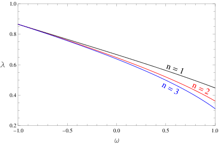
For the power law solution $a(t)\propto t^{q}$, the function $z$ defined in Eq. (44) becomes

With $z$ given by the above expression, the Mukhanov-Sasaki equation (37) can be expressed as

where

The general solution of the above equation can be expressed as

where $\mathrm{C}_{1}$ and $\mathrm{C}_{2}$ are constants of integration, $\mathrm{H}^{{}^{(1)}}_{\nu}\left(x\right)$ and $\mathrm{H}^{{}^{(2)}}_{\nu}\left(x\right)$ are Hankel functions of first and second kind, respectively. On imposing the Bunch-Davis initial condition that $u_{{}_{k}}=(2kc_{{}_{s}})^{-(1/2)}\exp\left[-ic_{{}_{s}}k\eta\right]$ at the sub-horizon scales $(\,-c_{{}_{s}}k\eta\,\gg\,1\,)$ leads to $\mathrm{C}_{2}=0$ and the above solution for the mode function $u_{{}_{k}}$ becomes

Similarly for the tensor perturbations, the solution of the Eq. (38), satisfying the Bunch-Davis initial condition turns out to be identical to $u_{{}_{k}}$, except for tensor perturbations $c_{{}_{s}}=1$. Therefore,

From the above solutions for mode functions $u_{{}_{k}}$ and $v_{{}_{k}}$, the scalar and tensor power spectrum defined in Eqs. (39) and (40), respectively, at the super horizon scales $(\,-c_{{}_{s}}k\eta\,\ll\,1\,)$ turns out to be

where

In the above equations $\Gamma(\nu)$ is Gamma function and $a_{{}_{1}}$ is a constant that appears in the equation describing the evolution of scalar factor in conformal time, viz. $a(\eta)=a_{{}_{1}}\left[-\eta\right]^{-q/(q-1)}$. The value of this parameter $a_{{}_{1}}$ in Eqs. (56) and (57) can be fixed using the CMB normalization, namely, $P_{{}_{S}}(k_{\ast})=2.2\times 10^{-9}$ at the pivot scale $k_{\ast}=0.05\,\mathrm{Mpc}^{-1}$ [4]. For $n=4$ and $q=60$, it turns out that $a_{{}_{1}}\simeq 4.4\times 10^{5}M_{p}^{-q/(q-1)}$. Since $a(\eta)=a_{{}_{1}}\left[-\eta\right]^{-q/(q-1)}$ implies that $a(t)=a_{\ast}(t/t_{\ast})^{q}$, it turns out that $a_{\ast}=a_{1}^{1-q}\left[t_{\ast}/(q-1)\right]^{q}$. Let $t_{\ast}=q/H_{\ast}$ be the time at which the pivot scale exit the cosmological horizon ($a_{\ast}H_{\ast}=k_{\ast}$), which in turn implies that

Therefore, the CMB normalized value of $a_{{}_{1}}$ can be used to determined the value of the Hubble parameter $H_{\ast}$ when the pivot scale exit the cosmological horizon. For $n=4$ and $q=60$, we find that $H_{\ast}=2.2\times 10^{-5}M_{p}$.

From Eqs. (54) and (55), the scalar and tensor spectral index, defined in Eqs. (41) and (42), respectively, turns out to be

This is exactly the same for the case of standard power law inflation driven by a canonical scalar field with an exponential potential [44, 45, 46] and one also gets the same $n_{{}_{S}}$ and $n_{{}_{T}}$ in the power law scenario in some non-canonical scalar field models such as those discussed in Refs. [14, 15, 32]. In fact, Eq. (58) is valid for any model of power law inflation based on the Lagrangian (2) but for which the parameters $c_{{}_{s}}^{2}$ and $\lambda$ defined in Eqs. (33) and (46), respectively, are identically constant. This simply follows from the fact that whenever $c_{{}_{s}}^{2}$ and $\lambda$ are constant, the solution (52) for the mode function $u_{{}_{k}}$ satisfy the Mukhanov Sasaki equation (37) during power law expansion and the resultant $n_{{}_{S}}$ (and $n_{{}_{T}}$) is the consequence of this solution for $u_{{}_{k}}$ (and $v_{{}_{k}}$).

Eqs. (54) and (55) lead to the following tensor-to-scalar ratio

It is evident from the above expression that unlike the spectral indices $n_{{}_{S}}$ and $n_{{}_{T}}$ which depends only on the value of $q$ in the power law solution $a(t)\propto t^{q}$, the tensor-to-scalar ratio $r$ also depends on the model parameters $c_{{}_{s}}^{2}$ and $\lambda$ defined in Eqs. (33) and (46), respectively. Therefore, $r$ contains the details of the dynamics of inflation and it can play an important role in distinguishing models of inflation [47].

Eqs. (58) and (59) imply the following consistency relation

where the expression for $c_{{}_{s}}^{2}$ and $\lambda$ for the Galilean power law inflation model (19) are given by Eqs. (48) and (49), respectively. Note that the above consistency relation is an exact result since no slow roll approximation is imposed.

In Fig. 2, the ratios $r/(8|n_{{}_{T}}|)$ and $r/(8c_{{}_{s}}|n_{{}_{T}}|)$ are plotted as a function of slow roll parameter $\varepsilon\equiv-\dot{H}/H^{2}$ for different models of power law inflation. In this figure, relation (60) is used for the Galilean power law model while for the power law scenario in k-inflation [15] and in the non-canonical scalar field model [32], the same relation (60) is used but with $\lambda=1$. This is justified from the analysis of Ref. [14]. For the power law inflation driven by a canonical scalar field $r=16/q$ [48] which leads to the following exact consistency relation $r=-8n_{{}_{T}}(q-1)/q$.

In the slow roll limit which corresponds to $q\gg 1$, the consistency relation (60) reduces to

In comparison, for the case of k-inflation, one gets $r\,=\,-8\,c_{{}_{s}}\,n_{{}_{T}}$. Therefore, as mentioned earlier, it is the $\lambda$ parameter defined in Eq. (46) which alters the consistency relation in G-inflation. Note that, although, the consistency relation (61) was derived for the power law inflation, it is approximately valid, in the slow roll limit, for a generic G-inflation model with Lagrangian (2). For the power law inflation driven by a Galilean field, the slow roll regime of the consistency relation (61) can be re-expressed as

References

- (1) A. A. Starobinsky, A new type of isotropic cosmological models without singularity, Phys. Lett. B 91 (1980) 99; A. H. Guth, Inflationary universe: A possible solution to the horizon and flatness problems, Phys. Rev. D 23 (1981) 347.
- (2) A. D. Linde, A new inflationary universe scenario: A possible solution of the horizon, flatness, homogeneity, isotropy and primordial monopole problems, Phys. Lett. B 108 (1982) 389; A. Albrecht and P. J. Steinhardt, Cosmology for Grand Unified Theories with Radiatively Induced Symmetry Breaking, Phys. Rev. Lett. 48 (1982) 1220; A. D. Linde, Phys. Lett. B, Chaotic inflation 129 (1983) 177.
- (3) V. F. Mukhanov and G. V. Chibisov, Quantum fluctuations and a nonsingular universe JETP Lett. 33 (1981) 532; S. W. Hawking, The development of irregularities in a single bubble inflationary universe, Phys. Lett. B 115 (1982) 295; A. A. Starobinsky, Phys. Lett. B Dynamics of phase transition in the new inflationary universe scenario and generation of perturbations, 117 (1982) 175; A. H. Guth and S.-Y. Pi, Fluctuations in the New Inflationary Universe, Phys. Rev. Lett. 49 (1982) 1110.
- (4) P. A. R. Ade, et. al., Planck 2013 results. XXII. Constraints on inflation, arXiv:1303.5082.
- (5) P. A. R. Ade, et. al., Planck 2013 results. XVI. Cosmological parameters, arXiv:1303.5076.
- (6) J. Martin, C. Ringeval and V. Vennin, Encyclopaedia Inflationaris, arXiv:1303.3787.
- (7) A. Mazumdar and J. Rocher, Particle physics models of inflation and curvaton scenarios, Phys. Rept. 497, 85 (2011) [arXiv: 1001.0993].
- (8) A. Riotto, Inflation and the theory of cosmological perturbations, arXiv: hep-ph/0210162
- (9) J. Martin, Inflationary cosmological perturbations of quantum-mechanical origin, Lect. Notes Phys. 669, 199 (2005) arXiv: hep-th/0406011
- (10) B. A. Bassett, S. Tsujikawa and D. Wands, Inflation dynamics and reheating, Rev. Mod. Phys. 78, 589 (2006) [arXiv: astro-ph/0507632].
- (11) W. H. Kinney, TASI Lectures on inflation, arXiv: 0902.1529.
- (12) L. Sriramkumar, An introduction to inflation and cosmological perturbation theory, Curr. Sci. 97 (2009) 868 [arXiv: 0904.4584].
- (13) D. Baumann, TASI Lectures on inflation, arXiv: 0907.5424.
- (14) J. Garriga and V. F. Mukhanov, Perturbations in k-inflation, Phys. Lett. B 458 (1999) 219 [hep-th/9904176].
- (15) C. Armendariz-Picon, T. Damour and V. Mukhanov, K-Inflation, Phys. Lett. B 458, 209 (1999) [arXiv:hep-th/9904075].
- (16) S. Unnikrishnan, V. Sahni and A. Toporensky, Refining inflation using non-canonical scalars, JCAP 1208 (2012) 018 [arXiv: 1205.0786].
- (17) S. Li and A. R. Liddle, Observational constraints on K-inflation models, JCAP 1210 (2012) 011 [arXiv: 1204.6214].
- (18) C. Deffayet, O. Pujolas, I. Sawicki and A. Vikman, Imperfect Dark Energy from Kinetic Gravity Braiding, JCAP 1010, 026 (2010) [arXiv: 1008.0048].
- (19) T. Kobayashi, M. Yamaguchi and J. Yokoyama, Inflation Driven by the Galileon Field, Phys. Rev. Lett. 105, 231302 (2010) [arXiv: 1008.0603].
- (20) C. Deffayet, S. Deser, G. Esposito-Farese, Generalized Galileons: All scalar models whose curved background extensions maintain second-order field equations and stress tensors, Phys. Rev. D 80, 064015 (2009) [arXiv: 0906.1967].
- (21) D. Lovelock, The Einstein tensor and its generalizations, J. Math. Phys. 12, 498 (1971).
- (22) A. Nicolis, R. Rattazzi and E. Trincherini, Galileon as a local modification of gravity, Phys. Rev. D 79, 064036 (2009) [arXiv: 0811.2197].
- (23) C. Deffayet, G. Esposito-Farese and A. Vikman, Covariant Galileon, Phys. Rev. D 79, 084003 (2009) [arXiv: 0901.1314].
- (24) A. De-Felice and S. Tsujikawa, theories, Living Rev. Rel. 13, 3 (2010) [arXiv: 1002.4928].
- (25) A. A. Starobinsky, Spectrum of relict gravitational radiation and the early state of the universe, JETP Lett. 30 (1979) 682.
- (26) A. A. Starobinsky, Cosmic Background Anisotropy Induced by Isotropic Flat-Spectrum Gravitational-Wave Perturbations, Soviet Astronomy Lett. 11 (1985) 133.
- (27) M. Sasaki and E. D. Stewart, A General Analytic Formula for the Spectral Index of the Density Perturbations Produced during Inflation Prog. Theor. Phys. 95, 71 (1996) [astro-ph/9507001].
- (28) V. Mukhanov and A. Vikman, Enhancing the tensor-to-scalar ratio in simple inflation, JCAP 0602, 004 (2006) [astro-ph/0512066].
- (29) E. Babichev, V. Mukhanov and A. Vikman, k-Essence, superluminal propagation, causality and emergent geometry, JHEP 0802, 101 (2008) [arXiv: 0708.0561]; G. Ellis, R. Maartens and M. MacCallum, Causality and the speed of sound, Gen. Rel. Grav. 39, 1651 (2007) [arXiv:gr-qc/0703121]; C. Bonvin, C. Caprini and R. Durrer, No-go theorem for k-essence dark energy, Phys. Rev. Lett. 97, 081303 (2006) [astro-ph/0606584]; J. U. Kang, V. Vanchurin and S. Winitzki, Attractor scenarios and superluminal signals in k-essence cosmology, Phys. Rev. D 76, 083511 (2007) [arXiv:0706.3994].
- (30) K. Kamada, T. Kobayashi, M. Yamaguchi and J. Yokoyama, Higgs G-inflation, Phys. Rev. D 83, 083515 (2011) [arXiv:1012.4238].
- (31) T. Kobayashi and T. Takahashi, Large Tensor-to-Scalar Ratio in Small-Field Inflation, Phys. Rev. Lett. 110, 231101 (2013) [arXiv: 1303.0242].
- (32) S. Unnikrishnan and V. Sahni, Resurrecting power law inflation in the light of Planck results, JCAP in press, [arXiv: 1305.5260].
- (33) J. D. Barrow, Graduated inflationary universes, Phys. Lett. B235 (1990) 40.
- (34) A. Muslimov, On the scalar field dynamics in a spatially flat Friedman universe, Class. Quant. Grav. 7 (1990) 231.
- (35) J. .M. Bardeen, Gauge-invariant cosmological perturbations, Phys. Rev. D 22, 1882 (1980).
- (36) H. Kodama and M. Sasaki, Cosmological Perturbation Theory, Prog. Theor. Phys. Suppl. 78, 1 (1984).
- (37) V. F. Mukhanov, H. A. Feldman and R. H. Brandenberger, Theory of cosmological perturbations, Phys. Rep. 215, 203 (1992).
- (38) Yi-Fu Cai, D. A. Easson and R. Brandenberger, Towards a Nonsingular Bouncing Cosmology, JCAP 08, 020 (2012) [arXiv: 1206.2382].
- (39) A. Naruko and M. Sasaki, Conservation of the nonlinear curvature perturbation in generic single-field inflation, Class. Quant. Grav. 28, 072001 (2011) [arXiv: 1101.3180].
- (40) M. Alishahiha, E. Silverstein and D. Tong, DBI in the Sky, Phys. Rev. D 70 (2004) 123505 [hep-th/0404084].
- (41) D. A. Steer and F. Vernizzi, Tachyon inflation: tests and comparison with single scalar field inflation, Phys. Rev. D 70, 043527 (2004) [arXiv: hep-th/0310139].
- (42) E. D. Stewart, Spectrum of density perturbations produced during inflation to leading order in a general slow-roll approximation, Phys. Rev. D 65, 103508 (2002) [arXiv: astro-ph/0110322].
- (43) W. Hu, Generalized Slow Roll for Non-Canonical Kinetic Terms, Phys. Rev. D 84 (2011) 027303 [arXiv:1104.4500].
- (44) L. F. Abbott and M. B. Wise, Constraints on generalized inflationary cosmologies, Nucl. Phys. B 244 (1984) 541.
- (45) F. Lucchin and S. Matarrese, Power-law inflation, Phys. Rev. D 32 (1985) 1316.
- (46) V. Sahni, Scalar field fluctuations and infrared divergent states in cosmological models with power law expansion, Class. Quant. Grav. 5 (1988) L113; Energy density of relic gravity waves from inflation, Phys. Rev. D 42 (1990) 453.
- (47) S. Hotchkiss, A. Mazumdar and S. Nadathur, Observable gravitational waves from inflation with small field excursions, JCAP 02, 008 (2012) [arxiv: 1110.5389]; S. Choudhury and A. Mazumdar, An accurate bound on tensor-to-scalar ratio and the scale of inflation, arXiv: 1306.4496; S. Choudhury, A. Mazumdar and S. Pal, Low & High scale MSSM inflation, gravitational waves and constraints from Planck JCAP 07, 041 (2013) [arxiv: 1305.6398].
- (48) T. Souradeep and V. Sahni, Density Perturbations, Gravity Waves and the Cosmic Microwave Background, Mod. Phys. Lett. A7 (1992) 3541 [hep-ph/9208217].
- (49) K. Kamada, T. Kobayashi, T. Kunimitsu, M. Yamaguchi and J. Yokoyama, Graceful exit from Higgs G-inflation, [arXiv: 1309.7410].
- (50) O. Pujolas, I. Sawicki and A Vikman, The Imperfect Fluid behind Kinetic Gravity Braiding, JHEP 1111 (2011) 156 [arXiv: 1103.5360].
- (51) D. A. Easson, I. Sawicki and A. Vikman, When Matter Matters, JCAP 07, 014 (2013) [arXiv: 1304.3903]
- (52) P. A. R. Ade, et. al., Planck 2013 Results. XXIV. Constraints on primordial non-Gaussianity, arXiv:1303.5084.
- (53) T. Kobayashi, M. Yamaguchi and J Yokoyama, Generalized G-inflation: Inflation with the most general second-order field equations, Prog. Theor. Phys. 126, 511 (2011) [arxiv: 1105.5723].
- (54) X. Chen, M. Huang, S. Kachru and G. Shiu, Observational Signatures and Non-Gaussianities of General Single Field Inflation, JCAP 0701 (2007) 002 [hep-th/0605045].
- (55) T. Kobayashi, M. Yamaguchi and J Yokoyama, Primordial non-Gaussianity from G-inflation, Phys. Rev. D 83, 103524 (2011) [arxiv: 1103.1740].
- (56) X. Gao, T. Kobayashi, M. Shiraishi, M. Yamaguchi, J. Yokoyama and S. Yokoyama, Full bispectra from primordial scalar and tensor perturbations in the most general single-field inflation model, Prog. Theor. Exp. Phys. 053E03 (2012) [arxiv: 1207.0588].
- (57) K. Kamada, T. Kobayashi, T. Takahashi, M. Yamaguchi and J. Yokoyama, Generalized Higgs inflation, Phys. Rev. D 86, 023504 (2012) [arxiv: 1203.4059].
- (58) W. Hu, Structure Formation with Generalized Dark Matter, Astrophys. J 506, 485 (1998) [arXiv: astro-ph/9801234].