Numerical methods for parameter identification in stationary radiative transferThanks: †Numerical Analysis and Scientific Computing, Department of Mathematics, TU Darmstadt, Dolivostr. 15, 64293 Darmstadt.
Email: egger,schlottbom@mathematik.tu-darmstadt.de
Abstract.
We consider the identification of scattering and absorption rates in the stationary radiative transfer equation. For a stable solution of this parameter identification problem, we consider Tikhonov regularization within Banach spaces. A regularized solution is then defined via an optimal control problem constrained by an integro partial differential equation. By establishing the weak-continuity of the parameter-to-solution map, we are able to ensure the existence of minimizers and thus the well-posedness of the regularization method. In addition, we prove certain differentiability properties, which allow us to construct numerical algorithms for finding the minimizers and to analyze their convergence. Numerical results are presented to support the theoretical findings and illustrate the necessity of the assumptions made in the analysis.
Keywords: parameter estimation, radiative transfer, Tikhonov regularization
AMS Subject Classification: 65M32, 35Q93, 49N45
1. Introduction
We consider the stationary radiative transfer equation
| (1) |
which models the equilibrium distribution of an ensemble of mutually non-interacting particles in an isotropically scattering medium. The function here denotes the density of particles at a point moving in direction , and the symbol denotes derivatives with respect to the spatial variables only. The medium is characterized by rates and of absorption and scattering. Interior sources are represented by and the inflow of particles over the boundary is modeled by
| (2) |
where is the unit outward normal at a point . Problems of the form (1)–(2) arise in various applications, e.g., in neutron physics [6], in medical imaging [2], in astrophysics [7, 8, 29], or climatology [26].
In this paper, we are interested in the determination of the material properties, encoded in the spatially varying parameters and from measurements
| (3) |
of the outflow of particles over the boundary. This parameter identification problem can be formally written as an abstract operator equation
| (4) |
where is a given measurement, and denotes the parameter-to-solution map defined by solving (1)–(2). Note that and also depend on the sources and .
Due to the many important applications, the inverse problem (4) has been investigated intensively in the literature. To give an impression of the basic properties of the problem, let us summarize some of the most important results: The parameters , can be uniquely identified, if sufficiently many measurements are available [9]. In particular, multiple excitations and are required. The stability of the identification process with respect to perturbations in the data has been investigated in [4, 5, 28]. In general, the stability will be very low. Various methods to numerically solve the parameter identification problem have been proposed as well [12, 25, 36].
It is by now well understood that solving (4) is an ill-posed problem. For a stable solution, we will therefore consider Tikhonov regularization, to be precise, we define approximate solutions via minimization problems of the form
| (5) |
where and denote some a-priori information about the unknown parameters , . The domain will be defined below. This can be seen as an optimal control problem governed by an integro partial differential equation.
The main focus of this manuscript is to establish the existence of minimizers for (5) and thus to ensure the well-posedness of the regularized problem. We will also show that (5) is a regularization method in the sense of [16]. In addition, we will investigate iterative algorithms to approximate the minimizers. The key ingredient for our arguments is a careful analysis of the mapping properties of the parameter-to-solution map . We will establish its strong and weak continuity with respect to the corresponding and topologies, and derive various differentiability results. Let us mention that for particular choices of the parameter and measurement spaces, the stable solution of the inverse problem (4) by Tikhonov regularization has been considered already in [11, 33, 35]. Our results here are more general and require a much finer analysis of the operator . We will make more detailed comments on this in the following sections. As a numerical method for minimizing the Tikhonov functional, we consider a variation of the iteratively regularized Gauß-Newton method. This method has been investigated in the framework of regularization methods in [3, 23]. Here, we investigate its properties for minimization of the regularized functional.
The outline of the manuscript is as follows: in Section 2, we introduce the necessary notation and recall some existence results for the transport equation. After fixing the domain of , we proof our main results about continuity, weak continuity, and differentiability of in Section 3. We turn back to the optimal control problem in Section 4 and investigate iterative methods for its solution in Section 5. For illustration of our theoretical considerations, some numerical results are presented in Section 6, and we conclude with a short summary.
2. Preliminaries
Let us introduce the basic notions and the functional analytic setting in which we investigate the solvability of the radiative transfer problem. The following physically reasonable and quite general assumptions will be used throughout the paper.
- (A1)
is a bounded domain with Lipschitz boundary.
- (A2)
and for a.e. with some constant .
- (A3)
and for a.e. with some constant .
Since is Lipschitz continuous, we can define for almost every the outward unit normal vector . We denote by the boundary of the tensor product domain and decompose into an in- and outflow part by
| (6) |
We will search for solutions of the radiative transfer problem (1)–(2) in the space
which is equipped with the graph norm
Here denotes a weighted -space with weighting function . Note that for , the spaces are complete and that is a Hilbert space. Due to the boundedness of the spatial domain , the embedding is continuous for , but neither nor are compact. For functions and with , we obtain the integration-by-parts formula
| (7) |
As usual, the symbol is used for the integral of the product of two functions over some domain . Applying this formula to and yields
| (8) |
i.e., the outflow trace of functions in is well-defined and the trace operator is continuous from to . Via Hölder’s inequality, we immediately obtain
Lemma 2.1.
The operator defined in (3) is linear and bounded.
Let us introduce the transport operator
which models the flow of particles in direction , and the averaging operator
describing the scattering of particles by the background medium. The collision operator
then models the total interaction of particles with the medium. Note, that depends linearly on the parameters and , and we will sometimes write to emphasize this dependence. For later reference, let us summarize some basic properties of the operators, which follow more or less directly from their definition; see [10, 14] for details.
Lemma 2.2.
Let (A1)–(A3) hold. Then the operators , , and are bounded linear operators. Moreover, and are self-adjoint and is positive on .
As already mentioned, the energy spaces are not compactly embedded in . The following result, known as averaging lemma, serves as a substitute and will play a key-role in our analysis.
Lemma 2.3.
For any the averaging operator is compact. Here denotes the subspace of with vanishing inflow boundary conditions.
We refer to [18] for a proof of this result. Let us mention that averaging lemmas also play a key role for the spectral analysis of the radiative transfer equation.
Using the operators defined above, the radiative transfer problem (1)–(2) can be written in compact form: Given and , find such that
| (9) | ||||||
| (10) |
The two equations have to hold in the sense of and , respectively. The existence and uniqueness of solutions for this problem is established next.
Theorem 2.4.
3. Properties of the parameter-to-solution map
In this section, we investigate the mapping properties of the parameter-to-solution map
| (11) |
where is the solution of (9)–(10) for given data and . The domain of is defined by
Note that the operator also depends on the choice of and on the data and . For ease of presentation, we will emphasize this dependence only if necessary.
3.1. Continuity
Let us start with presenting some results about the continuity of with respect to the strong and weak topologies. The latter case will play a fundamental role in the analysis of the optimal control problem later on.
Theorem 3.1 (Continuity).
Let and assume that and . Then is continuous as mapping from to .
Proof.
Let and such that . Furthermore, denote by and the solutions of (9)–(10) with parameters and , respectively. Then
Since in , we can choose a subsequence, again denoted by , such that a.e. in and consequently a.e. in . Since is uniformly bounded, Lebesgue’s dominated convergence theorem ensures in . Similarly, in . The uniform a-priori estimate of Theorem 2.4 then yields in . ∎
We will show next, that the parameter-to-solution map is also continuous in the weak topology. This directly implies the weak-lower semi-continuity of the Tikhonov functional and thus yields the well-posedness of the regularization method. The proof of the result heavily relies on the compactness provided by the averaging lemma.
Theorem 3.2 (Weak continuity).
Let and assume that and . Then is weakly continuous, i.e., if in , then and in .
Proof.
Since is closed and convex, is weakly closed and . Now let denote the unique solutions of (9)–(10) with parameters , and , , respectively. Then the difference satisfies the transport problem
| (12) |
with right-hand side defined by
By Theorem 2.4, the operator is continuously invertible. It thus remains to prove that . Multiplying the first term with and integrating yields
Now by Lemma 2.3, we obtain strongly in . From this we conclude that and as a consequence . The term involving can be treated in a similar way. ∎
For the following quantitative estimate, we require some slightly stronger assumptions on the source terms. This kind of regularity seems to be necessary since due to its hyperbolic type the transport equation does not possess a regularizing effect.
Theorem 3.3.
Let and . Then for any the operator is Lipschitz continuous as a mapping from to .
3.2. Differentiability
As a next step, we investigate differentiability of the parameter-to-solution map. We call a parameter pair an admissible variation for , if the perturbed parameters for .
Theorem 3.4.
Proof.
Let denote the solution of (9)–(10) for parameters and sufficiently small and let . Then
and on . By Theorem 2.4 we thus obtain
The continuity of the parameter-to-solution map, and the integrability condition on the data, yields in from which we conclude that in as . The estimate (14) follows again from Theorem 2.4. ∎
One can see from (13) that depends linearly on the variation . By the continuous extension principle, the operator can then be extended to a bounded linear operator , which we call the derivative of in the following.
Theorem 3.5.
Let and and assume that and . Then is Lipschitz continuous, i.e., for , there holds
Proof.
Let , , and let , , be the solutions of the sensitivity problems in Theorem 3.4 for some admissible direction . Then satisfies (13) with . Using Hölder’s inequality the two parts of can be estimated individually by
| (15) | ||||
| (16) |
Using Theorem 3.3 and Theorem 3.4 we then obtain via the triangle inequality
The Lipschitz estimate now follows from the a-priori estimates stated in Theorem 2.4. ∎
Differentiability of has already been proven in [11], but under more restrictive assumptions and only for , which turns out to be the simplest case. The proofs of [11] cannot be applied to the more general setting considered here. By carefully inspecting the estimates (15)–(16), using assumptions (A2)–(A3), Hölder’s inequality, and interpolation, we obtain
Corollary 3.6.
Let and and assume that and . Then is Hölder continuous with Hölder exponent .
This estimate will allow us to obtain convergence of iterative minimization algorithms under very general conditions. With the same techniques as used to prove Theorem 3.5, one can also analyze higher order derivatives. For later reference let us state a result about the existence of the Hessian.
Theorem 3.7.
Let for some and assume that and . Then is twice continuously differentiable and is given by
where is the unique solution of
Moreover, is Lipschitz continuous w.r.t. its arguments and
with depending only on the domain, the bounds for the parameters, and the data.
Like above, the Hessian should first be defined for admissible parameter variations and then be extended to a bounded bilinear map. The estimate then follows in the same way as the Lipschitz estimate for the first derivative. We will utilize the properties of the Hessian to show local convexity of the regularized functional (5) in a Hilbert space setting.
4. The optimal control problem
Let us recall the definition of the optimal control problem
defined by minimizing the Tikhonov functional for some . Based on the results about the mapping properties of the parameter to solution map and the observation operator , we will now comment on the existence and stability of minimizers. The arguments are rather standard, and we only sketch the main points. Let us refer to [16, 17] for details and proofs.
4.1. Existence of Minimizers
By weak continuity of and weak lower semi-continuity of norms, the Tikhonov functional is weakly lower semi-continuous and bounded from below. Due to the box constraints and the reflexivity of , , the domain is weakly compact. This yields the existence of a minimizer for any .
4.2. Stability of Minimizers
The minimizers are stable w.r.t. perturbations in the following sense: For and there exists a sequence of minimizers converging weakly to a minimizer . This follows from the weak compactness of and weak continuity of . If , then we can obtain strong convergence.
4.3. Convergence of Minimizers
4.4. Remarks and generalizations
Note that, in general, uniqueness of solutions for the inverse problem (4) or of minimizers for the optimal control problem (5) cannot be expected. We will discuss this issue in more detail in the next section. Also note that, with the same arguments as above, we can analyze minimization problems of the form
where is some more general regularization functional. One particular choice will be considered in more detail in the next section. Total variation regularization is frequently used in image reconstruction; for an analysis see for instance [1]. Due to the continuous embedding of and in certain spaces, the statements about existence, stability, and convergence of minimizers made above also hold true for these choices. Our results thus generalize those of [35]. Note however, that in dimension , we cannot obtain Lipschitz- or Hölder continuity of the derivative for -regularization, while for we even obtain Lipschitz continuous second derivatives. This is our guideline for the setting of the next section.
5. Iterative minimization algorithms
To ensure convergence of minimization algorithms, one has to impose some more restrictive conditions. In order to motivate the crucial assumptions, let us recall a basic convergence rate result from nonlinear regularization theory [16, 17]. To simplify the presentation, we restrict ourselves to a Hilbert space setting and consider the Tikhonov functional
| (17) |
Note that due to the continuous embedding of into in dimension , we can use all properties of derived in Section 3 for and . In particular, we infer from Theorem 3.5 and Theorem 3.7 that has Lipschitz-continuous first and second derivatives.
5.1. Convergence Rates for Minimizers
It is well-known that quantitative estimates for convergence can only be obtained under some kind of source condition. We therefore assume in the following that there exists some such that
| (18) |
where solves (4) and is the Lipschitz constant of ; see Theorem 3.5. From the abstract theory of nonlinear Tikhonov regularization [16, 17], we deduce that
where are corresponding minimizers of the Tikhonov functional with . Note that the best possible rate one could expect for the error in the parameters is , and for the residual is , if (18) is not fulfilled.
5.2. An iterative algorithm for computing a minimizer
For minimizing the Tikhonov functional (17), we consider a projected Gauß-Newton (PGN) method. To ease the notation, we use and . The method then reads
Here denotes the metric projection onto with respect to the -norm and is the Hilbert space adjoint of the linearized parameter-to-measurement operator. As usual, can be computed via the solution of an adjoint problem similar to (13). A detailed analysis of the PGN iteration in the framework of iterative regularization methods can be found [3, 22]. Here, we consider this algorithm for the approximation of minimizers of the Tikhonov functional (17). To promote global convergence, we choose a geometrically decaying sequence of regularization parameters. If the source condition (18) holds with sufficiently small, then
with a constant not depending on or . For , we recover the usual convergence rate statement of the iterative regularization method without data noise [3, Chapter 4]. For , the iteration is bounded but convergence is not so clear.
5.3. Local convexity and convergence to minimizers
We will now explain that for and under the source condition (18), the PGN iteration converges to a local minimizer of the Tikhonov functional. Consider the Hessian of the Tikhonov functional given by
One can easily see that, if is two-times differentiable and the norm of the residual is sufficiently small, such that , then the Hessian is positive definite. Now, by the Lipschitz estimate for the first derivative we deduce that , and from the convergence rate estimates for nonlinear Tikhonov regularization we have . Hence we conclude that, if the source condition (18) is valid and is sufficiently small, then the Tikhonov functional is locally convex in a neighborhood of the minimizers . From the estimates for and and by the Lipschitz estimate for the first derivative, one can actually conclude that the region of convexity is always reached after a finite number of iterations. For a detailed analysis using similar arguments see [30]. In the area of convexity, the linear convergence follows with standard arguments.
5.4. Remarks and Extensions
Using the abstract theory of regularization methods in Banach spaces [20], the statements of the section can in principle be extended to the - setting considered earlier; see also [31, 32, 34]. The required convergence rates results for the GN method in Banach spaces have been established in [21, 24]. At the end of our discussion, let us mention that also projected gradient methods in combination with appropriate rules for the choice for the stepsize can be used for minimizing the Tikhonov functional. For these methods, convergence to stationary points can be established even without a source condition and merely under Hölder continuity of the derivative [19]. The same holds true for the PGN method [13].
6. Computational Experiments
To illustrate the theoretical results of the previous sections, we will present some numerical experiments in the following.
6.1. Discretization
For discretization of the radiative transfer problem (1)–(2) we employ the -FEM method. This is a Galerkin approximation using a truncated spherical harmonics expansion with respect to the direction and a mixed finite element approximation for the corresponding spatially dependent Fourier coefficients. Due to the variational character of the method, one can systematically obtain consistent discretizations of the operator parameter-to-solution operator , its derivative , and the adjoint . Let us refer to [14, 27, 36] for an analysis of the method and details on the implementation.
6.2. Test example and choice of parameters
We consider the setup depicted in Figure 1: The computational domain is a two-dimensional circle with radius mm. The absorption parameter is in the range of mm-1 to mm-1. The scattering ranges from mm-1 to mm-1. This order of magnitude is typical for applications in optical tomography [2]. The data are generated by sequentially illuminating the object by one of the sources and recording the outgoing light on the th detector for prescribed parameters and , i.e.
| (19) |
Here is the photon density generated by the th source and models the area of the th detector; see Figure 1 for the arrangements of sources and detectors. For our numerical experiments, we choose a sequence of regularization parameters with and . As initial guess, we use the constant functions mm-1 and mm-1.


6.3. Generation of Data and Non-uniqueness
Note that our choice of parameters and depicted in Figure 1 cannot be expected to satisfy the source condition (18). To be able to observe convergence rates, we therefore compute in a first step a minimizer of the Tikhonov functional with . The result of this preprocessing step is depicted in Figure 2.


Let us mention that we obtain different reconstructions when changing the initial value , which is a clear indication of non-uniqueness in for the inverse problem (4); see also [2] for a theoretical explanation. Using the calibrated parameter as truth-approximation, we then compute the measurements as in (19). The relative error in the data corresponding to the parameters depicted in Figure 1 and 2 is less then %. This indicates the ill-posedness and possible non-uniqueness for the inverse problem.
6.4. Convergence rates for minimizers
In a first numerical test, we want to demonstrate the convergence of the minimizers of the Tikhonov functional (17) towards the correct parameter pair generated in the preprocessing step. We denote by
the observed residuals and errors in the regularized solutions. The convergence rates for the residual and the error can be seen in Figure 3.


As predicted by theory, we observe the asymptotic rate for the error . The convergence rate for the residuals is slightly less than the expected rate .
6.5. Convergence of PGN method for fixed
With the second experiment, we would like to demonstrate the linear convergence of the PGN method to the minimizer of the Tikhonov functional. To do so, we compute for the minimizers by iterating the PGN method until convergence. We then restart the iteration to create a sequence of PGN iterates defined as in Section 5.2 with . The residuals and the errors in the th iteration given by
are depicted in Figure 4. For comparison, we also display the theoretical convergence curve.

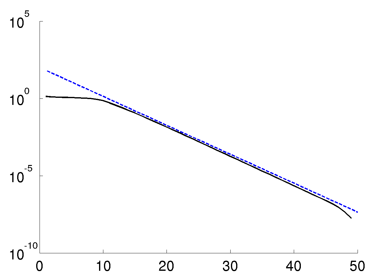
In the first iterations, is still rather large and the iterates stay within the vicinity of the initial guess. After decreased sufficiently, the convergence of the error gets linear, i.e. for some . The residuals do not converge to zero here, since the minimizer does not solve the inverse problem (4) exactly. The residuals and the errors are however monotonically decreasing, which highlights the stability of the method.
7. Conclusions
In this paper we investigated numerical methods for reconstructing scattering and absorption rates in stationary radiative transfer from boundary observations. For a stable solution of this inverse problem, we considered Tikhonov regularization which leads to an optimal control problem constrained by an integro partial differential equation. Using some sort of compactness provided by the averaging lemma, we were able to prove the weak continuity of the parameter-to-solution mapping. This allows us to show existence and stability of minimizers. We also established important differentiability properties which are required for the convergence of iterative minimization algorithms. We discussed the convergence of a projected Gauß-Newton method. Under the typical source condition, which is also required for nonlinear regularization theory, we could establish local convexity of the Tikhonov functional in the vicinity of minimizers, and thus obtained local linear convergence of the projected Gauß-Newton method. It would be interesting to know, if convergence of iterative minimization algorithms can be shown without some sort of source condition.
References
- [1] Acar, R., Vogel, C.R.: Analysis of bounded variation penalty methods for ill-posed problems. Inverse Problems 10, 1217–1229 (1994)
- [2] Arridge, S.R.: Optical tomography in medical imaging. Inverse Problems 15(2), R41–R93 (1999)
- [3] Bakushinsky, A.B., Kokurin, M.Y.: Iterative Methods for Approximate Solution of Inverse Problems, Mathematics and its Applications, vol. 577. Springer, Dordrecht (2004)
- [4] Bal, G.: Inverse transport from angularly averaged measurements and time harmonic isotropic sources. In: A.L. Y. Censor M. Jiang (ed.) Mathematical Methods in Biomedical Imaging and Intesity-Modulated Radiation Therapy, CRM, pp. 19–35. Scuola Normale Superiore Pisa, Italy (2008)
- [5] Bal, G., Jollivet, A.: Stability estimates in stationary inverse transport. Inverse Probl. Imaging 2(4), 427–454 (2008)
- [6] Case, K.M., Zweifel, P.F.: Linear transport theory. Addison-Wesley Publishing Co., Reading (1967)
- [7] Cercignani, C.: The Boltzmann Equation and Its Applications. Springer-Verlag, Berlin (1988)
- [8] Chandrasekhar, S.: Radiative Transfer. Dover Publications, Inc. (1960)
- [9] Choulli, M., Stefanov, P.: An inverse boundary value problem for the stationary transport equation. Osaka J. Math. 36(1), 87–104 (1998)
- [10] Dautray, R., Lions, J.L.: Mathematical Analysis and Numerical Methods for Science and Technology, Evolution Problems II, vol. 6. Springer, Berlin (1993)
- [11] Dierkes, T., Dorn, O., Natterer, F., Palamodov, V., Sielschott, H.: Fréchet derivatives for some bilinear inverse problems. SIAM J. Appl. Math. 62(6), 2092–2113 (2002)
- [12] Dorn, O.: A transport-backtransport method for optical tomography. Inverse Problems 14, 1107–1130 (1998)
- [13] Egger, H., Schlottbom, M.: Efficient reliable image reconstruction schemes for diffuse optical tomography. Inv. Probl. Sci. Engrg. 19, 155–180 (2011)
- [14] Egger, H., Schlottbom, M.: A mixed variational framework for the radiative transfer equation. Mathematical Models and Methods in Applied Sciences 03(22), 1150,014 (2012). DOI 10.1142/S021820251150014X. URL http://dx.doi.org/10.1142/S021820251150014X
- [15] Egger, H., Schlottbom, M.: An theory for stationary radiative transfer. Applicable Analysis (2013). DOI 10.1080/00036811.2013.826798
- [16] Engl, H.W., Hanke, M., Neubauer, A.: Regularization of inverse problems, Mathematics and its Applications, vol. 375. Kluwer Academic Publishers Group, Dordrecht (1996)
- [17] Engl, H.W., Kunisch, K., Neubauer, A.: Convergence rates for Tikhonov regularization of nonlinear ill-posed problems. Inverse Problems 5, 523–540 (1989)
- [18] Golse, F., Lions, P.L., Perthame, B., Sentis, R.: Regularity of the moments of the solution of a transport equation. Journal of Functional Analysis 76(1), 110–125 (1988). DOI 10.1016/0022-1236(88)90051-1
- [19] Hinze, M., Pinnau, R., Ulbrich, M., Ulbrich, S.: Optimization with PDE Constraints, Mathematical Modelling: Theory and Applications, vol. 23. Springer Science + Business Media B.V. (2009)
- [20] Hofmann, B., Kaltenbacher, B., Pöschl, C., Scherzer, O.: A convergence rates result for tikhonov regularization in banach spaces with non-smooth operators. Inv. Prob. 23, 987–1010 (2007)
- [21] Kaltenbacher, B., Hofmann, B.: Convergence rates for the iteratively regularized gauss–newton method in banach spaces. Inverse Problems 26(3), 035,007 (2010). URL http://stacks.iop.org/0266-5611/26/i=3/a=035007
- [22] Kaltenbacher, B., Neubauer, A.: Convergence of projected iterative regularization methods for nonlinear problems with smooth solutions. Inverse Problems 22, 1105–1119 (2006)
- [23] Kaltenbacher, B., Neubauer, A., Scherzer, O.: Iterative Regularized Methods for Nonlinear Ill-Posed Problems, Radon Series on Computational and Applied Mathematics, vol. 6. Walter de Gruyter (2008)
- [24] Kaltenbacher, B., Schöpfer, F., Schuster, T.: Iterative methods for nonlinear ill-posed problems in Banach spaces: convergence and applications to parameter identification problems. Inverse Problems 25, 065,003 (19pp) (2009)
- [25] Klose, A.D., Hielscher, A.H.: Iterative reconstruction scheme for optical tomography based on the equation of radiative transfer. Med. Phys. 26(8), 1698–1707 (1999)
- [26] Kondratyev, K.Y.: Radiation in the Atmosphere. Academic Press (1969)
- [27] Lewis, E.E., Miller Jr., W.F.: Computational Methods of Neutron Transport. John Wiley & Sons, Inc., New York Chichester Brisbane Toronto Singapore (1984)
- [28] McDowall, S., Stefanov, P., Tamasan, A.: Stability of the gauge equivalent classes in inverse stationary transport. Inverse Problems 26(2), 025,006 (2010). URL http://stacks.iop.org/0266-5611/26/i=2/a=025006
- [29] Peraiah, A.: An Introduction to Radiative Transfer – Methods and applications in astrophysics. Cambridge University Press (2004)
- [30] Ramlau, R.: TIGRA – an iterative algorithm for regularizing nonlinear ill-posed problems. Inverse Problems 19, 433–465 (2003)
- [31] Resmerita, E.: Regularization of ill-posed problems in banach spaces: convergence rates. Inverse Problems 21(4), 1303 (2005). URL http://stacks.iop.org/0266-5611/21/i=4/a=007
- [32] Scherzer, O., Grasmair, M., Grossauer, H., Haltmeier, M., Lenzen, F.: Variational Methods in Imaging. Springer (2009)
- [33] Schlottbom, M.: On forward and inverse models in optical tomography. Ph.D. thesis, RWTH Aachen (2011). URL http://darwin.bth.rwth-aachen.de/opus3/volltexte/2011/3857/
- [34] Schuster, T., Kaltenbacher, B., Hofmann, B., Kazimierski, K.S.: Regularization Methods in Banach Spaces. De Gruyter (2012)
- [35] Tang, J., Han, W., Han, B.: A theoretical study for RTE-based parameter identification problems. Inverse Problems 29(9), 095,002 (2013). URL http://stacks.iop.org/0266-5611/29/i=9/a=095002
- [36] Wright, S., Schweiger, M., Arridge, S.R.: Reconstruction in optical tomography using approximations. Meas. Sci. Technol. 18, 79–86 (2007)