The moments of the single inclusive momentum distribution of hadrons in QCD jets, are studied in the next-to-modified-leading-log approximation (NMLLA) including next-to-leading-order (NLO) corrections to the $\alpha_{\rm s}$ strong coupling. The evolution equations are solved using a distorted Gaussian parametrisation, which successfully reproduces the spectrum of charged hadrons of jets measured in $e^{+}e^{-}$ collisions. The energy dependencies of the maximum peak, multiplicity, width, kurtosis and skewness of the jet hadron distribution are computed analytically. Comparisons of all the existing jet data measured in $e^{+}e^{-}$ collisions in the range $\sqrt{\rm s}\approx$ 2–200 GeV to the NMLLA $+$ NLO^∗ predictions allow one to extract a value of the QCD parameter $\Lambda_{{}_{\rm QCD}}$ , and associated two-loop coupling constant at the Z resonance $\alpha_{\rm s}(\rm m^{2}_{{}_{\rm Z}})$ = 0.1195 $\pm$ 0.0022, in excellent numerical agreement with the current world average obtained using other methods.

1 Introduction

One of the most ubiquitous manifestations of the fundamental degrees of freedom of Quantum Chromodynamics (QCD), quark and gluons, are the collimated bunches of hadrons (“jets”) produced in high-energy particle collisions. The evolution of a parton into a final distribution of hadrons is driven by perturbative dynamics dominated by soft and collinear gluon bremsstrahlung [1, 2] followed by the final conversion of the radiated partons into hadrons at non-perturbative scales approaching $\Lambda_{{}_{\rm QCD}}\approx$ 0.2 GeV. The quantitative description of the distribution of hadrons of type $h$ in a jet is encoded in a (dimensionless) fragmentation function (FF) which can be experimentally obtained, e.g. in $e^{+}e^{-}$ collisions at c.m. energy $\sqrt{\rm s}$ , via

D^{\rm h}(\ln(1/x),\rm s)=\frac{d\sigma(ee\to hX)}{\sigma_{\rm tot}\,d\ln(1/x)},

where $x=2\,p_{h}/\sqrt{\rm s}$ is the scaled momentum of hadron $h$ , and $\sigma_{\rm tot}$ the total $e^{+}e^{-}$ hadronic cross section. Its integral over $x$ gives the average hadron multiplicity in jets. Writing the FF as a function of the (log of the) inverse of $x$ , $\xi=\ln(1/x)$ , emphasises the region of relatively low momenta that dominates the spectrum of hadrons inside a jet. Indeed, the emission of successive gluons inside a jet follows a parton cascade where the emission angles decrease as the jet evolves towards the hadronisation stage, the so-called “angular ordering” [3, 1, 4]. Thus, due to QCD colour coherence and interference of gluon radiation, not the softest partons but those with intermediate energies ( $E_{h}\propto E_{\rm jet}^{0.3}$ ) multiply most effectively in QCD cascades [4]. As a result, the energy spectrum of hadrons as a function of $\xi$ takes a typical “hump-backed plateau” (HBP) shape [4, 5], confirmed by jet measurements at LEP [6] and Tevatron [7] colliders, that can be written to first approximation in a Gaussian form of peak $\bar{\xi}$ and width $\sigma$ :

D^{\rm ch}(\ln(1/x),Q)\simeq\exp\left[-\frac{1}{2\sigma^{2}}(\xi-\bar{\xi})^{2}\right],\quad\bar{\xi}=\ln(1/x_{\rm max})\to\frac{1}{2}\ln\left(\frac{Q}{Q_{0}}\right),

(1)

where $Q_{0}$ is the collinear cut-off parameter of the perturbative expansion which can be pushed down to the value of $\Lambda_{{}_{\rm QCD}}$ (the so-called “limiting spectrum”). Both the HBP peak and width evolve approximately logarithmically with the energy of the jet: the hadron distribution peaks at $\bar{\xi}\penalty\ \approx$ 2 (5) GeV with a dispersion of $\sigma\penalty\ \approx$ 0.7 (1.4) GeV, for a parton with $E_{\rm jet}$ = 10 GeV (1 TeV).

The measured fragmentation function (1) corresponds to the sum of contributions from the fragmentation $D_{i}^{h}$ of different primary partons $i=u,d,\cdots,g$ :

D^{\rm h}(\ln(1/x),{\rm s})=\sum_{i}\int_{0}^{1}\frac{dz}{z}C_{i}(s;z,\alpha_{\rm s})\,D_{i}^{h}(x/z,{\rm s}),

and, although one cannot compute from perturbation theory the final parton-to-hadron transition encoded in $D_{i}^{h}$ , the evolution of the “intermediate” functions $D_{a}^{bc}$ describing the branching of a parton of type $a$ into partons of type $b$ , $c$ can be indeed theoretically predicted. The relevant kinematical variables in the parton splitting process are shown in Fig. 1 for the splitting $a(k)\to b(k_{1})+c(k_{2})$ , such that $b$ and $c$ carry the energy-momentum fractions $z$ and $(1-z)$ of $a$ respectively. The Sudakov parametrisation for $k_{1}$ and $k_{2}$ , the four-momentum of partons $b$ and $c$ , can be written as

\displaystyle k_{1}^{\mu}=zk^{\mu}-k_{\perp}^{\mu}+\frac{\vec{k}^{2}+k_{1}^{2}}{z}\frac{n^{\mu}}{n\cdot k},\quad k_{2}^{\mu}=(1-z)k^{\mu}+k_{\perp}^{\mu}+\frac{\vec{k}^{2}+k_{2}^{2}}{1-z}\frac{n^{\mu}}{2n\cdot k},

(2)

with the light-like vector $n^{2}=0$ , and time-like transverse momentum $k_{\perp}^{2}>0$ such that, $k\cdot k_{\perp}=n\cdot k_{\perp}=0$ . Then, the scalar product $k_{1}\cdot k_{2}$ reads:

k_{\perp}^{2}=2z(1-z)k_{1}\cdot k_{2}.

(3)

Writing now the 4-momenta $k=\left(E,\vec{k}\right)$ , $k_{1}=\left(zE,\vec{k}_{1}\right)$ , $k_{2}=\left((1-z)E,\vec{k}_{2}\right)$ one has, $\mid\!\vec{k}_{1}\!\mid=zE$ , $\mid\!\vec{k}_{2}\!\mid=(1-z)E$ for on-shell and massless partons $k_{i}^{2}\approx 0$ . From energy-momentum conservation:

k^{2}=2k_{1}\cdot k_{2}=2z(1-z)E^{2}(1-\cos\theta)

(4)

such that, replacing Eq. (4) in (3), one finally obtains:

k_{\perp}=2z(1-z)E\sin\frac{\theta}{2}.

(5)

In the collinear limit, one is left with $k_{\perp}\approx z(1-z)Q$ , where $Q=E\theta$ is the jet virtuality, or transverse momentum of the jet.

Refer to caption — Figure 1: Relevant kinematical variables in the parton splitting process $a\to bc$ : $E$ is the energy of the leading quark or gluon of virtuality $Q=E\theta$ ; $z$ and ( $1-z$ ) are the energy fractions of the intermediate offsprings $b$ and $c$ which finally fragment (at virtualities $Q_{0}$ ) into hadrons carrying a fraction $x$ of the parent parton momentum.

The calculation of the evolution of $D_{a}^{bc}$ inside a jet suffers from two types of singularities at each order in the strong coupling $\alpha_{\rm s}$ : collinear $\ln\theta$ -singularities when the gluon emission angle is very small ( $\theta\to 0$ ), and infrared $\ln(1/z)$ -singularities when the emitted gluon takes a very small fraction $z$ of the energy of the parent parton. Various perturbative resummation schemes have been developed to deal with such singularities: (i) the Leading Logarithmic Approximation (LLA) resums single logs of the type $\left[\alpha_{\rm s}\ln\left(k_{\perp}^{2}/\mu^{2}\right)\right]^{n}$ where $k_{\perp}$ is the transverse momentum of the emitted gluon with respect to the parent parton, (ii) the Double Logarithmic Approximation (DLA) resums soft-collinear and infrared gluons, $g\to gg$ and $q(\bar{q})\to gq(\bar{q})$ , for small values of $x$ and $\theta$ $[\alpha_{\rm s}\ln(1/z)\ln\theta]^{n}\sim{\cal O}(1)$ [8, 9], (iii) Single Logarithms (SL) [4, 10] account for the emission of hard collinear gluons ( $\theta\to 0$ ), $[\alpha_{\rm s}\ln\theta]^{n}\sim{\cal O}(\sqrt{\alpha_{\rm s}})$ , and (iv) the Modified Leading Logarithmic Approximation (MLLA) provides a SL correction to the DLA, resumming terms of order $\left[\alpha_{\rm s}\ln(1/z)\ln\theta+\alpha_{\rm s}\ln\theta\right]^{n}\sim[{\cal O}(1)+({\cal O}(\sqrt{\alpha_{\rm s}})]$ [4]. While the DLA resummation scheme [10] is known to overestimate the cascading process, as it neglects the recoil of the parent parton with respect to its offspring after radiation [9], the MLLA approximation reproduces very well the $e^{+}e^{-}$ data, although Tevatron jet results require further (next-to-MLLA, or NMLLA) refinements [11, 12]. The MLLA [4], partially restores the energy-momentum balance by including SL corrections of order ${{\cal{O}}}\left(\sqrt{\alpha_{\rm s}}\right)$ coming from the emission of hard-collinear gluons and quarks at large $x\sim 1$ and small $\theta_{i}$ ( $g\to gg$ , $q(\bar{q})\to gq(\bar{q})$ and $g\to q\bar{q}$ ). Such corrections are included in the standard Dokshitzer-Gribov-Lipatov-Altarelli-Parisi (DGLAP) [13, 14, 15] splitting functions which describe the parton evolution at intermediate and large $x$ in the (time-like) FFs and (space-like) parton distribution functions (PDFs). The first comparison of the MLLA analytical results to the inclusive particle spectra in jets, determining the energy evolution of the HBP peak position was performed in [16].

The solution of the evolution equations for the gluon and quark jets is usually obtained writing the FF in the form

D\simeq C(\alpha_{\rm s}(t))\exp\left[\int^{t}\gamma(\alpha_{\rm s}(t^{\prime}))dt\right],\quad t=\ln Q

where $C(\alpha_{\rm s}(t))=1+\sqrt{\alpha}_{\rm s}+\alpha_{\rm s}\ldots$ are the coefficient functions, and $\gamma=1+\sqrt{\alpha}_{\rm s}+\alpha_{\rm s}\ldots$ is the so-called anomalous dimension, which in Mellin space at LLA reads,

\gamma^{\rm LLA}(\omega,\alpha_{\rm s})=\frac{1}{4}\left(-\omega+\sqrt{\omega^{2}+8N_{c}\alpha_{\rm s}/\pi}\right).

where $\omega$ is the energy of the radiated gluon and $N_{c}$ the number of colours. At small $\omega$ or $x$ , the expansion of the FF expression leads to a series of half-powers of $\alpha_{\rm s}$ , $\gamma\simeq\sqrt{\alpha_{\rm s}}+\alpha_{\rm s}+\alpha_{\rm s}^{3/2}+\ldots$ , while at larger $\omega$ or $x$ in DGLAP, the expansion yields to a series of integer powers of $\alpha_{\rm s}$ , $\gamma\simeq\alpha_{\rm s}+\alpha_{\rm s}^{2}+\alpha_{\rm s}^{3}+\ldots$ for FFs and PDFs. In the present work we are mostly concerned with series of half-powers of $\sqrt{\alpha_{\rm s}}$ generated at small $\omega$ , which can be truncated beyond ${{\cal{O}}}\left(\alpha_{\rm s}\right)$ in the high-energy limit.

In this paper, the set of next-to-MLLA corrections of order ${{\cal{O}}}\left(\alpha_{\rm s}\right)$ for the single inclusive hadron distribution in jets, which further improve energy conservation [17, 18], including in addition the running of the coupling constant $\alpha_{\rm s}$ at two-loop or next-to-leading order (NLO) [19], are computed for the first time. Corrections beyond MLLA were considered first in [20], and more recently in [21], for the calculation of the jet mean multiplicity ${\cal N}$ and the ratio $r={\cal N}_{g}/{\cal N}_{q}$ in gluon and quark jets. We will follow the resummation scheme presented in [20] and apply it not just to the jet multiplicities but extend it to the full properties of parton fragmentation functions using the distorted Gaussian (DG) parametrisation [22] for the HBP which was only used so far to compute the evolution of FFs at MLLA. The approach followed consists in writing the exponential of Eq. (1) as a DG with mean peak $\bar{\xi}$ and width $\sigma$ , including higher moments (skewness and kurtosis) that provide an improved shape of the quasi-Gaussian behaviour of the final distribution of hadrons, and compute the energy evolution of all its (normalised) moments at NMLLA+NLO^∗ accuracy, which just depend on $\Lambda_{{}_{\rm QCD}}$ as a single free parameter.

Since the evolution of each moment is independent of the ansatz for the initial conditions assumed for the jet hadron spectrum, and since each moment evolves independently of one another, we can obtain five different constraints on $\Lambda_{{}_{\rm QCD}}$ . By fitting all the measured $e^{+}e^{-}$ jet distributions in the range of collision energies $\sqrt{\rm s}\approx$ 2–200 GeV [23, 24, 25, 26, 27, 28, 29, 6, 30, 31, 32, 33, 34, 34, 35, 36, 37] a value of $\Lambda_{{}_{\rm QCD}}$ can be extracted which agrees very well with that obtained from the NLO coupling constant evaluated at the $Z$ resonance, $\alpha_{\rm s}(\rm m^{2}_{{}_{\rm Z}})$ , in the minimal subtraction ( $\overline{\rm MS}$ ) factorisation scheme [38, 39, 40]. Similar studies –at (N)MLLA+LO accuracy under different approximations, and with a more reduced experimental data-set– were done previously for various parametrizations of the input fragmentation function [41, 42, 43, 44] but only with a relatively modest data-theory agreement, and an extracted LO value of $\Lambda_{{}_{\rm QCD}}$ with large uncertainties.

The paper is organised as follows. In Sect. 2 we write the evolution equations and provide the generic solution including the set of ${{\cal{O}}}\left(\alpha_{\rm s}\right)$ terms from the splitting functions in Mellin space. In subsection 3.1, the new NMLLA $+$ NLO^∗ anomalous dimension, $\gamma_{\omega}^{{}_{\rm NMLLA+NLO^{*}}}$ , is obtained from the evolution equations in Mellin space, being the main theoretical result of this paper. In subsection 3.2 the Fong and Webber DG parametrisation [22] for the single-inclusive hadron distribution is used and the energy evolution of its moments (mean multiplicity, peak position, width, skewness and kurtosis) is computed making use of $\gamma_{\omega}^{{}_{\rm NMLLA+NLO^{*}}}$ . In subsection 3.3, the results of our approach are compared for the quark and gluon multiplicities, recovering the NMLLA multiplicity ratio first obtained in [17]. The energy-evolution for all the moments in the limiting spectrum case ( $Q_{0}\to\Lambda_{{}_{\rm QCD}}$ ) are derived in subsection 3.4, and the role of higher-order corrections contributing to the resummed components of the DG which improve the overall behaviour of the perturbative series, are discussed in subsection 3.5, and the final analytical formulæ are provided. Subsection 3.6 discusses our treatment of finite-mass effects and heavy-quark thresholds, as well as other subleading corrections. The phenomenological comparison of our analytical results to the world $e^{+}e^{-}$ jet data is carried out in Sect. 4, from which a value of $\Lambda_{{}_{\rm QCD}}$ can be extracted from the fits. Our results are summarised in Sect. 5 and the appendices provide more details on various ingredients used in the calculations.

2 Evolution equations for the low- $x$ parton fragmentation functions

The fragmentation function of a parton $a$ splitting into partons $b$ and $c$ satisfies the following system of evolution equations [4, 5] as a function of the variables defined in Fig. 1:

\frac{\partial}{\partial\ln\theta}x{D}_{a}^{b}(x,\ln E\theta)=\sum_{c}\int_{0}^{1}dz\frac{\alpha_{\rm s}(k_{\perp}^{2})}{2\pi}P_{ac}(z)\left[\frac{x}{z}{D}_{c}^{b}\left(\frac{x}{z},\ln zE\theta\right)\right],

(6)

where $P_{ac}(z)$ are the regularised DGLAP splitting functions [13, 14, 15], which at LO are given by

	$\displaystyle P_{qg}(z)\!\!$	$\displaystyle\!\!=\!\!$	$\displaystyle\!\!4C_{F}\left(\frac{1}{z}+\frac{z}{2}-1\right),\quad P_{qq}(z)=2C_{F}\left(\left[\frac{1}{1-z}\right]_{+}-\frac{z}{2}-\frac{1}{2}\right),$		(7)
	$\displaystyle P_{gg}(z)\!\!$	$\displaystyle\!\!=\!\!$	$\displaystyle\!\!2C_{A}\left(\frac{1}{z}+\left[\frac{1}{1-z}\right]_{+}+z(1-z)-2\right),\quad P_{gq}(z)=n_{f}T_{R}[z^{2}+(1-z)^{2}],$		(8)

with $C_{F}=(N_{c}^{2}-1)/2N_{c}$ and $N_{c}$ respectively the Casimirs of the fundamental and adjoint representation of the QCD colour group $SU(3)_{c}$ , $T_{R}=1/2$ , and $n_{f}$ is the number of active (anti)quark flavours. The regularisation of the splitting functions in Eq. (6) is performed through the $+$ distribution^‡^‡ ‡ The plus distribution applied to a function $F(x)$ , written $[F(x)]_{+}$ , is defined as $\int_{0}^{1}dx[F(x)]_{+}g(x)=\int_{0}^{1}dx[F(x)](g(x)-g(1))$ for any function $g(x)$ . in Eqs. (7) and (8). The $\alpha_{\rm s}$ is the strong coupling which at the two-loop level reads [19]

\alpha_{\rm s}(q^{2})=\frac{4\pi}{\beta_{0}\ln q^{2}}\left[1-\frac{2\beta_{1}}{\beta_{0}^{2}}\frac{\ln\ln q^{2}}{\ln q^{2}}\right],\quad\mbox{ for }\quad q^{2}=\frac{k_{\perp}^{2}}{\Lambda_{{}_{\rm QCD}}^{2}},

(9)

with

\beta_{0}=\frac{11}{3}N_{c}-\frac{4n_{f}T_{R}}{3},\quad\beta_{1}=\frac{51}{3}N_{c}-\frac{38n_{f}T_{R}}{3}\,,

being the first two coefficients involved in the perturbative expansion of the $\beta$ -function through the renormalisation group equation:

\beta(\alpha_{\rm s})=-\beta_{0}\frac{\alpha_{\rm s}^{2}}{2\pi}-\beta_{1}\frac{\alpha_{\rm s}^{3}}{4\pi^{2}}+{\cal O}(\alpha_{\rm s}^{4}).

The initial condition for the system of evolution equations (6) is given by a delta function

x{D}_{a}^{b}(x,\ln E\theta)\mid_{(\ln E\theta=\ln Q_{0})}=\delta_{a}^{b}\cdot\delta(1-x)

running “backwards” from the end of the parton branching process, with a clear physical interpretation: when the transverse momentum of the leading parton is low enough, it can not fragment ( $x=1$ ) and hadronises into a single hadron. The equations (6) are identical to the DGLAP evolution equations but for one detail, the shift in $\ln z$ in the second argument of the fragmentation function $\frac{x}{z}{D}_{c}^{b}\left(\frac{x}{z},\ln z+\ln E\theta\right)$ , that for hard partons is set to zero, $\ln z\sim 0$ , in the LLA. It corresponds to the so-called scaling violation of DGLAP FFs in time-like evolution, and that of space-like evolution of PDFs in in DIS. In our framework, however, this term is responsible for the double soft-collinear contributions that are resummed at all orders as $(\alpha_{\rm s}\ln^{2})^{n}$ , justifying the fact that the approach is said to be modified (MLLA) with respect to the LLA.

The evolution equations are commonly expressed as a function of two variables:

Y=\ln\frac{E\theta}{Q_{0}},\quad\lambda=\ln\frac{Q_{0}}{\Lambda_{{}_{\rm QCD}}},

(10)

where $Y$ provides the parton-energy dependence of the fragmentation process, and the $\lambda$ specifies, in units of $\Lambda_{{}_{\rm QCD}}$ , the value of the hadronisation scale $Q_{0}$ down to which the parton shower is evolved. Standard parton showers Monte Carlo codes, such as pythia [45], use $Q_{0}$ values of the order of ${{\cal{O}}}\left(\rm 1\penalty\ GeV\right)$ whereas in the limiting spectrum [4], that will be used here, it can be taken as low as $\lambda\to 0$ , i.e. $Q_{0}\penalty\ \to\penalty\ \Lambda_{{}_{\rm QCD}}$ . Applying the Mellin transform to the single inclusive distribution in Eq. (6)

{\cal D}(\omega,Y)=\int_{0}^{\infty}d\xi e^{-\omega\xi}D(\xi,Y),\;

(11)

and introducing

\hat{\xi}=\ln\frac{1}{z},\quad\hat{y}=\ln\frac{k_{\perp}}{Q_{0}},\quad\hat{\xi}+\hat{y}=\ln\frac{E\theta}{Q_{0}}\equiv Y,

(12)

with $k_{\perp}\approx zE\theta$ in the soft approximation ( $z\ll 1$ ), one is left with the integro-differential system of evolution equations for the non-singlet distributions

\frac{\partial}{\partial Y}{\cal D}(\omega,Y)=\int_{0}^{\infty}d\hat{\xi}e^{-\omega\hat{\xi}}P(\hat{\xi})\frac{\alpha_{\rm s}(Y-\hat{\xi})}{2\pi}{\cal D}(\omega,Y-\hat{\xi}),

(13)

where

P(\hat{\xi})=\begin{pmatrix}P_{qq}(\hat{\xi})&P_{qg}(\hat{\xi})\\ P_{gq}(\hat{\xi})&P_{gg}(\hat{\xi})\end{pmatrix},\quad{\cal D}(\omega,\hat{y})=\begin{pmatrix}{\cal D}_{{q}}(\omega,\hat{y})\\ {\cal D}_{g}(\omega,\hat{y})\end{pmatrix}

(14)

and the lower and upper indices have been omitted for the sake of simplicity. The NLO strong coupling (9) can be rewritten as a function of the new variables (12), such that

\alpha_{\rm s}(\hat{y})=\frac{2\pi}{\beta_{0}(\hat{y}+\lambda)}\left[1-\frac{\beta_{1}}{\beta_{0}^{2}}\frac{\ln 2(\hat{y}+\lambda)}{\hat{y}+\lambda}\right],\quad\hat{y}=Y-\hat{\xi}.

(15)

The parton density $xD(x,Y)$ is then obtained through the inverse Mellin transform:

D(\hat{\xi},Y)=\int_{C}\frac{d\omega}{2\pi i}e^{\omega\xi}{\cal D}(\omega,Y)

(16)

where the contour $C$ lies to the right of all singularities in the $\omega$ -complex plane. In the high-energy limit ( $Q\gg Q_{0}$ ) and hard fragmentation region ( $Y\gg\hat{\xi}$ or $x\sim 1$ ), one can replace in the r.h.s. of Eq. (13) the following expansion^§^§ § Note that the MLLA solution [4] to the evolution equations corresponds to the replacement $\alpha_{\rm s}(Y-\bar{\xi}){\cal D}(\omega,Y-\bar{\xi})\approx\alpha_{\rm s}(Y){\cal D}(\omega,Y)$ accounting for the single logarithmic corrections of relative order ${{\cal{O}}}\left(\sqrt{\alpha_{\rm s}}\right)$ .:

\alpha_{\rm s}(Y-\bar{\xi}){\cal D}(\omega,Y-\bar{\xi})=e^{-\bar{\xi}\frac{\partial}{\partial Y}}\alpha_{\rm s}(Y){\cal D}(\omega,Y),\quad e^{-\bar{\xi}\frac{\partial}{\partial Y}}=\sum_{n=0}^{\infty}\frac{(-1)^{n}}{n!}\frac{\partial^{n}}{\partial Y^{n}}.

(17)

Thus, replacing Eq. (17) into (13) one obtains

\frac{\partial}{\partial Y}{\cal D}(\omega,Y)=\left(\int_{0}^{\infty}d\hat{\xi}e^{-\Omega\hat{\xi}}P(\hat{\xi})\right)\frac{\alpha_{\rm s}(Y)}{2\pi}{\cal D}(\omega,Y),

(18)

which allows for the factorisation of $\alpha_{\rm s}(Y){\cal D}(\omega,Y)$ , and leads to the equation

\frac{\partial}{\partial Y}{\cal D}(\omega,Y)=P(\Omega)\frac{\alpha_{\rm s}(Y)}{2\pi}{\cal D}(\omega,Y),\quad P(\Omega)=\int_{0}^{\infty}d\hat{\xi}e^{-\Omega\hat{\xi}}P(\hat{\xi}),

(19)

more suitable for analytical solutions. Truncating the series at higher orders translates into including corrections ${{\cal{O}}}\left(\alpha_{\rm s}\right)$ which better account for energy conservation, particularly at large $x$ . In Mellin space, the expansion can be made in terms of the differential operator $\Omega\equiv\omega+\partial/\partial Y$ such that, up to the second term in $\Omega$ , one is left with NMLLA corrections of order ${{\cal{O}}}\left(\alpha_{\rm s}\right)$ [11]. Explicitly, the inclusion of higher-order corrections from the second term of $\alpha_{\rm s}(Y-\bar{\xi}){\cal D}(\omega,Y-\bar{\xi})\approx\alpha_{\rm s}{\cal D}-\bar{\xi}\partial(\alpha_{\rm s}{\cal D})/\partial Y$ , followed by the integration over the splitting functions (7)–(8) in $x$ space in the r.h.s. of Eq. (13), is equivalent to the expansion $P(\Omega)=P^{(0)}+P^{(1)}\Omega$ in Mellin space in the r.h.s. of (19), where $P^{(0)}$ and $P^{(1)}$ are constants. The expansion of the matrix elements $P(\Omega)$ in $\Omega$ can be obtained from the original expressions of the Mellin transformed splitting functions [46], as given in Eqs. (139a)–(139d) in Appendix A, which leads to the following expressions:


$\displaystyle P_{gg}(\Omega)\!$	$\displaystyle\!=\!$	$\displaystyle\!\frac{4N_{c}}{\Omega}-\frac{11}{3}N_{c}-\frac{4}{3}n_{f}T_{R}+4N_{c}\left(\frac{67}{36}-\frac{\pi^{2}}{6}\right)\Omega+{\cal O}(\Omega^{2}),$	(20a)
$\displaystyle P_{gq}(\Omega)\!$	$\displaystyle\!=\!$	$\displaystyle\!\frac{8n_{f}T_{R}}{3}-\frac{26n_{f}T_{R}}{9}\Omega+{\cal O}(\Omega^{2}),$	(20b)
$\displaystyle P_{qg}(\Omega)\!$	$\displaystyle\!=\!$	$\displaystyle\!\frac{4C_{F}}{\Omega}-3C_{F}+\frac{7}{2}C_{F}\Omega+{\cal O}(\Omega^{2}),$	(20c)
$\displaystyle P_{qq}(\Omega)\!$	$\displaystyle\!=\!$	$\displaystyle\!4C_{F}\left(\frac{5}{8}-\frac{\pi^{2}}{6}\right)\Omega+{\cal O}(\Omega^{2}).$	(20d)

where the finite terms for $\Omega\to 0$ constitute the new subset to be computed for the first time in this work. The solution of the evolution equations in the MLLA were considered in [4] up to the regular terms with $\delta P_{qq}(\Omega)\Omega=0$ . By including those proportional to $\Omega$ , one is in addition considering the set of higher-order corrections ${{\cal{O}}}\left(\alpha_{\rm s}\right)$ known as NMLLA that improve energy conservation [20]. The diagonalisation of the matrix (14) in order to solve (19) results into two trajectories (eigenvalues), which can be written as [4, 46]

P_{\pm\pm}(\Omega)=\frac{1}{2}\left[P_{gg}(\Omega)+P_{qq}(\Omega)\pm\sqrt{\left(P_{gg}(\Omega)-P_{qq}(\Omega)\right)^{2}+4P_{gq}(\Omega)P_{qg}(\Omega)}\right].

(21)

Substituting Eqs. (20a)–(20d) into (21) and performing the expansion again up to terms ${{\cal{O}}}\left(\Omega\right)$ , yields:


$\displaystyle P_{++}(\Omega)\!$	$\displaystyle\!=\!$	$\displaystyle\!\frac{4N_{c}}{\Omega}-a_{1}+4N_{c}a_{2}\Omega+{\cal O}(\Omega^{2}),$	(22a)
$\displaystyle P_{--}(\Omega)\!$	$\displaystyle\!=\!$	$\displaystyle\!-b_{1}+4C_{F}b_{2}\Omega+{\cal O}(\Omega^{2}),$	(22b)

where the terms proportional to $\Omega$ are new in this framework. The set of constants involved in Eqs. (22a) and (22b) reads:


$\displaystyle a_{1}\!$	$\displaystyle\!=\!$	$\displaystyle\!\frac{11}{3}N_{c}+\frac{4}{3}n_{f}T_{R}\left(1-2\frac{C_{F}}{N_{c}}\right),$	(23a)
$\displaystyle a_{2}\!$	$\displaystyle\!=\!$	$\displaystyle\!\frac{67}{36}-\frac{\pi^{2}}{6}-\frac{n_{f}T_{R}C_{F}}{18N_{c}^{2}}\left[\frac{11}{3}N_{c}-4\frac{n_{f}T_{R}}{N_{c}}\left(1-2\frac{C_{F}}{N_{c}}\right)\right],$	(23b)
$\displaystyle b_{1}\!$	$\displaystyle\!=\!$	$\displaystyle\!\frac{8n_{f}T_{R}C_{F}}{3N_{c}},$	(23c)
$\displaystyle b_{2}\!$	$\displaystyle\!=\!$	$\displaystyle\!\frac{5}{8}-\frac{\pi^{2}}{6}+\frac{n_{f}T_{R}}{18N_{c}}\left[\frac{11}{3}N_{c}-4\frac{n_{f}T_{R}}{N_{c}}\left(1-2\frac{C_{F}}{N_{c}}\right)\right].$	(23d)

Therefore, the diagonalisation of Eq. (19) leads to two equations:

\frac{\partial}{\partial Y}{\cal D}^{\pm}(\omega,Y,\lambda)=P_{\pm\pm}(\Omega)\frac{\alpha_{\rm s}(Y)}{2\pi}{\cal D}^{\pm}(\omega,Y,\lambda),

(24)

such that in the new $D^{\pm}$ -basis the respective solutions read:


$\displaystyle{\cal D}_{q}(\omega,Y,\lambda)\!$	$\displaystyle\!=\!$	$\displaystyle\!\frac{P_{qg}(\Omega)}{P_{++}(\Omega)-P_{--}(\Omega)}\left[{\cal D}^{+}(\omega,Y,\lambda)-{\cal D}^{-}(\omega,Y,\lambda)\right],$	(25a)
$\displaystyle{\cal D}_{g}(\omega,Y,\lambda)\!$	$\displaystyle\!=\!$	$\displaystyle\!\frac{P_{++}(\Omega)-P_{qq}(\Omega)}{P_{++}(\Omega)-P_{--}(\Omega)}{\cal D}^{+}(\omega,Y,\lambda)-\frac{P_{--}(\Omega)-P_{qq}(\Omega)}{P_{++}(\Omega)-P_{--}(\Omega)}{\cal D}^{-}(\omega,Y,\lambda).$	(25b)

where the ratios in front of ${\cal D}^{\pm}$ are the coefficient functions that will be evaluated hereafter. Notice that in the ${\cal D}^{\pm}$ basis, the off-diagonal terms $P_{+-}(\Omega)=0$ and $P_{-+}(\Omega)=0$ vanish for LO splitting functions, while this is no longer true for time-like splitting functions obtained from the $\overline{\rm MS}$ factorisation scheme beyond LO [47], as explained in [21] for multiparticle production. Following this logic, ${\cal D}^{\pm}$ should first be determined in order to obtain the gluon and quark jets single inclusive distributions.

3 Evolution of the parton fragmentation functions at NMLLA +NLO^∗

3.1 Anomalous dimension at NMLLA +NLO^∗

Our NMLLA $+$ NLO^∗ scheme involves adding further corrections ${{\cal{O}}}\left(\alpha_{\rm s}\right)$ from contributions proportional to $\Omega$ in the Mellin representation of the expanded splitting functions, and considering the two-loop strong coupling, Eq. (15). We label our approach as NLO^∗ to indicate that the full set of NLO corrections are only approximately included, as the two-loop splitting functions (discussed e.g. in [21]) are not incorporated. After diagonalisation of the original evolution equations (6), the Eqs. (24) for ${\cal D}^{\pm}$ result in the following expressions for ${\cal D}^{+}$ and ${\cal D}^{-}$ :

\displaystyle\left(\omega+\frac{\partial}{\partial Y}\right)\frac{\partial}{\partial Y}{\cal D}^{+}(\omega,Y,\lambda)=\left[1-\frac{a_{1}}{4N_{c}}\left(\omega+\frac{\partial}{\partial Y}\right)+a_{2}\left(\omega+\frac{\partial}{\partial Y}\right)^{2}\right]4N_{c}\frac{\alpha_{\rm s}}{2\pi}{\cal D}^{+}(\omega,Y,\lambda)

(26)

\frac{\partial}{\partial Y}{\cal D}^{-}(\omega,Y,\lambda)=-b_{1}\frac{\alpha_{\rm s}}{2\pi}{\cal D}^{-}(\omega,Y,\lambda)+4C_{F}b_{2}\left(\omega+\frac{\partial}{\partial Y}\right)\frac{\alpha_{\rm s}}{2\pi}{\cal D}^{-}(\omega,Y,\lambda).

(27)

The leading contribution to ${\cal D}^{-}$ after setting $b_{2}=0$ in Eq. (27) reads:

{\cal D}^{-}(\omega,Y,\lambda)\approx\left(\frac{\lambda}{Y+\lambda}\right)^{\frac{b_{1}}{4N_{c}\beta_{0}}}{\cal D}^{-}(\omega,\lambda).

(28)

The exponent $b_{1}/(4N_{c}\beta_{0})={{\cal{O}}}\left(10^{-2}\sqrt{\alpha}_{\rm s}\right)$ induces a very small (non-Gaussian) correction, which can be neglected asymptotically, for $Y+\lambda\gg\lambda$ . Thus, the (+) trajectory (22a) provides the main contribution to the single inclusive distribution $D(\xi,Y)=xD(x,Y)$ at small $x\ll 1$ , after applying the inverse Mellin transform (16). Hard corrections proportional to $a_{1}$ and $a_{2}$ account for the energy balance in the hard fragmentation region and are of relative order ${{\cal{O}}}\left(\sqrt{\alpha_{\rm s}}\right)$ and ${{\cal{O}}}\left(\alpha_{\rm s}\right)$ respectively with respect to the ${{\cal{O}}}\left(1\right)$ DLA contribution. The NLO expression (9) results in corrections $\propto\beta_{0}$ at MLLA, and $\propto\beta_{0},\beta_{1}$ at NMLLA which provide a more accurate consideration of running coupling effects at small $x\ll 1$ [20]. In Ref. [20], the mean multiplicities, multiplicity correlators in gluon and quark jets, and the ratio of gluon and quark jet multiplicities were also studied at NMLLA, where corrections $\propto\beta_{1}$ were accordingly included. Here, we extend the NMLLA analysis to all moments of the fragmentation function.

The solution of Eq. (26) can be written in the compact form:

{\cal D}^{+}(\omega,Y,\lambda)=E_{+}(\omega,\alpha_{\rm s}(Y+\lambda)){\cal D}^{+}(\omega,\lambda),

(29)

with the evolution “Hamiltonian”:

E_{+}(\omega,\alpha_{\rm s}(Y+\lambda))=\exp\left[\int_{0}^{Y}dy\,\gamma(\omega,\alpha_{\rm s}(y+\lambda))\right].

(30)

that describes the parton jet evolution from its initial virtuality $Q$ to the lowest possible energy scale $Q_{0}$ , at which the parton-to-hadron transition occurs. In Eq. (30), $\gamma(\omega,\alpha_{\rm s}(y))$ is the anomalous dimension that mixes $g\to gg$ and $g\to q\bar{q}$ splittings and is mainly dominated by soft gluon bremsstrahlung ( $g\to gg$ ). Introducing the shorthand notation $\gamma_{\omega}=\gamma(\omega,\alpha_{\rm s}(Y))$ , the MLLA anomalous dimension has been determined in the past [22, 4], setting $a_{2}=0$ and $\beta_{1}=0$ in Eq. (26), and is given by

	$\displaystyle\gamma_{\omega}^{{}_{\rm MLLA}}\!$	$\displaystyle\!=\!$	$\displaystyle\!\frac{1}{2}\left(-\omega+\sqrt{\omega^{2}+4\gamma_{0}^{2}}\right)$		(31)
		$\displaystyle\!+\!$	$\displaystyle\!\frac{\alpha_{\rm s}}{2\pi}\left[-\frac{1}{2}a_{1}\left(1+\frac{\omega}{\sqrt{\omega^{2}+4\gamma_{0}^{2}}}\right)+\beta_{0}\frac{\gamma_{0}^{2}}{\omega^{2}+4\gamma_{0}^{2}}\right]+{\cal O}(\alpha_{\rm s}^{3/2}),$		(32)

where $\gamma_{0}^{2}$ is the DLA anomalous dimension amounting to

\gamma_{0}^{2}=\frac{4N_{c}\alpha_{\rm s}}{2\pi}=\frac{4N_{c}}{\beta_{0}(Y+\lambda)}.

(33)

The first term of Eq. (32) is the DLA main contribution, of order ${\cal O}(\sqrt{\alpha_{\rm s}})$ , which physically accounts for soft gluon multiplication, the second and third terms are SL corrections ${\cal O}(\alpha_{\rm s})$ accounting for the energy balance ( $\propto a_{1}$ ) and running coupling effects ( $\propto\beta_{0}$ ). It is important to make the difference between orders and relative orders mentioned above. Indeed, if one looks at the l.h.s. of the evolution equation (26) for ${\cal D}^{+}$ , $(\omega+\partial/\partial Y)\partial{\cal D^{+}}/\partial Y={{\cal{O}}}\left(\alpha_{\rm s}\right)$ , the first term in the r.h.s is ${{\cal{O}}}\left(\alpha_{\rm s}\right)$ , the second one proportional to $a_{1}$ is ${{\cal{O}}}\left(\alpha_{\rm s}^{3/2}\right)$ , and the third one, proportional to $a_{2}$ , is ${{\cal{O}}}\left(\alpha_{\rm s}^{2}\right)$ such that after factorising the whole equation by ${{\cal{O}}}\left(\alpha_{\rm s}\right)$ one is left with the relative orders of magnitude in $\sqrt{\alpha}_{\rm s}$ . Setting Eq. (29) in (26) leads to the perturbative differential equation

(\omega+\gamma_{\omega})\gamma_{\omega}-\frac{2N_{c}\alpha_{\rm s}}{\pi}=-\beta(\alpha_{\rm s})\frac{d\gamma_{\omega}}{d\alpha_{\rm s}}-a_{1}(\omega+\gamma_{\omega})\frac{\alpha_{\rm s}}{2\pi}-\frac{a_{1}}{2\pi}\beta(\alpha_{\rm s})+a_{2}(\omega^{2}+2\omega\gamma_{\omega}+\gamma_{\omega}^{2})\frac{\alpha_{\rm s}}{2\pi},

(34)

which will be solved after inserting the two-loop coupling (9) in order to include corrections $\propto\beta_{1}$ as well. The equation can be solved iteratively (perturbatively) by setting the MLLA anomalous dimension written in Eq. (32) in the main and subleading contributions of Eq. (34), to find:

$\displaystyle\gamma_{\omega}^{{}_{\rm NMLLA+NLO^{*}}}\!\!$	$\displaystyle\!\!=\!\!$	$\displaystyle\!\!\gamma_{\omega}^{{}_{\rm MLLA}}+\frac{\gamma_{0}^{4}}{16N_{c}^{2}}\left\{a_{1}^{2}\frac{\gamma_{0}^{2}}{(\omega^{2}+4\gamma_{0}^{2})^{3/2}}+\frac{a_{1}\beta_{0}}{2}\left(\frac{1}{\sqrt{\omega^{2}+4\gamma_{0}^{2}}}-\frac{\omega^{3}}{(\omega^{2}+4\gamma_{0}^{2})^{2}}\right)\right.$	(35)
	$\displaystyle\!\!+\!\!$	$\displaystyle\!\!\left.\beta_{0}^{2}\left(\frac{2\gamma_{0}^{2}}{(\omega^{2}+4\gamma_{0}^{2})^{3/2}}-\frac{5\gamma_{0}^{4}}{(\omega^{2}+4\gamma_{0}^{2})^{5/2}}\right)-4N_{c}\frac{\beta_{1}}{\beta_{0}}\frac{\ln 2(Y+\lambda)}{\sqrt{\omega^{2}+4\gamma_{0}^{2}}}\right\}$	(36)
	$\displaystyle\!\!+\!\!$	$\displaystyle\!\!\frac{1}{4}a_{2}\gamma_{0}^{2}\left[\frac{\omega}{(\omega^{2}+4\gamma_{0}^{2})^{1/4}}+(\omega^{2}+4\gamma_{0}^{2})^{1/4}\right]^{2}+{\cal O}(\gamma_{0}^{4}),$	(37)

which is the main theoretical result of this paper. Terms proportional to $a_{1}^{2}$ , $a_{1}\beta_{0}$ and $\beta_{0}^{2}$ are of order ${\cal O}(\alpha_{s}^{3/2})$ , and were previously calculated in the (N)MLLA+LO scheme described in [42]. Those proportional to $\beta_{1}$ and $a_{2}$ are computed for the first time in our NMLLA+NLO* framework. Indeed, the single correction $\propto\beta_{1}$ is obtained replacing Eq. (9) in the l.h.s. of (34), which leads to the equation,

\gamma_{\omega}^{2}+\omega\gamma_{\omega}-\gamma_{0}^{2}+\frac{\beta_{1}}{4N_{c}\beta_{0}}\gamma_{0}^{4}\ln 2(Y+\lambda)+\ldots\!=\!0\Rightarrow\gamma_{\omega}\!=\!\gamma_{\omega}^{{}_{\rm DLA}}-\frac{\gamma_{0}^{4}}{4N_{c}}\left\{\frac{\beta_{1}}{\beta_{0}}\frac{\ln 2(Y+\lambda)}{\sqrt{\omega^{2}+4\gamma_{0}^{2}}}+\ldots\right\}

with $\gamma_{\omega}^{{}_{\rm DLA}}=\frac{1}{2}\left(-\omega+\sqrt{\omega^{2}+4\gamma_{0}^{2}}\right)$ . Since $\ln(Y+\lambda)={\cal O}(1)$ and $\omega={\cal O}(\sqrt{\alpha_{\rm s}})$ , and following $\alpha_{\rm s}$ power counting, this correction has naturally the same order of magnitude ${\cal O}(\alpha_{\rm s}^{3/2})$ as the other terms and should not be neglected. The other new correction $\propto a_{2}\gamma_{0}^{2}\propto\alpha_{s}$ adds those NMLLA contributions arising from the $\propto\omega$ terms in the LO splitting functions (20a)–(20d), known to better account for energy conservation. Since this correction is multiplied by a term $[\ldots]^{2}={\cal O}(\sqrt{\alpha_{s}})$ , the overall result is ${\cal O}(\alpha_{s}^{3/2})$ and, thus, of the same order of magnitude as the previous terms such that, the full resummed result is ${\cal O}(\alpha_{s}^{3/2})$ .

3.2 Distorted Gaussian (DG) parametrisation for the fragmentation function

The distorted Gaussian (DG) parametrisation of the single inclusive distribution of hadrons in jets at small $x$ (or $\omega\to 0$ ) was introduced by Fong and Webber in 1991 [22], and in $x$ -space it reads:

D^{+}(\xi,Y,\lambda)=\frac{{\cal N}}{\sigma\sqrt{2\pi}}\exp\left[\frac{1}{8}k-\frac{1}{2}s\delta-\frac{1}{4}(2+k)\delta^{2}+\frac{1}{6}s\delta^{3}+\frac{1}{24}k\delta^{4}\right]\,,

(38)

where, $\delta=(\xi-\bar{\xi})/\sigma$ , ${\cal N}$ is the asymptotic average multiplicity inside a jet, and $\bar{\xi}$ , $\sigma$ , $s$ , and $k$ are respectively the mean peak position, the dispersion, the skewness, and kurtosis of the distribution. The distribution should be displayed in the interval $0\leq\xi\leq Y$ which depends on the jet energy, and the values of $Q_{0}$ and $\Lambda_{{}_{\rm QCD}}$ . The three scales of the process are organised in the form $Q\gg Q_{0}\geq\Lambda_{{}_{\rm QCD}}$ . The formula (38) reduces to a Gaussian for $s=k=0$ and its generic expression does not depend on the approach or level of accuracy used for the computation of its evolution.

As an example of the effects of non-zero skewness and kurtosis, we compare in Fig. 2 the shapes of four different single-inclusive hadron distributions of width $\sigma=1.4$ and mean position at $\bar{\xi}=3.5$ in the interval $0\leq\xi\lesssim 7$ typical of jets at LEP-1 energies: (i) an exact Gaussian, (ii) a skewed Gaussian with $s=-0.5$ , $k=0$ , (iii) a kurtic Gaussian with $s=0$ , $k=-0.5$ , and (iv) a DG including both “distorting” $s,k$ components above. As can be seen, the shape of the DG differs from that of the pure Gaussian, mainly away from the hump region. A negative skewness displaces the peak of the Gaussian to higher $\xi$ values while adding a longer tail to low $\xi$ , and a negative kurtosis tends to make “fatter” its width.

In order to obtain the evolution of the different DG components, we will proceed by following the same steps as in [22] but making use instead of the expanded NMLLA $+$ NLO^∗ anomalous dimension, Eq. (37), computed here. Defining $K_{n}$ as the $n$ -th moment of the single inclusive distribution:

K_{n}(Y,\lambda)=\left(-\frac{d}{d\omega}\right)^{n}\ln\left[{\cal D}^{+}(\omega,Y,\lambda)\right]_{\omega=0},

(39)

the different components (normalised moments) of the DG are given by^¶^¶ ¶ We list also $k_{5}$ which is needed to obtain the maximum peak position $\xi{{}_{\rm max}}$ from $\bar{\xi}$ , as discussed below.:

{\cal N}=K_{0},\quad\bar{\xi}=K_{1},\quad\sigma=\sqrt{K_{2}},\quad s=\frac{K_{3}}{\sigma^{3}},\quad k=\frac{K_{4}}{\sigma^{4}},\quad k_{5}=\frac{K_{5}}{\sigma^{5}};

(40)

such that after plugging Eq. (30) into (29) and what results from it into (39), one is left with

K_{n\geq 0}=\int_{0}^{Y}dy\left(-\frac{\partial}{\partial\omega}\right)^{n}\gamma_{\omega}(\alpha_{\rm s}(y+\lambda))\bigg|_{\omega=0},

(41)

which is more suitable for analytical calculations since it directly involves the anomalous dimension expression (37).

Multiplicity.

The multiplicity is obtained from the zeroth moment, i.e. the integral, of the single-particle distribution. Setting $\omega=0$ in Eq. (37), one obtains

	$\displaystyle\gamma_{\omega}(0,\alpha_{\rm s})\!$	$\displaystyle\!=\!$	$\displaystyle\!\gamma_{0}-\frac{1}{8N_{c}}\left(a_{1}-\frac{\beta_{0}}{2}\right)\gamma_{0}^{2}$		(42)
		$\displaystyle\!+\!$	$\displaystyle\!\frac{1}{2}\left[a_{2}+\frac{1}{32N_{c}^{2}}\left(\frac{a_{1}^{2}}{2}+a_{1}\beta_{0}+\frac{3\beta_{0}^{2}}{8}\right)-\frac{\beta_{1}\ln 2(Y+\lambda)}{4N_{c}\beta_{0}}\right]\gamma_{0}^{3}\,,$		(42)

from which the mean multiplicity ${\cal N}(Y,\lambda)$ can be straightforwardly derived by integrating over $y$ :

{\cal N}(Y,\lambda)={\cal N}_{0}\exp\left[f_{{\cal N}}(Y,\lambda)-f_{{\cal N}}(0,\lambda)\right]

(43)

where

	$\displaystyle f_{{\cal N}}(y,\lambda)\!\!$	$\displaystyle\!\!=\!\!$	$\displaystyle\!\!\sqrt{\frac{16N_{c}}{\beta_{0}}(y+\lambda)}-\left(\frac{a_{1}}{\beta_{0}}-\frac{1}{2}\right)\ln\sqrt{(y+\lambda)}-\frac{2N_{c}}{\beta_{0}}\left[a_{2}+\frac{1}{4}\left(\frac{a_{1}}{4N_{c}}\right)^{2}+\frac{a_{1}\beta_{0}}{32N_{c}^{2}}\right.$		(44)
		$\displaystyle\!\!+\!\!$	$\displaystyle\!\!\left.\frac{3}{16}\left(\frac{\beta_{0}}{4N_{c}}\right)^{2}-\frac{\beta_{1}}{4N_{c}\beta_{0}}(\ln 2(y+\lambda)+2)\right]\sqrt{\frac{16N_{c}}{\beta_{0}(y+\lambda)}}.$		(45)

As expected, the mean multiplicity (43) including the two-loop $\alpha_{\rm s}$ exactly coincides with the expression obtained in [20]. This cross-check supports the validity of our “master” NMLLA $+$ NLO^∗ formula (37) for the anomalous dimension at small $\omega$ , which is not surprising as the gluon jet evolution equation solved in [20] for the mean multiplicity coincides with Eq. (26) after setting $\omega=0$ and ${\cal N}(Y,\lambda)={\cal D}^{+}(0,Y,\lambda)$ . The first term in Eq. (44) is the DLA rate of multiparticle production, the second and third terms provide negative corrections that account for energy conservation and decrease the multiplicity. However, the third term, proportional to $\beta_{1}$ , is positive and can be large since it accounts for NLO coupling corrections. Though, due to energy conservation, one may expect the multiplicity to decrease in the present scheme running coupling effects take over and can drastically increase the multiplicity as well as single inclusive cross-sections at the energy scales probed so-far at $e^{+}e^{-}$ colliders. Only at asymptotically high-energy scales, that is for $Q_{0}\gg\Lambda_{{}_{\rm QCD}}$ , the energy conservation becomes dominant over running coupling effects, thus inverting these trends. The ratio of multiplicities in quark and gluon jets are discussed in Sect. 3.3 and compared with the calculations of [20]. Performing the numerical evaluation for $n_{f}=5$ quark flavours^∥^∥ ∥ As will be seen below the dependence in $n_{f}$ is very weak and will not affect the final normalisation of the distribution. we obtain the final expression for the multiplicity:

	$\displaystyle{\cal N}(Y)\!\!$	$\displaystyle\!\!\propto\!\!$	$\displaystyle\!\!\exp\left[2.50217\left(\sqrt{Y+\lambda}-\sqrt{\lambda}\right)-0.491546\ln\frac{Y+\lambda}{\lambda}\right.$		(46)
		$\displaystyle\!\!-\!\!$	$\displaystyle\!\!\left.\left(0.06889-0.41151\ln(Y+\lambda)\right)\frac{1}{\sqrt{Y+\lambda}}+\left(0.06889-0.41151\ln\lambda\right)\frac{1}{\sqrt{\lambda}}\right].$		(47)

Peak position.

The energy evolution dependence of the mean peak position is obtained plugging Eq. (37) into (30), and the latter into Eq. (29) in order to get the $K_{n}$ moments of the distribution from Eq. (39). Thus, for $n=1$ one obtains

\bar{\xi}=\frac{Y}{2}+\frac{a_{1}}{\sqrt{16N_{c}\beta_{0}}}\left(\sqrt{Y+\lambda}-\sqrt{\lambda}\right)-2N_{c}\frac{a_{2}}{\beta_{0}}(\ln(Y+\lambda)-\ln\lambda),

(48)

The smallness of the constant in front of the NMLLA correction proportional to $(\ln(Y+\lambda)-\ln\lambda)$ should not drastically modify the MLLA peak position and should only affect it at small energy scales.

The position of the mean peak is related to the corresponding maximum and median values of the DG distribution by the expressions [48]:

\xi{{}_{\rm max}}-\bar{\xi}=-\frac{1}{2}\sigma s\left(1-\frac{1}{4}\frac{k_{5}}{s}+\frac{5}{6}k\right),\quad\xi_{\rm m}-\bar{\xi}=-\frac{1}{6}\sigma s\left(1-\frac{3}{20}\frac{k_{5}}{s}+\frac{1}{2}k\right)\,,

(49)

for which we need the fifth moment of the DG, $k_{5}$ , which reads:

	$\displaystyle k_{5}(Y,\lambda)\!\!$	$\displaystyle\!\!=\!\!$	$\displaystyle\!\!\frac{9}{16}a_{1}\left(\frac{3}{Y+\lambda}\right)^{3/2}\left[\frac{\beta_{0}(Y+\lambda)}{16N_{c}}\right]^{1/4}\frac{1-\left(\frac{\lambda}{Y+\lambda}\right)^{5/2}}{\left[1-\left(\frac{\lambda}{Y+\lambda}\right)^{3/2}\right]^{5/2}}\left[1+5\left(\frac{f_{1}(Y,\lambda)}{64}\right.\right.$		(50)
		$\displaystyle\!\!+\!\!$	$\displaystyle\!\!\left.\left.\frac{f_{4}(Y,\lambda)}{72}\right)\beta_{0}\sqrt{\frac{16N_{c}}{\beta_{0}(Y+\lambda)}}\right].$		(51)

The final numerical expressions for the mean and maximum peak positions, evaluated for $n_{f}=5$ quark flavours, read:

	$\displaystyle\bar{\xi}(Y)\!\!$	$\displaystyle\!\!=\!\!$	$\displaystyle\!\!0.5Y+0.592722\left(\sqrt{Y+\lambda}-\sqrt{\lambda}\right)+0.002\ln\frac{Y+\lambda}{\lambda},$		(52)
	$\displaystyle\xi{{}_{\rm max}}(Y)\!\!$	$\displaystyle\!\!=\!\!$	$\displaystyle\!\!0.5Y+0.592722\left(\sqrt{Y+\lambda}-\sqrt{\lambda}\right)-\frac{1}{2}\sigma\,s+0.002\ln\frac{Y+\lambda}{\lambda}\,.$		(53)

Width.

The DG distribution dispersion $\sigma$ follows from its definition in Eq. (41) for $n$ = 2. The full expression for the second moment $K_{2}(Y,\lambda)$ can be found in Appendix B, Eq. (145), from which taking the squared root, followed by the Taylor expansion in $(1/\sqrt{y+\lambda}$ or $\sqrt{\alpha_{\rm s}})$ and keeping trace of all terms in $(1/(y+\lambda)$ or $\alpha_{\rm s}$ ), the NMLLA+NLO^∗ expression for the width is obtained:

$\displaystyle\sigma(Y,\lambda)\!\!$	$\displaystyle\!\!=\!\!$	$\displaystyle\!\!\left(\frac{\beta_{0}}{144N_{c}}\right)^{1/4}\sqrt{(Y+\lambda)^{3/2}-\lambda^{3/2}}\left\{1-\frac{\beta_{0}}{64}f_{1}(Y,\lambda)\sqrt{\frac{16N_{c}}{\beta_{0}(Y+\lambda)}}\right.$	(54)
	$\displaystyle\!\!+\!\!$	$\displaystyle\!\!\left.\left[\frac{9}{16}a_{2}f_{2}(Y,\lambda)-\frac{3}{64}\left(\frac{3a_{1}^{2}}{16N_{c}^{2}}f_{2}(Y,\lambda)+\frac{a_{1}\beta_{0}}{8N_{c}^{2}}f_{2}(Y,\lambda)-\frac{\beta_{0}^{2}}{64N_{c}^{2}}f_{2}(Y,\lambda)\right.\right.\right.$	(55)
	$\displaystyle\!\!+\!\!$	$\displaystyle\!\!\left.\left.\left.\frac{3\beta_{0}^{2}}{128N_{c}^{2}}f_{1}^{2}(Y,\lambda)\right)+\frac{\beta_{1}}{64\beta_{0}}(\ln 2(Y+\lambda)-2)f_{3}(Y,\lambda)\right]\!\frac{16N_{c}}{\beta_{0}(Y+\lambda)}\right\},$	(56)

where the functions $f_{i}$ are also defined in Appendix B. The new correction term, proportional to $(1/(Y+\lambda))$ , is of order ${{\cal{O}}}\left(\alpha_{\rm s}\right)$ and decreases the width of the distribution and so does $\lambda$ for the truncated cascade with $Q_{0}>\Lambda_{{}_{\rm QCD}}$ . The numerical expression for the width (for $n_{f}=5$ quark flavours) reads:

	$\displaystyle\sigma(Y)\!\!$	$\displaystyle\!\!=\!\!$	$\displaystyle\!\!0.36499\sqrt{(Y+\lambda)^{3/2}-\lambda^{3/2}}\left\{1-0.299739f_{1}(Y,\lambda)\frac{1}{\sqrt{Y+\lambda}}-\left[1.12479f_{2}(Y,\lambda)\right.\right.$		(57)
		$\displaystyle\!\!+\!\!$	$\displaystyle\!\!\left.\left.0.0449219f_{1}^{2}(Y,\lambda)+\left(0.32239-0.246692\ln(Y+\lambda)\right)f_{3}(Y,\lambda)\right]\frac{1}{Y+\lambda}\right\}\,.$		(58)

Skewness.

The NMLLA term of the third DG moment, $K_{3}$ , turns out to vanish like the leading order one [48]. According to the definition in Eq. (41), the skewness $s=K_{3}\sigma^{-3}$ presents an extra subleading term which in this resummation scheme comes from the expansion of the second contribution to $\sigma^{-3}$ , proportional to $1/\sqrt{(Y+\lambda)}$ , as written in Eq. (151) of Appendix B, such that

s(Y,\lambda)=-\frac{a_{1}}{16}\frac{\left(\frac{144N_{c}}{\beta_{0}}\right)^{1/4}}{\sqrt{(Y+\lambda)^{3/2}-\lambda^{3/2}}}\left[1-\frac{\beta_{0}}{64}f_{1}(Y,\lambda)\sqrt{\frac{16N_{c}}{\beta_{0}(Y+\lambda)}}\right].

(59)

In [22], only the first term of this expression was provided, the subleading contribution given here is thus new. This NMLLA+NLO^∗ correction to Eq. (59) increases the skewness of the distribution, while for increasing $\lambda$ it should decrease again, thus revealing two competing effects. The net result is a displacement of the tails of the HBP distribution downwards to the left and upwards to the right from the peak position and depending on the sign given by both effects (Fig. 2). The final numerical expression for the skewness (for $n_{f}=5$ quark flavours) reads:

\displaystyle s(Y)\!\!

\displaystyle\!\!=\!\!

\displaystyle\!\!-\frac{1.94704}{\sqrt{(Y+\lambda)^{3/2}-\lambda^{3/2}}}\left[1-0.299739f_{1}(Y,\lambda)\frac{1}{\sqrt{Y+\lambda}}\right].

(60)

Kurtosis.

The evolution of the kurtosis follows from the expressions for the fourth DG moment, given in Eqs. (147) and (153) of Appendix B. As shown in the same appendix, the proper Taylor expansion in powers of $(1/\sqrt{Y+\lambda})$ which keeps trace of higher-order corrections and leads to:

$\displaystyle k(Y,\lambda)\!\!$	$\displaystyle\!\!=\!\!$	$\displaystyle\!\!-\frac{27}{5(Y+\lambda)}\sqrt{\frac{\beta_{0}(Y+\lambda)}{16N_{c}}}\frac{1-\left(\frac{\lambda}{Y+\lambda}\right)^{5/2}}{\left[1-\left(\frac{\lambda}{Y+\lambda}\right)^{3/2}\right]^{2}}\left\{1+\frac{\beta_{0}}{16}(f_{1}(Y,\lambda)-\frac{5}{3}f_{4}(Y,\lambda))\sqrt{\frac{16N_{c}}{\beta_{0}(Y+\lambda)}}\right.$	(61)
	$\displaystyle\!\!+\!\!$	$\displaystyle\!\!\left.\left[\left(\frac{25}{24}f_{5}(Y,\lambda)-\frac{9}{4}f_{2}(Y,\lambda)\right)a_{2}+\frac{a_{1}^{2}}{256N_{c}^{2}}\left(9f_{2}(Y,\lambda)-\frac{25}{2}f_{5}(Y,\lambda)\right)\right.\right.$	(62)
	$\displaystyle\!\!+\!\!$	$\displaystyle\!\!\left.\left.\frac{a_{1}\beta_{0}}{256N_{c}^{2}}(6f_{2}(Y,\lambda)-5f_{5}(Y,\lambda))+\frac{\beta_{0}^{2}}{256N_{c}^{2}}\left(-\frac{3}{4}f_{2}(Y,\lambda)+\frac{54}{8}f_{1}^{2}(Y,\lambda)+\frac{275}{24}f_{5}(Y,\lambda)\right.\right.\right.$	(63)
	$\displaystyle\!\!-\!\!$	$\displaystyle\!\!\left.\left.\left.15f_{1}(Y,\lambda)f_{4}(Y,\lambda)\right)+\frac{5\beta_{1}}{96\beta_{0}}\left(\ln 2(Y+\lambda)-\frac{2}{3}\right)f_{6}(Y,\lambda)\right.\right.$	(64)
	$\displaystyle\!\!-\!\!$	$\displaystyle\!\!\left.\left.\frac{\beta_{1}}{16\beta_{0}}(\ln 2(Y+\lambda)-2)f_{3}(Y,\lambda)\right]\frac{16N_{c}}{\beta_{0}(Y+\lambda)}\right\},$	(65)

where the functions $f_{i}$ can be again found in Appendix B. The new NMLLA+NLO^∗ correction for the kurtosis affects the distribution by making it smoother in the tails and wider in the hump region. The final numerical expression for the kurtosis (for $n_{f}=5$ quark flavours) reads:

$\displaystyle k(Y)\!\!$	$\displaystyle\!\!=\!\!$	$\displaystyle\!\!-\frac{2.15812}{\sqrt{Y+\lambda}}\frac{1-\left(\frac{\lambda}{Y+\lambda}\right)^{5/2}}{\left[1-\left(\frac{\lambda}{Y+\lambda}\right)^{3/2}\right]^{2}}\left\{1+\left[1.19896f_{1}(Y,\lambda)-1.99826f_{4}(Y,\lambda)\right]\frac{1}{\sqrt{Y+\lambda}}\right.$	(66)
	$\displaystyle\!\!+\!\!$	$\displaystyle\!\!\left.\left[1.07813f_{1}^{2}(Y,\lambda)+4.49915f_{2}(Y,\lambda)+1.28956f_{3}(Y,\lambda)-2.39583f_{1}(Y,\lambda)f_{4}(Y,\lambda)\right.\right.$	(67)
	$\displaystyle\!\!-\!\!$	$\displaystyle\!\!\left.\left.3.76231f_{5}(Y,\lambda)+0.0217751f_{6}(Y,\lambda)\right.\right.$	(68)
	$\displaystyle\!\!-\!\!$	$\displaystyle\!\!\left.\left.(0.986767f_{3}(Y,\lambda)-0.822306f_{6}(Y,\lambda))\ln(Y+\lambda)\right]\frac{1}{Y+\lambda}\right\}.$	(69)

Final DG expression.

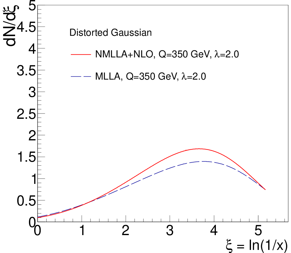
The final expression of the DG parametrisation of the single inclusive distribution of soft hadrons inside gluon and quark jets, Eq. (38), can be obtained summing all its individually-derived NMLLA $+$ NLO^∗-resummed components: the mean multiplicity ${\cal N}(Y,\lambda)$ Eq. (43), the mean peak position $\bar{\xi}(Y,\lambda)$ Eq. (48), the dispersion $\sigma(Y,\lambda)$ Eq. (56), the skewness Eq. $s(Y,\lambda)$ (59), and kurtosis $k(Y,\lambda)$ Eq. (65). In Fig. 3, we display the resulting DG for two different values of the hadronisation parameter $\lambda=1.4$ ( $Y=5.8$ , $Q_{0}=1$ GeV, $\Lambda_{{}_{\rm QCD}}=0.25$ GeV) and $\lambda=2.0$ ( $Y=5.2$ , $Q_{0}=1$ GeV, $\Lambda_{{}_{\rm QCD}}=0.25$ GeV) for a jet of virtuality $Q=350$ GeV and reconstructed jet energy $E=500$ GeV inside a radius cone $\theta=0.7$ . The distribution is compared to the corresponding MLLA predictions with the Fong-Webber results from [22] after setting to zero all terms proportional to $1/Y$ in the same expressions.

The contributions from the set of NMLLA $+$ NLO^∗ corrections to the MLLA DG appear to be quite substantial and decrease for increasing $\lambda$ , since $\lambda$ guarantees the convergence of the perturbative series for $Q_{0}\gg\Lambda_{{}_{\rm QCD}}$ . Physically, for higher values of the shower energy cut-off $Q_{0}$ , the strength of the coupling constant decreases and the probability for the emission of soft gluon bremsstrahlung decreases accordingly, making the multiplicity distribution and the peak position smaller. The difference between the MLLA and NMLLA $+$ NLO^∗ resummed distributions is, as mentioned above, mainly due to running-coupling effects, proportional to $\beta_{1}$ , at large $\xi$ (small $x$ ) which is not unexpected because in this region they are more pronounced due to the $\ln(xE\theta)$ dependence in the denominator of the strong coupling. On the other hand, energy conservation plays a more important role in the hard fragmentation region $x\sim 1$ ( $\xi\sim 0$ ), where the NMLLA $+$ NLO^∗ DG is somewhat suppressed compared with the MLLA DG.

3.3 Multiplicities for the single inclusive $\boldsymbol{D_{g}}$ and $\boldsymbol{D_{q}}$ distributions

In this section we determine the coefficient function involved in Eq. (25a) that provide higher-order corrections to the quark/gluon multiplicity ratio. As shown through Eq. (28), the ${\cal D}^{-}(\omega,\lambda)$ component is negligible and thus the solutions for the gluon and quark single inclusive distributions can be directly obtained from ${\cal D}^{+}$ in the form


$\displaystyle{\cal D}_{q}(\omega,Y,\lambda)\!$	$\displaystyle\!\approx\!$	$\displaystyle\!C_{q}^{g}(\Omega){\cal D}^{+}(\omega,Y,\lambda),\qquad C_{q}^{g}(\Omega)=\frac{P_{qg}(\Omega)}{P_{++}(\Omega)-P_{--}(\Omega)},$	(70a)
$\displaystyle{\cal D}_{g}(\omega,Y,\lambda)\!$	$\displaystyle\!\approx\!$	$\displaystyle\!C_{g}^{g}(\Omega){\cal D}^{+}(\omega,Y,\lambda),\qquad C_{g}^{g}(\Omega)=\frac{P_{++}(\Omega)-P_{qq}(\Omega)}{P_{++}(\Omega)-P_{--}(\Omega)}.$	(70b)

Making use of the expressions (20a)–(20d) and (22a)–(22b), and expanding in $\omega$ results in

\displaystyle C_{q}^{g}(\Omega)\approx\frac{C_{F}}{N_{c}}\left[1+c_{q}^{(0)}\Omega+c_{q}^{(1)}\Omega^{2}+{{\cal{O}}}\left(\Omega^{3}\right)\right],\;C_{g}^{g}(\Omega)\approx 1+c_{g}^{(0)}\Omega+c_{g}^{(1)}\Omega^{2}+{{\cal{O}}}\left(\Omega^{3}\right),

(71)

where the numerical values of the constants, for $n_{f}=5$ quark flavours, read

$\displaystyle c_{q}^{(0)}\!$	$\displaystyle\!=\!$	$\displaystyle\!\frac{a_{1}-b_{1}}{4N_{c}}-\frac{3}{4}\stackrel{{\scriptstyle n_{f}=5}}{{=}}-0.049,$	(72)
$\displaystyle c_{q}^{(1)}\!$	$\displaystyle\!=\!$	$\displaystyle\!\frac{7}{8}+\frac{a_{1}-b_{1}}{16N_{c}}\left(\frac{a_{1}-b_{1}}{N_{c}}-3\right)+\frac{C_{F}}{N_{c}}b_{2}-a_{2}\stackrel{{\scriptstyle n_{f}=5}}{{=}}0.608,$	(73)
$\displaystyle c_{g}^{(0)}\!$	$\displaystyle\!=\!$	$\displaystyle\!-\frac{b_{1}}{4N_{c}}\stackrel{{\scriptstyle n_{f}=5}}{{=}}-0.247,$	(74)
$\displaystyle c_{g}^{(1)}\!$	$\displaystyle\!=\!$	$\displaystyle\!\frac{b_{1}}{16N_{c}^{2}}(b_{1}-a_{1})+\frac{C_{F}}{N_{c}}\left(b_{2}-\frac{5}{8}+\frac{\pi^{2}}{6}\right)\stackrel{{\scriptstyle n_{f}=5}}{{=}}0.045.$	(75)

The $c_{i}^{(0)}$ numerical constants in Eq. (71) were obtained in [4]. Performing the inverse Mellin-transform back to the $x$ -space, or making the equivalent replacement $\Omega\to\frac{\partial}{\partial\xi}+\frac{\partial}{\partial Y}$ , one has


$\displaystyle D_{q}(\xi,Y,\lambda)\!$	$\displaystyle\!\approx\!$	$\displaystyle\!\frac{C_{F}}{N_{c}}\left[1+c_{q}^{(0)}\left(\frac{\partial}{\partial\xi}+\frac{\partial}{\partial Y}\right)+c_{q}^{(1)}\left(\frac{\partial}{\partial\xi}+\frac{\partial}{\partial Y}\right)^{2}\right]D^{+}(\xi,Y,\lambda),$	(76a)
$\displaystyle D_{g}(\xi,Y,\lambda)\!$	$\displaystyle\!\approx\!$	$\displaystyle\!\left[1+c_{g}^{(0)}\left(\frac{\partial}{\partial\xi}+\frac{\partial}{\partial Y}\right)+c_{g}^{(1)}\left(\frac{\partial}{\partial\xi}+\frac{\partial}{\partial Y}\right)^{2}\right]D^{+}(\xi,Y,\lambda),$	(76b)

which in a more compact form can be rewritten as

	$\displaystyle D_{a}(\xi,Y,\lambda)\!$	$\displaystyle\!\approx\!$	$\displaystyle\!\frac{C_{A}}{N_{c}}\left[D^{+}(\xi,Y,\lambda)+c_{A}^{(0)}\left(\frac{\partial D^{+}(\xi,Y,\lambda)}{\partial\xi}+\frac{\partial D^{+}(\xi,Y,\lambda)}{\partial Y}\right)\right.$		(77)
		$\displaystyle\!+\!$	$\displaystyle\!\left.c_{A}^{(1)}\left(\frac{\partial^{2}D^{+}(\xi,Y,\lambda)}{\partial\xi^{2}}+2\frac{\partial^{2}D^{+}(\xi,Y,\lambda)}{\partial\xi\partial Y}+\frac{\partial^{2}D^{+}(\xi,Y,\lambda)}{\partial Y^{2}}\right)\right]$		(78)

for numerical considerations. The first and second derivatives in Eqs. (76a) and (76b) can be evaluated numerically. They provide corrections which are suppressed for the first and second terms of orders ${\cal O}(\sqrt{\alpha_{\rm s}})$ and ${\cal O}(\alpha_{\rm s})$ respectively. In Fig. 4, we compare the quark ( $D_{q}$ ), gluon ( $D_{g}$ ) and parton ( $D^{+}$ ) hadron spectra obtained in the MLLA (left) and NMLLA-NLO^∗ (right) schemes for a jet of virtuality $Q=350$ GeV and hadronisation parameter $\lambda=1.4$ . The NMLLA-NLO^∗ distributions are obtained from the above Eqs. (76a), (76b) and (38), while the MLLA are obtained setting to zero $c_{q}^{(1)}$ and $c_{g}^{(1)}$ in Eqs. (76a) and (76b) respectively and removing the ${{\cal{O}}}\left(\alpha_{\rm s}\right)$ corrections in (38) for $D^{+}(\xi,Y)$ .

A clear difference is observed in the quark and gluon jet initiated distributions given by the colour factor $C_{F}/N_{c}=4/9$ and the role of higher-order corrections which prove more sizable for the NMLLA $+$ NLO^∗ scheme over the whole phase space $0\leq\xi\leq Y$ , as observed in the right panel of Fig. 4. In [4] however, the role of ${{\cal{O}}}\left(\sqrt{\alpha}_{\rm s}\right)$ corrections, proportional to $c_{q}^{(0)}$ and $c_{g}^{(0)}$ in Eqs. (76a) and (76b), was reabsorbed into the inclusive spectrum $D^{+}(\xi,Y)$ through a shift to a slightly different jet energy $E_{A}=E\exp\left(c_{A}^{(0)}\right)$ , which allowed for a direct comparison between the MLLA $D^{+}(\xi,Y)$ and the hadronic energy-momentum spectrum (for a complete review see [10]). Asymptotically ( $Q\to\infty$ ), the solution of the original Eq. (78) has a Gaussian shape near its maximum:

D_{a}(\xi,Q^{2})\approx\frac{C_{A}}{N_{c}}\frac{{\cal N}}{\sigma\sqrt{2\pi}}\exp\left[-\frac{1}{2\sigma^{2}}(\xi-\bar{\xi})^{2}\right],

(79)

normalised by the inverse asymptotic value of the mean multiplicity ratio $r^{-1}=C_{F}/N_{c}$ in a quark jet. The ratio of gluon and quark multiplicities can be recovered by replacing $\omega=0$ ( $\frac{\partial}{\partial\xi}=0$ ) in Eqs. (76a) and (76b), such that, after expanding the result in powers of $\sqrt{\alpha_{\rm s}}$ , one is left with

r=\frac{{\cal N}_{g}}{{\cal N}_{q}}=\frac{N_{c}}{C_{F}}\left(1-r_{1}\gamma_{0}-r_{2}\gamma_{0}^{2}\right),

(80)

where, as a result of the expansion,

	$\displaystyle r_{1}\!\!$	$\displaystyle\!\!=\!\!$	$\displaystyle\!\!c_{q}^{(0)}-c_{g}^{(0)}=\frac{a_{1}}{4N_{c}}-\frac{3}{4},$		(81)
	$\displaystyle r_{2}\!\!$	$\displaystyle\!\!=\!\!$	$\displaystyle\!\!c_{q}^{(1)}-c_{g}^{(1)}-r_{1}c_{q}^{(0)}-\frac{r_{1}}{8N_{c}}\left(a_{1}-\frac{\beta_{0}}{2}\right)=\tilde{a}_{2}-a_{2}+r_{1}\left(\frac{3}{4}-\frac{a_{1}}{8N_{c}}+\frac{\beta_{0}}{16N_{c}}\right),$		(82)

with

\tilde{a}_{2}=\frac{7}{8}+\frac{C_{F}}{N_{c}}\left(\frac{5}{8}-\frac{\pi^{2}}{6}\right).

Notice that up to the order ${{\cal{O}}}\left(\alpha_{\rm s}\right)$ , the multiplicity ratio does not involve corrections proportional to $\beta_{1}$ , which only appear beyond this level of accuracy [20]. Up to the NMLLA order in ${{\cal{O}}}\left(\alpha_{\rm s}\right)$ , Eq. (80) coincides with the expression found in [49], which gives further support to the calculations carried out in our work. A more updated evaluation of the mean multiplicity ratio, including two-loop splitting functions, was given recently in [21].

3.4 Limiting spectrum for the DG parametrisation

The so-called limiting spectrum, $\lambda\to 0$ , implies pushing the validity of the partonic evolution equations down to (non-perturbative) hadronisation scales, $Q_{0}\approx\Lambda_{{}_{\rm QCD}}$ [1]. Such an approach provides a minimal (and successful) approach with predictive power for the measured experimental distributions. We derive here the evolution of the distorted Gaussian moments for this limit which involves formulæ depending only on $\Lambda_{{}_{\rm QCD}}$ as a single parameter.

References

• [1] Y.L. Dokshitzer, V.S. Fadin and V.A. Khoze, Z. Phys. C18 (1983) 37.
• [2] Y.I. Azimov et al., Z. Phys. C27 (1985) 65.
• [3] B. Ermolaev and V.S. Fadin, JETP Lett. 33 (1981) 269.
• [4] Y.L. Dokshitzer et al., Gif-sur-Yvette, France: Ed. Frontières (1991) 274 p. (Basics of); and Rev. Mod. Phys. 60 (1988) 373.
• [5] Y.I. Azimov et al., Zeit. Phys. C31 (1986) 213.
• [6] OPAL Collaboration, M. Akrawy et al., Phys.Lett. B247 (1990) 617.
• [7] CDF Collaboration, T. Aaltonen et al., Phys. Rev. D77 (2008) 092001, arXiv:0802.3182.
• [8] Y.L. Dokshitzer, V.S. Fadin and V.A. Khoze, Zeit. Phys. C15 (1982) 325.
• [9] V.S. Fadin, Yad. Fiz. 37 (1983) 408.
• [10] V.A. Khoze and W. Ochs, Int. J. Mod. Phys. A12 (1997) 2949, hep-ph/9701421.
• [11] R. Pérez Ramos, F. Arleo and B. Machet, Phys. Rev. D78 (2008) 014019, 0712.2212.
• [12] F. Arleo, R. Pérez Ramos and B. Machet, Phys. Rev. Lett. 100 (2008) 052002, 0707.3391.
• [13] V.N. Gribov and L.N. Lipatov, Sov. J. Nucl. Phys. 15 (1972) 438.
• [14] G. Altarelli and G. Parisi, Nucl. Phys. B126 (1977) 298.
• [15] Y.L. Dokshitzer, Sov. Phys. JETP 46 (1977) 641.
• [16] Y.L. Dokshitzer, V.A. Khoze and S. Troian, Z.Phys. C55 (1992) 107.
• [17] A. Capella et al., Phys. Rev. D61 (2000) 074009, hep-ph/9910226.
• [18] F. Cuypers and K. Tesima, Z. Phys. C54 (1992) 87.
• [19] W.E. Caswell, Phys.Rev.Lett. 33 (1974) 244.
• [20] I.M. Dremin and J.W. Gary, Phys. Rept. 349 (2001) 301, hep-ph/0004215.
• [21] P. Bolzoni, B.A. Kniehl and A.V. Kotikov, (2013), 1305.6017.
• [22] C.P. Fong and B.R. Webber, Nucl. Phys. B355 (1991) 54.
• [23] BES Collaboration, W. Dunwoodie et al., Phys.Rev. D69 (2004) 072002, hep-ex/0306055.
• [24] TASSO Collaboration, W. Braunschweig et al., Z. Phys. C41 (1988) 359.
• [25] TASSO Collaboration, W. Braunschweig et al., Z. Phys. C47 (1990) 187.
• [26] TPC/Two Gamma Collaboration, H. Aihara et al., Phys. Rev. Lett. 61 (1988) 1263.
• [27] TOPAZ Collaboration, R. Itoh et al., Phys.Lett. B345 (1995) 335, hep-ex/9412015.
• [28] ALEPH Collaboration, R. Barate et al., Phys.Rept. 294 (1998) 1.
• [29] L3 Collaboration, B. Adeva et al., Phys. Lett. B259 (1991) 199.
• [30] OPAL Collaboration, K. Ackerstaff et al., Eur. Phys. J. C7 (1999) 369, hep-ex/9807004.
• [31] ALEPH Collaboration, D. Buskulic et al., Z. Phys. C73 (1997) 409.
• [32] DELPHI Collaboration, P. Abreu et al., Z. Phys. C73 (1997) 229.
• [33] OPAL Collaboration, G. Alexander et al., Z. Phys. C72 (1996) 191.
• [34] ALEPH Collaboration, A. Heister et al., Eur. Phys. J. C35 (2004) 457.
• [35] OPAL Collaboration, K. Ackerstaff et al., Z. Phys. C75 (1997) 193.
• [36] OPAL Collaboration, G. Abbiendi et al., Eur. Phys. J. C16 (2000) 185, hep-ex/0002012.
• [37] OPAL Collaboration, G. Abbiendi et al., Eur. Phys. J. C27 (2003) 467, hep-ex/0209048.
• [38] G. Altarelli et al., Nucl. Phys. B160 (1979) 301.
• [39] W. Furmanski and R. Petronzio, Zeit. Phys. C11 (1982) 293.
• [40] G. Curci, W. Furmanski and R. Petronzio, Nucl. Phys. B175 (1980) 27.
• [41] S. Albino et al., Eur. Phys. J. C36 (2004) 49, hep-ph/0404287.
• [42] S. Albino, B. Kniehl and G. Kramer, Eur. Phys. J. C38 (2004) 177, hep-ph/0408112.
• [43] S. Albino et al., Phys. Rev. Lett. 95 (2005) 232002, hep-ph/0503170.
• [44] S. Albino et al., Phys. Rev. D73 (2006) 054020, hep-ph/0510319.
• [45] T. Sjostrand, S. Mrenna and P. Skands, JHEP 05 (2006) 026, hep-ph/0603175.
• [46] Y.L. Dokshitzer, D. Diakonov and S.I. Troian, Phys. Rept. 58 (1980) 269.
• [47] A. Vogt, JHEP 1110 (2011) 025, 1108.2993.
• [48] Y.L. Dokshitzer et al., Phys.Lett. B273 (1991) 319.
• [49] I. Dremin and V. Nechitailo, Mod. Phys. Lett. A9 (1994) 1471, hep-ex/9406002.
• [50] S. Sapeta and U.A. Wiedemann, (2008), 0809.4251.
• [51] S. Lupia and W. Ochs, Phys. Lett. B418 (1998) 214, hep-ph/9707393.
• [52] Y.L. Dokshitzer, V.A. Khoze and S. Troian, Int. J. Mod. Phys. A7 (1992) 1875.
• [53] V.A. Khoze, S. Lupia and W. Ochs, Phys.Lett. B386 (1996) 451, hep-ph/9604410.
• [54] S. Albino et al., (2008), 0804.2021.
• [55] S. Albino, Rev. Mod. Phys. 82 (2010) 2489, 0810.4255.
• [56] S. Bethke, Nucl. Phys. Proc. Suppl. 234 (2013) 229, 1210.0325.
• [57] Particle Data Group, J. Beringer et al., Phys.Rev. D86 (2012) 010001.
• [58] D. d’Enterria and R. Pérez-Ramos, Proceeds. Moriond-QCD (2014); arXiv:1408.2865 [hep-ph].