Wetting Boundary Conditions in Phase-Field-Based Simulation of Binary Fluids: Some Comparative Studies and New Development

In the phase-field model, different fluids are distinguished by an order parameter $\phi$, based on which a free energy functional $\mathcal{F}$ is defined as,

$$\mathcal{F}(\phi,\boldsymbol{\nabla}\phi)=\int_{V}\bigg(\Psi(\phi)+\frac{1}{2}\kappa|\boldsymbol{\nabla}\phi|^{2}\bigg)dV+\int_{S}\varphi(\phi_{S})dS,$$

(2.1)

where $\Psi(\phi)$ is the bulk free energy density and takes the following double-well form,

$$\Psi(\phi)=a(\phi^{2}-1)^{2},$$

(2.2)

with $a$ being a constant. This form indicates that $\phi$ varies between $-1$ in one of the fluids and $1$ in the other fluid. (Note that in some works the concentration $C$, instead of the order parameter $\phi$, is used and $C$ varies between $0$ and $1$; but the two formulations using $\phi$ and $C$ can be converted into each other through a linear transformation, thus there are no essential differences between them.) In Eq. (2.1) the second term is the interfacial energy density with $\kappa$ being another constant, and the last term in the surface integral, $\varphi(\phi_{S})$, is the surface energy (SE) density with $\phi_{S}$ being the order parameter on the surface. The specific form of $\varphi(\phi_{S})$ will be discussed later.

By taking the variation of the free energy functional $\mathcal{F}$ with respect to the order parameter $\phi$, one obtains the chemical potential $\mu$ as,

$$\mu=\frac{\delta\mathcal{F}}{\delta\phi}=\frac{d\Psi(\phi)}{d\phi}-\kappa\nabla^{2}\phi=4a\phi(\phi^{2}-1)-\kappa\nabla^{2}\phi.$$

(2.3)

The coefficients $a$ in the bulk free energy and $\kappa$ in the interfacial energy are related to the interfacial tension $\sigma$ and interface width $W$ as  [18],

$$a=\frac{3\sigma}{4W},\quad\kappa=\frac{3\sigma W}{8}.$$

(2.4)

Equivalently, the interfacial tension $\sigma$ and interface width $W$ can be expressed in terms of $a$ and $\kappa$ as,

$$\sigma=\frac{4}{3}\sqrt{2\kappa a},\quad W=\sqrt{\frac{2\kappa}{a}}.$$

(2.5)

By assuming that the diffusion of the order parameter is driven by the gradient of the chemical potential, one has the following evolution equation for $\phi$ [24],

$$\frac{\partial\phi}{\partial t}+(\boldsymbol{u}\cdot\boldsymbol{\nabla})\phi=\boldsymbol{\nabla}\cdot(M\boldsymbol{\nabla}\mu),$$

(2.6)

where $M$ is the mobility (i.e., the diffusion coefficient, which is taken as a constant here). Eq. (2.6) is known as the (convective) Cahn-Hilliard equation (CHE).

Eqs. (2.3) and (2.6) must be supplemented with certain boundary conditions. Here we only discuss the conditions near a wall which are closely related to the wetting and contact line. As seen in Eq. (2.6), the fluid velocity also appears. In this work, we assume the no-slip condition for the fluid velocity $\boldsymbol{u}$ on a wall and focus on the conditions for the PF variables. It should be noted that in PF simulations the interface slip on a wall is allowed because of the diffusion in Eq. (2.6).

Near a solid wall, suitable boundary conditions are required for both the order parameter $\phi$ and the chemical potential $\mu$. Different WBCs differ only in the condition for $\phi$, while they share the same condition for $\mu$. The boundary condition on a surface for the chemical potential $\mu$ is the no-flux condition given by,

$$\boldsymbol{n}_{w}\cdot\boldsymbol{\nabla}\mu|_{S}=\frac{\partial\mu}{\partial n_{w}}\bigg|_{S}=0,$$

(2.7)

where $\boldsymbol{n}_{w}$ denotes the unit normal vector on the surface pointing into the fluid. The different part (i.e., the condition for $\phi$) is described for the five WBCs considered in this work as follows.

In the above, the basics of PF model for binary fluids and five WBCs were introduced. Next, the governing equations and the method for their numerical solution are described. For flows of binary fluids, there are two types of dynamics: the hydrodynamics for fluid flow and the interfacial dynamics. The equation for the latter has been given, i.e., Eq. (2.6) supplemented with Eq. (2.3). For axisymmetric problems, they read,

$$\frac{\partial\phi}{\partial t}+u_{r}\frac{\partial\phi}{\partial r}+u_{z}\frac{\partial\phi}{\partial z}=M\bigg(\frac{\partial^{2}\mu}{\partial r^{2}}+\frac{1}{r}\frac{\partial\mu}{\partial r}+\frac{\partial^{2}\mu}{\partial z^{2}}\bigg),$$

(2.25)

$$\mu=4a\phi(\phi^{2}-1)-\kappa\bigg(\frac{\partial^{2}\phi}{\partial r^{2}}+\frac{1}{r}\frac{\partial\phi}{\partial r}+\frac{\partial^{2}\phi}{\partial z^{2}}\bigg).$$

(2.26)

With the interfacial tension effects modeled by the PF model, the governing equations for the incompressible axisymmetric flow of binary fluids having uniform density and viscosity may be written as,

$$\frac{\partial u_{r}}{\partial r}+\frac{u_{r}}{r}+\frac{\partial u_{z}}{\partial z}=0,$$

(2.27)

$$\begin{split}&\frac{\partial u_{r}}{\partial t}+\bigg(u_{r}\frac{\partial u_{r}}{\partial r}+u_{z}\frac{\partial u_{r}}{\partial z}\bigg)=-\frac{\partial S_{p}}{\partial r}\\ &+\nu\bigg(\frac{\partial^{2}u_{r}}{\partial r^{2}}+\frac{1}{r}\frac{\partial u_{r}}{\partial r}+\frac{\partial^{2}u_{r}}{\partial z^{2}}-\frac{u_{r}}{r^{2}}\bigg)-\phi\frac{\partial\mu}{\partial r},\end{split}$$

(2.28)

$$\begin{split}&\frac{\partial u_{z}}{\partial t}+\bigg(u_{r}\frac{\partial u_{z}}{\partial r}+u_{z}\frac{\partial u_{z}}{\partial z}\bigg)=-\frac{\partial S_{p}}{\partial z}\\ &+\nu\bigg(\frac{\partial^{2}u_{z}}{\partial r^{2}}+\frac{1}{r}\frac{\partial u_{z}}{\partial r}+\frac{\partial^{2}u_{z}}{\partial z^{2}}\bigg)-\phi\frac{\partial\mu}{\partial z},\end{split}$$

(2.29)

where $S_{p}$ is a term similar to the hydrodynamic pressure in single-phase incompressible flow [24]. Note that for simplicity the density and viscosity have been assumed to be uniform and more focus is given to the WBC. To use the notation for 2-D Cartesian coordinates, we replace $(z,r)$ with $(x,y)$. Besides, $(u_{z},u_{r})$ are replaced by $(u,v)$. For 2-D problems (which may be encountered in some of the following studies), the governing equations are simplified. Specifically, they may be obtained by removing the term $M\frac{1}{r}\frac{\partial\mu}{\partial r}$ from Eq. (2.25), the term $-\kappa\frac{1}{r}\frac{\partial\phi}{\partial r}$ from Eq. (2.26), the term $\frac{u_{r}}{r}$ from Eq. (2.27), the two terms, $\nu\frac{1}{r}\frac{\partial u_{r}}{\partial r}$ and $\nu(-\frac{u_{r}}{r^{2}})$, from Eq. (2.28), and the term $\nu\frac{1}{r}\frac{\partial u_{z}}{\partial r}$ from Eq. (2.29).

In the hybrid lattice-Boltzmann finite-difference method [22], the LBM is employed to simulate the hydrodynamics, described by the Navier-Stokes equations (NSEs, specifically, Eqs. (2.27), (2.28) and (2.29) for axisymmetric problems), whereas the equation for the interface motion (the CHE, Eq. (2.6)), is solved by the finite-difference method for spatial discretization and the $4^{th}-$order Runge-Kutta method for time marching. The details of this hybrid method can be found in the Ref.  [22] and will not be repeated. Here more attention is paid to the specific implementations of different WBCs. We note that there are different choices for several components in the hybrid method in [22]. The present work uses the multiple-relaxation-time (MRT) collision model for LBM, the centered formulation for the forcing terms, and the isotropic discretization based on D2Q9 velocity model (i.e., the iso scheme in  [22]) to evaluate the spatial gradients of the PF variables.

The domain of simulation is a rectangle specified by $0\leq x\leq L_{x},\ 0\leq y\leq L_{y}$. It is discretized into $N_{x}\times N_{y}$ uniform squares of side length $h$, thus, $L_{x}=N_{x}h$ and $L_{y}=N_{y}h$. The distribution functions in LBM and the discrete phase-field variables, $\phi_{i,j}$ and $\mu_{i,j}$, are both located at the centers of the squares (like the cell centers in the finite-volume method). The indices $(i,j)$ for the bulk region (i.e., within the computational domain) are $1\leq i\leq N_{x},\ 1\leq j\leq N_{y}$.

As seen in Section 2.2, all WBCs (except CI) involve the enforcement of the normal gradient of the order parameter $\phi$ on the wall. Consider the case with the lower side of a rectangle being a wall with a given contact angle $\theta_{w}$. The enforcement of $\phi$’s normal gradient is realized by adding a ghost layer of squares having the same size as those in the bulk region, the centers of which are $h/2$ below the wall with the index $j=0$. Although the normal gradient of $\phi$ is not directly enforced in CI, it also specifies the value of $\phi$ in the ghost layer.

When LinSE is used, after discretization, Eq. (2.12) becomes,

$$\frac{\phi_{i,1}-\phi_{i,0}}{h}=-\frac{2}{W}\tilde{\omega},$$

(2.30)

giving the order parameter in the ghost layer,

$$\phi_{i,0}=\phi_{i,1}+\frac{2}{W/h}\tilde{\omega}=\phi_{i,1}+\frac{2}{\tilde{W}}\tilde{\omega},$$

(2.31)

where $\tilde{W}=W/h$ is the dimensionless interface width (i.e., $W$ measured in the grid size $h$). Similarly, when CubSE is used, one finds,

$$\phi_{i,0}=\phi_{i,1}+\frac{2}{\tilde{W}}\cos\theta_{w}(1-\phi_{S}^{2}),$$

(2.32)

and for SinSE one has,

$$\phi_{i,0}=\phi_{i,1}+\frac{2}{\tilde{W}}\cos\theta_{w}\bigg[\frac{\pi}{3}\cos\bigg(\frac{\pi}{2}\phi_{S}\bigg)\bigg].$$

(2.33)

When Geom is used, one has,

$$\phi_{i,0}=\phi_{i,1}+\tan\bigg(\frac{\pi}{2}-\theta_{w}\bigg)|\boldsymbol{t}_{w}\cdot\boldsymbol{\nabla}\phi|h.$$

(2.34)

It is seen that, unlike Eq. (2.31), Eqs. (2.32), (2.33), and (2.34) contain additional unknowns which must be found by some means. In Eq. (2.32) and (2.33), $\phi_{S}$ is the order parameter on the wall. For $\theta_{w}\neq 90^{\circ}$ ($\cos\theta_{w}\neq 0$), when CubSE is used, $\phi_{S}$ can be found from the following equation (derived by assuming a quadratic profile for $\phi$ as a function of the coordinate normal to the wall; see [20] for more details),

$$\phi_{S}^{2}+\frac{8}{3q}\phi_{S}-1+\frac{8\phi_{i,1}-(\phi_{i,2}-\phi_{i,1})}{-3q}=0,\quad\textrm{with}\quad q=\frac{2}{\tilde{W}}\cos\theta_{w},$$

(2.35)

and when SinSE is used, $\phi_{S}$ satisfies,

$$8\phi_{S}-q\pi\cos\bigg(\frac{\pi}{2}\phi_{S}\bigg)-(9\phi_{i,1}-\phi_{i,2})=0.$$

(2.36)

Note that Eq. (2.35) has two solutions and it is necessary to discard one of them that is not suitable (e.g., out of the range of $\phi$). The solution of Eq. (2.36) may be found by Newton’s method with the initial guess of $\phi_{S}$ obtained from a simple linear extrapolation as $\phi_{S}=1.5\phi_{i,1}-0.5\phi_{i,2}$. For $\theta_{w}=90^{\circ}$ ($\cos\theta_{w}=0$), it is straightforward to find from Eq. (2.32) or Eq. (2.36) that $\phi_{i,0}=\phi_{i,1}$. For Geom, Eq. (2.34) contains the tangential component of $\phi$’s gradient on the wall, $\boldsymbol{t}_{w}\cdot\boldsymbol{\nabla}\phi|_{S}$, and it is evaluated by the following extrapolation scheme,

$$\boldsymbol{t}_{w}\cdot\boldsymbol{\nabla}\phi|_{S}=1.5\boldsymbol{t}_{w}\cdot\boldsymbol{\nabla}\phi|_{i,1}-0.5\boldsymbol{t}_{w}\cdot\boldsymbol{\nabla}\phi|_{i,2},$$

(2.37)

where the tangential gradients on the RHS are calculated by the $2^{nd}$-order central difference scheme, for example,

$$\boldsymbol{t}_{w}\cdot\boldsymbol{\nabla}\phi|_{i,1}=\frac{\partial\phi}{\partial t_{w}}\bigg|_{i,1}=\frac{\phi_{i+1,1}-\phi_{i-1,1}}{2h}.$$

(2.38)

It is noted that in [12] Eq. (2.34) was applied only in the interfacial region (specified by $0.001<C_{i,1}<0.999$). Since away from the interface the gradient of the order parameter is negligible, it is acceptable to apply Eq. (2.34) everywhere along the layer near the wall (which is adopted in this work).

In the CI-based WBC, the values of $\phi$ in the ghost layer are found by drawing the respective characteristic lines (contours of $\phi$) from the centers of the squares in the ghost layer, which intersect the wall at the given contact angle $\theta_{w}$, and linearly interpolating the values of $\phi$ at the intersection points of such characteristic lines and the layer nearest to the wall (i.e., the layer with the index $j=1$). The illustration of the idea may be found in Fig. 4 of [28] and the specific formulas to obtain $\phi_{i,0}$ were given in [28] as well. Both Geom and CI aim to enforce exactly the microscopic contact angle right on the wall directly (of course, with certain approximations embedded in the numerical evaluations of derivatives or in the extrapolations and interpolations). Thus, it is expected that they would likely give similar results.

Once the order parameter in the ghost layer below the wall is specified according to the respective formulas, the WBC is implemented completely. For a wall along some other directions, the formulas for different WBCs are similar (only some changes to the indices are required). For conciseness they are not given here.

In [7, 45], an additional parameter was introduced to control the speed of the establishment of local equilibrium on the wall. As pointed by Yue and Feng [45], the additional parameter may be explored as a phenomenological parameter to match the simulation results with experimental ones. Here we propose the inclusion of an additional simple procedure in the implementation of the WBC which serves a similar purpose. This additional step is also partly inspired by the implementation of the contact angle hysteresis (CAH) model by Ding and Spelt [13]. Specifically, this step is about the update of the value of $\phi$ in the ghost layer. We still use the lower wall to illustrate the details. In the above, the equations to obtain $\phi_{i,0}$ have been presented (for different WBCs the equation differs, for instance, Eq. (2.32) is from CubSE). For concreteness, we take CubSE as an example: Eq. (2.32) is employed to update $\phi_{i,0}$ at every time step (or sub-step), and the values of $\phi_{i,0}$ in previous steps are not used at all. By contrast, for the CAH model implemented according to [13], when the local contact angle is between the advancing and receding contact angles, $\phi_{i,0}$ is not updated (i.e., keeps its value in previous step) so that the hysteresis effects are taken into account. For convenience, denote the value of $\phi_{i,0}$ at the new step (or sub-step) in case of no slip (i.e., completely hysteretic) as $\phi_{i,0}^{hy}$ (equal to its value in previous step or sub-step) and that in case of full slip as $\phi_{i,0}^{sl}$ (its value given by Eq. (2.32)). Now we propose the following procedure to calculate $\phi_{i,0}$ at each new time step (or sub-step),

$$\phi_{i,0}=\phi_{i,0}^{hy}+r_{wr}(\phi_{i,0}^{sl}-\phi_{i,0}^{hy})=r_{wr}\phi_{i,0}^{sl}+(1-r_{wr})\phi_{i,0}^{hy},$$

(2.39)

where $r_{wr}$ ($0\leq r_{wr}\leq 1$) is a newly introduced parameter to control the rate of relaxation on the wall, and $\Delta\phi_{i,0}=\phi_{i,0}^{sl}-\phi_{i,0}^{hy}$ corresponds to the change of $\phi_{i,0}$ in case of full slip. It is easy to see that $r_{wr}=0$ corresponds to the case of no slip and $r_{wr}=1$ corresponds to the case of full slip. As compared to the relevant equations in [7] and [45], Eq. (2.39) is more simple and does not involve the discretization of time derivatives. Besides, the meaning of the new parameter $r_{wr}$ is obvious (i.e., the weight to control how much slip is allowed).

Before presenting the results, we first introduce the characteristic quantities and dimensionless numbers, as well as some common setups for the problems to be studied. In each problem, we study a drop with a radius $R$ or a liquid column with a height or diameter $H$, and $R$ or $H$ is chosen to be the characteristic length $L_{c}$ (for convenience, we use $R$ in the following general formulas). The (constant) density is selected as the characteristic density $\rho_{c}$. The interfacial tension is $\sigma$ and the kinematic viscosity is $\nu$ (thus, the dynamic viscosity is $\eta=\rho_{c}\nu$). As in some previous works [27, 22], here we use the following characteristic velocity $U_{c}$,

$$U_{c}=\frac{\sigma}{\rho_{c}\nu},$$

(3.1)

leading to a characteristic time $T_{c}$ given by,

$$T_{c}=\frac{L_{c}}{U_{c}}=\frac{R\rho_{c}\nu}{\sigma}.$$

(3.2)

For problems on drop motion, one may derive another set of characteristic quantities (which are typically used in inviscid dynamics [15]),

$$U_{c,\textrm{inv}}=\sqrt{\frac{\sigma}{\rho_{c}R}},\quad T_{c,\textrm{inv}}=\frac{L_{c}}{U_{c,\textrm{inv}}}=\frac{R}{U_{c,\textrm{inv}}}=\sqrt{\frac{\rho_{c}R^{3}}{\sigma}}.$$

(3.3)

All other quantities of length, time and velocity below are scaled by $L_{c}$, $T_{c}$ and $U_{c}$ by default (sometimes $T_{c,\textrm{inv}}$ and $U_{c,\textrm{inv}}$ are used instead of $T_{c}$ and $U_{c}$). There are two important physical parameters in drop problems: (1) the capillary number, which reflects the ratio of the viscous force over the interfacial tension force, and with the above definition of $U_{c}$, is found to be always unity,

$$Ca=\frac{\rho_{c}\nu U_{c}}{\sigma}=1,$$

(3.4)

(2) the Reynolds number, which reflects the ratio of the inertial force over the viscous force and is found to be (if $U_{c}$ is used),

$$Re=\frac{U_{c}R}{\nu}=\frac{\sigma}{\rho_{c}\nu}\frac{R}{\nu}=\frac{\sigma R}{\rho_{c}\nu^{2}}.$$

(3.5)

It is noted that based on $U_{c,\textrm{inv}}$ one may define another capillary number and Reynolds number as [39],

$$Ca_{\sigma}=\frac{\rho_{c}\nu U_{c,\textrm{inv}}}{\sigma}=\frac{1}{\sqrt{Re}},\quad Re_{\sigma}=\frac{U_{c,\textrm{inv}}R}{\nu}=\sqrt{Re}.$$

(3.6)

In addition, the Ohnesorge number $Oh$ is also often used for drop dynamics [44]. If the drop radius (instead of the drop diameter in [44]) is used, $Oh$ reads,

$$Oh=\frac{\rho_{c}\nu}{\sqrt{\rho_{c}\sigma R}},$$

(3.7)

which is found to be related to the other dimensionless numbers as $Oh=1/\sqrt{Re}=1/Re_{\sigma}=Ca_{\sigma}$.

In PF simulations, there are two additional parameters: (1) the Cahn number, defined to be the ratio of interface width over the characteristic length,

$$Cn=\frac{W}{L_{c}},$$

(3.8)

(2) the Peclet number, measuring the relative magnitude of convection over diffusion in the CHE,

$$Pe=\frac{U_{c}L_{c}^{2}}{M\sigma}.$$

(3.9)

We note that Yue et al. [47] studied the convergence of numerical results by PF simulations towards the sharp-interface limit and proposed the use of an alternative parameter $S$ (instead of $Pe$) defined by,

$$S=\frac{\sqrt{M\nu}}{L_{c}},$$

(3.10)

which reflects the diffusion length scale at the contact line (relative to the characteristic length) [47] and could be more appropriate for problems involving contact lines. In this work both $Pe$ and $S$ are provided. In the literature, there are some investigations and discussions on how to choose $Cn$ and $Pe$ (or $S$) to obtain reliable results for different problems [24, 47]. We will also carry out some studies in this aspect for one of the problems below (drop dewetting). It is noted that the present definition of Cahn number differs from some others because of different definitions of the interface width. In [47, 14] the interface width $\varepsilon$ is related to the present one as $\varepsilon=W/(2\sqrt{2})$ whereas in [41] the interface width $\xi$ is related to $W$ as $\xi=W/\sqrt{2}$.

In all simulations, the lower side is the symmetric axis on which the symmetric boundary conditions are applied, and the upper side is a stationary solid wall with wall boundary conditions applied. The wettability of the upper wall and the boundary types of the left and right sides differ in different problems, and they will be stated later individually. The simulations are performed in the temporal range $0\leq t\leq t_{e}$, where $t_{e}$ denotes the time (measured in $T_{c}$ by default, or in $T_{c,\textrm{inv}}$ when specified so) at the end of the simulation. Suppose the characteristic length $L_{c}$ is discretized by $N_{L}$ uniform segments and the characteristic time $T_{c}$ (as defined in Eq. (3.2)) is discretized by $N_{t}$ uniform segments, then one has the grid size $h$ and time step $\delta_{t}$ as follows,

$$h=\frac{L_{c}}{N_{L}},\quad\delta_{t}=\frac{T_{c}}{N_{t}}.$$

(3.11)

Recall that the domain of size $L_{x}\times L_{y}$ is discretized into $N_{x}\times N_{y}$ uniform squares ($L_{x}=N_{x}h$ and $L_{y}=N_{y}h$), one has $h=L_{c}/N_{L}=L_{x}/N_{x}=L_{y}/N_{y}$.

In all problems, we are concerned about the centroid (average) velocity (of the drop or liquid column) in the $x$-direction. Take the drop under the cylindrical geometry as an example: the average velocity $\overline{U}_{d}(t)$ may be calculated by,

$$\overline{U}_{d}(t)=\frac{\int_{V}N(\phi)u(t)d\Omega}{\int_{V}N(\phi)d\Omega}\approx\frac{\sum_{i,j}y_{i,j}u_{i,j}(t)N(\phi_{i,j})}{\sum_{i,j}y_{i,j}N(\phi_{i,j})},$$

(3.12)

where $V$ denotes the domain, $d\Omega(=2\pi rdrdz)=2\pi ydydx\approx(2\pi h^{2})y_{i,j}$ under the cylindrical geometry, and the function $N(\phi)$ is defined by,

$$N(\phi)=\left\{\begin{array}[]{cl}1&\quad\textrm{if}\quad\phi>0\\ 0&\quad\textrm{if}\quad\phi\leq 0\end{array}\right..$$

(3.13)

For a liquid column under the same geometry, the centroid (average) velocity (denoted by $v_{\textrm{lc}}$) is also calculated by Eq. (3.12) (under 2-D geometry, the formula is more simple because $d\Omega=dxdy$). In addition, from Eq. (2.23), a local dynamic contact angle $\theta_{d,l}$ (in degree ^∘) may be calculated from the local gradients of the order parameter on the wall as,

$$\theta_{d,l}=\frac{180^{\circ}}{\pi}\bigg(\frac{\pi}{2}-\arctan\frac{-\frac{\partial\phi}{\partial n_{w}}}{|\frac{\partial\phi}{\partial t_{w}}|}\bigg).$$

(3.14)

It should be noted that far away from the interfaces $|\frac{\partial\phi}{\partial t_{w}}|$ may become zero and Eq. (2.23) is thus for the interfacial region only. In the results presented below, the interfacial region is specified by the following conditions: $|\frac{\partial\phi}{\partial t_{w}}|*h>0.1$ and $-0.998\leq\phi\leq 0.998$; outside this region, we set $\theta_{d,l}=0$. Near the interface (where $\phi=0$) the dynamic contact angle on the wall is denoted simply as $\theta_{d}$. Besides, the dynamic contact angle near the wall (obtained one grid away from the wall) is denoted as $\theta_{d,NW}$. These two dynamic contact angles and the nodes involved in their calculation are illustrated in Fig. 1 for the case with a wall on the lower side.

First, we study the static contact angle of a drop on a homogeneous wall. Specifically, we investigate whether a drop having an initial shape corresponding to an initial contact angle of $\theta_{i}$ and also in touch of a wall with the wettability specified by an contact angle $\theta_{w}$ ($\theta_{w}\neq\theta_{i}$) can evolve to reach an equilibrium state with a contact angle equal to $\theta_{w}$. In this study (and that on drop dewetting), the other common setups besides those given above are as follows. Both the left and right sides are stationary walls. The contact angle of the left wall is $\theta_{w}$ which may take different values, and those of the upper and right walls are $90^{\circ}$ (which is not quite important because the drop does not touch them). The initial position of the drop center (actually the center of the circle of which the middle cross section of the drop is a part) is $(x_{c},y_{c})$ with $y_{c}=0$ (as required by the fact that the lower side is a line of symmetry). From simple geometrical relations, the initial (given) contact angle $\theta_{i}$ (in degree ^∘) corresponding to the initial drop shape is related to $x_{c}$ as,

$$\theta_{i}=\frac{180^{\circ}}{\pi}\times\left\{\begin{array}[]{cl}(\pi-\arccos\frac{x_{c}}{R})&\quad\textrm{if}\quad x_{c}>0\\ \arccos\frac{-x_{c}}{R}&\quad\textrm{if}\quad x_{c}\leq 0\end{array}\right..$$

(3.15)

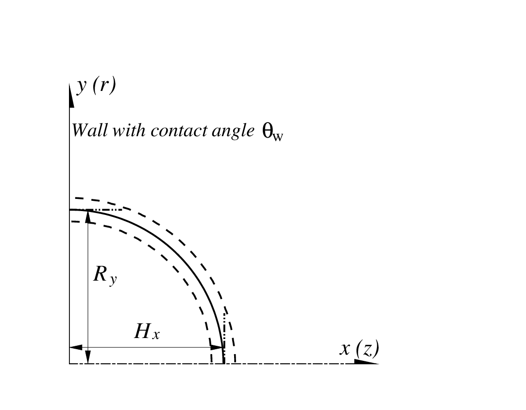
In this work, we fix the initial drop center as $(x_{c},y_{c})=(0,0)$, giving an initial contact angle $\theta_{i}=90^{\circ}$. The domain size is $L_{x}\times L_{y}=4\times 4$. Figure 2 illustrates the basic setup and also the initial condition for the study of static contact angle (and also for drop dewetting). Note that only the region near the drop is shown, and the upper and right walls are not included in Fig. 2. We monitor the drop height on the $x-$axis $H_{x}=H_{x}(t)$ and the drop radius on the left wall $R_{y}=R_{y}(t)$ (i.e., the radius of the circle on the wall formed by the contact line). The illustrations of $H_{x}$ and $R_{y}$ are also given in Fig. 2. If the drop shape (in the middle cross section) is part of a circle (which is reasonable if inertial effects are relatively small or negligible), the instantaneous contact angle $\theta_{d,\textrm{sf}}=\theta_{d,\textrm{sf}}(t)$ (obtained by fitting the drop shape at $t$, also in degree ^∘) may be deduced from $H_{x}$ and $R_{y}$ as (using the relation similar to Eq. (3.15))  [19],

$$\theta_{d,\textrm{sf}}=\frac{180^{\circ}}{\pi}\bigg(\pi-\arccos\bigg(\frac{1-k_{r}^{2}}{1+k_{r}^{2}}\bigg)\bigg),\quad\textrm{with}\quad k_{r}=R_{y}/H_{x}.$$

(3.16)

Even if the inertial effect plays a role during the evolution, the above assumption for calculating $\theta_{d,\textrm{sf}}$ is well satisfied at the end ($t=t_{e}$) when the static equilibrium is almost reached.

For this study, the physical parameters are $Re=1000$ ($Oh=0.032$), $Ca=1$, and the numerical parameters are $Cn=0.2$, $Pe=5000$ ($S=0.014$), $N_{L}=20$ ($\tilde{W}=4$), $N_{t}=80$, $t_{e}=500$ (large enough to ensure that $\theta_{d,\textrm{sf}}$ becomes almost constant). The focus of this problem is the final state and the temporal evolution is not concerned. Figure 3 compares the equilibrium contact angle $\theta_{d,\textrm{sf}}^{eq}$ (as obtained from $H_{x}$ and $R_{y}$ using Eq. (3.16) at $t=500$) under several given contact angles ($\theta_{w}=45^{\circ}$, $60^{\circ}$, $75^{\circ}$, $105^{\circ}$, $120^{\circ}$, and $135^{\circ}$) of the left wall by using LinSE, CubSE, SinSE, Geom and CI. It is seen that for each $\theta_{w}$ upon reaching equilibrium all the WBCs can give a contact angle that agrees reasonably well with the given one. For $\theta_{w}$ being far away from $90^{\circ}$, the deviations become somewhat larger, but the numerical ones are still fairly close to the theoretical values. Thus, the differences between the five WBCs, if any, should mainly exist under dynamic situations.

Next, we will study some dynamic problems. This first is the steady motion of a liquid column inside a cylindrical tube with a diameter $H$ driven by a Poiseuille flow. The parabolic Poiseuille velocity profile is imposed on the left and right sides (inlet and outlet). The average of this Poiseuille velocity profile is $\overline{V}$. This is also an axisymmetric problem and can be simplified as a pseudo 2-D problem. Again, the symmetry about the axis ($y=0$) allows us to use only the upper half domain ($0\leq y\leq 0.5H$) in simulation. The characteristic length is the tube diameter ($L_{c}=H$). Figure 4 illustrates the setup for this problem. Initially, the liquid column has a width of $W_{\textrm{lc}}=2H$ and its center is located at $(1.5H,0)$. The (static) contact angle of the tube wall (the upper wall in Fig. 4) is $\theta_{w}=98^{\circ}$. On the left and right sides, inlet and outlet boundary conditions are employed for the distribution functions (in the ghost layers which are not involved in LBM calculations): the equilibrium parts are calculated from the given parabolic Poiseuille velocity profile whereas the non-equilibrium parts are obtained from bounce-back rules. For the PF variables, periodic boundary conditions are employed on these two sides. Driven by the imposed Poiseuille flow, the liquid column is gradually accelerated towards the right end and achieves a steady motion after certain time. In most of the cases studied here, the length of the domain is $L_{x}=5H$, which is long enough for the liquid column to achieve the steady state (note in some cases it is extended up to $L_{x}=15H$ to satisfy this requirement). To reach the steady state, the simulation time ranges from $3$ to $10$ $T_{c,\textrm{inv}}$ depending on the specific parameters like the average velocity $\overline{V}$ and the relaxation parameter $r_{wr}$ in the boundary condition. For this study, the physical parameters are $Re=100$ ($Oh=0.1$), $Ca=1$, and the numerical parameters are $Cn=0.125$, $Pe=5000$ ($S=0.014$), $N_{L}=32$ ($\tilde{W}=4$). The temporal discretization parameter $N_{t}$ was varied from $320$ to $3200$ depending on the average velocity $\overline{V}$.

In this problem, we are only concerned about the steady state, in which the liquid column moves at a constant speed (just equal to $\overline{V}$). Based on $\overline{V}$, one can define another capillary number as,

$$Ca_{\overline{V}}=\frac{\rho_{c}\nu_{A}\overline{V}}{\sigma},$$

(3.17)

where $\nu_{A}$ is the kinematic viscosity of the liquid column. We focus on the advancing interface on the right. It is noted that there is no obvious difference in the advancing interfaces between a liquid column of a finite length (which is long enough to keep the advancing and receding interfaces apart during the motion) and that of an infinite length when the steady state is reached. This allows us to compare the current simulations with those reported by Fermigier and Jenffer [17], who studied the motion of a liquid-liquid interface inside a tube. Two key dimensionless parameters were mentioned in their experiments, namely, the capillary number ($Ca_{\overline{V}}$ defined here) and the (dynamic) viscosity ratio $r_{\eta}$ (defined as $r_{\eta}=\eta_{A}/\eta_{B}$ with $\eta_{A}$ and $\eta_{B}$ being the dynamic viscosities of the displacing liquid and the displaced liquid, respectively). Here we focus on one set of experimental data reported in their work with a viscosity ratio $r_{\eta}=0.9$. For simplicity the viscosity ratio in our simulations is set to be $r_{\eta}=1$ (without introducing large deviations). The advancing contact angle $\theta_{A}$ is obtained by least-square fitting the middle part ($0\leq y\leq 0.25H$) of the advancing interface with a circle. It was found that the velocity of the liquid column became steady relatively fast (the time taken depends on the capillary number). The steady velocity of the liquid column obtained numerically by using Eq. (3.12) matched the average of the imposed Poiseuille flow ($\overline{V}$) very well for all capillary numbers and WBCs. At the same time, it took longer time for $\theta_{A}$ to become steady: in fact, it was found that $\theta_{A}$ fluctuates around some value for each $Ca_{\overline{V}}$ even after long time and the oscillation amplitude decreases with increasing $Ca_{\overline{V}}$. Fortunately, the fluctuations remained small (around $2^{\circ}$ for the smallest $Ca_{\overline{V}}$ considered). For convenience, the value of $\theta_{A}$ at the end of simulation is taken. Besides $\theta_{A}$, we also looked into the dynamic contact angle on the upper wall (at $y=0.5H$ near the advancing interface where $\phi=0$), $\theta_{d}^{\textrm{rig}}$, and the dynamic contact angle near the upper wall, $\theta_{d,NW}^{\textrm{rig}}$, obtained one grid away from the wall (at $y=0.5H-h$) near the interface.

It was observed that when the full slip condition was used (i.e. $r_{wr}=1$), different WBCs gave almost the same results for both $v_{\textrm{lc}}$ and $\theta_{A}$ even though the dynamic contact angles on and near the wall ($\theta_{d}^{\textrm{rig}}$ and $\theta_{d,NW}^{\textrm{rig}}$) were slightly different (the results given by LinSE differed from the others the most). For conciseness, the detailed results are not shown here. In addition, the role of wall energy relaxation was also studied for two WBCs (CubSE and Geom). Figure 5 shows the variations of the advancing contact angle $\theta_{A}$ (obtained by the least-square fitting of the middle portion of the interface as mentioned above) with the capillary number $Ca_{\overline{V}}$ from both the present simulations with different WBCs and different values of the relaxation parameter $r_{wr}$, and the experimental measurements by Fermigier and Jenffer [17]. It is seen the prediction by simulations using CubSE with $r_{wr}=1$ differ from the experimental data significantly. By properly adjusting the relaxation parameter $r_{wr}$, both CubSE and Geom can give very good predictions that match closely the experimental data over a wide range of capillary number. It is noted that the substantial improvement due to proper wall energy relaxation has been reported by Yue and Feng [45] in the study of a similar problem and by Carlson et al. [7] in the study of very fast drop spreading. For the two WBCs (CubSE and Geom), the main difference seems to be only in the suitable value of relaxation parameter $r_{wr}$ (which differ slightly: $3.5\times 10^{4}$ for CubSE and $3.2\times 10^{4}$ for Geom). The agreement becomes not so good when $Ca_{\overline{V}}$ is so large that $\theta_{A}$ is near $180^{\circ}$. This may be caused by the fact that when $\theta_{A}$ is near $180^{\circ}$ (wetting failure is about to occur) it is difficult to accurately fit the interface with an arc, and large deviations exist in $\theta_{A}$ obtained by the least-square fitting. Based on the above observations, it may be concluded that for mechanically driven two-phase flows it is not quite sensitive on which WBCs to be used if the feature of bulk flow (away from the wall) is concerned.

The second dynamic problem has a different driving mechanism: in stead of an imposed flow, a given wettability gradient (WG) is applied to drive a liquid column. Specifically, we consider a liquid column inside a channel composed of two horizontal flat plates (located at $y=-0.5H$ and $y=0.5H$) under 2-D geometry and also another one inside a cylindrical tube (with a diameter $H$). The 2-D case was used as a validation case recently in [23] and a similar problem was investigated in [16]. The problem under cylindrical geometry is studied here for the first time (as far as we know), and it can also be simplified as a pseudo 2-D problem. For completeness, we briefly reintroduce the problem setup here. Under either 2-D or cylindrical geometry, the problem is symmetric about the middle horizontal line $y=0$, thus only the upper half ($0\leq y\leq 0.5H$) is used. The characteristic length is chosen to be the channel height or the tube diameter ($L_{c}=H$). Figure 6 illustrates the problem setup. Note only part of the upper half (the region near the liquid column) is shown in Fig. 6 because of the relatively large domain length ($L_{x}\gg H$). Initially, the liquid column has a (nominal) width of $W_{\textrm{lc}}=4H$ (the distance between the two three-phase points (TPPs) in $x-$direction is roughly $W_{\textrm{lc}}$). The $x-$coordinate of the middle point between the two TPPs is $x^{\textrm{mid}}=3.5H$, giving the $x-$coordinates of the left and right TPPs as $x^{\textrm{lef}}=1.5H$ and $x^{\textrm{rig}}=5.5H$. In the region $x>x^{\textrm{mid}}$ the wettability of the wall is specified by a (static) contact angle $\theta_{w}^{\textrm{rig}}$, and for $x\leq x^{\textrm{mid}}$ the contact angle is $\theta_{w}^{\textrm{lef}}$ ($\theta_{w}^{\textrm{lef}}>\theta_{w}^{\textrm{rig}}$). The initial right and left interface shapes are specified to be two arcs that intersect the wall with angles $\theta_{w}^{\textrm{rig}}$ and $\theta_{w}^{\textrm{lef}}$, respectively. Both the right and left parts of the wall are assumed to be geometrically smooth and have no hysteresis. Because of the difference in the contact angle (which results in a stepwise WG), the liquid column is driven by the interfacial tension forces to move right (i.e., towards the more lyophilic part). Boundary conditions for a stationary wall are applied on the upper side ($y=0.5H$). Periodic boundaries are assumed on the left and right sides. The length of the domain is $L_{x}=20H$. To ensure that the liquid column is always under the action of the WG, the position of the middle point $x^{\textrm{mid}}=(x^{\textrm{lef}}+x^{\textrm{rig}})/2$ is monitored at each step and the wettability distribution is updated based on $x^{\textrm{mid}}$ to maintain the WG.

After certain time, the liquid column gradually reaches a steady state, which indicates a balance between the interfacial tension forces and the viscous resistances. Note that the dynamic contact angle on the wall $\theta_{d}$ could be equal or not equal to the static contact angle $\theta_{w}$, depending on the WBC used. By assuming that the velocity across the channel takes a parabolic Poiseuille velocity profile (which should be acceptable if the regions covered by the interfaces occupy only a small portion of the whole domain), Esmaili et al. [16] obtained an approximate analytical solution for the evolution of the centroid velocity of the liquid column $v_{\textrm{lc}}$ under 2-D geometry as (the equation given here has been simplified for cases with uniform density $\rho_{c}$),

$$v_{\textrm{lc}}=\frac{\sigma H[2(\cos\theta_{d}^{\textrm{rig}}-\cos\theta_{d}^{\textrm{lef}})]}{12\rho_{c}[\nu_{A}W_{\textrm{lc}}+\nu_{B}(L_{x}-W_{\textrm{lc}})]}(1-e^{-t/t_{s}}),$$

(3.18)

with $t_{s}=H^{2}L_{x}/[12(\nu_{A}W_{\textrm{lc}}+\nu_{B}(L_{x}-W_{\textrm{lc}}))]$ where $\nu_{B}$ is the kinematic viscosity of the fluid outside the liquid column, and $\theta_{d}^{\textrm{rig}}$ and $\theta_{d}^{\textrm{lef}}$ are the dynamic contact angles at the right and left TPPs (note it is not clear whether the dynamic contact angles were calculated by Esmaili et al. [16] in the same way as described above). Here we have further derived the formula under cylindrical geometry based on similar assumptions, which reads,

$$v_{\textrm{lc}}=\frac{\sigma H(\cos\theta_{d}^{\textrm{rig}}-\cos\theta_{d}^{\textrm{lef}})}{8\rho_{c}[\nu_{A}W_{\textrm{lc}}+\nu_{B}(L_{x}-W_{\textrm{lc}})]}(1-e^{-t/t_{s}}),$$

(3.19)

with $t_{s}=H^{2}L_{x}/[32(\nu_{A}W_{\textrm{lc}}+\nu_{B}(L_{x}-W_{\textrm{lc}}))]$. From the above equations, it is seen that as $t/t_{s}\rightarrow\infty$ the velocity approaches a constant value $V_{\textrm{lc}}$ for either the 2-D or axisymmetric case, specifically,

$$V_{\textrm{lc}}^{\textrm{2D}}=\frac{\sigma H[2(\cos\theta_{d}^{\textrm{rig}}-\cos\theta_{d}^{\textrm{lef}})]}{12\rho_{c}[\nu_{A}W_{\textrm{lc}}+\nu_{B}(L_{x}-W_{\textrm{lc}})]},\quad V_{\textrm{lc}}^{\textrm{Axisym}}=\frac{\sigma H(\cos\theta_{d}^{\textrm{rig}}-\cos\theta_{d}^{\textrm{lef}})}{8\rho_{c}[\nu_{A}W_{\textrm{lc}}+\nu_{B}(L_{x}-W_{\textrm{lc}})]}.$$

(3.20)

It must be noted that in the derivation of Eqs. (3.18) and (3.19) it is assumed that both dynamic contact angles, $\theta_{d}^{\textrm{rig}}$ and $\theta_{d}^{\textrm{lef}}$, are constant. This assumption might not always be true. However, even if they are time-dependent, usually they should vary in a small range for the parameters considered here. In that case, one may express the dynamic contact angle as,

$$\theta_{d}(t)=\theta_{d}(0)[1+\epsilon(t)],\quad\textrm{where}\quad|\epsilon(t)|\ll 1.$$

(3.21)

Then Eqs. (3.18) and (3.19) may be obtained when the leading order terms are used.

For this problem, all the five WBCs were tried (without wall energy relaxation, i.e., $r_{wr}=1$). The common parameters are $Re=100$ ($Oh=0.1$), $r_{\nu}=1$ (i.e., $\nu_{A}=\nu_{B}$), $\theta_{w}^{\textrm{rig}}=47^{\circ}$, $\theta_{w}^{\textrm{lef}}=59^{\circ}$, $Cn=0.125$, $Pe=5000$ ($S=0.014$), $N_{L}=32$, $N_{t}=320$. Figure 7 shows the evolutions of the centroid velocity of the liquid column $v_{\textrm{lc}}$ obtained by using the five different WBCs for $0\leq t\leq 30T_{c,\textrm{inv}}$. Note that for this problem $U_{c,\textrm{inv}}$ and $T_{c,\textrm{inv}}$ were derived as in Eq. (3.3), with the drop radius $R$ replaced by the channel height / tube diameter $H$. In Fig. 7 the velocity and time are scaled by $U_{c,\textrm{inv}}$ and $T_{c,\textrm{inv}}$ respectively. In actual simulations, the dynamic contact angles on the upper wall, $\theta_{d}^{\textrm{rig}}$ and $\theta_{d}^{\textrm{lef}}$, were monitored and found to vary with time when LinSE, SinSE, CubSE and CI were used though the variations were within certain small ranges. When Geom was used, these angles remained to be always exactly the same as the given ones, i.e., $\theta_{d}^{\textrm{rig}}=\theta_{w}^{\textrm{rig}}$ and $\theta_{d}^{\textrm{lef}}=\theta_{w}^{\textrm{lef}}$. Also shown in Fig. 7 are the theoretical predictions of $v_{\textrm{lc}}$ given by Eqs. (3.18) and (3.19) for 2-D and axisymmetric cases, respectively. Note that in Fig. 7 the dynamic contact angles ($\theta_{d}^{\textrm{rig}}$ and $\theta_{d}^{\textrm{lef}}$) actually vary with time (except for Geom). However, because the variations are small the plots may be still useful (as they provide rough estimates on the expected $v_{\textrm{lc}}$ based on the contact angles). Besides, the dynamic contact angles near the upper wall, $\theta_{d,NW}^{\textrm{rig}}$ and $\theta_{d,NW}^{\textrm{lef}}$, obtained one grid away from the wall (at $y=0.5H-h$) near the interfaces, were also recorded and found to be time-dependent for all of the five WBCs. The different velocities $v_{\textrm{lc}}$ calculated from $\theta_{d,NW}^{\textrm{rig}}(t)$ and $\theta_{d,NW}^{\textrm{lef}}(t)$ are also plotted in Fig. 7. Table 1 shows the deviations in $v_{\textrm{lc}}$ at the end of simulation ($t_{e}=30T_{c,\textrm{inv}}$), when compared with the respective theoretical values predicted by the two equations, Eqs. (3.18) and (3.19), using the two sets of dynamic contact angles (on the wall, $\theta_{d}^{\textrm{rig}}$ and $\theta_{d}^{\textrm{lef}}$, and near the wall, $\theta_{d,NW}^{\textrm{rig}}$ and $\theta_{d,NW}^{\textrm{lef}}$) for 2-D and axisymmetric problems, respectively. The deviations were calculated as $(v_{\textrm{lc}}^{\textrm{num}}-v_{\textrm{lc}}(\theta_{d}^{\textrm{rig}},\theta_{d}^{\textrm{lef}}))/v_{\textrm{lc}}(\theta_{d}^{\textrm{rig}},\theta_{d}^{\textrm{lef}})\times 100\%$ and $(v_{\textrm{lc}}^{\textrm{num}}-v_{\textrm{lc}}(\theta_{d,NW}^{\textrm{rig}},\theta_{d,NW}^{\textrm{lef}}))/v_{\textrm{lc}}(\theta_{d,NW}^{\textrm{rig}},\theta_{d,NW}^{\textrm{lef}})\times 100\%$. From Fig. 7 and Table 1, it is seen that the results by all WBCs (except for LinSE) agree roughly (in many cases, reasonably well) with the respective theoretical predictions using the dynamic contact angles. When the dynamic contact angles near the wall are used, the agreement seems to improve for all cases considered. The deviations by LinSE are the largest among all. This could be due to that the dynamic contact angles were not well captured because the parallel contours of the order parameter in the interfacial region were not well preserved when LinSE was used (as will be shown later). The deviations by Geom are the smallest (less than $5\%$ for both 2-D and axisymmetric cases using either set of dynamic contact angles). The other three WBCs (CubSE, SinSE and CI) had comparable performances in terms of the deviation in $v_{\textrm{lc}}$ (the maximum deviations are around $10\%$). It can also be found from Fig. 7 that in all cases the time for the liquid column to reach nearly steady state agrees well with the theoretical predictions except for LinSE.

References

- [1] D. M. Anderson, G. B. McFadden, and A. A. Wheeler. Diffuse-interface methods in fluid mechanics. Annu. Rev. Fluid Mech., 30:139, 1998.
- [2] Daniel Bonn, Jens Eggers, Joseph Indekeu, Jacques Meunier, and Etienne Rolley. Wetting and spreading. Rev. Mod. Phys., 81(2):739–805, 2009.
- [3] A. J. Briant, P. Papatzacos, and J. M. Yeomans. Lattice Boltzmann simulations of contact line motion in a liquid-gas system. Phil. Trans. R. Soc. Lond. A, 360:485, 2002.
- [4] A. J. Briant, A. J. Wagner, and J. M. Yeomans. Lattice Boltzmann simulations of contact line motion. I. Liquid-gas systems. Phys. Rev. E, 69:031602, 2004.
- [5] A. J. Briant and J. M. Yeomans. Lattice Boltzmann simulations of contact line motion. II. Binary fluids. Phys. Rev. E, 69:031603, 2004.
- [6] John W. Cahn and John E. Hilliard. Free energy of a nonuniform system. i. interfacial free energy. J. Chem. Phys., 28(2):258–267, February 1958.
- [7] Andreas Carlson, Minh Do-Quang, and Gustav Amberg. Modeling of dynamic wetting far from equilibrium. Phys. Fluids, 21:121701, 2009.
- [8] Y. C. Chang, T. Y. Hou, B. Merriman, and S. Osher. A level set formulation of Eulerian interface capturing methods for incompressible fluid flows. J. Comput. Phys., 124:449, 1996.
- [9] Shiyi Chen and Gary D. Doolen. Lattice Boltzmann method for fluid flows. Annu. Rev. Fluid Mech., 30:329, 1998.
- [10] Vittorio Cristini, Xiangrong Li, John S. Lowengrub, and Steven M. Wise. Nonlinear simulations of solid tumor growth using a mixture model: invasion and branching. J. Math. Biol., 58:723–763, 2009.
- [11] Hang Ding and Peter D. M. Spelt. Inertial effects in droplet spreading: a comparison between diffuse-interface and level-set simulations. J. Fluid Mech., 576:287–296, 2007.
- [12] Hang Ding and Peter D. M. Spelt. Wetting condition in diffuse interface simulations of contact line motion. Phys. Rev. E, 75:046708, 2007.
- [13] Hang Ding and Peter D. M. Spelt. Onset of motion of a three-dimensional droplet on a wall in shear flow at moderate reynolds numbers. J. Fluid Mech., 599:341–362, 2008.
- [14] Hang Ding, Peter D. M. Spelt, and Chang Shu. Diffuse interface model for incompressible two-phase flows with large density ratios. J. Comput. Phys., 226:2078–2095, 2007.
- [15] L. Duchemin, J. Eggers, and C. Josserand. Inviscid coalescence of drops. J. Fluid Mech., 487:167–178, 2003.
- [16] E Esmaili, A Moosavi, and A Mazloomi. The dynamics of wettability driven droplets in smooth and corrugated microchannels. J. Stat. Mech., 10:P10005, 2012.
- [17] Marc Fermigier and Patrice Jenffer. An experimental investigation of the dynamic contact angle in liquid-liquid systems. Journal of Colloid and Interface Science, 146(1):226–241, 1991.
- [18] J. J. Huang, C. Shu, and Y. T. Chew. Mobility-dependent bifurcations in capillarity-driven two-phase fluid systems by using a lattice Boltzmann phase-field model. Int. J. Numer. Meth. Fluids, 60:203–225, 2009.
- [19] J. J. Huang, C. Shu, and Y. T. Chew. Lattice Boltzmann study of bubble entrapment during droplet impact. Int. J. Numer. Meth. Fluids, 65:655–682, 2011.
- [20] J. J. Huang, C. Shu, J. J. Feng, and Y. T. Chew. A phase-field-based hybrid lattice-Boltzmann finite-volume method and its application to simulate droplet motion under electrowetting control. Journal of Adhesion Science and Technology, 26:1825–1851, 2012.
- [21] Jun-Jie Huang. Lattice Boltzmann study of near-wall multi-phase and multi-component flows. PhD thesis, National University of Singapore, 2009.
- [22] Jun-Jie Huang, Haibo Huang, Chang Shu, Yong Tian Chew, and Shi-Long Wang. Hybrid multiple-relaxation-time lattice-Boltzmann finite-difference method for axisymmetric multiphase flows. Journal of Physics A: Mathematical and Theoretical, 46(5):055501, 2013.
- [23] Jun-Jie Huang, Haibo Huang, and Xinzhu Wang. Numerical study of drop motion on a surface with wettability gradient and contact angle hysteresis. submitted to Physics of Fluids, 2013.
- [24] David Jacqmin. Calculation of two-phase Navier-Stokes flows using phase-field modeling. J. Comput. Phys., 155:96, 1999.
- [25] David Jacqmin. Contact-line dynamics of a diffuse fluid interface. J. Fluid Mech., 402:57, 2000.
- [26] Wei Jiang, Weizhu Bao, Carl V. Thompson, and David J. Srolovitz. Phase field approach for simulating solid-state dewetting problems. Acta Materialia, 60:5578–5592, 2012.
- [27] V. V. Khatavkar, P. D. Anderson, and H. E. H. Meijer. Capillary spreading of a droplet in the partially wetting regime using a diffuse-interface model. J. Fluid Mech., 572:367, 2007.
- [28] Hyun Geun Lee and Junseok Kim. Accurate contact angle boundary conditions for the cahn-hilliard equations. Computers & Fluids, 44:178–186, 2011.
- [29] Taehun Lee and Lin Liu. Lattice Boltzmann simulations of micron-scale drop impact on dry surfaces. J. Comput. Phys., 229:8045–8063, 2010.
- [30] Lin Liu and Taehun Lee. Wall free energy based polynomial boundary conditions for non-ideal gas lattice Boltzmann equation. Int. J. Mod. Phys. C, 20(11):1749–1768, 2009.
- [31] F. Mugele, J.-C. Baret, and D. Steinhauser. Microfluidic mixing through electrowetting-induced droplet oscillations. Appl. Phys. Lett., 88:204106, 2006.
- [32] Matti Oron, Tobias Kerle, Rachel Yerushalmi-Rozen, and Jacob Klein. Persistent droplet motion in liquid-liquid dewetting. Phys. Rev. Lett., 92(23):236104, 2004.
- [33] P. Papatzacos. Macroscopic two-phase flow in porous media assuming the diffuse-interface model at pore level. Transport Porous Med., 49:139, 2002.
- [34] Tiezheng Qian, Xiao-Ping Wang, and Ping Sheng. Molecular scale contact line hydrodynamics of immiscible flows. Phys. Rev. E, 68:016306, 2003.
- [35] Ruben Scardovelli and Stephane Zaleski. Direct numerical simulation of free-surface and interfacial flow. Annu. Rev. Fluid Mech., 31:567, 1999.
- [36] S. Succi. The Lattice Boltzmann Equation for Fluid Dynamics and Beyond. Clarendon Press, New York, 2001.
- [37] M. R. Swift, E. Orlandini, W. R. Osborn, and J. M. Yeomans. Lattice Boltzmann simulations of liquid-gas and binary fluid systems. Phys. Rev. E, 54:5041, 1996.
- [38] M. R. Swift, W. R. Osborn, and J. M. Yeomans. Lattice Boltzmann simulation of nonideal fluids. Phys. Rev. Lett., 75:830, 1995.
- [39] S. T. Thoroddsen, K. Takehara, and T. G. Etoh. The coalescence speed of a pendent and a sessile drop. J. Fluid Mech., 527:85–114, 2005.
- [40] Salih Ozen Unverdi and Gretar Tryggvason. A front-tracking method for viscous, incompressible, multi-fluid flows. J. Comput. Phys., 100:25, 1992.
- [41] W. Villanueva and G. Amberg. Some generic capillary-driven flows. Int. J. Multiphase Flow, 32:1072–1086, 2006.
- [42] Lei Wang, Haibo Huang, and Xi-Yun Lu. Scheme for contact angle and its hysteresis in a multiphase lattice Boltzmann method. Phys. Rev. E, 87:013301, 2013.
- [43] H. S. Wiklund, S. B. Lindstrom, and T. Uesaka. Boundary condition considerations in lattice Boltzmann formulations of wetting binary fluids. Comput. Phys. Commun., 182:2192–2200, 2011.
- [44] A. L. Yarin. Drop impact dynamics: Splashing, spreading, receding, bouncing… Annu. Rev. Fluid Mech., 38:159–192, 2006.
- [45] Pengtao Yue and James J. Feng. Wall energy relaxation in the cahn-hilliard model for moving contact lines. Phys. Fluids, 23:012106, 2011.
- [46] Pengtao Yue, Chunfeng Zhou, and James J. Feng. Spontaneous shrinkage of drops and mass conservation in phase-field simulations. J. Comput. Phys., 223:1, 2007.
- [47] Pengtao Yue, Chunfeng Zhou, and James J. Feng. Sharp-interface limit of the Cahn-Hilliard model for moving contact lines. J. Fluid Mech., 645:279–294, 2010.
- [48] Pengtao Yue, Chunfeng Zhou, James J. Feng, Carl F. Ollivier-Gooch, and Howard H. Hu. Phase-field simulations of interfacial dynamics in viscoelastic fluids using finite elements with adaptive meshing. J. Comput. Phys., 219:47, 2006.