Statistics of cosmic density profiles from perturbation theory
Abstract
The joint probability distribution function (PDF) of the density within multiple concentric spherical cells is considered. It is shown how its cumulant generating function can be obtained at tree order in perturbation theory as the Legendre transform of a function directly built in terms of the initial moments. In the context of the upcoming generation of large-scale structure surveys, it is conjectured that this result correctly models such a function for finite values of the variance. Detailed consequences of this assumption are explored. In particular the corresponding one-cell density probability distribution at finite variance is computed for realistic power spectra, taking into account its scale variation. It is found to be in agreement with -CDM simulations at the few percent level for a wide range of density values and parameters. Related explicit analytic expansions at the low and high density tails are given. The conditional (at fixed density) and marginal probability of the slope – the density difference between adjacent cells – and its fluctuations is also computed from the two-cells joint PDF; it also compares very well to simulations, in particular in under-dense regions, with a significant reduced cosmic scatter compared to over-dense regions. It is emphasized that this could prove useful when studying the statistical properties of voids as it can serve as a statistical indicator to test gravity models and/or probe key cosmological parameters.
pacs
98.80.-k, 98.65.-rI Introduction
With new generations of surveys either from ground-based facilities (eg BigBOSS, DES, Pan-STARRS,
LSST 11
1
http://bigboss.lbl.gov,
https://www.darkenergysurvey.org,
http://pan-starrs.ifa.hawaii.edu,
http://www.lsst.org)
or space-based observatories (EUCLID [1], SNAP and JDEM 22
2
http://sci.esa.int/euclid,
http://snap.lbl.gov,
http://jdem.lbl.gov),
it will be possible to test with unprecedented accuracy the details of gravitational instabilities, in particular
as it enters the nonlinear regime. These confrontations can be used in principle to test the gravity models (see for instance [2, 3]) and/or more generally improve upon our
knowledge of cosmological parameters as detailed in [1].
There are only a limited range of quantities that can be computed from first principles. Next-to-leading order terms to power spectra and poly-spectra have been investigated extensively over the last few years with the introduction of novel methods. Standard perturbation theory (PT) calculations, as described in [4], have indeed been extended by the development of alternative analytical methods that try to improve upon standard calculations. The first significant progress in this line of calculations in the Renormalized Perturbation Theory (RPT) proposition [5] followed by the closure theory [6] and the time flow equations approach [7]. Latest propositions, namely MPTbreeze [8] and RegPT [9] incorporate 2-loop order calculations and are accompanied by publicly released codes. Recent developments involve the effective field theory approaches [10].
Alternatively one may look for more global properties of the fields that capture some aspects of their non-Gaussian nature. A number of tests have been put forward from peak statistics, see [11], that set the stage for Gaussian fields, to topological invariants. The latter, introduced for instance in [12] or in [13] aim at producing robust statistical indicators. This topic was renewed in [14] and [15] with the introduction of the notion of skeleton. How such observables are affected by weak deviations from Gaussianity was investigated originally in [16] and for instance more recently in [15, 17] with the use of standard tools such as the Edgeworth expansion applied here to multiple variable distributions. These approaches, although promising, are hampered by the limited range of applicability of such expansions and as a consequence have to be restricted to a limited range of parameters and are usually confined to the non-rare event region.
There is however at least one counter-example to that general statement: the density probability distribution functions in concentric cells. As we will show in details in the following it is possible to get a global picture of what the joint density PDF should be, including in its rare event tails. The size of the past surveys prevented an effective use of such statistical tools. Their current size makes it now possible to try and confront theoretical calculations with observations.
Hence the aim of the paper to revisit these calculations and assess their domain of validity with the help of numerical simulations.
To a large extent, the mathematical foundations of the calculation of the density probability distribution functions in concentric cells are to be found in early works by Balian and Schaeffer [18], who explored the connexion between count-in-cells statistics and the properties of the cumulant generating functions. In that paper, the shape of the latter was just assumed without direct connexion with the dynamical equations. This connexion was established in [19] where it was shown that the leading order generating function of the count-in-cells probability distribution function could be derived from the dynamical equations. More precise calculations were developed in a systematic way in [20], that take into account filtering effects, as pioneered in [21, 22] where the impact of a Gaussian window function or a top-hat window function was taken into account. At the same time, these predictions were confronted to simulations and shown to be in excellent agreement with the numerical results (see for instance [20, 23]). We will revisit here the quality of these predictions with the help of more accurate simulations. In parallel, it was shown that the same formalism could address more varied situations: large-scale biasing in [24], projection effects in [25, 26]. A comprehensive presentation of these early works can be found in [4].
Insights into the theoretical foundations of this approach were presented in [27] that allow to go beyond the diagrammatic approach that was initially employed. The key argument is that for densities in concentric cells, the leading contributions in the implementation of the steepest descent method to the integration over field configurations should be configurations that are spherically symmetric. One can then take advantage of Gauss’ theorem to map the final field configuration into the initial one with a finite number of initial variables, on a cell-by-cell basis. This is the strategy we adopt below. The purpose of this work is to re-derive the fundamental relation that was obtained by the above mentioned authors, and to revisit the practical implementation of these calculations alleviating some of the shortcuts that were used in the literature.
Specifically, the first objective of this paper is to quantity the sensitivity of the predictions for the one-cell PDF for the density on the power spectrum shape, its index and the scale-dependence of the latter (the so-called running parameter). The second objective is to show that it is possible to use the two-cells formalism to derive the statistical properties of the density slope defined as the difference of the density in two concentric cells of (possibly infinitesimally) close radii and more globally the whole density profile. More specifically we show that for sufficiently steep power spectra (index less than ), it is possible to take the limit of infinitely close top-hat radii and define the density slope at a given radius. We can then take advantage of this machinery to derive low-order cumulants of this quantity as well as its complete PDF. Finally this investigation allows us to make a theoretical connexion with recent efforts (see for instance [28, 29, 30, 31, 32, 33, 34]) in exploring the low-density regions and their properties 33 3 specifically, we expect perturbation theory to break down later in low density regions; we also expect these regions to probe smaller Lagrangian scales. such as the constrained average slope and its fluctuations given the (possibly low) value of the local density. This opens a way to exploit the properties of low-density regions: we will suggest that the expected profile of low-density regions is in fact a robust tool to use when matching theoretical predictions to catalogues.
The outline of the paper is the following. In Section II we present the general formalism of how the cumulant generating functions are related to the spherical collapse dynamics. In Section III, this relationship is applied to derive the one-point density PDF; the sensitivity of the predictions with scale and with the power spectrum shape is also reviewed there. In section IV, we define the density profile and the slope, and derive its statistical properties. A summary and discussion on the scope of these results is given in the last section.
II The cumulant generating function at tree order
Let us first revisit the derivation of the tree-order cumulant generating functions for densities computed in concentric cells.
II.1 Definitions and connexions to spherical collapse
We consider a cosmological density field, , which is statically isotropic and homogeneous. The average value of is set to unity. We then consider a random position and concentric cells of radius centered on . The densities, , obtained as the density within the radius ,
| (1) |
form a set of correlated random variables. For a non-linearly evolved cosmic density field, they display non-Gaussian statistical properties. It is therefore natural to define the generating function of their joint moments as
| (2) |
which can be simply expressed as
| (3) |
The generating function, , is a function of the variables . A very general theorem (see for instance [35, 36]) states that this generating function is closely related to the joint cumulant generating function,
| (4) |
via the relation
| (5) |
Note importantly that this makes an observable on its own 44 4 It is to be noted however that it is not necessarily defined for any real values of as one expects for instance that the 1-point density PDF develops an exponential cut-off, , which implies that is undefined when ..
The tree order expression of such cumulants can be derived from a direct expansion of the density field, i.e.
| (6) |
where is of order with respect to the initial density contrast. For Gaussian initial conditions the leading order cumulant (that is the connected parts of the moments) can be derived from the expression of the fields . Formally, Wick’s theorem imposes 55 5 this comes from a simple counting of lines: one needs at least lines to connect points which in turns forces the sum of orders at which each factor is computed to be , see [4, 20, 19, 45]. that the leading contributions to the -order cumulant obtained from the following terms
| (7) |
One of the well known consequences of that property is that scales like . It is then natural to define precisely the reduced cumulants, , as
| (8) |
It has been shown in [20, 19] that these quantities are entirely determined by the dynamics of the spherical collapse. More precisely the function that relates the initial density contrast within a given shell of radius to the time-dependent () non-linear density contrast, within the shell of radius ,
| (9) |
encodes all the necessary ingredients to compute the tree order cumulants. Note that the mere existence of such a function takes full advantage of Gauss’ theorem, as the time evolution of the shell radius depends only on the density contrast at this radius (before shell crossings). More precisely, if one perturbatively expands with respect to ,
| (10) |
(with , ), then each parameters can be expressed in terms of . For instance
| (11) | |||||
| (12) | |||||
The explicit form of or equivalently the values of can a priori be predicted for any given cosmology. They depend on time — although very weakly — and take simple analytic forms for an Einstein de Sitter background. For instance, for such a background, we then have . A more general expression of can be found in [19, 37, 38]. In practice one can use a simple expression for
| (13) |
Here we choose so that the high skewness of the density contrast is exactly reproduced 66 6 We could choose in order to reproduce the low density asymptotic behavior of the exact solution.. We checked that this choice of reproduce the exact spherical collapse dynamics for Einstein-de Sitter background at a precision level of 0.5 % from to which is typically the range of values we need to cover.
The understanding of the connexion between the leading order statistical properties and the spherical collapse dynamics has been dramatically improved in [24, 26, 27] where it was realized that it could be extended to the cumulants of any number of concentric cells. We now turn to the presentation of these results.
II.2 General formalism
We are here interested in the leading order expression of for a finite number of concentric cells. In this section we set the dimension of space to be , having in mind that the formulae we derive should be valid for or . For completeness, we sketch here the demonstration of the results and refer to [27] for further details. To derive such an expression let us introduce the joint density probability distribution functions, , so that
This expression can be written in terms of the statistical properties of the initial field. Let us define as the initial density contrast. Formally the quantities are all functionals of the field, 77 7 We implicitly assume throughout this paper that the initial conditions are adiabatic so that the perturbations developed out of a single scalar field degree of freedom., so that the ensemble average of the previous equation can be written as
| (14) |
where we introduced the field distribution function, , and the corresponding measure . These are assumed to be known a priori. They depend on the initial conditions and in the following we will assume the initial field is Gaussian distributed 88 8 This is actually an superfluous hypothesis but we adopt it for convenience. Transient effects form mildly non-Gaussian initial conditions can for instance be taken into account in this formalism as shown in [46]. We will briefly consider the case of non-Gaussian initial conditions in Subsect. II.4.
We now turn to the calculation of the generating function at leading order when the overall variance, , at scale , is small. The idea is to identify the initial field configurations that give the largest contribution to this integral. For convenience, let us assume that the field can be described with a discrete number of variables . For Gaussian initial conditions, the expression of the joint probability distribution function of reads
| (15) |
with
| (16) |
where is the inverse of the covariance matrix, , defined as
| (17) |
The key idea to transform Eq. (14) using Eq. (15) relies on using the steepest descent method. Details of the validity regime of this approach and its construction can be found in [27]. The integral we are interested in is then dominated by a specific field configuration for which the following stationary conditions are verified:
| (18) |
for any value of . Up to this point this is a very general construction. Let us now propose a solution to these stationary equations that is consistent with the class of spherically symmetric problems we are interested in. The main point is the following: the configurations that are solutions of this equation, that is the values of , depend specifically on the choice of the functionals . When these functionals correspond to spherically symmetric quantities, the corresponding configurations are likely to be also spherically symmetric. But then Gauss theorem is making things extremely simple: before shell crossing, each of the the final density can indeed be expressed in terms of a single initial quantity, namely the linear density contrast of the cell centered on that contained the same amount of matter in the initial density field. We denote the corresponding density contrast, which means that, following definition (9), we have
| (19) |
and is the amplitude of the initial density within a specific radius 99 9 This relation is a priori time dependent but we will omit it in the following., , which obeys thanks to mass conservation. The specificity of this mapping implies in particular that
| (20) |
so that the stationary conditions (18) now read
| (21) |
Note that the no-shell crossing conditions imply that if , then , which in turn implies that
| (22) |
It follows that the parameter space is not fully accessible. In the specific example we explore in the following, this restriction is not significant, but it could be in some other cases.
We are now close to the requested expression for as we have
To get the leading order expression of this form for , using the steepest descent method, one is simply requested to identify the quantities that are exponentiated. As a result we have
| (23) |
where are determined by the stationary conditions (21). The latter can be written equivalently as
| (24) |
when all quantities are expressed in terms of . Eq. (24) is the general expression that we will exploit in the following. Formally, note that (23)-(21) imply that is the Legendre transform of when the latter is seen as a function of , that is
| (25) |
where the functional form is obtained from the inversion of (19) at fixed time, and is the inverse matrix of the cross-correlation of the density in cells of radius (cf. Eq. (17))
| (26) | |||||
| (27) |
These coefficients therefore depend on the whole set of both radii and densities . From the properties of Legendre transform, it follows in particular that
| (28) |
Although known for more than a decade, Eqs (23)-(28) and their consequences have not been exploited to their full power in the literature. This is partially what we intent to do in this paper and in subsequent ones. For now, in order to get better acquainted with this formalism, let us first explore some of its properties.
II.3 Scaling relations
It is interesting to note that the cumulant generating function has a simple dependence on the overall amplitude of the correlators . Let us denote in this subsection the value of the cumulant generating function for a fixed value of . It is then straightforward to express in terms of , the expression of the generating function when is set to unity. Indeed is inversely proportional to for fixed values of . As a result scale like for fixed values of . Note that we have the following identity
| (29) |
while the variable are independent of .
In the upcoming applications we will make use of this property as we will keep the overall normalization as a free parameter – that will eventually be adjusted on numerical results, but will use the structural form of as predicted from the general theory. In particular this structural form depends on the specific shape of the power spectrum through the cross-correlation matrix .
II.4 General initial conditions
The relation Eqs (23)-(28) have been derived for Gaussian initial conditions. This eases the presentation but it is not a key assumption. For instance in Eq. (15), does not need to be quadratic in as for Gaussian initial conditions. If the initial conditions were to be non-Gaussian these features would have to be incorporated in the expression of . It would not however change the functional relation between and , provided is properly defined when the variance is taken in its zero limit.
One would then observe that the Legendre transform between these two functions can be inverted 1010 10 This inversion is possible as long as is a convex function of which in practice means before shell crossing.. Applying the fundamental relation at precisely the initial time, in a regime where , will give the expression of the function in terms of the initial cumulant generating function. More precisely, if we define as the cumulant generating function of the density contrasts at initial time, then we have
| (30) |
with It is easy to check that for Gaussian initial conditions,
| (31) |
which leads to the expression (25) given previously for . In this paper we will however use this construction for initial Gaussian conditions only.
II.5 The one-cell generating function
Turning back to application of Eqs (23)-(28), one obvious simple application corresponds to the one cell characteristic function. In this case
| (32) |
where
| (33) |
The Legendre transform is then straightforward and takes the form
| (34) |
with computed implicitly as a function of via Eq. (24). One way of rewriting this equation is to define and the function through the implicit form,
| (35) |
Then the expression of is given by
| (36) |
with the stationary condition
| (37) |
In [20], the expression of the cumulant generating function was presented with this form. This is also the functional form one gets when one neglects the filtering effects (as was initially done in [19]) or for the so-called non-linear hierarchical model used in [39]. Note that it is not possible however to use such a remapping for more than one cell. Note finally that this is a precious formulation for practical implementations, as one may rely on fitted forms for to construct the generating function while preserving its analytical properties. It is indeed always possible, once one has been able to numerically compute for specific values of , to define by Legendre transform and construct fitted form with low order polynomials while this is not possible for which exhibits non-trivial analytical properties as we will see later on. This approach was used in [26]. It is also this procedure we use in Sect. IV for constructing the profile PDF.
II.6 Recovering the PDF via inverse Laplace transform
In the following we will exploit the expression for the cumulant generating function to get the one-point and joint density PDFs. To avoid confusion with the variables that appear in the expression of , we will use the superscript to denote measurable densities, the PDF of which we wish to compute.
In general, the joint density PDF, , that gives the probability that the densities within a set of concentric cells of radii are within is given by
| (38) |
where the integration in should be performed in the complex plane so as to maximize convergence. This equation defines the inverse Laplace transform of the cumulant generating function 1111 11 It is beyond the scope of this paper to discuss the validity of this inversion and how it can generally be implemented. Interested readers can find detailed discussions of this construction in [18] in the context of cosmological density PDF and counts in cells statistics, where it has been carried out in particular for the one-point PDF, the properties of which are crucially related to the analytical properties of the cumulant generating function. . In the one-cell case, Eq. (38) simply reads
| (39) |
i.e. the PDF is the inverse Laplace transform of the one-variable moment generating function. This inversion is known to be tricky, and to our knowledge there are no known general full proof methods. One practical difficulty is that it generically relies on the analytic continuation of the predicted cumulant generating function in the complex plane. It is therefore crucial to have a good knowledge of the analytic properties of , which is typically difficult since is defined itself as the Legendre transform of . Only a limited set of yield analytical , which in turn can be inverse-Laplace-transformed.
III The one-point PDF
Up to this point, the whole construction presented in the previous section would be a mere mathematical trick to compute explicit cumulants for top-hat window functions sparing the pain of lengthy integrations on wave modes. In this paper, we furthermore aim to use the cumulant generating function computed in the uniform limit as an approximate form for the exact generating function when the are finite (but small). Note that this is a non-trivial extension for which we have no precise mathematical justifications. It assumes that the global properties of – and in particular its analytical properties (which will be of crucial importance in the following), should be meaningful for finite values of , and not only in the vicinity of .
We now conjecture without further proof that they correctly represent the cumulant generating function for finite values of the variance.
III.1 General formulae and asymptotic forms
The implementation of the quadrature in Eq. (39) has been attempted in various papers [39, 26, 19], relying on different hypotheses for 1212 12 In [39] this inversion was initially performed for models of nonlinear clustering (hierarchical models) taking advantage of the general results presented in [18]. The same techniques were later employed in the context of perturbation theory calculations. For all these constructions, the analytical properties of the cumulant generating function follow from the structure of the stationary condition. . Fig. 1 yields a graphical representation of the stationary equation for a power law model with index . The implicit equation, , has always a solution in the vicinity of . Expanding this equation around this point naturally gives the low order cumulants at an arbitrary order.
Fig. 1 shows graphically that there is a maximum value for , , that can be reached, so that the Legendre Transform of is not defined for . It corresponds to a value . At this location we have
| (40) |
Note that at , is regular (in particular, the corresponding singular behavior in is not related to any singularity of the spherical collapse dynamics). The function can be expanded at this point. I.e, Eq. (24) can be inverted as a series near (where Eq. (40) holds), and integrated for using Eq. (28). We give here a whole set of sub-leading terms that we will take advantage of in the following,
| (41) | |||||
where . It is to be noted that the leading singular term scales like . The coefficients are all related to the function and are therefore (cosmological) model dependent 1313 13 Note that in practice is negative and that only the non regular parts appearing in the expansion of will contribute..
What are the consequences of this behavior for the PDF of the density? Let us present analytical forms for the inverse Laplace transform of . The idea is that the inverse transform can be obtained via a saddle point approximation of Eq. (39) assuming the variance is small. Formally it leads to the conditions that should be met at the saddle point ,
| (42) | |||||
| (43) |
The first condition leads to , while the second to . This condition simply means that this approximation can be used if . The resulting simple expression for the density PDF is
| (44) |
It is valid as long as the expression that appears in the square root is positive, i.e. . When this condition is not satisfied, the singular behavior of near dominates the integral in the complex plane. This leads to the following expression for as described in appendix B.2,
| (45) |
where are the coefficients in front of in Eq. (41), (e.g. ) and is the imaginary part. Eq. (45) has an exponential cut-off at large scaling like . This property is actually robust and is preserved when one performs the inverse Laplace transform for finite values of the variance, or even large value of the variance (see [18, 40]). It also gives a direct transcription of why becomes singular: for values of that are larger than , the integral is not converging.
Note that in practice, it is best to rely on an alternative asymptotic form to Eq. (45) that is better behaved and remains finite for . It is built in such a way that it has the same asymptotic behavior as Eq. (45) at a given order in the large limit. The following form
| (46) |
where the parameters are adjusted to fit the results of the previous expansion, proved very robust. At NLO and NNLO we have
| (47) | |||||
| (48) |
However, none of these asymptotic forms are accurate for the full range of density values; in general one has to rely on numerical integrations in the complex plane which can be done accurately and quickly, as described in appendix B. The comparison between the analytical forms and the numerical integrations are shown in Fig. 2. Such comparisons are in fact conversely useful to assess the precision of the numerical integrations. Note that for the case explicitly shown, which corresponds to and a power law index of , the asymptotic forms (44) and (46) at NNLO are valid within 2 % everywhere but for the range , where one must rely on an explicit integration in the complex plane.
III.2 Practical implementation, comparisons with N-body results
We now move to an explicit comparison of these predictions to N-body results. The simulations are described in appendix D. They are determined in particular by the linear power spectrum set for the initial conditions. The knowledge of the power spectrum determines the values of the cross-correlation matrix, , that are explicitly given by
| (49) |
where is the shape of the top-hat window function in Fourier space,
| (50) |
where is the Bessel function of the first kind of index . In 3D, it is actually possible to express in terms of elementary functions as
| (51) |
For the one-cell case we only need to know the amplitude and scale dependence of defined as
| (52) |
To a first approximation, can be parametrized with a simple power law . It is this functional form which was used in the previous section. The detailed predictions of the PDF depend however on the precise scale dependence of . Such scale dependence can be computed numerically from the shape of the power spectrum but it makes then difficult to derive the function from Legendre transform. So in order to retain simple analytic expressions for the whole cumulant generating function, we adopt a simple prescription for the scale dependence of given by
| (53) |
where is a pivot scale. Such a parametrization ensures that the single-point function takes a simple analytic form as it involves the inverse of . Note that our Ansatz can be extended to an arbitrary (finite) number of terms in the denominator.
The values of the three parameters, , and are then adjusted so that the model reproduces i) the measured variance , ii) the linear theory index
| (54) |
and iii) its running parameter
| (55) |
at the chosen filtering scale. It is important to point out that we do not take the amplitude of as predicted by linear theory. We consider instead its overall amplitude as a free parameter and is directly measured from the N-body results. The reason is that using the predicted value of would simply introduce too large errors and this dependence can always be scaled out using the relation of Sect. II.3 1414 14 An alternative approach would be to use predicted amplitude form direct next-to-leading order perturbation theory calculations. We leave this option for further studies..
In Fig. 3, we explicitly show the comparison between our predictions following the prescription we just described to measured PDFs. The predictions show a remarkable agreement with the measured PDF! Recall that only one parameter, , is adjusted to the numerical data. In particular the predictions reproduce with a extremely good accuracy the PDF tails in both the low density and high density regions. The plot of the residuals shows the predictions are at the percent level over a large range of density values. And this result is obtained for a squared variance close to .
More extended comparisons with numerical simulations are shown on Fig. 15 which qualifies in more details the validity regime of our predictions. Note that up to (), we see no significant departure from the results of the simulation in the whole range of available densities, that is in particular up to about the rare event in the high density tail. This success is to be contrasted with the Edgeworth expansion approach which breaks for (see for instance [41]).
We observe that departures from our calculations start to be significant, of the order of , when is of the order of or more 1515 15 The difference can be, to a large extent, interpreted by the nonlinear growth of the reduced skewness. .
These results also show that taking into account the scale dependence of the local index through the introduction of the running parameter improves upon the predictions in the low density region. This aspect is examined in more detail in Fig. 4 which shows the ratio of the predicted PDFs with and without taking into account the running parameter. We see that the PDFs are mostly affected on their tails. This is related to the fact that the kurtosis is the lowest order cumulant to be changed when one introduces a running parameter [22], as can be verified from the relation (12). The effect is actually detectable in the low density region only and confirms the fact that the introduction of a running parameter can have a noticeable impact when comparisons at the percent level are to be done.
IV The statistical properties of the density slope and profile
We now move to the application of the general formalism to the two-cells case. Such situations have already been encountered in [24] to compute effective bias properties, and in [26] to compute the aperture mass statistics out of two concentric angular cells of fixed radius ratio. But all these applications eventually reduce to an effective one-cell case. We are interested here in genuine two-cell statistics.
Let us first make a remark that may seem trivial. Indeed, from the very definition of cumulant generating functions, one should have
| (56) |
where is the cumulant generating function for cells of radii and and is the cumulant generating function for one cell of radius . Checking that the relations (23–28) verify this property makes a sound mathematical exercise! More generally one can show that our formulation is consistent with radii decimation, that is when one computes the cumulant generating functions of a restricted number of variables out of a larger number one gets a consistent result. The demonstration of this property is given in Appendix A.
The purpose of this section is now to define the statistical properties of the density profile, while relying on the fact that the function has a well defined, but non trivial limit, when one sets .
IV.1 The density slope
From the densities in two concentric cells, it is indeed always possible to define the corresponding density slope as
| (57) |
In the limit of a vanishing smoothing radius difference, will define the local density slope. In the following we will in particular see that this is a genuine limit in the sense that it leads to regular and non trivial expressions.
Let us start with basic preliminary calculations; to avoid too complicated notations, let us define
| (58) | |||||
| (59) | |||||
| (60) |
which are quantities involved in the expressions of cumulants. The variance of is then for instance given by
| (61) |
From the general theory, Eqs. (23)-(28) implemented for two cells, one can compute the generating function of joint density contrasts in concentric cells 1616 16 In practice this is achieved via a series expansion inversion of Eq. (24) then plugged in Eq. (23). in the limit of small . Up to third order it is explicitly given by
| (62) |
where for a 3D dynamics in an Einstein de Sitter background. In Eq. (62), the cumulants and joint cumulants can be read out using definition (4) or via differentiation. For instance,
| (63) | |||||
| (64) | |||||
and the cumulants and can be obtained exchanging the role of and . It is then also possible to derive the explicit form for a number of auto- and cross-cumulants between the density in the first cell and the slope as defined in (57). For instance,
| (65) | |||||
| (66) | |||||
| (67) | |||||
Following the one cell case (see for instance [4]) it is possible to formally define the reduced cross-correlations that are independent on the overall amplitude of the power spectrum. More precisely, the reduced cross-correlations can be defined as
| (68) | |||||
| (69) | |||||
| (70) |
From the previous expressions these quantities can be computed in the limit of an infinitely small variance.
IV.2 Cumulants and slope in the limit
Let us now consider the statistical properties of in the limit . To start with, let us compute the variance of the slope in the limit . Its variance is formally given by
| (71) |
This expression can easily be expressed in terms of the power spectrum,
| (72) |
where is the logarithmic derivative of ,
| (73) |
which for the 3D case can be written,
| (74) |
Note that for a power law spectrum of index this variance is only defined when . For practical application to cosmological models that resemble the concordant model, the effective index decreases to at small scales and the variance of is always finite. This property however suggests that the amplitude of the slope fluctuations could be dominated by density fluctuations at scales significantly smaller than the smoothing radius if the latter is large enough. This is not expected to be the case however for the filtering scales we explore in this investigation. More precisely, provided the power spectrum index is in the range , the amplitude of the variance of can be expressed in terms of the variance of the density as,
| (75) |
Let us now see how the whole statistical properties of the variable can be derived from our formalism. Let us first explore the consequence of the change of variable, . Instead of describing the joint PDF as a function of the associated variables and we can build it with the variable associated to and . Noting that can be written as
| (76) |
as a consequence, the joint cumulant generating function of and is given by when written as a function of
| (77) |
which are the variables associated with the Laplace and inverse Laplace transform of . One can also check that, following this definition, is the Legendre transform of .
Let us then explore the whole statistical properties of in the limit of a vanishing radius difference . First note that the reduced skewness of is still finite 1717 17 again when is less than -1 in case of a power law spectrum. and has a non trivial value. It is given by
| (78) |
where the effective index, , is defined as
| (79) |
We will see in the following that this feature, the fact that reduced cumulants remain finite, extends to the whole generating function.
IV.3 Analytic properties of
Let us now turn to the full analytical properties of , for a finite radius difference to start with, and then in the limit of vanishing radius difference. It is to be noted that, as for the one-cell case, not all values of and are accessible. This is due to the fact that the – relation cannot always be inverted via Eq. (24). The boundary of the region of interest is signaled by the fact that the determinant of the transformation vanishes, i.e., . This condition is met for finite values of both and . The resulting critical line are shown as a thick solid lines on Figs. 5. Note that is also finite at this location. Within this line is defined; beyond this line it is not.


Let us now explore the behavior of when . This is actually a cumbersome limit to take. One of the reasons is that the matrix then becomes singular. More precisely the determinant of the cross-correlation function takes the form,
at leading order in and when . For a power law spectrum, the actual coefficients read
| (80) | |||||
| (81) | |||||
| (82) |
All these coefficients are diverging like . What we need to compute is however for finite values of and . In this case is also infinitely close to with with a fixed value for . Then the resulting value of is finite in the limit . Assuming the form (13) for one gets
| (83) |
The function can then be obtained by Legendre transform. Like for the one cell case, the transformation becomes critical when the inversion of the stationary condition is singular. For the new variables, it is also occurring when the determinant of the second derivatives of vanishes
| (84) |
which generalizes the condition (40). This condition defines the location of the critical line which can then be visualized in the plane (thick lines on Fig. 5). Note that the no-shell crossing condition, which in this limit reads , is located beyond this critical line and is therefore not relevant.
In the regular region, the contour lines of are shown on Fig. 5 for both a finite ratio and when it is infinitely small. This figure explicitly shows in particular that the limit is non pathological, in the sense that the location of the critical line and the actual value of the cumulant generating function converge to well defined values in that limit. The convergence is however not very rapid and in practice we will use finite differences for comparisons with simulations.

Finally, to conclude this subsection we also compare these contour plots with those measured in simulations. There, one actually computes the explicit sum
| (85) |
where and are the measured values of and in a cell centered on (in practice on grid points) and is the number of points used (see Appendix D for details). Then is always well defined, irrespectively of the values of and . To detect the location of a critical line one should then rely on the properties it is associated to. From the analysis of the one cell case it appears that for , is ill defined because diverges. More precisely when the value of becomes dominated by the rare event tail. It makes such a quantity very sensitive to cosmic variance and in practice the critical line position is therefore associated with a diverging cosmic variance. In the two-cell case, we encounter the same effects. To locate we therefore simply cut out part of the plane for which the measured variance of exceeds a significant fraction of its measured value. We set this fraction to be 20% 1818 18 the location of the resulting critical line is only weakly sensitive to the threshold we choose.. This criterium give rises to the solid line shown on Fig. 6. This figure is now to be compared to the left panel of Fig. 5. Although the figures are not identical they clearly exhibit the same patterns.
IV.4 Slope cumulant generating function and PDF
When one wishes to build the PDF of , one needs to restrict presented in the previous section to the axis, i.e. focus on . Fig. 6 shows that has two extrema points, one corresponding to a positive value of , , and one to a negative value . The resulting global shape of is shown on Fig. 7, where it is also compared to the results where is kept finite. It actually shows that the limit is genuine at the level of the cumulant generating function but is reached for very small values of . When predictions are compared with simulations for which the slope is measured with finite differences, it is necessary to use a finite difference .
We are now in position to build the one-point PDF of the density slope via the inverse Laplace transform of the cumulant generating function. It should be clear from the singular behavior of that it will exhibit exponential cut-offs on both sides, for positive and negative values of although not a priori in a symmetric way. In practice, to do the complex plane integration, we build the function for the actual power spectrum of interest, and then build an effective form that reproduces the numerical integration following Eqs. (36)-(37) as explained in [26]. In practice we use a 7th order polynomial to do the fit. We then proceed via integration in the complex plane using the usual approach (see Appendix B). The results for Mpc and and is presented on the top panel of Fig. 8. The figure clearly exhibits the expected double cut-offs. Discrepancies between numerical results and theory that can be seen in the bottom panels for are not clearly understood (cosmic variance, numerical artifacts?).
IV.5 The expected constrained slope and profile
Let us finally move to the key result of this paper. In the previous subsection we built the marginal PDF of ; we now focus on the conditional properties of given at a given , whether is defined from a nearby radius of not. Mathematically it can be expressed in terms of the joint PDF, , as
| (86) |
given that
| (87) | |||||
which can be obtained by explicit integration in the complex plane 1919 19 it involves expressing as a function of , expressing integrating over , and using Cauchy’s theorem. Note that the solution of the stationary equations, Eq. (28), yields the identity
| (88) |
For the saddle point solution corresponding to the low regime, and in Eq. (87) are related through the stationary condition. In this limit we therefore have
| (89) |
where is the solution of the system
| (90) |
These calculations can be extended to the constrained variance of the slope. The computation follows the same line of derivation but is slightly more involved. It is presented in appendix C.
Let us now present the expected slope from exact complex plane numerical integration, using the analytical saddle point approximations and as measured in numerical simulations. For instance, Fig. 9 shows the expected slope given by as a function of using the same cosmological parameters as for Fig. 2. The solid lines are the results of complex plane integrations and the dashed line is the saddle point approximation. The latter is found to perform very poorly when compared to simulation. We note also that the low density part of the prediction can only be accounted for when the running parameter is taken into account. This is clearly visible in the middle and bottom panels when one compares the (thick) blue and the (thin) red marks. These comparisons show that the analytical predictions are accurate at percent level in a large range of parameters.
Let us finally turn to a more global properties of the density in cells and consider the density profile defined as the constrained density given as a function of . Technically computing expected profiles or slopes is equivalent. The second point of view allows however to visualize what should be the radial variation of the density profile, and its fluctuations, of an under dense or an over dense region. The result of such a calculation is presented on Fig. 10 which shows the expected density as a function of the radius and for various values of . In the same plot we also show the expected 1- variance about the expectation values. Both quantities are computed using the exact complex plane integration and compared to their saddle point approximation counterparts. The difference is only significant for . Interestingly for low density prior, e.g. on the figure, the variance is small (and significantly smaller than the variance of in the absence of prior on the density). That implies that all voids should look similar, probably a good starting point for exploring the statistical properties of the field while focussing on these regions.
Comparisons of the latter prediction with numerical simulations is made in Fig. 11 where we give both the measurements of the expected profile and their variance for a given constraint. The only difference with the theoretical predictions is that the constraints is binned, i.e. the prior is that the density is assigned in a given bin of width centered on the values . As the theoretical predictions do not take into account the binning, there is a noticeable departure between the predicted variance and its measured value near due to the width of the bin. But, this departure notwithstanding, the agreement between the theoretical predictions and the measured quantities, for both the expected profile and its variance is just striking! Only when the constraint density is large (top 2 panels), can we see some slight departure with the theory for small radii, which is due to the fact that they correspond to regions entering the nonlinear regime.
IV.6 Joint -cells PDF
The results presented in the previous section give us confidence in the general framework we have adopted here. It has to be stressed that all of the properties we have described are simultaneously captured with the shape of the multiple cell cumulant generating function, or its counterpart, the -cell PDF, . We should keep in mind that we could have considered the former only to compare with simulations but we dramatically lack intuition for such a representation. By contrast we have much better intuition of what -cells PDFs are. So far we have considered only the one-cell PDF. In the following we succinctly consider the derivation of the multi-cell PDF in our framework.
Hence let us consider a set of concentric cells and its cumulant generating function . In principle the corresponding PDF, , is to be obtained from inverse Laplace transform. Such a computation appears extremely challenging to implement and we have not succeeded yet in producing a full 2-cell PDF. We can however present its low density approximation, the counterpart of Eq. (44), for a multi-dimensional case. It is based on the use of the saddle point approximation of Eq. (38) assuming the overall variance is small. It leads to a similar condition that should be met at the saddle point
| (91) |
which leads to
| (92) |
and with the constraint that
| (93) |
at the saddle point position. The resulting expression for the density PDF generalizes Eq. (44) to
| (94) |
This analytic expression is expected to be an approximate form for the exact PDF in underdense regions.
We suggest that in the absence of computable multiple-cell PDFs, this form could be used, provided one makes sure to restrict its application to its proper region of validity. It is interesting to note that, in this framework, the parameter dependence of the mode of that PDF and its local curvature tensor can be straightforwardly computed from it analytically. In the concluding section we will simply sketch a way to constraint key cosmological parameters using this form.
V Conclusions and prospects
V.1 Summary
In the context of upcoming large wide field surveys we revisited the derivation of the cumulant generating functions of densities in spherical concentric cells in the limit of a vanishing variance and we conjectured that it correctly represents the generating function for finite values of the variance. We noted that such a quantity is an observable in itself and could probably be used as a cosmological indicator. In this study we however focused our efforts on its counterpart, the multi-cell density probability distribution function (PDF).
We first computed the resulting one-cell density PDF. These results were tested with unprecedented accuracy, in particular taking into account the scale variation of the power spectrum index. Comparisons to modern -body simulations showed that predictions reach percent order accuracy (when the density variance is measured from simulations) for a large range of density values, as long as the variance is small enough. It confirmed in particular that this formalism gives a good account of the rare event tails: predictions are in agreement with the numerical measurements down to numerical precision.
We took advantage of the finite variance generating function formalism to explore its implications to the two-cell case in a novel regime. In particular we derived the statistical properties of the local density slope, defined as the infinitesimal difference of the density in two concentric cells of (possibly infinitesimally) close radii. We gave its mean expectation, and its expectation constrained to a given density. From the properties of the local slope, one can also construct the overall expected profile, i.e. the density as a function of the radius, and its fluctuations. We found the latter to be of particular interest when focussing on voids, as in these regions, fluctuations around the mean profile are significantly reduced. In particular we suggest below a possible method to constrain cosmological and gravity models from these low density regions. All these predictions were successfully compared to simulations.
V.2 Prospects
The full statistical power of the approach presented in this paper would ultimately be encoded in the shape of the 2-cell density PDF but we do not know at this stage how to properly invert the exact expression given by Eq. (38) in this 2-cell regime. Despite this limitation, as we do not have simulations that span different gravity models, let us use the saddle point form of Eq. (94) assuming it is exact (hence avoiding the issue of the domain of validity of that analytic fit to the exact PDF), and use its dependence on key (cosmic) parameters to infer the precision with which cosmological parameters could be constrained.
Focusing the analysis on two quantities, the parameter that encodes the spherical collapse dynamics (see Eq. (13)) and the power law index , let us simply consider sets of about 2 000 and 11 000 independent measurements drawn in concentric spheres of radii 10 and 11 Mpc/ and such that and (i.e. near the peak of the PDF). The sample are drawn directly from the two-cell PDF for chosen values of the power law power spectrum and parameter staring respectively with and . The likelihood of the models where and vary in the range around the reference value is computed.
The resulting mean (over 25 independent samples) log-likelihood of the data set as a function of and is displayed on Fig. 12 (at one, three and five sigma resp.) 2020 20 a similar experiment for three-cells of size and Mpc was carried out, producing similar results.. As expected, the likelihood contours are centered on the zero offset values; they yield the precision that could be reached in a survey of useful volume of about (red contours) and (blue contours). These sample size are not unreasonable. Indeed, the volume span with about 30 000 spheres correspond to the volume covered by the simulation and we found that, in doing so, the error bars on relevant quantities such as profiles (as shown on Fig. 9) were of the same order as the one measured in the simulation we used throughout the paper. At face value, relative accuracies below the percent on could be reached with such surveys. Yet, this numerical experiment is, at this stage, at best illustrative. We are indeed aware that in more realistic situations, one would have to properly account for the domain of validity of the above functional form, which would take us beyond the scope of this paper. Another open question would be to estimate how many concentric cells should be used to get an optimal constraint for a given set of cosmic parameters but the answer to this question will probably depend on the geometry of the available survey.
Should these problems be alleviated, effective implementation of such cosmological tests would still be far fetched. In particular galaxy catalogues in -space break the local spherical symmetry in a complex way making the application of such method impractical. One way to avoid this problem is to stick to observations for which this method is applicable, such as projected densities along the line of sight. It can be done either in the context of cosmic shear observations or for photometric like redshift surveys. In both cases the point is not to reconstruct the spherical 3D statistics but the circular 2D statistics for which the whole method should be applicable following early investigations in [26, 25]. The accuracy of the predictions have still to be assessed in this context. Another missing piece that can be incorporated is the large distance correlation of statistical indicators such as profiles and constrained profiles. Following [25] it is indeed within reach of this formalism to compute such quantities. We would then have a fully working theory that could be exploited in real data sets.
Acknowledgements: We warmly thank D. Pogosyan for triggering our interest in studying the statistics of void regions. We also thank him for many comments. This work is partially supported by the grants ANR-12-BS05-0002 and ANR-13-BS05-0005 of the French Agence Nationale de la Recherche and by the National Science Foundation under Grant No. NSF PHY11-25915. The simulations were run on the Horizon cluster. CP thanks KITP and the University of Cambridge for hospitality when this work was completed. We acknowledge support from S. Rouberol for running the cluster for us.
References
- [1] R. Laureijs, J. Amiaux, S. Arduini, J. . Auguères, J. Brinchmann, R. Cole, M. Cropper, C. Dabin, L. Duvet, A. Ealet, et al., ArXiv e-prints (2011), eprint 1110.3193.
- [2] S. F. Daniel, E. V. Linder, T. L. Smith, R. R. Caldwell, A. Cooray, A. Leauthaud, and L. Lombriser, Phys. Rev. D 81, 123508 (2010), eprint 1002.1962.
- [3] A. F. Heavens, T. D. Kitching, and L. Verde, Mon. Not. R. Astr. Soc. 380, 1029 (2007), eprint arXiv:astro-ph/0703191.
- [4] F. Bernardeau, S. Colombi, E. Gaztañaga, and R. Scoccimarro, Phys. Rep. 367, 1 (2002).
- [5] M. Crocce and R. Scoccimarro, Phys. Rev. D 73, 063519 (2006), eprint arXiv:astro-ph/0509418.
- [6] A. Taruya and T. Hiramatsu, Astrophys. J. 674, 617 (2008), eprint 0708.1367.
- [7] M. Pietroni, Journal of Cosmology and Astro-Particle Physics 10, 036 (2008), eprint 0806.0971.
- [8] M. Crocce, R. Scoccimarro, and F. Bernardeau, Mon. Not. R. Astr. Soc. 427, 2537 (2012), eprint 1207.1465.
- [9] A. Taruya, F. Bernardeau, T. Nishimichi, and S. Codis, Phys. Rev. D 86, 103528 (2012), eprint 1208.1191.
- [10] J. J. M. Carrasco, M. P. Hertzberg, and L. Senatore, ArXiv e-prints (2012), eprint 1206.2926.
- [11] J. M. Bardeen, J. R. Bond, N. Kaiser, and A. S. Szalay, Astrophys. J. 304, 15 (1986).
- [12] J. R. Gott, III, PASP/ 100, 1307 (1988).
- [13] K. R. Mecke, T. Buchert, and H. Wagner, Astr. & Astrophys. 288, 697 (1994), eprint arXiv:astro-ph/9312028.
- [14] S. Colombi, D. Pogosyan, and T. Souradeep, Physical Review Letters 85, 5515 (2000), eprint arXiv:astro-ph/0011293.
- [15] C. Gay, C. Pichon, and D. Pogosyan, Phys. Rev. D 85, 023011 (2012), eprint 1110.0261.
- [16] T. Matsubara, Astrophys. J. Letter 434, L43 (1994), eprint arXiv:astro-ph/9405037.
- [17] S. Codis, C. Pichon, D. Pogosyan, F. Bernardeau, and T. Matsubara, Mon. Not. R. Astr. Soc. 435, 531 (2013), eprint 1305.7402.
- [18] R. Balian and R. Schaeffer, Astr. & Astrophys. 220, 1 (1989).
- [19] F. Bernardeau, Astrophys. J. 392, 1 (1992a).
- [20] F. Bernardeau, Astr. & Astrophys. 291, 697 (1994a).
- [21] R. Juszkiewicz, F. R. Bouchet, and S. Colombi, Astrophys. J. Letter 412, L9 (1993), eprint arXiv:astro-ph/9306003.
- [22] F. Bernardeau, Astrophys. J. 433, 1 (1994b).
- [23] C. M. Baugh, E. Gaztanaga, and G. Efstathiou, Mon. Not. R. Astr. Soc. 274, 1049 (1995).
- [24] F. Bernardeau, Astr. & Astrophys. 312, 11 (1996).
- [25] F. Bernardeau, Astr. & Astrophys. 301, 309 (1995).
- [26] F. Bernardeau and P. Valageas, Astr. & Astrophys. 364, 1 (2000).
- [27] P. Valageas, Astr. & Astrophys. 382, 412 (2002a).
- [28] G. Lavaux and B. D. Wandelt, Astrophys. J. 754, 109 (2012), eprint 1110.0345.
- [29] P. M. Sutter, G. Lavaux, B. D. Wandelt, and D. H. Weinberg, Astrophys. J. 761, 44 (2012), eprint 1207.2524.
- [30] K. Bolejko and R. A. Sussman, Physics Letters B 697, 265 (2011), eprint 1008.3420.
- [31] R. van de Weygaert and E. Platen, International Journal of Modern Physics Conference Series 1, 41 (2011), eprint 0912.2997.
- [32] M. A. Aragon-Calvo, R. van de Weygaert, P. A. Araya-Melo, E. Platen, and A. S. Szalay, Mon. Not. R. Astr. Soc. 404, L89 (2010), eprint 1002.1503.
- [33] G. Lavaux and B. D. Wandelt, Mon. Not. R. Astr. Soc. 403, 1392 (2010), eprint 0906.4101.
- [34] M. A. Aragon-Calvo and A. S. Szalay, Mon. Not. R. Astr. Soc. 428, 3409 (2013), eprint 1203.0248.
- [35] J. Binney, N. Dowrick, A. Fisher, and M. Newman, The Theory of Critical Phenomena (Oxford University Press, 1992, 1992).
- [36] C. Heyde, J. R. Stat. Soc. 25, 392 (1963).
- [37] P. J. E. Peebles, The large-scale structure of the universe (Research supported by the National Science Foundation. Princeton, N.J., Princeton University Press, 1980. 435 p., 1980).
- [38] F. Bernardeau, Cosmologie, des fondements théoriques aux observations (Editions du CNRS et EDP Sciences, 2007).
- [39] F. Bernardeau and R. Schaeffer, Astr. & Astrophys. 255, 1 (1992).
- [40] F. Bernardeau, Astrophys. J. Letter 390, L61 (1992b).
- [41] F. Bernardeau and L. Kofman, Astrophys. J. 443, 479 (1995), eprint arXiv:astro-ph/9403028.
- [42] V. Springel, Mon. Not. R. Astr. Soc. 364, 1105 (2005), eprint arXiv:astro-ph/0505010.
- [43] E. Komatsu, K. M. Smith, J. Dunkley, C. L. Bennett, B. Gold, G. Hinshaw, N. Jarosik, D. Larson, M. R. Nolta, L. Page, et al., Astrophys. J. Suppl. Ser. 192, 18 (2011), eprint 1001.4538.
- [44] S. Prunet, C. Pichon, D. Aubert, D. Pogosyan, R. Teyssier, and S. Gottloeber, Astrophys. J. Suppl. Ser. 178, 179 (2008), eprint 0804.3536.
- [45] J. N. Fry, Astrophys. J. 279, 499 (1984).
- [46] P. Valageas, Astr. & Astrophys. 382, 431 (2002b).
Appendix A Radii decimations
The purpose of this Appendix is to make sure that the expression of is consistent with variable decimation, i.e. we want to make sure that
| (95) | |||||
where the left hand side is computed from cells whereas the right hand side is computed with cells.
In order to prove this property, let us define a set of cells and a set of cells. One can then define the covariance matrix as in (17) between two any cells of the union of and .
We first need to establish a preliminary relation between the element of the inverse matrix and the covariance matrix. From
| (96) |
we indeed can derive the following relation,
| (97) |
where all the repeated indices run from 1 to . One can also write this relation when the inverse matrix is defined from the covariance matrix of the cells restricted in only. Let us define by this matrix and in the following restrict the greek indices from to . The previous relation is then transformed into
| (98) |
The cumulant generating functions for the cells in is given by
| (99) |
with the stationary conditions
| (100) |
The purpose of the following calculation is to show that it is identical to the expression of describing the cumulant generating function of the cells when the last values of are set to zero. In this case we have
| (101) |
with the stationary conditions
| (102) | |||||
| (103) |
for running from to . The second set of constraints allows to determine the values of for in terms of . It is given by
| (104) |
where once again repeated greek indices are summed over from to . This expression is actually valid for any values of as when is in the to range we identically have . One can indeed check that for this expression the two terms in Eq. (103) are identically 0: indeed for and for . Then replacing using this expression for the in Eq. (102) one gets
Its first term can be simplified using the definition of and the second by the subsequent use of Eqs. (97) and (98),
| (105) | |||||
so that the expression of coincides with the expression (100). Finally ensures that the property (95) is valid.
Appendix B Integration in the complex plane
B.1 Numerical algorithm
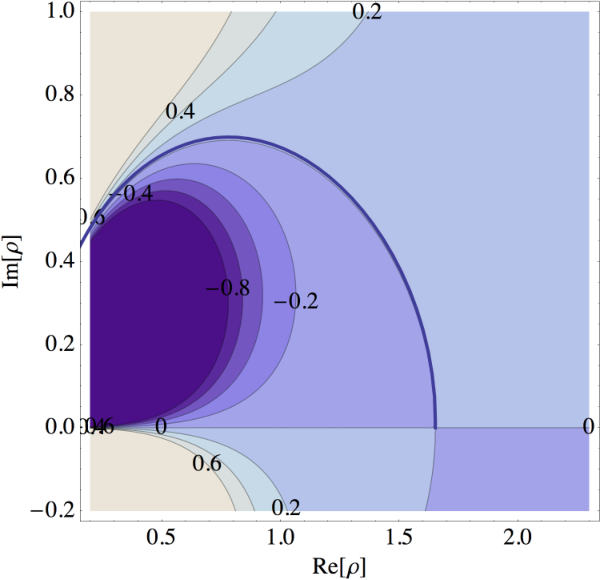
The computation of the one-point PDF relies on the following expression
| (106) |
where we explicitly denote the value of the density for which we want to compute the PDF. This is to distinguish it from the variable that enters in the calculation of out of the Legendre transform of . The idea to achieve fast convergence of the integral is to follow a path in the complex plane where the argument of the exponential in Eq. (106) is real. The starting point of the calculation is . When is small enough (in the regular region) then we simply have otherwise one should take . At this very location, 2 lines of vanishing imaginary part of cross, one along the real axis (obviously) and one parallel to the imaginary axis (precisely because we are at a saddle point position). The idea is then to build, step by step, a path by imposing
| (107) |
This condition can be written as an infinitesimal variation of . Recalling that , for each step we have to impose
| (108) |
which in turns can be obtained by imposing that the complex argument of is that of This is what we implement in practice. Accurate prediction for the PDFs are obtained with about 50 points along the path line.
B.2 The large density tails

The derivation of the rare event tail of the density PDF for large positive densities is based on the inverse Laplace transform of the generating function when it is dominated by its singular part, i.e. for . In this case the complex plane contour is pushed along the real axis wrapping around the singular value as depicted on Fig. 14.
The general form for the density PDF given by Eq. (106) is expressed using the form (41) following the path shown on Fig. 14. As the contributions from the two branches of the path lines are complex conjugate, it eventually leads to the form,
| (109) | |||||
where we keep only the dominant singular part in and where denotes the imaginary part. This integral can easily be computed and it leads to,
| (110) |
Subleading contributions can be computed in a similar way when is expanded to higher order. Note that by symmetry, only half integer terms that appear in this expansion will actually contribute.
Appendix C The constrained variance
In this appendix we complement the calculations started in Subsect. IV.5 where we computed the expected slope under a local density constraint. Pursuing along the same line of calculations, the variance of given can be computed from the conditional value of . It is given by the second derivative of the moment generating function, and is therefore given by
The calculation of its approximate form in the low- saddle point limit is a bit more cumbersome. Indeed, in the low variance limit in which this approximation is derived the two terms in the square brackets are not of the same order, the first being subdominant with respect the second. It is nonetheless possible to compute the resulting cumulant in the low density limit. Formally, differentiating Eq. (88) with respect to we have
| (111) |
from the Legendre stationary condition, which, after inversion of the partial derivatives, is formally given by
| (112) |
where are calculated at the stationary point. On the other hand can be expanded as
| (113) |
near the saddle point value . The integration of in the complex plane therefore leads to a correction from the term. It can be verified though that this contribution vanishes when one takes the cumulant. The integration of however leads to an extra term due to the second term in the previous expansion. The resulting term reads , so that
| (114) |
which can be rewritten more compactly as
| (115) |
when expressed in terms of .
Appendix D Simulations
For the purpose of this paper, we have carried out a dark matter simulation with Gadget2 [42]. This simulation is characterized by the following CDM cosmology: , , , kmMpc-1 and , within one standard deviation of WMAP7 results [43]. The box size is 500 Mpc sampled with particles, the softening length 24 kpc. Initial conditions are generated using mpgrafic [44]. The variances and running indexes are measured from the theoretical power spectra produced by mpgrafic. Snapshots are saved for and . An Octree is built for each snapshot, which allows us to count very efficiently all particles within a given sequence of concentric spheres of radii between up to . The center of these spheres is sampled regularly on a grid of aside, leading to 117649 estimates of the density per snapshot. All histograms drawn in this paper are derived from these samples. Note that the cells overlap for radii larger than .
Appendix E Systematic comparisons with simulation
We collect here figures that are too large to be put in the main text.