Anderson localization in two-dimensional graphene with short-range disorder: One-parameter scaling and finite-size effects
Abstract
We study Anderson localization in graphene with short-range disorder using the real-space Kubo-Greenwood method implemented on graphics processing units. Two models of short-range disorder, namely, the Anderson on-site disorder model and the vacancy defect model, are considered. For graphene with Anderson disorder, localization lengths of quasi-one-dimensional systems with various disorder strengths, edge symmetries, and boundary conditions are calculated using the real-space Kubo-Greenwood formalism, showing excellent agreement with independent transfer matrix calculations and superior computational efficiency. Using these data, we demonstrate the applicability of the one-parameter scaling theory of localization length and propose an analytical expression for the scaling function, which provides a reliable method of computing the two-dimensional localization length. This method is found to be consistent with another widely used method which relates the two-dimensional localization length to the elastic mean free path and the semiclassical conductivity. Abnormal behavior at the charge neutrality point is identified and interpreted to be caused by finite-size effects when the system width is comparable to or smaller than the elastic mean free path. We also demonstrate the finite-size effect when calculating the two-dimensional conductivity in the localized regime and show that a renormalization group beta function consistent with the one-parameter scaling theory can be extracted numerically. For graphene with vacancy disorder, we show that the proposed scaling function of localization length also applies. Lastly, we discuss some ambiguities in calculating the semiclassical conductivity around the charge neutrality point due to the presence of resonant states.
pacs
72.80.Vp, 72.15.Rn, 73.23.-b, 05.60.GgI Introduction
Graphene is an effectively two-dimensional (2D) material consisting of a sheet of carbon atoms. [1, 2] In its pristine form, it exhibits many remarkable low-energy electronic transport properties, such as half-integer quantum Hall effect [3, 4] and Klein tunneling, [5] due to the linear dispersion of the charge carriers near two inequivalent valleys around the charge neutrality point. However, disorder may dramatically alter both the electronic structure [6] and transport properties [7, 8, 9] of graphene. It is generally believed that both short-range [10, 11, 12, 13] and strong long-range [14] disorder can lead to inter-valley scattering and Anderson localization, while weak long-range disorder only gives rise to intra-valley scattering, which does not lead to backscattering and Anderson localization [15, 16, 17].
Due to its intrinsic low-dimensionality, graphene provides an ideal testbed of revisiting old ideas regarding Anderson localization in low dimensions as well as discovering new ones. The most successful theory for Anderson localization is one-parameter scaling [18], which predicts that all states in disordered one- and two-dimensional systems are localized at zero temperature if the system is sufficiently large, although exceptions can occur when the disorder is correlated [19] or electron-electron interaction cannot be neglected [20]. However, recent works regarding localization in graphene have yielded results that conflict with one-parameter scaling, with some studies supporting the existence of mobility edges even in the presence of uncorrelated Anderson disorder [21, 22]. Very recent numerical results indicate the difficulty of associating data for the finite-size localization length with a single scaling curve [23] as well as the discrepancy between results of the 2D localization length obtained from the finite-size scaling approach and the self-consistent theory of localization [24]. On the other hand, it has been suggested that the conductivity at the charge neutrality point (CNP) saturates to a constant value [25], or decays following a power-law rather than exponentially with increasing system size [26, 27], in graphene with resonant scatterers such as vacancy defects.
Since the typical length scales regarding localization properties in 2D systems are generally very large, efficient numerical methods are desirable. Although the standard numerical method for studying quantum transport is the Landauer-Büttiker approach combined with the recursive Green-function technique, using it for realistically sized truly 2D graphene systems is still beyond current computational ability, since the computational effort scales cubically with the width of the system. In contrast, the linear-scaling real-space Kubo-Greenwood (RSKG) method [28, 29, 30, 31] is generally much more efficient and has been used to study electronic transport in realistically sized graphene with various kinds of disorder [26, 27, 32, 33, 34, 35, 36]. In this method, the actual computational effort depends on the energy resolution, the required statistical accuracy, and most crucially, the transport regime. Exploring the localization properties generally requires a large simulation cell to eliminate possible finite-size effects and a long correlation time (which can be thought as the evolution time of a wavepacket) to actually reach the localized regime, which can be very time-consuming. Recently, we have significantly accelerated the calculations by implementing [37] this method on graphics processing units [38], and further developed methods for obtaining the localization properties of disordered systems. It has been established [39] through comparisons with the standard Landauer-Büttiker approach that (1) the average propagating length of electrons can serve as a good definition of length before its saturation and (2) the saturated propagating length is directly proportional to the localization length defined in terms of the exponential decay of conductance in the strongly localized regime.
Armed with this efficient numerical method, we perform an extensive numerical study of Anderson localization in graphene with short-range disorder, including Anderson disorder and vacancies. We first calculate the localization lengths for various quasi-one-dimensional (Q1D) systems using the RSKG method. Since most of the previous works [12, 23, 24, 40] have applied the transfer matrix method (TMM) [41] (or equivalently, the recursive Green-function method, see Ref. 42), we also present a comparison between these two methods. Based on our computational data, we are able to compare the results against the one-parameter scaling theory of localization length [42, 43] and construct an analytical expression for the so far undetermined scaling function. Our results are consistent with those of Schreiber and Ottomeier [40] and Lee et al. [24], but compared to these works, we have considered a more complete set of energy points and much wider systems. We will also discuss the finite-size effects for the scaling analyses of both localization length and conductivity and some ambiguities in determining the semiclassical conductivity in graphene with resonant disorder using the RSKG method.
This paper is organized as follows. Section II defines the physical models and introduces the TMM for the calculation of localization length and the RSKG method for the calculation of localization length as well as other electronic and transport properties. We then study Anderson localization of graphene with Anderson disorder and vacancy-type disorder in Sections III and IV, respectively. Section V concludes.
II models and methods
II.1 Models
For pristine graphene, we apply the widely used nearest-neighbor orbital tight-binding Hamiltonian
| (1) |
where is the hopping parameter. The uncorrelated Anderson disorder is modeled by adding random on-site potentials uniformly distributed within an energy interval of , being a measure of the disorder strength. The more realistic vacancy disorder is modeled by randomly removing carbon atoms according to a prescribed defect concentration , which is defined to be the number of vacancies divided by the number of carbon atoms in the pristine system. We will consider the whole energy spectrum for the Anderson model and thus take as the unit of energy, but only consider a small energy window for the vacancy model and take eV as the unit of energy and set eV. When calculating the Q1D localization length, we will consider both zigzag and armchair graphene nanoribbons (ZGNRs and AGNRs, correspondingly). To test the effect of the boundary conditions in the transverse direction, we also consider armchair carbon nanotubes (ACNTs) with the transport direction along the zigzag edge and periodic boundary conditions also along the transverse direction. We use and to denote the number of dimer lines along the zigzag edge and the number of zigzag-shaped chains across the armchair edge, respectively. The total number of carbon atoms in the computational cell is then . The symbol defines the width of the system. For ZGNRs and ACNTs, we set to and obtain the actual width using . For AGNRs, we set to and obtain the actual width using . Here, is the carbon-carbon distance, being roughly 0.142 nm.
II.2 Methods
We define the localization length of a Q1D system with a fixed width to be the characteristic length of the exponential decay of typical conductance with the system length in the strongly localized regime [44]:
| (2) |
where the typical conductance is obtained from the ensemble average over individual realizations with fixed system size and disorder strength [45].
In the literature, the most often used methods for computing are the recursive Green-function method and the TMM, which are essentially equivalent [42]. In Ref. 39, we have suggested another method of finding using the RSKG formalism, briefly explained below. In this work, we will further demonstrate its accuracy and efficiency by comparing it against the TMM.
II.2.1 The transfer matrix method
In the TMM, the wave function of the th slice along the transport direction of the Q1D geometry is calculated iteratively using the transfer matrix equation (note that all the matrix or vector elements here are -by- matrices) as
| (3) |
with the initial wave functions and . We only consider ZGNRs and ACNTs (both with the transport direction along the zigzag edge) when using the TMM, where the matrix takes two alternative forms depending on whether is even or odd, as given in Ref. 40. According to Oseledec’s theorem [46], with increasing , the eigenvalues of , where , converge to fixed values , the being Lyapunov exponents. The localization length is defined as the largest decaying length associated with the minimum Lyapunov exponent [44]:
| (4) |
Numerically, the minimum Lyapunov exponent can be computed by combining Gram-Schmidt orthonormalization with the above transfer matrix multiplication. Practically, only sparse matrix-vector multiplication is required and one does not need to perform Gram-Schmidt orthonormalization after each multiplication. Usually, performing one Gram-Schmidt orthonormalization every ten multiplications keeps a good balance between speed and accuracy. The number of slices required for achieving a relative accuracy of is approximately [42] . In this work, we set .
II.2.2 The real-space Kubo-Greenwood method
In the RSKG method [28, 29, 30, 31], the zero-temperature dc electrical conductivity at energy and correlation time can be expressed as
| (5) |
where
| (6) |
is the electronic density of states with the spin degeneracy taken into account. Note that the factors of 2 in the above two equations can cancel each other and are not presented in some works, but we prefer to keep them for clarity. Here, is the Hamiltonian and is the volume, or in our case, just the area of the graphene sheet, and
| (7) |
is the mean square displacement. is the position operator and is the time-evolution operator. What need to be calculated are and at a chosen set of . The so-called linear-scaling algorithm for calculating the latter (the calculation of the former does not need the second technique below) can be achieved by the following three techniques: (1) approximating the trace by using one or a few random vectors , , being an arbitrary operator, (2) calculating the time-evolution of iteratively using, e.g., the Chebyshev polynomial expansion, and (3) approximating the Dirac delta function using a linear-scaling technique such as Fourier transform, Lanczos recursion, or kernel polynomial. The relative error caused by the random-vector approximation is proportional to [47] , where is the Hamiltonian size (the total number of carbon atoms in our problems) and is the number of independent random vectors used. In this work, we have used a few to a few tens of random vectors for each simulated system, the specific number depending on the specific system, the required accuracy, and the specific quantities to be calculated. For the approximation of the Dirac delta function, we have used the kernel polynomial method [47]. The energy resolution achieved using this method is inversely proportional to the number of Chebyshev moments (which is the order the Chebyshev polynomial expansion) used. For most of the calculations, we have chosen to be 3000, which corresponds to en energy resolution of a few meV. While this energy resolution is sufficiently high for graphene with Anderson disorder, it is not neccesarily high enough to distinguish the resonant state at the CNP in graphene with vacancy defects from other states. In Section IV.4, we will disscuss the effect of energy resolution on the results for graphene with vacancy defects. Details of the involved algorithms and the implementation on graphics processing units can be found in Ref. [37].
As increases from zero, the running conductivity first increases linearly, indicting a ballistic behavior, and then gradually saturates to a fixed value, which can be interpreted as the semiclassical conductivity , and finally decreases until it becomes zero if localization takes place. In practice, especially when the disorder is strong, there may be no apparent plateau to which the running conductivity saturates, and is thus usually defined as the maximum of . While this is generally a reasonable definition, it can sometimes result in problems, as we will show in Section IV.3. After obtaining , one can calculate the elastic mean free path through the Einstein relation for diffusive transport [48]:
| (8) |
where is the Fermi velocity, which can be calculated from the velocity auto-correlation at zero correlation time [37].
The usefulness of the RSKG method also depends crucially on a definition of propagating length in terms of . Indeed, in the original Kubo-Greenwood formalism, there is no definition of length and no connection between conductivity and conductance can be made. A definition of length is required for the study of mesoscopic transport properties. A natural definition would be , but a more precise relation has been established [37, 39]:
| (9) |
The factor of 2 in this equation can be justified from different perspectives: (1) it results in [37] the textbook formula [49] for the ballistic conductance
| (10) |
and (2) it results in a Q1D conductance which is consistent with independent Landauer-Büttiker calculations in the localized regime [39]. This definition of length is only valid up to about , after which the propagating length saturates to a fixed value proportional to the localization length [39, 44]:
| (11) |
The meaning of the factor of in this equation is yet to be found, but this expression yields results in a good agreement with independent Laudauer-Büttiker calculations [39]. Although an infinite is indicated in the above equation, in practice, we only simulate up to a finite and then fit the mean square displacement data using a Padé approximant of the form . We found that as long as the mean square displacement is almost converged, this simple Padé approximant results in a very good fit to the data and the saturated mean square displacement can be extracted as . As in the case of the TMM, an error estimation of the calculated data is useful to evaluate the quality of the results. However, there seems to be no unique way to define the errors for calculated using the RSKG method. We have estimated the error for as the mean of over , where is the fitted propagating length using the Padé approximant. We will further validate this method by comparing with independent TMM calculations in Section III.1 and discuss the finite-size effect in this method caused by the finite simulation cell length in Section IV.1.
III Graphene with Anderson disorder
III.1 Localization lengths for quasi-one-dimensional systems


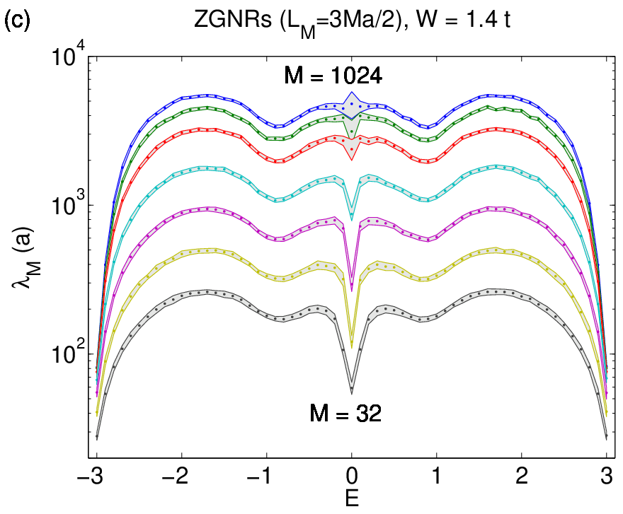

Figure 1 shows the calculated localization lengths for Q1D systems with different widths, energies, disorder strengths, edge types, and boundary conditions. The considered systems are (a) ZGNRs with , (b) ACNTs with , (c) ZGNRs with , and (d) AGNRs with . In Figs. 1(a) and 1(b), the open circles and small filled dots correspond to the results obtained by the TMM and the RSKG method, respectively. The errors estimates for the RSKG results are indicated by the shaded areas with bounding lines. The relative accuracy of the TMM results is set to , which would result in errors comparable to the corresponding marker size, and we thus omit the error bars for the TMM results for simplicity. Both methods give practically the same results, but the RSKG method is much more efficient for wider systems due to the use of linear scaling techniques and the intrinsic parallelism in energy of this method. The parallelism in energy means that obtaining the results for all the energy points does not require more computation time than obtaining the result for a single energy value. In contrast, the computation time for the TMM scales cubically with respect to the width of the system and there is no parallelism in energy. Therefore, using the TMM, we have only calculated a limited number of energy points for and 256 and no points for . Even under these conditions, the computation times for these two methods are roughly equal, which demonstrates the accuracy and efficiency of the RSKG method. We thus only used the RSKG method for weaker disorder, as shown in Figs. 1(c) and 1(d).
There is an obvious difference between the results for different boundary conditions and edge types. Figures 1(a) and 1(b) correspond to transport in the direction of the zigzag edge, and differ only by the boundary conditions used in the transverse direction, with Fig. 1(a) corresponding to free (hard wall) boundary conditions (ZGNRs) and Fig. 1(b) to periodic boundary conditions (ACNTs). We note that for ACNTs, the CNP behaves rather differently from the other points: it evolves from a local maximum for to a local minimum for . This observation is consistent with the finding by Xiong et al. [12]. Figures 1(c) and 1(d) correspond to a weaker disorder with , with Fig. 1(c) showing results for ZGNRs and 1(d) for AGNRs. To avoid band gaps, only metallic AGNRs are considered. We note that AGNRs behave similarly as ACNTs, having a maximum of at the CNP when the width of the system is small. However, with increasing width, the differences between different boundary conditions and edge types become smaller, and one may expect that these differences become vanishingly small in the limit of wide systems.
III.2 One-parameter scaling of localization length

As our results indicate that the differences of localization lengths between different boundary conditions and edge types become smaller with increasing width, a natural question is whether the conventional one-parameter scaling theory of localization length applies to our simulation data. MacKinnon and Kramer [42, 43] have proposed the following scaling law for the Q1D localization length:
| (12) |
where is the 2D localization length for a given and , and is an unknown function. The construction of the scaling function for graphene (or honeycomb lattice) has been considered by Schreiber and Ottomeier [40] as early as in 1992, although they only considered relatively strong disorder () due to the limited computational power available at that time. Recently, Lee et al. [24] constructed a scaling curve for systems with down to , although not all the energy points (especially some points at and around the CNP) were considered uniformly. An inspection of the scaling curves presented in Refs. [40] and [24] reveals that the scaling function may be universal. Thus, it is natural to attempt to construct an analytical expression for this scaling function.
To find such a universal function, we note that when is in the Q1D limit, where (i.e., ) (but should be large enough to ensure that enters the scaling regime), decays nearly linearly with increasing (not shown here). This indicates that , where and are constants. This kind of asymptotic behavior was in fact noticed very early by MacKinnon and Kramer [42]. On the other hand, they also noted that when (i.e., ), and the scaling function should behave as . A natural choice for the scaling function which meets these two conditions simultaneously is thus , or equivalently,
| (13) |
where is a constant which needs to be determined numerically. Before testing this function against our data, we point out that finding a parametrized analytical expression for the scaling function is not in sharp contrast with previous works. On the one hand, it is conventional to assume an analytical form for the scaling function when studying Anderson localization in three-dimensional systems [50, 51], and following this approach, different functions have been tested for simulation data for graphene flakes [23]. On the other hand, it has been assumed that in the limit of the scaling function takes the following parametrized form [24, 42]:
| (14) |
where is a fitting parameter. It is clear that Eq. (13) automatically results in this kind of asymptotic behavior when .
We have fitted the data of Fig. 1 against Eq. (13), treating the 2D localization lengths for every and as independent fitting parameters. The results are shown in Fig. 2. We have only used the data for the three systems having the largest localization lengths in each of the Figs. 1(a)-(d)), since data for relatively narrow systems apparently do not follow any scaling curve. Nevertheless, our data already spread over a broader range of system widths compared to previous works [40, 24]. Accidentally or not, we estimate that the value of the parameter in Eq. (13) is very close to . As can be seen from Fig. 2, all the data points project well onto the scaling curve, except for the CNP in the two weakly disordered () systems. The reason why the CNP experiences the largest finite-size effect will be discussed later. The scaling function, Eq. (13) with , also gives an excellent description for the data in Ref. [24] [52], as well as for the data for k square lattice with uncorrelated Anderson disorder, as shown in Appendix A, and for the data for graphene with vacancy-type disorder, as will be discussed in Section IV.3. While the simulation data agree well with the proposed scaling function, in the next subsection we will further explore its connection to another widely used method of computing the 2D localization length.
III.3 Comparing two methods of computing the 2D localization length


According to the scaling theory of Anderson localization [53, 54, 55, 56], can also be estimated exclusively based on the diffusive transport properties [44]:
| (15) |
It is thus important to ask whether this expression is consistent with the scaling approach based on the Q1D localization length. To answer this question, we first calculate the diffusive transport properties for systems with and . The results are shown in Fig. 3. Note that the results are not sensitive to the edge type or boundary conditions, since the relevant transport length scale, the mean free path , is relatively small (compared to ), and we can use a sufficiently large simulation cell size to eliminate any finite-size effects affecting the diffusive transport properties. An examination of Fig. 3 reveals why the CNP behaves very differently from other states regarding the localization properties. At the CNP, the density of states is vanishingly small but the semiclassical conductivity and the group velocity are of the same order as for other states. This results in a very large at the CNP, as has also been found by Lherbier et al. [32]. With a disorder strength of , at the CNP, which is comparable to the simulation widths used for calculating the Q1D localization lengths. One cannot expect that the scaling function applies when , because sets up a lower limit of the scaling behavior [42]. More quantitatively, should be at least several times larger than to make the scaling function fully applicable. However, with decreasing disorder strength, for the CNP diverges and it becomes formidable to reach the scaling regime computationally.
Figure 4 compares the localization lengths calculated by Eq. (13) (with ) and Eq. (15). We can see that the 2D localization lengths are much larger than the Q1D values, making a direct computation nearly impossible. They also depend sensitively on the disorder strength, with the values for being several orders of magnitude larger than those for . With a given disorder strength, the values of obtained using Eq. (13) with different boundary conditions and edge types are very close to each other, only exhibiting some discrepancies around the CNP, which, as have been noted before, should be originated from the finite-size effect. It can be seen that the two methods for computing agree well with each other. Lee et al. [24] also compared these two methods, but in contrast to our results, observed that Eq. (15) results in a significant underestimation. Our interpretation is that their method of computing is based on the semiclassical self-consistent Born approximation, which may be not as accurate as the fully quantum mechanical RSKG method.
The fact that Eq. (13) and Eq. (15) give consistent results for can be understood in the following way. We know that in the Q1D limit, the localization length and the mean free path are related by the Thouless relation [57, 58, 59, 60] (for the orthogonal universality class, which is the case for graphene with intervalley scattering) [44]:
| (16) |
where is the number of transport channels. In other words, equals the “hypothetical” ballistic conductance as given by Eq. (10) divided by the conductance quantum :
| (17) |
By “hypothetical”, we mean that is the conductance of the disordered system in the zero length limit, where no scattering starts to play a role. By combining the above two equations and using the relation between and in Eq. (8), we arrive at the following modified version of the Thouless relation:
| (18) |
In the Q1D limit, the scaling function given by Eq. (13) (with ) can be written as , which, combined with the above Thouless relation, gives
| (19) |
Choosing gives exactly Eq. (15). This heuristic derivation is consistent with the intuition that the scaling regime starts from a width several times larger than the mean free path.
III.4 One-parameter scaling of conductivity


The one-parameter scaling of localization length is in fact intimately connected [42] to the one-parameter scaling of conductivity. Equation (15) has been derived from the scaling behavior of the 2D conductivity in the weak localization regime, where the conductivity decays logarithmically with increasing :
| (20) |
Here is a length scale, conventionally set to . Assuming that reaches when the weak localization correction becomes comparable to gives Eq. (15) apart from a factor of 2 resulting from the use of different conventions [44].
The validity of the weak localization formula, Eq. (20), can also be confirmed numerically. Figure 5(a) shows the calculated conductivity as a function of the propagating length, as defined by Eq. (9), for the state with and . The calculated conductivities are ensemble averaged over several disorder realizations and the tracing operation in Eq. (7) has been approximated using several random vectors, resulting in relatively smooth curves. Due to the large localization length in 2D, significant finite-size effects arise when calculating the conductivity in the localized regime. When the simulation size increases from to , the calculated data get closer to the line predicted by Eq. (20), with being set to the “diffusion length” (which is generally larger than the mean free path) beyond which the conductivity starts to decay. is defined as the length at which the running conductivity reaches its maximum value [33, 34]. Although periodic boundary conditions are applied in both the transport and the transverse directions, we see that a simulation size of is not large enough to eliminate the finite-size effect, resulting in an artificial fast decay of conductivity when .
The transition from the weak to the strong localization regime is smooth and universal. Figure 5(b) shows the conductivity as a function of the propagating length normalized by the 2D localization length. The data for different energy states project onto a single curve, which agrees with the scaling theory of localization. This indicates the existence of a universal renormalization group function:
| (21) |
as shown in the inset of Fig. 5(b). The scaling function behaves as when , which is consistent with the exponential decay of conductivity in the strongly localized regime. Similar results have been obtained [61] for hydrogenated graphene using the Landauer-Büttiker approach. One may note that different renormalization group functions, either with [15] or without [16] an unstable fixed point, have been obtained for graphene with long-range disorder. While the positive sign of the functions (in the large conductivity limit) in the previous works signifies antilocalization in the absence of intervalley scattering, the negative sign of the function in our work is associated with localization caused by intervalley scattering.
IV Graphene with vacancy disorder
Although the Anderson disorder model is of general theoretical interest, more realistic short-range scatterers in graphene are atomically sharp defects, such as vacancies and adatoms, which are believed to cause intervalley scattering and Anderson localization around the CNP in irradiated graphene[62] and hydrogenated graphene [63]. Here, we focus on the vacancy-type disorder, which also approximates the effect of hydrogen adatoms [64].
IV.1 Finite-size effect resulting from the finiteness of the simulation length

Before presenting the results for graphene with vacancy defects, we first discuss the finite-size effect for the calculation of the Q1D localization length using the RSKG method. This finite-size effect is different from that which causes the deviations of the data for the CNP from the scaling function in Fig. 2. It is a finite-size effect caused by the use of a finite simulation length in practical calculations. In the RSKG method, the propagating length , defined by Eq. (9), serves as a measure of the actual length of the physical system at a specific correlation time. In contrast, the simulation cell length, which is proportional to (or , depending on the transport direction) has no direct connection to . Usually, periodic boundary conditions are applied along the transport direction to alleviate the finite-size effect caused by the finiteness of . Whether or not a given is large enough to eliminate the finite-size effect depends on the involved transport length scales. Figure 6 shows the finite-size effect when calculating the Q1D localization lengths for ACNTs of width with vacancies. As the simulation cell length increases from to , the calculated Q1D localization lengths converge, which reflects the alleviation of the finite-size effect by increasing the simulation cell length. It is clear to see that states with larger saturated localization lengths require larger simulation cell lengths to eliminate the finite-size effect. More quantitatively, to completely eliminate the finite-size effect, the simulation cell length should be a few times larger than the maximum localization length for a given simulated system. In this paper, we have used as large as possible simulation cell lengths, and the finite-size effects resulting from the finiteness of have been practically eliminated.
IV.2 One-parameter scaling of localization length

We have calculated the localization lengths for Q1D graphene systems in the ACNT geometry with , 256, and 512, with the vacancy concentration fixed to . The results are shown in the inset of Fig. 7. The main frame of Fig. 7 shows that the scaling function given by Eq. (13), with , also applies here. A striking difference between vacancy disorder and Anderson disorder is that the Van Hove singularities at are much more strongly affected by Anderson disorder (manifested in the local minimum of the mean free path at in Fig. 3), while vacancies mostly affect low-energy charge carriers around the CNP. This is because vacancies serve as high potential barriers which result in large scattering cross sections and small mean free paths for low-energy charge carriers [60]. In contrast, high-energy charge carriers experience small scattering cross sections and have large mean free paths, which combined with higher densities of states (larger number of transport channels), gives rise to large Q1D localization lengths according to the Thouless relation. For the selected defect concentration, our numerical calculations are only able to explore a small energy range eV around the CNP. Within this energy range, all the data agree well with Eq. (13), and the corresponding 2D localization length can thus be extracted.
IV.3 Connecting diffusive and localized transport regimes


As in the case of graphene with Anderson disorder, one may ask whether the 2D localization lengths obtained by fitting the Q1D data against Eq. (13) are consistent with those obtained by using Eq. (15). It turns out that there is some ambiguity in the calculation of the semiclassical conductivity at the CNP, as shown in Fig. 8(a), where the running conductivity obtained by using Eq. (5) is compared with that obtained by substituting the time derivative in Eq. (5) with a time division. The latter may be well described by a power-law length-dependence in an appropriate regime [26, 27], and is thus associated with an infinite localization length, as suggested in the previous works. However, the correct derivative-based definition of does not support the power-law length dependence. The calculated develops more than one peak, which may just reflect the radial distribution profile of the local density of states, which has large magnitude in the vicinity of the vacancies [65]. In the RSKG method, as the wavepackets (associated with individual sites) propagate, they can “feel” a large local density of states associated with the conductivity peak before reaching the diffusive regime. Unfortunately, there does not seem to be any completely unambiguous method in the RSKG formalism for determining a diffusive regime where a well defined value of can be extracted. When moving away from the CNP, the effect of the local density of states diminishes, and there is no such local peaks of conductivity, as shown by the results for eV in Fig. 8(a).
The large local density of states at the CNP affects the conductivity significantly only in the ballistic-to-diffusive regime. In the strongly localized regime, we expect that the conductivity decays exponentially with increasing length. This is confirmed by the results shown in Fig. 8(b). Here, the simulation data can be well described by the exponential fitting[44]: . Even the conductivity at the CNP obtained by approximating the time-derivative with a time-division follows the exponential law in the strongly localized regime, although this approximation results in a much larger value of conductivity at a given length.
Figure 9 shows the 2D localization lengths calculated by Eq. (15) and Eq. (13), along with those for and 0.1 eV extracted using the exponential fitting. Here, the semiclassical conductivity is taken to be the maximum of the running conductivity when applying Eq. (15). The agreement between Eq. (15) and Eq. (13) is good only at higher energies. At the CNP, the prediction of Eq. (15) is far too large compared to that given by Eq. (13). In contrast, the exponential fitting gives rise to results consistent with Eq. (13). We thus conclude that the discrepancy between Eq. (15) and Eq. (13) is largely resulted from the ambiguity in the calculation of the semiclassical conductivity.
IV.4 Effects of energy resolution and vacancy concentration
Due to the large density of states around the CNP, one may expect that the energy resolution used in the numerical calculations would affect the results. To see how the energy resolution affects the results, we first calculate the density of states and running conductivity for graphene with vacancy defects using different values of , the number of Chebyshev moments in the kernel polynomial method. Although there may be no exact relationship between and , it is generally believed [47] that . Therefore, one can increase the energy resolution, i.e., decrease , by increasing .
Figure 10 presents the results for the density of states and the maximum conductivity (over the correlation time), the latter being conventionally taken as the definition of in the RSKG method. It can be seen that with increasing energy resolution, both and develop increasingly high values at the CNP. In contrast, the results for the other energy points do not depend on the energy resolution. Interestingly, is proportional to , as shown in Fig. 10(c). Then, one may ask if the length-dependence of the conductivity at the CNP also depends crucially on the energy resolution. To answer this question, we have plotted the running conductivity as a function of the propagating length at the CNP, obtained by using different energy resolutions, in Fig. 11(a). It can be seen that when , i.e., roughly in the ballistic-to-diffusive regime, the results depend strongly on the energy resolution. Outside this regime, the dependence disappears with increasing , with the results being converged when . Moreover, it can be seen that the energy resolution does not affect the obtained localization length. Figure 11(b) shows the running conductivity at eV, also obtained using different energy resolutions. The energy resolution does not seem to significantly affect the results at any length scale away from the CNP.
So far, we have only considered a relatively large vacancy concentration of . We now study how the defect concentration affects the scaling of conductivity at the CNP, by additionally considering systems with lower vacancy concentrations: and . The results are shown in Fig. 12. In the main frame, we have plotted the running conductivity as a function of the normalized propagating length , where is the average distance between an atom and its nearest vacancy. From simple geometric considerations, one can find that
| (22) |
which can also be confirmed by numerical calculations. One can make several observations based on Fig. 12:
(1) The maximum values of the running conductivity are different for different vacancy concentrations ; a higher gives a higher . This indicates that the peak of the running conductivity is related to the local density of states around the vacancies.
(2) For all the considered vacancy concentrations, the running conductivity takes its maximum at ( in Fig. 12). This further supports our suggestion that the peak of the running conductivity is directly related to the local density of states around the vacancies, since is also the distance at which the radial distribution function of the local density of states attains its peak value.
(3) Beyond the ballistic-to-diffusive regime, i.e., when , the running conductivities for different vacancy concentrations are well correlated and decay exponentially with increasing length. This is strong evidence for the validity of the one-parameter scaling. Since , the running conductivities are also correlated when plotted as a function of , as shown in the inset of Fig. 12. Our results are qualitatively different from those by Ostrovsky et al. [25]. Using a different numerical method, they found that the running conductivity saturates to a constant on the order of with increasing , without localization even up to . We are not sure about the origin of the different results, but we note that Ostrovsky et al. have remarked that [25] the systems will eventually enter the localized regime with increasing vacancy concentration.
(4) Based on the correlation in the main frame of Fig. 12, we can infer that the localization length is proportional to , which is in turn proportional to the average distance between the vacancies. Based on the analysis of the effective cross sections [60], we know that the mean free path is also proportional to . Therefore, the (2D) localization length at the CNP is directly proportional to the mean free path, indicating [according to Eq. (15)] that at the CNP does not depend on the vacancy concentration. Taking the mean free path as , we estimate that at the CNP. Using this value for , the discrepancy between Eq. (15) and Eq. (13) at the CNP disappears.


Although the CNP has a very large density of states coming from the resonant states (mid-gap states), it is the most localized state, exhibiting the smallest localization length. The state at the CNP is a quasilocalized state [65] and also exhibits a peak value of the inverse participation ratio [66]. Therefore, Anderson localization can be observed around the CNP, manifesting itself as conductivities smaller than the minimum conductivity of pristine graphene. However, when moving away from the CNP, the localization length increases quickly, even up to values much larger than realistic sample sizes or coherence lengths. For a fixed sample size, the localization effect is only significant around the CNP and disappears rapidly with increasing energy (or carrier concentration), which may result in an effective mobility edge and metal-insulator transition.
V Conclusions
In summary, we have presented a systematical numerical study of Anderson localization in graphene with short-range disorder, using the real-space Kubo-Greenwood formalism and simulating uncorrelated Anderson disorder and vacancy defects. For graphene with Anderson disorder, the localization lengths for various quasi-one-dimensional systems with different widths , disorder strengths, energies, edge types, and boundary conditions were calculated, and results for smaller systems were checked against the standard transfer matrix method with good agreement. We have found that the localization lengths can be well described by a simple scaling function, , with being close or equal to . Deviations from this scaling law occur due to finite-size effects, which manifest themselves when is comparable to or even smaller than the mean free path . The two-dimensional localization lengths obtained using this scaling function are found to be consistent with the approximation based on diffusive transport properties: , where is the semiclassical conductivity and is the conductance quantum. By calculating the 2D conductivity in the weak and strong localized regimes, with the finite-size effects identified and eliminated by using sufficiently large simulation domain size, we also obtained a universal renormalization group function for 2D conductivity. For graphene with vacancy disorder, we have demonstrated another finite-size effect in the real-space Kubo-Greenwood method, which occurs when the simulation cell length is not sufficiently large compared with . Surprisingly, the same scaling function proposed based on the results for Anderson disorder also applies to graphene with vacancy defects. The charge neutrality point in graphene with vacancy defects, however, exhibits an abnormally large peak value for the running conductivity in the ballistic-to-diffusive regime. We have suggested that this abnormal behavior may be resulted form the local density of states caused by the resonant states located around the vacancy sites and presented evidence that the charge neutrality point is exponentially localized. Our work thus suggests that the localization behavior of graphene with short-range disorder is to a large extent similar to conventional two-dimensional systems (such as the square lattice studied in the Appendix).
Acknowledgements.
We thank A.-P. Jauho, K. L. Lee, D. Mayou, R. Mazzarello, S. Roche, R. A. Römer, T.-M. Shih, and I. Zozoulenko for helpful discussions and comments. This research has been supported by the Academy of Finland through its Centres of Excellence Program (Project No. 251748). We acknowledge the computational resources provided by Aalto Science-IT project and Finland’s IT Center for Science (CSC).Appendix A Square lattice with Anderson disorder
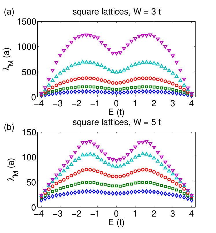
In this appendix, we show that the scaling function in Eq. (13) with also applies to a square lattice with uncorrelated Anderson disorder, i.e., random on-site potentials uniformly distributed in an interval of . To this end, we first calculate the Q1D localization lengths using Eq. (11). Figures 13(a) and 13(b) show the results for and , respectively. As can be seen from Fig. 14, all the data with are correlated by the scaling function very well, without any abnormal behavior resulting from the finite-size effect. Even the maximum mean free path for the square lattice with the weaker disorder strength, , is less than , which is well below the smallest value of considered. Therefore, all the data are in the scaling regime and follow the scaling curve. The obtained 2D localization lengths are shown in the inset, from which we see that the results for the band center are consistent with previous results by Schreiber and Ottomeier [40]. The results for other points away from the band center with are also consistent with those by Zdetsis et al. [67], exhibiting maximum values of around .

References
- [1] A. K. Geim and K. S. Novoselov, Nat. Mater. 6, 183 (2007).
- [2] M. I. Katsnelson, Graphene: Carbon in Two Dimensions (Cambridge University Press, Cambridge, England, 2012).
- [3] K. S. Novoselov, A. K. Geim, S. V. Morozov, D. Jiang, M. I. Katsnelson, I. V. Grigorieva, S. V. Dubonos, and A. A. Firsov, Nature, 438, 197 (2005).
- [4] Y. Zhang, Y.-W. Tan, H. L. Stormer, and P. Kim, Nature, 438, 201 (2005).
- [5] M. I. Katsnelson, K. S. Novoselov, and A. K. Geim, Nat. Phys. 2, 620 (2006).
- [6] A. H. Castro Neto, F. Guinea, N. M. R. Peres, K. S. Novoselov, and A. K. Geim, Rev. Mod. Phys. 81, 109 (2009).
- [7] N. M. R. Peres, Rev. Mod. Phys. 82, 2673 (2010).
- [8] E. R. Mucciolo and C. H. Lewenkopf, J. Phys.: Condens. Matter, 22, 273201 (2010).
- [9] S. Das Sarma, S. Adam, E. H. Hwang, and E. Rossi, Rev. Mod. Phys. 83, 407 (2011).
- [10] I. L. Aleiner and K. B. Efetov, Phys. Rev. Lett. 97, 236801 (2006).
- [11] A. Altland, Phys. Rev. Lett. 97, 236802 (2006).
- [12] S.-J. Xiong and Y. Xiong, Phys. Rev. B 76, 214204 (2007).
- [13] G. Schubert, J. Schleede, K. Byczuk, H. Fehske, and D. Vollhardt, Phys. Rev. B 81, 155106 (2010).
- [14] Y.-Y. Zhang, J. Hu, B. A. Bernevig, X. R. Wang, X. C. Xie, and W. M. Liu, Phys. Rev. Lett. 102, 106401 (2009).
- [15] P. M. Ostrovsky, I. V. Gornyi, and A. D. Mirlin, Phys. Rev. Lett. 98, 256801 (2007).
- [16] J. H. Bardarson, J. Tworzydlo, P. W. Brouwer, and C. W. J. Beenakker, Phys. Rev. Lett. 99, 106801 (2007).
- [17] K. Nomura, M. Koshino, and S. Ryu, Phys. Rev. Lett. 99, 146806 (2007).
- [18] E. Abrahams, P. W. Anderson, D. C. Licciardello, and T. V. Ramakrishnan, Phys. Rev. Lett. 42, 673 (1979).
- [19] A. Rodriguez, A. Chakrabarti, and R. A. Römer, Phys. Rev. B 86, 085119 (2012).
- [20] A. Punnoose and A. M. Finkel’stein, Science 310, 289 (2005).
- [21] M. Amini, S. A. Jafari, and F. Shahbazi, Europhys. Lett. 87, 37002 (2009).
- [22] Y. Song, H. Song, and S. Feng, J. Phys.: Condens. Matter. 23, 205501 (2011).
- [23] C. González-Santander, F. Domínguez-Adame, M. Hilke and R. A. Römer, Europhys. Lett. 104, 17012 (2013).
- [24] K. L. Lee, B. Gremaud, C. Miniatura, and D. Delande, Phys. Rev. B 87, 144202 (2013).
- [25] P. M. Ostrovsky, M. Titov, S. Bera, I. V. Gornyi, and A. D. Mirlin, Phys. Rev. Lett. 105, 266803 (2010).
- [26] A. Cresti, F. Ortmann, T. Louvet, D. Van Tuan, and S. Roche, Phys. Rev. Lett. 110, 196601 (2013).
- [27] G. T. de Laissardière and D. Mayou, Phys. Rev. Lett. 111, 146601 (2013).
- [28] D. Mayou, Europhys. Lett. 6, 549 (1988).
- [29] D. Mayou and S. N. Khanna, J. Phys. I Paris 5, 1199 (1995).
- [30] S. Roche and D. Mayou, Phys. Rev. Lett. 79, 2518 (1997).
- [31] F. Triozon, J. Vidal, R. Mosseri, and D. Mayou, Phys. Rev. B 65, 220202(R) (2002).
- [32] A. Lherbier, B. Biel, Y.-M. Niquet, and S. Roche, Phys. Rev. Lett. 100, 036803 (2008).
- [33] N. Leconte, A. Lherbier, F. Varchon, P. Ordejon, S. Roche, and J.-C. Charlier, Phys. Rev. B 84, 235420 (2011).
- [34] A. Lherbier, S. M.-M. Dubois, X. Declerck, Y.-M. Niquet, S. Roche, and J.-C. Charlier, Phys. Rev. B 86, 075402 (2012).
- [35] T. M. Radchenko, A. A. Shylau, and I. V. Zozoulenko, Phys. Rev. B 86, 035418 (2012).
- [36] A. R. Botello-Méndezn, A. Lherbier, and J.-C. Charlier, Solid State Commun. 175-176, 90 (2013).
- [37] Z. Fan, A. Uppstu, T. Siro, and A. Harju, Comput. Phys. Commun. 185, 28 (2014).
- [38] A. Harju, T. Siro, F. Canova, S. Hakala, and T. Rantalaiho, Lecture Notes in Computer Science 7782, 3 (2013).
- [39] A. Uppstu, Z. Fan, and A. Harju, Phys. Rev. B 89, 075420 (2014).
- [40] M. Schreiber and M. Ottomeier, J. Phys.: Condens. Matter. 4, 1959 (1992).
- [41] J. L. Pichard and G. Sarma, J. Phys. C: Solid State Phys. 14, L617 (1981).
- [42] A. MacKinnon and B. Kramer, Z. Phys. B 53, 1 (1983).
- [43] A. MacKinnon and B. Kramer, Phys. Rev. Lett. 47, 1546 (1981).
- [44] Note that there are different conventions for the definition of the localization length, which usually differ by a factor of 2. We have consistently followed the conventions widely used in the transfer matrix community. The reader should be aware of this when comparing our equations and results with others.
- [45] P. W. Anderson, D. J. Thouless, E. Abrahams, D. S. Fisher, Phys. Rev. B 22, 3519 (1980).
- [46] V. I. Oseledec, Trans. Moscow Math. Soc. 19, 197 (1968).
- [47] A. Weiße, G. Wellein, A. Alvermann, and H. Fehske, Rev. Mod. Phys. 78, 275 (2006).
- [48] C. W. J. Beenakker and H. Van Houten, Solid State Physics 44, 1 (1991).
- [49] S. Datta, Lessons from nanoelectronics: A new perspective on transport (Word Scientific, Singapore, 2012).
- [50] K. Slevin and T. Ohtsuki, Phys. Rev. Lett. 82, 382 (1999).
- [51] A. Rodriguez, L. J. Vasquez, K. Slevin, and R. A. Römer, Phys. Rev. Lett. 105, 046403 (2010).
- [52] Private communication with K. L. Lee.
- [53] P. A. Lee and T. V. Ramakrishnan, Rev. Mod. Phys. 57, 287 (1985).
- [54] P. Sheng, Introduction to Wave Scattering, Localization and Mesoscopic Phenomena (Academic Press, London, 1995).
- [55] J. Rammer, Quantum Transport Theory (Perseus books, Massachusetts, 1998).
- [56] T. Dittrich, P. Hänggi, G.-L. Ingold, B. Kramer, G. Schön, and W. Zwerger, Quantum Transport and Dissipation (Wiley-VCH, Weinheim, 1998).
- [57] D. J. Thouless, J. Phys. C: Solid State Phys. 6, L49 (1973).
- [58] C. W. J. Beenakker, Rev. Mod. Phys. 69, 731 (1997).
- [59] R. Avriller, S. Roche, F. Triozon, X. Blase, and S. Latil, Mod. Phys. Lett. B 21, 1955 (2007).
- [60] A. Uppstu, K. Saloriutta, A. Harju, M. Puska, and A.-P. Jauho, Phys. Rev. B 85, 041401(R) (2012).
- [61] J. Bang and K. J. Chang, Phys. Rev. B 81, 193412 (2010).
- [62] J.-H. Chen, W. G. Cullen, C. Jang, M. S. Fuhrer, and E. D. Williams, Phys. Rev. Lett. 102, 236805 (2009).
- [63] A. Bostwick, J. L. McChesney, K. V. Emtsev, T. Seyller, K. Horn, S. D. Kevan, and E. Rotenberg, Phys. Rev. Lett. 103, 056404 (2009).
- [64] T. O. Wehling, S. Yuan, A. I. Lichtenstein, A. K. Geim, and M. I. Katsnelson, Phys. Rev. Lett. 105, 056802 (2010).
- [65] M. M. Ugeda, I. Brihuega, F. Guinea, and J. M. Gómez-Rodríguez, Phys. Rev. Lett. 104, 096804 (2010).
- [66] V. M. Pereira, F. Guinea, J. M. B. Lopes dos Santos, N. M. R. Peres, and A. H. Castro Neto, Phys. Rev. Lett. 96, 036801 (2006).
- [67] A. D. Zdetsis, C. M. Soukoulis, E. N. Economou, and G. S. Grest, Phys. Rev. B 32, 7811 (1985).